Classification of Crops, Pastures, and Tree Plantations along the Season with Multi-Sensor Image Time Series in a Subtropical Agricultural Region

Abstract

Timely and efficient land-cover mapping is of high interest, especially in agricultural landscapes. Classification based on satellite images over the season, while important for cropland monitoring, remains challenging in subtropical agricultural areas due to the high diversity of management systems and seasonal cloud cover variations. This work presents supervised object-based classifications over the year at 2-month time-steps in a heterogeneous region of 12,000 km² in the Sao Paulo region of Brazil. Different methods and remote-sensing datasets were tested with the random forest algorithm, including optical and radar data, time series of images, and cloud gap-filling methods. The final selected method demonstrated an overall accuracy of approximately 0.84, which was stable throughout the year, at the more detailed level of classification; confusion mainly occurred among annual crop classes and soil classes. We showed in this study that the use of time series was useful in this context, mainly by including a small number of highly discriminant images. Such important images were eventually distant in time from the prediction date, and they corresponded to a high-quality image with low cloud cover. Consequently, the final classification accuracy was not sensitive to the cloud gap-filling method, and simple median gap-filling or linear interpolations with time were sufficient. Sentinel-1 images did not improve the classification results in this context. For within-season dynamic classes, such as annual crops, which were more difficult to classify, field measurement efforts should be densified and planned during the most discriminant window, which may not occur during the crop vegetation peak.

1. Introduction

Due to increases in the world population and changes in consumption habits, the current level of global food production needs to be doubled by 2050 [1,2,3] in addition to improvements in the distribution system, storage, price, and food access [1]. Such developments will improve food production, food security, and health indicators [4,5]. Public and private sectors need timely and reliable agricultural information for assertive decision making that can ensure supply, generation of investments, cost reductions, and creation of agricultural policies. Because this information is important for the economy of such countries as Brazil, agricultural land-use mapping is essential for environmental and agricultural monitoring [6,7,8].

In recent decades, Brazilian agriculture has gained prominence in the international context due to certain characteristics, such as high diversity and favorable tropical climate for agricultural practices. Summer crops are responsible for more than 90% of annual grain production in the country [9]. Due to area expansion and evolution of management practices, Brazil has become the largest exporter of such commodities as soybean, sugar, meat, coffee, and orange juice [10,11]. According to the Brazilian Institute of Geography and Statistics (IBGE), in 2017 pasture areas in Brazil represented 149.8 M ha; soybean, 33.9 M ha; corn, 17.8 M ha; sugarcane, 9.3 M ha; beans, 3.1 M ha; wheat, 1.9 M ha; orange/citrus orchards, 0.6 M ha; and planted trees for wood production, 7.7 M ha [12].

Land-cover mapping from satellite imagery plays an important role in several applications, including agriculture, environmental monitoring, and land management [13,14,15]. With significant improvement in spatial, temporal, radiometric, and spectral resolution of new satellite imaging sensors; systematic coverage; and open data policies, there is a natural growth for new opportunities in land cover mapping with great accuracy with a focus on cultivated areas [16,17].

In this context, global initiatives have been created to enhance crop production projections. The Group on Earth Observation Global Agriculture Monitoring Community of Practice established pilot sites spread around the world in the Joint Experiment of Crop Assessment and Monitoring (JECAM) project, which enables the development of monitoring and reporting protocols, as well as sharing and comparing results. These results are based on different monitoring sites with different methods and agricultural systems [18,19,20], and they include the site used in the present study.

There are many ways to perform satellite image classification. Classification can be performed at a per-pixel or object-based level. Object-based classification considers a group of pixels with similar characteristics, and it has shown high potential, especially when working at high or very high resolutions [21,22]. This method is based on image segmentation to build the objects based on one or more criteria of homogeneity in one or more dimensions, such as size and shape [23]. Segmented polygons can, therefore, carry additional spectral information compared to the pixel approach, such as average band reflectance, band indices, or textural characteristics (see Section 2.4).

For an automatic supervised classification process, many options can be selected, such as: type of images (e.g., optical and radar), sensor, selection of images over the year, methods and parameters for the algorithm of segmentation, classification algorithm, training dataset samples, class nomenclature and subsequent precision evaluation [24,25]. Usually, those choices, which may influence the final classification quality, should be made according to the knowledge of the studied area and vegetation characteristics [26]. Thus, the methods for classification are contextual, depending on the type of images available, field sample size, and the type of vegetation or other classes, among others. However, with the improvement in computing speed and the performance of classification algorithms, it is now possible to test many different approach options, finding the best options for each choice in terms of final accuracy of the map. In the present paper, we follow this framework in the case of crop classification and other land uses in Sao Paulo state, Brazil.

For agriculture, it was shown that the temporal evolution of the signal measured by remote sensing enables a better separation between classes [27,28]. Many studies have shown the potential of Landsat time series (e.g., Enhanced Thematic Mapper Plus (ETM+) sensor on board Landsat 7, Operational Land Imager (OLI) on board Landsat 8) with a 16-day revisit time for agricultural classification [29,30]. The duration of these time series, however, depends mainly on the type of land cover [29,30]. In addition, some methods only use images before the prediction date [5,31], while others use images after the prediction date, as well [20]. However, for optical imagery, classification using time series is affected due to cloud coverage, cloud shadow, missing data, and satellite problem (e.g., Landsat 7 ETM+) [32]. Therefore, cloud contamination is one of the biggest limitations for mapping agricultural areas, especially in tropical or subtropical regions. In Brazil, the highest cloud frequency occurs during summer season, especially during the summer crop vegetative peak (November to February) [33]. Such data gaps can have a high impact on the final classification of crops with short cycles (e.g., 3–4 months).

In this context, it is necessary to create a methodology that makes it possible to fill missing data caused by clouds and cloud shadows. Gap-filling approaches enable the use of image time series, including the initial and mid-plant growing phases, which are critical periods for crop type identification and, at the same time, are characterized by high cloud frequency [7]. Additionally, many classification algorithms require a dataset without any missing data, the gap-filling step becoming crucial. Different methods have been applied to filling gaps on satellite images. Certain of the methods use information from other cloud-free satellite images at the close date, mainly at coarse resolution. For instance, a previous study [34] used the “MODIS BRDF 500 m” product to predict the reflectance of the Landsat satellite (30 m spatial resolution) for a specific date. This approach could be employed using STARFM-type algorithms [35]. Other methods use time series gap-filling, i.e., each pixel or polygon time series of image reflectance are temporally interpolated between cloud-free data (e.g., with linear interpolation and spline) [19]. Finally, other gap-filling may be performed by simply considering the median value of other cloud-free pixels of the same date [20] or other imputation methods, such as self-organizing maps [36].

While multispectral high-resolution images have been widely used for classification purposes, radar images, such as Sentinel-1, could also improve the classifications, particularly in cloudy periods [5,31,37]. A previous study [38] found that Band C exhibited the best performance instead of X Band for winter wheat separation from cotton. Another study [39] showed that Sentinel 1A synthetic aperture radar (SAR) data improved the classification of winter crops in Ukraine. The best SAR image options are generally related to the crops present, as well as their management type (complexity of cropping systems, presence of intercropping or intercalated crops, and season of each crop). Another study [40] analyzed data from different SAR multi-frequencies images with distinct elevation angles on paddy rice fields, and this indicated that backscatters from leaf area index were best correlated with HH signal and cross-polarization in the C band. Conversely, the fresh biomass was best related to HH signal and cross-polarization in the L band. Crop classification was performed by a previous study [41] for SAR bands C and L using single or dual polarization and polarimetric data. The main result indicated that including multitemporal acquisitions was important for classification with single or dual polarization. Cross-polarized backscatter produced the best results. Additionally, a different study [42] found that a multitemporal approach should be utilized for radar crop-classification analyses. Locally averaged backscatter values and backscatter ratio, as well as textural information, were found to be the most pertinent features [31].

Using time series of vegetation spectral reflectance, reflectance indices or radar backscatter information generates a large amount of predictor variables. To handle this amount of data, machine-learning algorithms for classification appear to be efficient for crop classification and crop mapping based on multi-temporal images. Among these algorithms, the following can be highlighted: decision trees [43,44,45], random forest (RF) [16,25], support vector machine [46,47,48], and neural networks [13], each of them having advantages and drawbacks [49,50].

The agricultural landscape under consideration in this study (Botucatu region, Sao Paulo state, Brazil) is very diverse with perennial and annual crops, natural vegetation, forest plantations of different types, citrus orchards, and pastures. These land covers are representative of the major land covers of Sao Paulo state. In the present work, we tackle the issue of choosing among critical classification options, which do not have consensus, and we list them below as research questions:

Which image time-span should we use to classify the land use at a given date? Can we use only images acquired before the classification date? These questions arise from the fact that images close to the classification date may bring more timely information, but other factors may lower their classification power, such as high cloud coverage or similarity of crop classes at that date. Using images acquired only before the classification date has the advantage of producing early crop identification maps.

Is it useful to add radar information to the Landsat images time series? The literature reports certain examples of improvement in crop classification with a multitemporal approach, but these appear to be contextual.

Which vegetation indices, spectral bands, textural information, or radar backscattering coefficients are the most important? Should we reduce the number of predictors? Machine learning allows us to handle many predictors; however, the choice of which predictor to include remains essential. When computing resources are limiting, such questions become critical. However, one should balance it with the loss of accuracy.

Which gap-filling method should be preferred if necessary? Is it preferable to keep only cloud-free images above a cloud threshold? The question of filling the gap is not trivial, and many methods exist as developed above. Therefore, it is important to focus on this question, especially in areas where the main crops are cultivated during more cloudy periods.

What explains the remaining error of the classification, and how can it be improved? For instance, the class accuracies obtained along the season may provide an indication regarding the more discriminant dates to perform the field measurements.

The dataset collected (multi-dates and many locations) allowed us to tackle these different questions, which had never been addressed previously, on a large subtropical agricultural region with high cloud cover and diverse perennial and short-cycle crops. It was of particular interest to analyze the accuracies between the dry and wet season predictions and explore approaches to deal with gaps in the images (e.g., clouds and incomplete image). Finally, we proposed and applied a methodology for land-use classification along the year, explored the results through time, and discussed the best periods to collect field data.

2. Materials and Methods

2.1. Study Area

The area is located in the southeastern region of Brazil, at the center of Sao Paulo state (Figure 1). The area was chosen because it presents a high diversity of crops (annual and perennial) and ligneous vegetation areas (plantations of eucalyptus and pines, citrus orchards, and natural vegetation). This area is one of the JECAM project sites (www.jecam.org), and it has been monitored since 2014. This region is classified as ST-UMi (subtropical humid, dry in the winter, [51]) in the climatic classification system (CCS) proposed by [52] and further modified by [53]. The major class of soils is the latossols (Ferralsols). The relief is considered smooth (slopes mostly <5%), with the altitude mainly between 500 and 700 m.a.s.l, with some areas reaching 900 m.a.s.l. The average temperature is approximately 19 °C, while precipitation presents an average annual value of 1400 mm. The lowest values of precipitation and temperature occur from June to September (dry and cold winter). The study area covers 12,000 km², and it can be divided into four main agricultural regions: dominating annual croplands in the South-West, production of forest plantations in the Centre, pastures in the East and sugarcane in the North. Therefore, this region is of particular interest for testing classification procedures in different landscapes.

2.2. Field Data Collection and Class Nomenclature

During the first field visit, polygons were selected along some roads, and they spanned a large part of the study area. Polygons are generally agricultural fields, but they could also be water bodies or urban polygons. A mosaic of high spatial-resolution satellite images (SPOT 6 and 7, 6 m, see description in Section 2.3) was used in the field for identifying and delimiting the 904 polygons (Figure 1). In the following field revisit, the eventual changes of field limits are integrated in the geographic information system (GIS) database. The field polygons labelled (A) in Figure 1 were monitored every two months. They were located in an annual cropland area with high dynamic agriculture related to crop rotations. Measurements for these polygons were performed in February, April, May, July, August, October, and November 2016 and January and March 2017. Points labelled (B) in Figure 1, were monitored in February 2016 and March 2017 and were often associated with pastureland, citrus orchards, forestry, or sugarcane areas, which do not suffer significant land cover changes during one year. Polygons of type (B) that had the same class label on their 2 measurement dates were integrated to the polygons of type (A) to produce the 2-month calibration datasets.

During the field campaigns, the polygons were visited, and the class names were given following the nomenclature in

Table 1. Nomenclature used in this study showing the four different levels of classification. Classes in parenthesis were seldom observed and were, therefore, not used in the supervised classification.

1st Level	2nd Level	3rd Level	4th Level
Vegetation	Annual crops	Annual crops	Winter cereals: Wheat, Sorghum, Oat, Millet, Barley Corn (Rice) Soybean/Bean (Potatoes) (Cotton) (Fodder turnips)
	Sugar crops	Sugarcane	Sugarcane
	Woody cultures	Citrus orchards (Banana) (Avocado) (Coffee) Pines Eucalyptus (Atemoya)	Citrus orchards (Banana) (Avocado) (Coffee) Pines Eucalypt (Atemoya)
	(Weeds)	(Weeds)	(Weeds)
	Native forest	Native forest	Native forest
	Pasture	Pasture	Pasture
	Bare soil	Bare soil	Bare soil
		Soil with few vegetation	Soil with few vegetation
Non-vegetation	Built-up/rocks	Built-up/rocks	Built-up/rocks
	Water bodies	Water bodies	Water bodies

. This nomenclature was based on the major classes observed in this region over a complete year. The nomenclature was divided into a hierarchy of 4 different levels of increasing precision. However, some classes appeared only rarely and were not used in the calibration of the classifier (threshold of 10 field polygons, symbolized by parenthesis at that level on Table 1. To summarize, the four classification hierarchical levels: 1st Level: separation of vegetation/non-vegetation; 2nd Level: separation of different groups of vegetation; 3rd Level: subdivision of “Woody cultures”; 4th Level: subdivision of “annual crops”.

Figure 2 presents the number of measured polygons of each annual crop field (including periods of bare soil). The main annual crops of this region, soybean, bean, corn, and winter cereals (e.g., wheat, oat, barley) were planted in rotation and in one or two crops during the summer (monoculture or succession/intensification). Some crops were managed using irrigation with a central pivot in the majority. After analyzing the field surveys in the region, alternate summer/winter crops were identified as: soybean/bare soil; corn/bare soil; soybean/winter cereal; soybean/corn; corn/winter cereals; and soybean/corn/winter cereals. In these successions, soybean is sometimes replaced with beans. Due to their close appearance and calendar, they were grouped in the same class hereafter. We could observe in the field that corn planted in the winter (dry season) uses, in general, irrigation with pivot central. As a result, corn could be cultivated across almost the entire year.

Perennial crops, such as sugarcane, occupy the northern part of the study area. Sugarcane has a cycle of 5 or 6 cuts and ratoons in Brazil. The first cut occurs approximately 18 months after the planting date, and subsequent cuts are performed every 12 months. After the total cycle (5 or 6 cuts) the yield drops, and the sugarcane is planted again. Some intercropping may occur at that moment. Besides annual and semi-perennial crops, the study area has other kinds of permanent cultivated vegetation land cover, such as citrus orchards, production forests (Eucalyptus and Pines), and pastures. Some fragments of native vegetation from the Atlantic Forest and Cerrado biomes are present. Some of them are relatively new permanent protection areas, for instance on river corridors.

2.3. Satellite Images Pre-Processing

Remote-sensing images from the satellite/sensor Landsat 7/ETM+ and Landsat 8/OLI were used for the years 2015 to 2017. These images have a resolution of 30 m and a revisit time of 16 days (National Aeronautics and Space Administration (NASA), https://landsat.gsfc.nasa.gov/). Measurements in 6 common spectral bands (blue, green, red, near-infrared (NIR), and two short-wave infrared (SWIR) bands) were used in this study. Landsat 7/ETM+ images have issues due to a scan line corrector (SLC), which results in a significant lack of data in each image.

We used the surface reflectance (SR) product developed by the United States Geological Survey (USGS, https://landsat.usgs.gov), Collection 1 Tier 1, which is available through the Google Earth Engine (GEE) [54]. These products were orthorectified and atmospherically corrected based on the Landsat Ecosystem Disturbance Adaptive Processing System (LEDAPS, images from Landsat 7) and Landsat 8 Surface Reflectance Code (LaSRC, images from Landsat 8) [55,56]. The Landsat SR product came with cloud and cloud shadow masks using the CFmask algorithm [57,58]. To achieve a better exclusive mask of clouds or cloud shadows, we increased the mask with a buffer of 150 m (5 pixels), which enabled the elimination of some residual clouds or cloud shadows that were not previously masked.

All Landsat images between January 2015 to December 2017 were composited. For each 15-day period, 3 types of image compositions were computed: a first image composite with L8 images only, a second with L7 images only, and a third with both L7 and L8. Each pixel of a composite image is computed as the median of all unmasked values of this pixel of images acquired during the 15-day period. These three types of bi-weekly composites totalized 219 images. For each period, we used only the composite image, which has the highest unmasked coverage between L7 and L8. However, when both coverages are low, we used the L7_L8 composites. Finally, the total time series was 74 composite images, including 47 L8 composites, 24 L7 composites and 3 L7_L8 composites (Figure 3). Because of the short compositing period of 15 days, many images have a high percentage of no-data, i.e., clouds, cloud shadow, both with buffers, and SLC issues of L7 (Figure 3).

SPOT 6 and 7 images, which were acquired in February and March 2017, were orthorectified, mosaicked, and pansharpened at 6 m spatial resolution. This mosaicked image was used to (i) delineate the polygons of the field acquisition points (see Section 2.2) and (ii) test the segmentation results (which was based on a Landsat image, see Section 2.4).

Sentinel-1 satellite provides images from a dual-polarization C-band SAR instrument. Sentinel-1 images were processed using the Sentinel-1 Toolbox to produce the calibrated and ortho-corrected ground range detected (GRD) product at a resolution of 10 m. Following the same procedure as for Landsat images, these radar images were composited by 15-day periods from April 2015 (first available image) to December 2017, for images collected in interferometric wide swath mode and for polarizations VV and VH, with supplementary low-entropy masks.

2.4. Image Segmentation

The segmentation process enables the further application of a classification based on objects instead of pixels. This method has been already shown to improve the classification results compared to the pixel-based approach even for high-resolution images [59] and was used in a similar context [25,60,61]. The method also has the advantage to speed up the calibration and application of the classifiers. There are many algorithms performing segmentation, and we choose to use the open source ORFEO (Optical and Radar Federated Earth Observation) Toolbox. This is a set of algorithms encapsulated in the software library. The region growing algorithm (function GenericRegionMerging) was used for segmentation of one Landsat 8 image acquired on 29 July 2016; the image showed minimum cloud cover, and it was obtained at the mid-term of the time-series. Three parameters were defined for the segmentation algorithm: threshold, related to the size of the polygons; Cw related to the grouping of pixels, taking into consideration the radiometry; and Sw, related to the grouping of pixels, taking into account the spatial homogenization. After numerous systematic tests, the values of 500, 0.7, and 0.7 were chosen based on visual analysis of the results, when the segmented polygons matched the field limits as much as possible, as observed on the SPOT image.

2.5. Extraction of Spectral Information from the Polygons and Gap-Filling Methodologies

Nine spectral indices were computed on each composite Landsat image (

Table 2. Spectral bands, spectral indices from Landsat and SAR backscattering coefficient and indices were used as inputs for the crop classifier. Other broadband wavelength ranges, which are not listed in the table, are B (L7: 0.45–0.52 µm; L8: 0. 45–0.51 µm) and G (L7: 0.52–0.60 µm; L8:0.53–0.59 µm).

Index	Name	Equation or Wavelength (µm)	Reference
NIR	Near-infrared broadband	L7: 0.77–0.90 L8: 0.85–0.88	-
RED	Red broadband	L7: 0.63–0.69 L8: 0.63–0.67	-
SWIR1	Short-wave infrared 1	L7: 1.55 –1.75 L8: 1.57–1.65	-
SWIR2	Short-wave infrared 2	L7: 2.09–2.35 L8: 2.11–2.29	-
NDVI	Normalized difference vegetation index	$\frac{\mathrm{NIR}-\mathrm{R}}{\mathrm{NIR}+\mathrm{R}}$	[63]
EVI	Enhanced vegetation index	$2.5\ast \frac{\mathrm{NIR}-\mathrm{R}}{\left(\mathrm{NIR}+6\ast \mathrm{R}-7.5\ast \mathrm{B}+1\right)}$	[64]
SAVI	Soil-adjusted vegetation index	$1.5\ast \frac{\mathrm{NIR}-\mathrm{R}}{\left(\mathrm{NIR}+\mathrm{R}+0.5\right)}$	[65]
NDWI	Normalized difference water index	$\frac{\mathrm{NIR}-\mathrm{SWIR}1}{\mathrm{NIR}+\mathrm{SWIR}1}$	[66]
GNDVI	Green normalized difference vegetation index	$\frac{\mathrm{G}-\mathrm{NIR}}{\mathrm{G}+\mathrm{NIR}}$	[67]
NDSI	Normalized difference snow index	$\frac{\mathrm{SWIR}1-\mathrm{R}}{\mathrm{SWIR}1+\mathrm{R}}$	[68]
BGND	Blue green normalized difference	$\frac{\mathrm{G}-\mathrm{B}}{\mathrm{G}+\mathrm{B}}$	-
MNDWI	Modified normalized difference water index	$\frac{G-SWIR 1}{\mathrm{G}+\mathrm{SWIR}1}$	[69]
Redness	Redness index	$\frac{{\mathrm{R}}^2}{{\mathrm{G}}^3\ast \mathrm{B}}$	[70]
STD_NDVI	Standard deviation NDVI	Polygon-scale standard deviation of pixels NDVI	-
STD_GNDVI	Standard deviation GNDVI	Polygon-scale standard deviation of pixels GNDVI	-
VV	VV polarization, for vertical transmit and vertical receive	C-Band	-
VH	VH polarization, for vertical transmit and horizontal receive	C-Band	-
Ratio_VV_VH	Dual polarized ratio	VV/VH	-
Sum_VV_VH	Dual polarized sum	VV + VH	-

). The average values of these spectral indices and four spectral bands were subsequently computed for each polygon of the segmented image (Table 2). These vegetation indices and spectral bands were chosen for their sensitivity to different land surface properties, which could in turn discriminate between land-cover classes, particularly, the vegetation classes. Such discriminant indices in an agricultural context generally use NIR, Red and SWIR bands (e.g., [25,61,62]). Computations were performed only if there were at least 10 valid pixels within the polygon. Within the polygon, the standard deviation of normalized difference vegetation index (NDVI) and green normalized difference vegetation index (GNDVI) were also extracted as simple textural information. The average values of VV and VH of Sentinel-1 images were also computed for each polygon, as well as their ratio and sum. A similar extraction was performed on the polygons obtained after the fusion of field polygons and segmented polygons. This second dataset is used for the training of the classifiers, while the first one is used for predicting the entire map, thereby increasing the number of training polygons. Training polygons with an area below ten pixels were discarded.

Landsat image time series had gaps due to clouds, cloud shadow, partial image covering of the area or SLC issue of Landsat 7. Random Forest algorithm, which is used in the present work, does not handle “no data”. It was therefore necessary to perform a gap-filling previous to the calibration of the model. Among the different gap-filling methodologies, five were chosen and described in

Table 3. Different methodological options tested to classify the landscape along the year based on a more detailed level of nomenclature (Level 4).

Time series length	T1: 1 year of imagery before the date of classification T2: 6 months of imagery before the date of classification T3: 3 months of imagery before the date of classification T4: 3 months of imagery before and 3 months after the date of classification T5: 6 months of imagery before and 6 months after the date of classification
Landsat gap-filling	G1: Filling with the median value of the variable, computed on other available data; G2: Same method as G1, and predictors from composite images with more than 20% of gaps in the study area are not used for calibration; G3: Same method as G1, and predictors from composite images with more than 5% of gaps in the study area are not used for calibration; G4: Missing values are linearly interpolated between dates. In very rare cases where there are more than 4 consecutive images without data for some polygons, the median value is used as in G1; G5: The gap-filling is performed with an advanced algorithm of data imputation, based on nonparametric random forest algorithm (missForest R package) [71]. The complete spatio-temporal dataset of all vegetation indices are used in the imputation.
Dataset used (predictors)	D1: Landsat images, spectral indices and individual reflectance bands D2: D1 + Landsat textural indices D3: Sentinel-1 data D4: D1 + D3 D5: D2 + D3 D6: D5 with a feature selection step based on variable importance criterion of a first random forest calibration. Only predictors above an importance threshold are used. The threshold is defined as a percentage of the minimum importance.

(G1 to G5). Two of these methods involve also excluding images with a high percentage of gaps.

Only a part of the total 3-year-long time series of Landsat and Sentinel-1 predictors was kept for predicting the classes at a given date (corresponding to the field data collection date). Five different options were tested. Three of them used only images acquired before the prediction date (to test “real time” monitoring ability), while two others used images acquired after those predicted (to test the ability to produce a posteriori maps). These options are listed in Table 3 (T1 to T5).

Four different predictor datasets were used, all with Landsat vegetation indices, including or not including the textural and radar information (Table 3, D1 to D5). One of these options was a test with the entire dataset including a feature selection step (D6).

2.6. Random Forest

Random forest is an ensemble-learning method that aggregates a large number of generated random decision trees for classification [72]. RF has been found to be stable and efficient in various land-cover classification studies, yielding to overall accuracy levels that are either comparable to or better than other classifiers, such as maximum likelihood, neural networks and single classification trees (see discussion on this aspect in [73]). RF has increasingly been used for classification purposes, due to its accurate classification with few user-defined parameters, its ability to handle high data dimensionality and multicollinearity, its relative robustness against over-fitting, and its fast calibration computing time [73]. We used the fast implementation of RF of the R package ranger [74]. The two main parameters were previously tested on several dates using the default options of the method: the number of trees (ntree) was set to 500, and number of features randomly selected at each iteration (mtry) were set to default value (function of total number of features). We used a fixed observation sampling proportion with replacement in function of the observation numbers to prevent imbalance issues at Level 4.

2.7. Calibration of the Classification Algorithms and Option Selection

Calibration of the classification algorithms was performed on each field measurement dates between January 2016 and February 2017 (9 dates). First, roadside sampling of field observations have proven to be an efficient method for the calibration of Random Forest classifiers [14,75]. The “Out-Of-Bag” performance of the random forest model was not used because of the non-independence of the observations in the training due to the inclusion of several segmented polygons belonging to the same agricultural fields (see Section 2.5). Instead, to evaluate the classifiers and compare their accuracies, an external cross-validation (CV) procedure was used, with a 10-fold repetition: 10% of the dataset was set apart from the calibration of the machine learning classifier. The classifier was then applied to these independent 10% validation data, and the predictions were compared to the field measurements, which yielded the overall accuracy and kappa metrics. This procedure was repeated 10 times, each time with another 10% of the data for validation. It is noteworthy that: (i) the 10-fold grouping was performed to obtain a similar proportion of all classes in each groups (“createFolds” function in R, package “caret”), (ii) the groups were based on field polygons before the fusion between field polygons and the segmentation, in a way that multiple division of a single field polygon were all in the same group, and (iii) these groups were kept in memory and used for all comparisons performed at that date among the different options listed in Table 3, to test the significance of the changes.

Finally, there were 10 average values of overall accuracy (OA). The average and standard deviation of these 10 values were used to represent graphically the model accuracy for the different options presented in Table 3. The Student t-test or Wilcoxon test were not used to compare the 10 paired results of two options because of the non-independence of the observations (CV method) and the associated high type I error [76]. Due to the constraints of the limited field dataset size and the high computing resources requested for calibrating the classifiers on all possible options listed in Table 3, we used the well-established McNemar test ([77], recommended in [76,78]) on the pooled CV results [79,80]. Multiple McNemar tests were performed to compare the different classification options at a given prediction date and were classically represented as letters (starting with the letter “a” for the highest average OA).

All different combinations of the options listed in Table 3 were computed and compared. When the best options were not significantly different at all dates, the simpler option was kept (i.e., the one having fewer numbers of predictors or using the more simple method). For graphical representation, we presented the results of T, G, and D options of Table 3 separately with the best set of options as the default options.

2.8. Analysis of the Results

When the best set of options was selected, the classification results were analyzed. The same option set was used for calibrating the classifiers on the four levels of the nomenclature, for the sake of simplicity, and the accuracy through time was computed. Due to the non-probabilistic sampling of the observation for accuracy assessment (roadside sampling), any accuracy inference could be biased. For practical reasons, it was not possible to obtain a robust probabilistic sampling with numerous and precise observations for a more reliable accuracy estimate on the study site area, as recommended [81]. However, to improve reliability of the estimation of the final map accuracy, the accuracy statistics were corrected with the a posteriori class proportion obtained on the final map, following the method described in previous studies [82,83].

The more detailed Level-4 was further analyzed. First, the confusion matrices were extracted for each date based on the predicted vs. measured classes obtained during the 10-fold cross validation. Second, for each date, the importance of the predictors, calculated using the impurity importance, was analyzed (the unbiased “impurity corrected” option on R “ranger” function). The impurity importance for a variable is the sum of all impurity decrease measures of all nodes in the forest at which a split on that variable has been conducted, normalized by the number of trees. The measure of impurity decrease is based on the Gini index. The importance of each predictor changed with the prediction date. Third, the class error was analyzed as a function of time for the Level-4 prediction of the nomenclature. The class user accuracy was analyzed as a function of the number of samples in the training dataset at each predicted date. Finally, classification maps were produced for the entire study region and analyzed with regard to the four main regions of the study area for two contrasting dates: the southern “annual crop” region, the eastern “pasture region”, the central “forest plantations” regions, and the northern “sugarcane region”.

3. Results

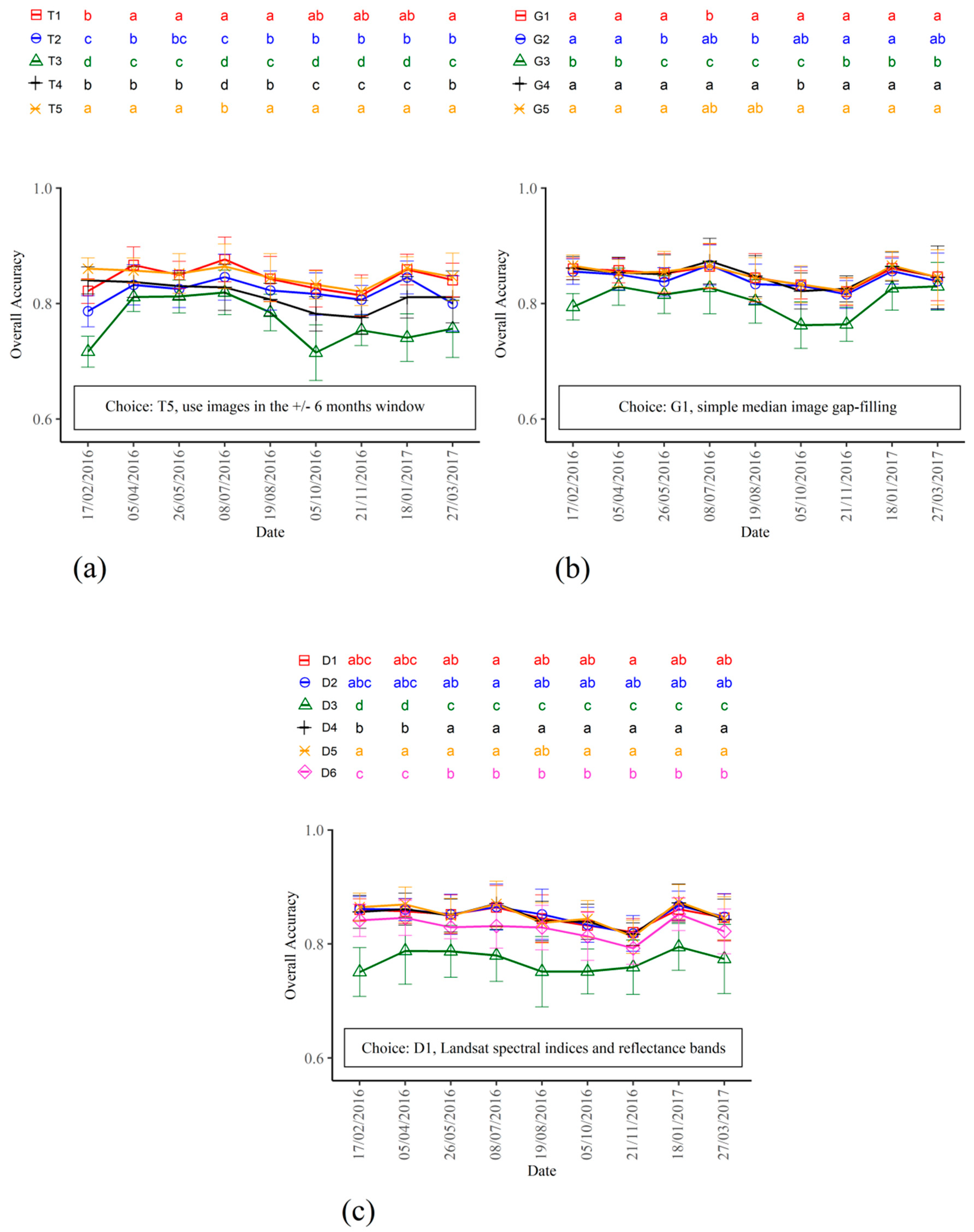
3.1. Selection of the Optimal Classification Options

The different options of the end-to-end classification method were chosen by iterative sequential tests. The optimal set of options, in terms of best OA for predicting independent data, was using 6 months of data before and 6 months after the predicted date (T5 in Table 3), a simple gap-filling with median values (G1), and only Landsat vegetation indices and spectral bands (D1). Figure 4 presents the comparison of the different options by changing the options one at a time, with the other options being fixed to the optimal ones.

Figure 4a shows that both options T5 (6 months before and 6 months after) and T1 (one year before) were not significantly different, except for two dates, with T5 being more accurate on 17/02/2016 and T1 the 08/07/2016. However, the advantage of using T5 was clearer in terms of OA for the first date, and T5 was, therefore, chosen as the optimal one. The other options for time-range yielded significantly lower results.

Figure 4b shows that the different gap-filling methods G1 and G4 were not significantly different except for two dates, G4 being more accurate on 08/07/2016 and G1 on 05/10/2016. G1 and G5 were not significantly different at all dates. Therefore, there was no clear improvement in using advanced gap-filling methods (linear interpolation or missForest algorithm) compared to using the band median value. G2 and G3 were options that discarded images having high gap proportion. When the threshold was strict (G3, 5%), the accuracy of the method declined because very few images were kept in the model (See Figure 3). With a threshold of 20% (G2), the result was statistically close to G1 at most dates, but not all.

Figure 4c shows few significant differences between the use of datasets D1, D2, D4, and D5. For the sake of simplicity, D1 was therefore chosen, since it contained a fewer number of predictors, only from Landsat. Sentinel-1 radar images alone (D3) or in conjunction with Landsat images (D4 and D5) did not significantly improve the results of D1. In this test, the RF algorithm was used, and a slight degradation of the results was obtained after dimensionality reduction (D6), probably because the importance threshold chosen to keep the predictor was too strict.

As a conclusion, the best set of options (i.e., T5-G1-D1) was selected, considering the McNemar comparison test as the first criterion, and when the options were not statistically different, the simplest one was considered. The same set of options were found for other levels of the nomenclature (not shown). It was clear that no unique set of options outweigh all others and that the best set of options differs between dates. For the sake of simplicity, the same final method with the simpler T5-G1-D1 options was applied for all dates and all classification levels.

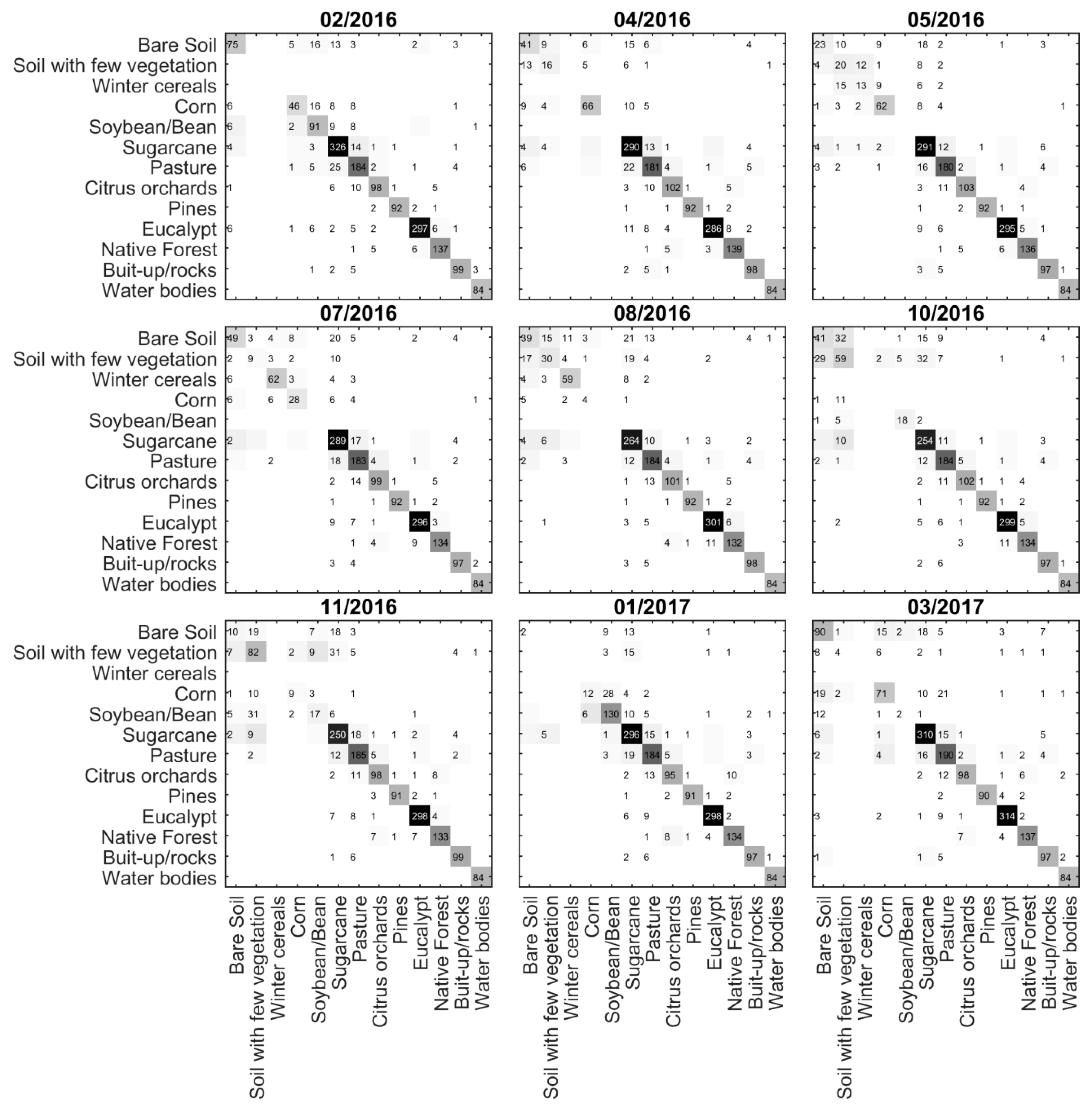
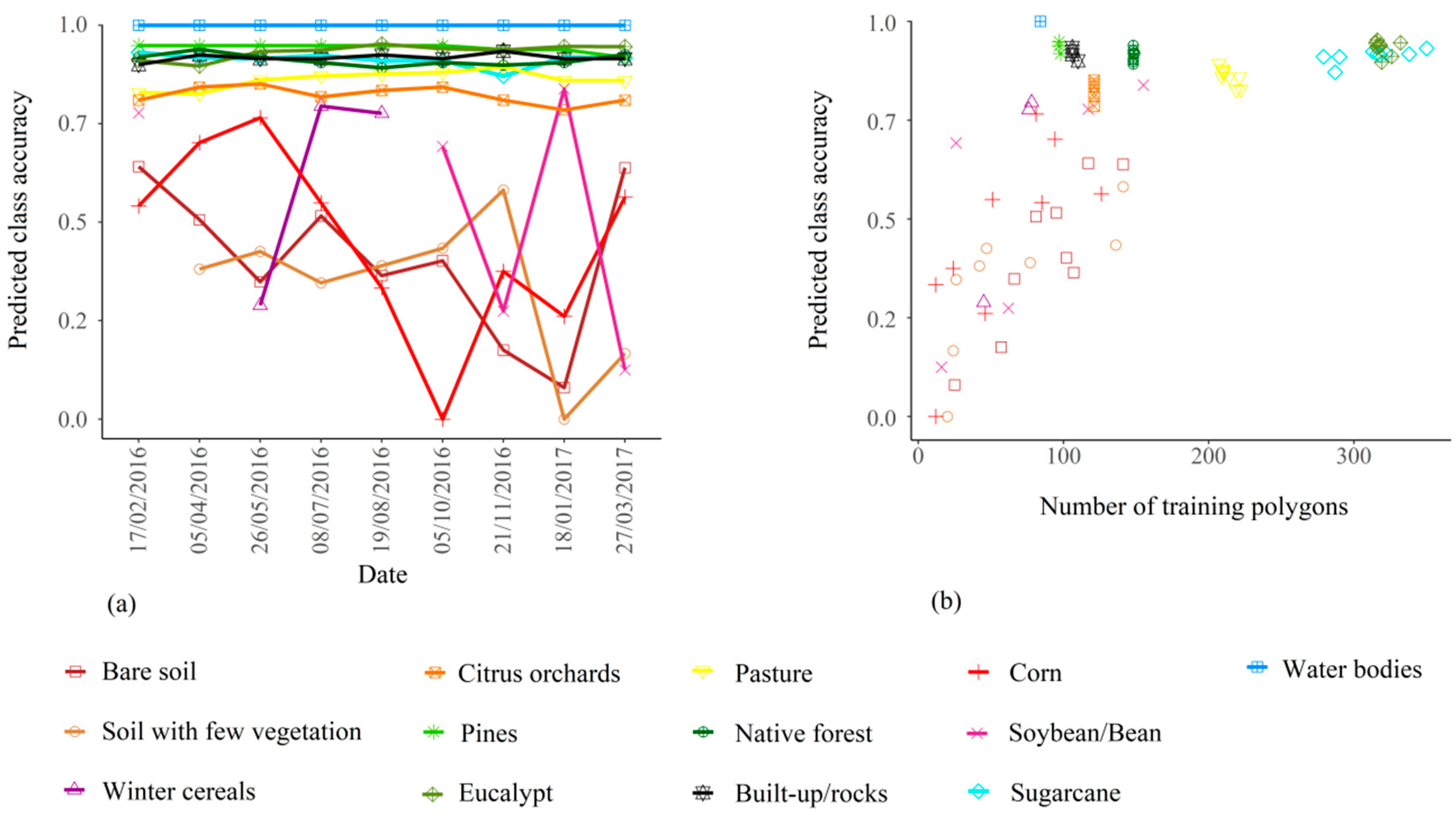
3.2. Confusion Matrices and Class Error Evolution

Figure 5 graphically represents the confusion matrices at each prediction date along the year, on independent polygons through CV. Interestingly, the pattern of the confusion matrices was persistent through time, even with a new calibration for each date. While the results were very good for the built-up, water bodies and most perennial vegetation classes, it was clear that the main remaining confusion originated from confusion between the bare soil, soil with few vegetation classes, and other annual crops. Indeed, these soil classes occurred for short periods at the beginning of all planted or sowed crops, with a variable crop calendar (Figure 2). Furthermore, the distinction between soils with few vegetation (including crop-emerging phase) and the grown crop was visually assessed in the field and, therefore, uncertain. Bare soil also had a large spectral variability, because it included soils that were plowed, with residues, sowed, and with different preceding vegetation classes such as annual crops, sugarcane, and even clear-cut forest plantations. Confusion was also present among the different classes of annual crops, when they are present at the same period. Finally, some confusion also existed between perennial classes, such as citrus orchards and natural vegetation.

The evolution of the prediction class accuracy (user accuracy) with time was computed based on the confusion matrices of Figure 5. Figure 6a shows that the classification accuracies were highly different among classes, with two types of evolution: either stable or high class accuracy through time, with values above 0.8 for permanent classes; or classes with lower accuracies that were variable with time for seasonally variable classes. There was a succession in the high accuracy values for the following classes: soybean in December–January, then summer corn from March to May, and then winter cereals from July to August. This finding corresponded to the known evolution of the crop cycles in the area under study, except for corn, which has a larger cultivation time spread and can be cultivated in winter. Bare soil and soil with few vegetation class accuracies depended also on the mapping date, with a peak in October.

The class accuracy was represented as a function of the number of polygons used in the training of the model for that class (Figure 6b) over the year. There was a clear positive association between the number of polygons and the predicted accuracy for most of the seasonal classes.

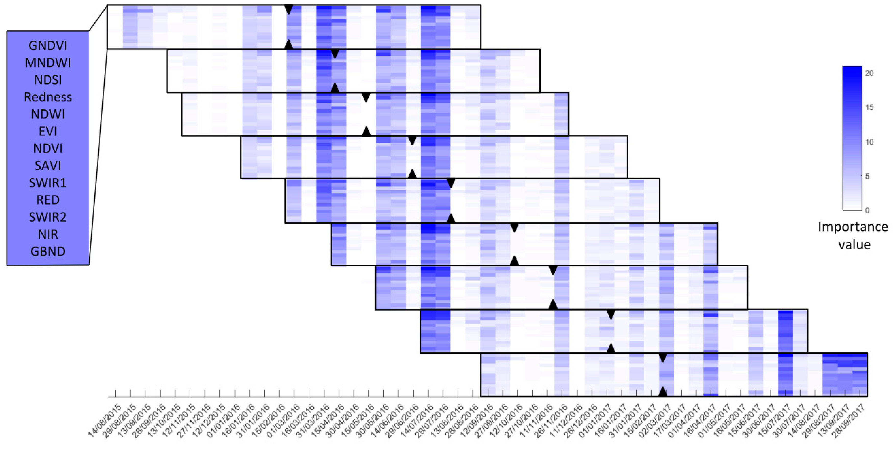
3.3. Predictor Importance as a Function of Landsat Image Date, Vegetation Indices and Predicted Date

To obtain more insight on the calibrated classifiers, the importance of the predictors over time was described in Figure 7. This figure represents the importance of the predictors in the final RF models. For a given classification date, ~25 images were used (T5 of Table 3), and 13 vegetation indices and spectral bands were used on each image. This approach yielded a total of ~325 importance values for each predicted date included in one black box in Figure 7. Some images were used as predictors for several prediction dates. Figure 7 shows that some images had clearly higher importance than others for a given prediction date. More interestingly, these important dates were the same across the different prediction dates. For instance, the composite images of 14 July to 28 July 2016 exhibited a high importance for all classifications performed between February 2016 and January 2017. On the other hand, some Landsat images were not important predictors, regardless of the prediction date and the vegetation index. Additionally, for a given prediction date, the important predictors were not coming only from a single Landsat image but from several and from different seasons. No correlation was found between the importance of a Landsat image and the prediction date, which indicated that the images that were the closest in time to the prediction date were not necessarily the most important.

Concerning the vegetation indices, the main trend was that the indices GNDVI and modified normalized difference water index (MNDWI) had higher importance than other indices, on all images. However, the indices NIR and Blue Green Normalized Difference (BGND) almost never exhibited a high importance. The ranking of indices changed slightly between Landsat images, but not much for a given Landsat image used for different prediction dates.

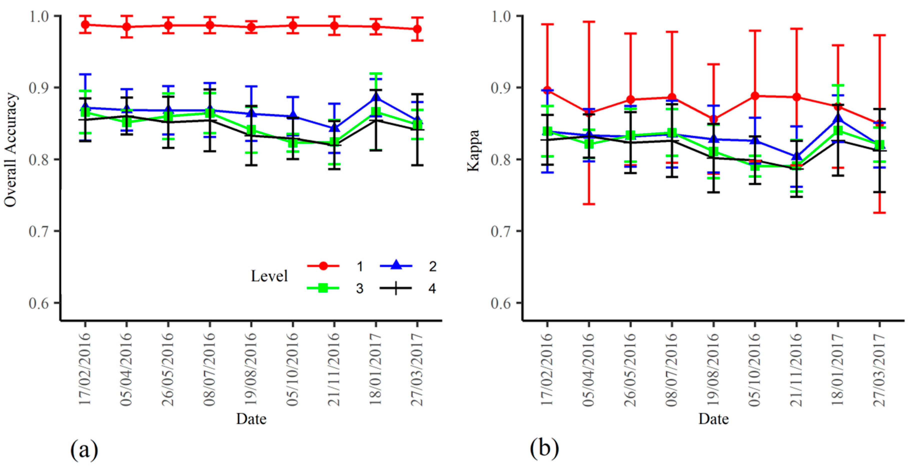
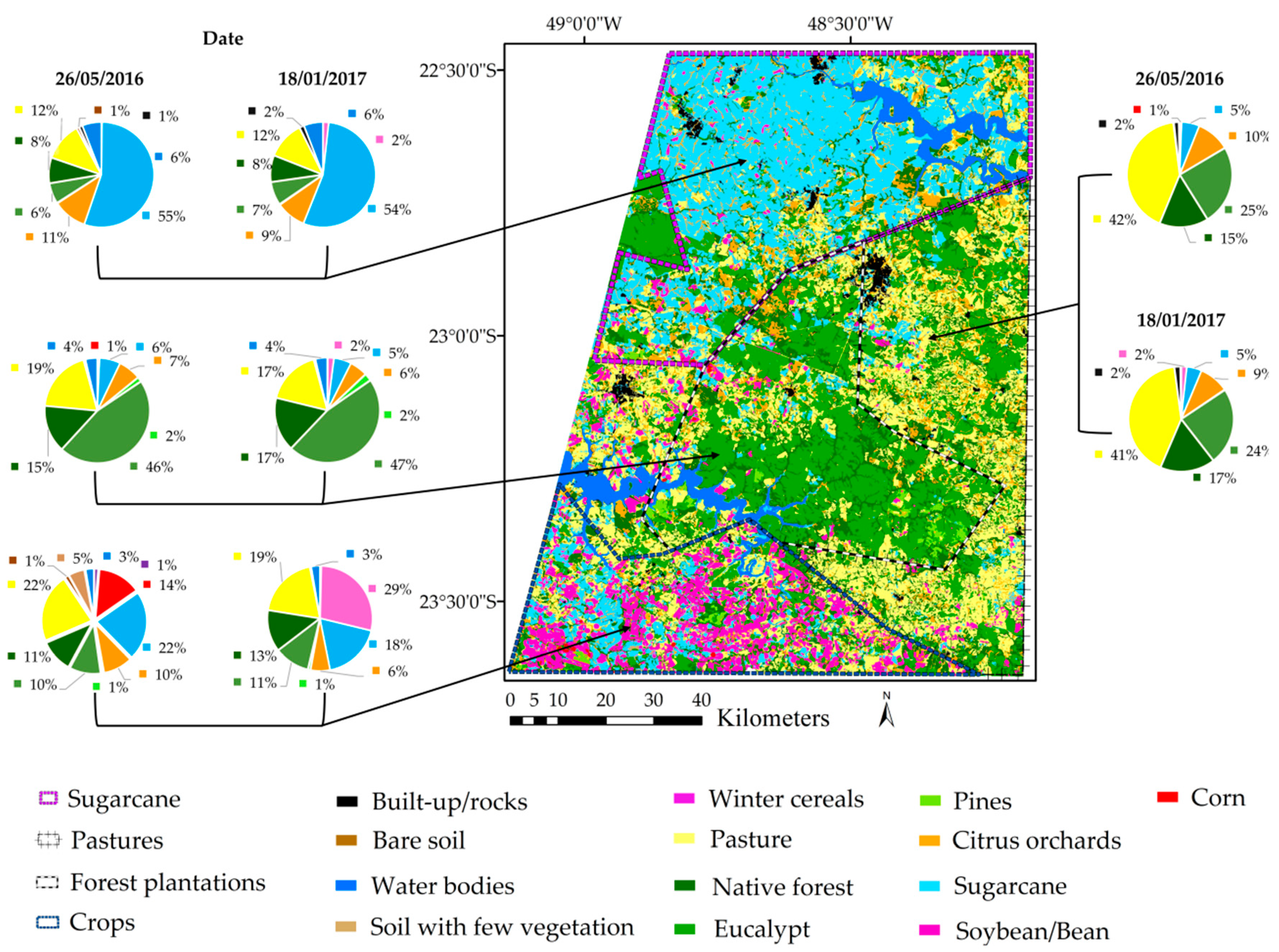
3.4. Classification Results

Figure 8 shows the estimation of the produced map accuracies based on the OA and the kappa statistics, as computed on CV of the observation dataset and corrected for class proportion. These values were high for the first level of the nomenclature, which corresponded to a vegetation/non-vegetation binary classification. For other classification levels (Level-2 to Level-4), the overall accuracy and kappa remained stable between 0.80 and 0.90, close to 0.85. The accuracy was only slightly higher for Level-2 than Level-3 and 4: sub-classifying the tree crops and the crops lowered the overall accuracy due to confusion among these classes. This finding indicated that the main classification errors of Level-3 and 4 were already present at Level-2.

The maps produced at the different levels showed high consistency, even if the algorithm was recalibrated each time. This region could be separated in 4 main areas (Figure 9), and the proportion of each land use was computed for May 2016 and January 2017 within each of these areas. As expected, major changes occurred in the crop area.

4. Discussion

The classification algorithm showed satisfactory results on the study site: corrected OA of 85% and K of 83% on average over the season for the more detailed classification levels. For the first level (vegetation/no vegetation), the classification accuracy was very high (OA of 99% and kappa of 90%). For the intermediary level 2, which differentiated pasture from annual crops from sugarcane, among others, the accuracy was intermediary (OA of 84%, kappa of 81%). These results fall into the range of precision obtained in other studies at similar level of classification including annual crop subclasses [84,85,86]. The present study site, however, is highly diverse, both as a result of the large size of the study area (12,000 km²) and the number of vegetation classes. Note that these accuracy metrics are based on roadside sampling and are therefore not probabilistic. Even if corrected for the class proportion, these values remain estimates of the real accuracies of the produced map, which could only be evaluated more precisely with extended probabilistic sampling over the entire area (e.g., random sampling without cross-validation), not feasible in this context. Surprisingly, the accuracy statistics (kappa or OA) were very stable along the season, in particular without any large drop during the cloudy season (see further discussion). The classification accuracy per class is presented in Figure 6, which indicates that high accuracies were reached for all perennial classes with average values higher than 0.8. The major errors came from annual crops, bare soils and soils with little vegetation, with a high confusion between these classes (Figure 5). However, the 3 major crops reached values >0.7 at some predicted dates. The discrimination between sugarcane, pasture and crops was high, with little confusion between these classes, while this was not obvious in other studies [62,87,88]. Similar methodologies that were used in the savannah landscape in Brazil also achieved good results for separating these classes [85,87]. Some confusion was observed on the final map between citrus orchards, which have distant trees with interlines covered with grass, and some types of natural forest with a low density of trees and grasses understory, or pastures with some trees (savannah-like) when visually comparing the classification with the SPOT high-resolution image. Such difficulties in class separation have been observed in other studies [86,89]. However, this is concerned with only a small part of the total area of the produced map, and a few percentages of these two classes. In addition, some classes with few frequencies in the dataset were discarded, which impacted the final produced map. Overall, the accuracy obtained with the 30 m resolution map on the 12,000 km² is high, which could be further enhanced with post-classification in future work (especially for perennial classes). These results indicate that the classifier could be applied at larger scale or could be recalibrated and applied in other regions; however, this generalization test should be properly undertaken [90].

The maps produced illustrate well the characteristics of the study sites in terms of highly diverse areas at the transition between the northern part of Sao Paulo state, cultivated mainly with sugarcane; the southern part of the area, which is the northern area of annual crops; the pastures in the West, which occupies a large part of Sao Paulo state; and forest plantations, which are generally located around pulp and paper industries [91]. This transitional area is interesting to test classification methods for further up-scaling. With such a map, it is possible to compare the proportion of certain types of land use as a function of dominant agricultural activities (e.g., natural forests in the 4 main areas). The method used satellite images before the prediction dates; it also showed good results (but slightly lower) upon using images from the previous year (T1 option, Figure 4a), allowing in-season crop monitoring.

An important aspect of the method was the definition of the classes, the hierarchical nomenclature and the predicted levels of classification. A new classifier was trained at each level (“Local Classifier Per Level Approach” defined in [92]); the advantage of this method was that for a given Level, all classes were classified, but it can create inconsistencies between levels. This was not a major issue here since the objective was to analyze how the aggregation of classes between the four levels may influence the classification results. A crop/non-crop classification was previously performed in the same area in a previous study [14] with good accuracy, but it underlined the difficulty to adopt such division, particularly when annual crops are mixed with perennial crops such as sugarcane and cultivated pastures. Based on these results, a choice was made here to distinguish from Level 2 the sugarcane plantations from annual crops and the ligneous plantations from natural vegetation and pastures. Since the study was dedicated to in-season classification, it was decided to have a separate bare soil and soil with few green vegetation classes. They were mainly present in the transitional phases in cropping systems, planted pastures, and forest plantation clear-cuts, as performed in other within-season crop mapping. There is no consensus whether or not this class should be distinguished from the previous or following crop. Studies dealing with within-season classification may include such a class, i.e., the crop is classified only when it has a sufficient vegetation development (e.g., [61]). Others do not separate the growing stages and consider, for instance, a bare soil-corn-bare soil succession as the “corn” class, and only fields with bare soil throughout the year are considered as “bare soil” classes (e.g., [93]). In-season classification tries to produce a map of the land use at a time t, including eventual transitional phases. Post-classification that analyzes the land-use succession along the year can be used later to distinguish the crop succession.

Different methods listed in Table 3 were tested before obtaining the results described above. Many other options were not tested, when we found a higher consensus in the literature, for instance, for the use of object-based classification instead of pixel-based classification (e.g., [94]) or the use of the random forest classifier (e.g., review by [73]). Calibration of segmentation parameters can be included in the classification process [95]. This procedure was performed in a previous study [25] for classifying sugarcane areas in the same region and with similar Landsat data, but no large improvements were expected by changing these segmentation parameters. However, using a higher-resolution image to create the polygon objects could have improved the definition of the boundaries (e.g., roads and field limits).

The use of Sentinel-1 SAR data did not improve the classification results, in contrast to many studies reported in the literature. Sentinel-1 time series alone only reached accuracies of 77% on an average for classification when VV, VH and their ratio and sum were used. The low information on VV and VH signals of SAR C-band for agricultural classification was already observed when used alone on a single date, while using time-series of SAR improved the classification [41]. The SAR data did not help with discriminating classes not already well separated with optical images only in our study, even when using all available images. Backscatter intensities are influenced by many surface properties such as the size of the plant and the proportion of stem, branches, foliage, soil, and their humidity and dieletric properties, as well as acquisition characteristics, such as frequency, polarization and incidence angles [96,97]. A previous study [98] used SAR–C band measurements in barley, oat, canola and wheat to show the importance of incidence angle, with better discrimination and higher incidence angle. In addition, the polarization can influence the discrimination, e.g., the authors found that the HV backscatter improved the discrimination between canola and soybean and that VV and HH backscatters are similar in case of high biomass. Other approaches, such as texture, polarization ratio, quad-pol or dual polarization and decomposition, can improve the discrimination [31,98,99]. Even if our first simple use of Sentinel-1 data was not successful in this context, more detailed work should be performed on Sentinel-1 data considering the aspects discussed above, such as filtering for noise and incidence angle and performing textural analysis.

The use of Landsat textural information, presented in this study as simple polygon-scale standard deviations of NDVI and GNDVI only, did not significantly improve the OA. Therefore, we emphasize that future development would be needed to enhance the use of this type of textural predictors, which have been demonstrated to be efficient in other contexts [100], by finding adapted co-occurrence statistics, for instance, or using images with higher spatial resolution. This approach would probably require the use of higher-resolution images. These results showed that the main information for the classification was obtained from the optical reflectance indices and spectral bands averaged at the polygon scale. The best indices (sorted with the random forest importance metrics) were GNDVI and MNDWI. GNDVI, a normalized difference between green and near-infrared, was already determined to be an important discriminating feature in a previous study [49] (same index with the name “NDWI” in their study). Next, vegetation indices using the SWIR1 were the most important, which was also found to be useful for crop identification in other studies [25,61]. The use of single band reflectance (NIR, RED and SWIR2) and visible-only index GBND appeared as weak predictors compared to other indices.

The most important information for classifying the agricultural landscape under study was the temporal information obtained from the use of a series of images. Reducing the time window to three months before the prediction date or 3 months before and 3 months later reduced the OA from 0.85 to 0.76 (Figure 4a). On the other hand, a one-year long window significantly increased the overall accuracy. This was also observed in other studies on agricultural mapping [39,84,87]. The results of the present study show that the importance of the predictors is clearly a function of the image acquisition date, more than a question of spectral index type. Interestingly, the most important image predictors were not a function of the calibration and prediction date but were mostly associated with the image quality itself. The important dates were common for different prediction dates. For instance, all indices and band reflectance computed from the composite image of the first 15 days of July 2016 were highly important for all prediction dates of the season. This finding was due to several reasons: (i) a large proportion of observations were for permanent crops and did not change within a year. Thus, the image which discriminated the best of these land covers was more important. The image in July (winter dry season), allowed such discrimination between these vegetation types; (ii) the quality of the image played an important role, since gap-filling of a large part of an image will result in higher uncertainty; (iii) even for annual crops, the land use in winter brought indirect information on the land use in summer due to time-correlation in the observation set. However, even if some precise Landsat images were very important, other images at other dates were also necessary. Attempts to reduce the independent variables only resulted in significant loss of accuracy.

As a consequence, using time series had the primary advantage of including some important images in the season mostly for perennial classes, and supplementary images for crop classification. However, this second aspect showed some limitation since the confusion remained high among the crop classes. The fine changes detected during field measurements, especially the transition phases during crop succession, could not be solved with the good quality Landsat image frequency, even if image compositing and gap-filling was used.

The percentage of clouds during summer was high in the region. Our results showed that the soybean summer crop was classified with a reasonable OA between 0.5 and 0.8, resulting from the gap-filling methodologies. Our results underlined the fact that the gap-filling step of the image was critical. Indeed, a simple removal of the image composites when they had more than 5% of gaps (clouds, cloud shadow or images issues) decreased the overall accuracy. Keeping only the images having between 0 and 20% of gaps and gap-filling allowed us to reach almost the same accuracy as using all gap filled image. In other words, there was significant information used in the classification of these images, with the percentage of gaps between 0 and 20%. The different gap-filling methods utilized here provided equivalent results. Future improvements in the method could include a different gap-filling methodology, either using the fusion approach with more frequent images, such as MODIS, or directly using images from satellites with more frequent revisit times, such as Sentinel-2, which allows the use of more composite images without gaps.

For the major land use of the study area, the classification gave a low class error: forests, forest plantations, sugarcane, and pastures showed accuracies above 0.85. Annual crop classes remained the most difficult to classify and these, therefore, require more attention. An interesting result is that the crop class-accuracy exhibited an error proportional to the number of observations used during training. This could be a direct effect of the algorithm, which showed a better ability to identify the intra-class variability. This effect was still observable for sugarcane even with a large number of observations but not for other classes such as water bodies or Eucalyptus plantations. The high temporal sampling of field in the season allowed to characterize the period when the crop class accuracies were the highest. These periods corresponded to the window where one crop was more spectrally different from the other, which may not be exactly at the peak growth; however, it was linked to the period when more observations were collected for that class. This underlines the fact that it is not sufficient to select the observation date only based on the vegetation peak stage of the crop. For instance, the class accuracy was high for soybean in December–January, while that for summer corn was detected from March to May and that for winter cereals was identified from July to August, even though their growing periods were longer than these periods (Figure 2). A recommendation would be to dedicate the field-sampling efforts during these periods, thereby increasing the number of field observations.

5. Conclusions

This study presents a reliable classification method for a highly diverse subtropical landscape at a sub-regional scale (12,000 km²). The study area is roughly divided into 4 agricultural regions with a majority of pastures, forest plantations, sugarcane and annual crops, and a unique classifier was applied across all the regions. The overall accuracy was high at the more detailed level (0.84). Many classes that are highly represented in the region, mostly perennials, were well-classified. The annual crop class exhibited medium accuracies most of the time, mostly due to confusion with the two soil classes (bare soil and soil with few vegetation) and confusion with other concomitant crops. Finally, the best method was also one of the simplest: composite images of Landsat indices and single band reflectance, extracted within a 1-year time-window around the prediction date, averaged by polygons after segmentation, with a simple cloud and cloud shadow gap-filling.

The major findings are that (1) the use of image time series in the applied method is essential to obtain highly discriminant images that are eventually distant in time, which are images with the lowest cloud-cover. Additional images of lower quality improve the sub-class and dynamic class separation. (2) These highly discriminant images are important for classification at different dates over the season. (3) A simple gap-filling method is sufficient compared to linear interpolations or higher complexity algorithms such as MissForest. (4) Spectral indices including red, NIR, and SWIR bands are the most important in the calibrated model, while Sentinel-1 and simple textural indices computed from Landsat data do not significantly improve the results. (5) The classification along the season also shows that there are three periods of field measurements in that region, which are useful for classifying the main crops during the year and are not necessary at the class vegetation peak, and that the number of field observations should be concentrated at these periods.

References

1. Foley, J.A.; Ramankutty, N.; Brauman, K.A.; Cassidy, E.S.; Gerber, J.S.; Johnston, M.; Mueller, N.D.; O’Connell, C.; Ray, D.K.; West, P.C.; et al. Solutions for a cultivated planet. Nature 2011, 478, 337–342. [Google Scholar] [CrossRef] [PubMed]
2. Pelletier, N.; Tyedmers, P. Forecasting potential global environmental costs of livestock production 2000–2050. PNAS 2010, 107, 18371–18374. [Google Scholar] [CrossRef]
3. IAASTD—International Assessment of Agricultural Knowledge, Science, and Technology for Development. Agriculture at a Crossroads—Global Report; McIntype, B.D., Herren, H.R., Wakhungu, J., Watson, R.T., Eds.; Island Press: Washington, DC, USA, 2009; Volume 320, ISBN 978-1-59726-538-6. [Google Scholar]
4. Gao, F.; Wang, Q.; Dong, J.; Xu, Q. Spectral and spatial classification of hyperspectral images based on random multi-graphs. Remote Sens. 2018, 10, 1271. [Google Scholar] [CrossRef]
5. Torbick, N.; Huang, X.; Ziniti, B.; Johnson, D.; Masek, J.; Reba, M. Fusion of moderate resolution earth observations for operational crop type mapping. Remote Sens. 2018, 10, 1058. [Google Scholar] [CrossRef]
6. Kolotii, A.; Kussul, N.; Shelestov, A.; Skakun, S.; Yailymov, B.; Basarab, R.; Lavreniuk, M.; Oliinyk, T.; Ostapenko, V. Comparison of biophysical and satellite predictors for wheat yield forecasting in Ukraine. Int. Arch. Photogramm. Remote Sens. Spat. Inf. Sci. ISPRS Arch. 2015, 40, 39–44. [Google Scholar] [CrossRef]
7. Whitcraft, A.K.; Vermote, E.F.; Becker-Reshef, I.; Justice, C.O. Cloud cover throughout the agricultural growing season—Impacts on passive optical earth observations. Remote Sens. Environ. 2015, 156, 438–447. [Google Scholar] [CrossRef]
8. Fritz, S.; See, L.; Mccallum, I.; You, L.; Bun, A.; Moltchanova, E.; Duerauer, M.; Albrecht, F.; Schill, C.; Perger, C.; et al. Mapping global cropland and field size. Glob. Chang. Biol. 2015, 21, 1980–1992. [Google Scholar] [CrossRef] [PubMed]
9. Formaggio, A.R.; Sanches, I.D. Sensoriamento Remoto em Agricultura, 1st ed.; Oficina de Textos: São Paulo, Brazil, 2017; ISBN 978-85-7975-277-3. [Google Scholar]
10. FAO—Food and Agriculture Organization of the United Nations. FAOSTAT Statistical Database 2015; FAO: Rome, Italy, 2015. [Google Scholar]
11. Del’Arco Sanches, I.; Feitosa, R.Q.; Achanccaray Diaz, P.M.; Dias Soares, M.; Barreto Luiz, A.J.; Schultz, B.; Pinheiro Maurano, L.E. Campo Verde database: Seeking to improve agricultural remote sensing of tropical areas. IEEE Geosci. Remote Sens. Lett. 2018, 15, 369–373. [Google Scholar] [CrossRef]
12. IBGE—Instituto Brasileiro de Geografia e Estatística- Censo Agropecuário 2017- Produção Agrícola Municipal. Available online: https://sidra.ibge.gov.br/pesquisa/pam/tabelas (accessed on 25 October 2018).
13. Gallego, F.J.; Kussul, N.; Skakun, S.; Kravchenko, O.; Shelestov, A.; Kussul, O. Efficiency assessment of using satellite data for crop area estimation in Ukraine. Int. J. Appl. Earth Obs. Geoinf. 2014, 29, 22–30. [Google Scholar] [CrossRef]
14. Waldner, F.; De Abelleyra, D.; Verón, S.R.; Zhang, M.; Wu, B.; Plotnikov, D.; Bartalev, S.; Lavreniuk, M.; Skakun, S.; Kussul, N.; et al. Towards a set of agrosystem-specific cropland mapping methods to address the global cropland diversity. Int. J. Remote Sens. 2016, 37, 3196–3231. [Google Scholar] [CrossRef]
15. Azzari, G.; Jain, M.; Lobell, D.B. Towards fine resolution global maps of crop yields: Testing multiple methods and satellites in three countries. Remote Sens. Environ. 2017, 202, 129–141. [Google Scholar] [CrossRef]
16. Xiong, J.; Thenkabail, P.S.; Gumma, M.K.; Teluguntla, P.; Poehnelt, J.; Congalton, R.G.; Yadav, K.; Thau, D. Automated cropland mapping of continental Africa using Google Earth Engine cloud computing. ISPRS J. Photogramm. Remote Sens. 2017, 126, 225–244. [Google Scholar] [CrossRef]
17. Kussul, N.; Lavreniuk, M.; Skakun, S.; Shelestov, A. Deep learning classification of land cover and crop types using remote sensing data. IEEE Geosci. Remote Sens. Lett. 2017, 14, 778–782. [Google Scholar] [CrossRef]
18. Le Maire, G.; Dupuy, S.; Nouvellon, Y.; Loos, R.A.; Hakamada, R. Mapping short-rotation plantations at regional scale using MODIS time series: Case of eucalypt plantations in Brazil. Remote Sens. Environ. 2014, 152, 136–149. [Google Scholar] [CrossRef]
19. Matton, N.; Canto, G.S.; Waldner, F.; Valero, S.; Morin, D.; Inglada, J.; Arias, M.; Bontemps, S.; Koetz, B.; Defourny, P. An automated method for annual cropland mapping along the season for various globally-distributed agrosystems using high spatial and temporal resolution time series. Remote Sens. 2015, 7, 13208–13232. [Google Scholar] [CrossRef]
20. Lebourgeois, V.; Dupuy, S.; Vintrou, É.; Ameline, M.; Butler, S.; Bégué, A. A combined random forest and OBIA classification scheme for mapping smallholder agriculture at different nomenclature levels using multisource data (simulated Sentinel-2 time series, VHRS and DEM). Remote Sens. 2017, 9, 259. [Google Scholar] [CrossRef]
21. Hay, G.J.; Castilla, G. Geographic Object- Based Image Analysis (GEOBIA): A new name for a new discipline. In Object-Based Image Analysis- Spatial Concepts for Knowledge- Driven Remote Sensing Applications; Blaschke, T., Lang, S., Hay, G.J., Eds.; Springer: Berlin, Germany, 2008; pp. 77–89. ISBN 978-3-540-77057-2. [Google Scholar]
22. Costa, H.; Carrão, H.; Bação, F.; Caetano, M. Combining per-pixel and object-based classifications for mapping land cover over large areas. Int. J. Remote Sens. 2014, 35, 738–753. [Google Scholar] [CrossRef]
23. Blaschke, T. Object based image analysis for remote sensing. ISPRS J. Photogramm. Remote Sens. 2010, 65, 2–16. [Google Scholar] [CrossRef]
24. Ma, L.; Li, M.; Ma, X.; Cheng, L.; Du, P.; Liu, Y. A review of supervised object-based land-cover image classification. ISPRS J. Photogramm. Remote Sens. 2017, 130, 277–293. [Google Scholar] [CrossRef]
25. Dos Santos Luciano, A.C.; Picoli, M.C.A.; Rocha, J.V.; Franco, H.; Junqueira, C.; Sanches, G.M. Generalized space-time classifiers for monitoring sugarcane areas in Brazil. Remote Sens. Environ. 2018, 215, 438–451. [Google Scholar] [CrossRef]
26. Khatami, R.; Mountrakis, G.; Stehman, S.V. A meta-analysis of remote sensing research on supervised pixel-based land-cover image classification processes: General guidelines for practitioners and future research. Remote Sens. Environ. 2016, 177, 89–100. [Google Scholar] [CrossRef]
27. Huang, Y.; Jiang, D.; Zhuang, D. Filling gaps in vegetation index measurements for crop growth monitoring. Afr. J. Agric. Res. 2011, 6, 2920–2930. [Google Scholar] [CrossRef]
28. Whitcraft, A.K.; Becker-Reshef, I.; Justice, C.O. A framework for defining spatially explicit earth observation requirements for a global agricultural monitoring initiative (GEOGLAM). Remote Sens. 2015, 7, 1461–1481. [Google Scholar] [CrossRef]
29. Dara, A.; Baumann, M.; Kuemmerle, T.; Pflugmacher, D.; Rabe, A.; Griffiths, P.; Hölzel, N.; Kamp, J.; Freitag, M.; Hostert, P. Mapping the timing of cropland abandonment and recultivation in northern Kazakhstan using annual Landsat time series. Remote Sens. Environ. 2018, 213, 49–60. [Google Scholar] [CrossRef]
30. Tatsumi, K.; Yamashiki, Y.; Canales Torres, M.A.; Taipe, C.L.R. Crop classification of upland fields using Random forest of time-series Landsat 7 ETM+ data. Comput. Electron. Agric. 2015, 115, 171–179. [Google Scholar] [CrossRef]
31. Inglada, J.; Vincent, A.; Arias, M.; Marais-Sicre, C. Improved early crop type identification by joint use of high temporal resolution sar and optical image time series. Remote Sens. 2016, 8, 362. [Google Scholar] [CrossRef]
32. Zhu, Z.; Woodcock, C.E.; Holden, C.; Yang, Z. Generating synthetic Landsat images based on all available Landsat data: Predicting Landsat surface reflectance at any given time. Remote Sens. Environ. 2015, 162, 67–83. [Google Scholar] [CrossRef]
33. Eberhardt, I.D.R.; Schultz, B.; Rizzi, R.; Sanches, I.D.A.; Formaggio, A.R.; Atzberger, C.; Mello, M.P.; Immitzer, M.; Trabaquini, K.; Foschiera, W.; et al. Cloud cover assessment for operational crop monitoring systems in tropical areas. Remote Sens. 2016, 8, 219. [Google Scholar] [CrossRef]
34. Roy, D.P.; Ju, J.; Lewis, P.; Schaaf, C.; Gao, F.; Hansen, M.; Lindquist, E. Multi-temporal MODIS–Landsat data fusion for relative radiometric normalization, gap filling, and prediction of Landsat data. Remote Sens. Environ. 2008, 112, 3112–3130. [Google Scholar] [CrossRef]
35. Gao, F.; Masek, J.; Schwaller, M.; Hall, F. On the blending of the landsat and MODIS surface reflectance: Predicting daily landsat surface reflectance. IEEE Trans. Geosci. Remote Sens. 2006, 44, 2207–2218. [Google Scholar] [CrossRef]
36. Skakun, S.V.; Basarab, R.M. Reconstruction of missing data in time-series of optical satellite images using self-organizing Kohonen maps. J. Autom. Inf. Sci. 2014, 46, 19–26. [Google Scholar] [CrossRef]
37. Ndikumana, E.; Ho, D.; Minh, T.; Baghdadi, N.; Courault, D.; Hossard, L. Deep recurrent neural network for agricultural classification using multitemporal SAR Sentinel-1 for Camargue, France. Remote Sens. 2018, 10, 1217. [Google Scholar] [CrossRef]
38. Jia, K.; Liang, S.; Zhang, N.; Wei, X.; Gu, X.; Zhao, X.; Yao, Y.; Xie, X. Land cover classification of finer resolution remote sensing data integrating temporal features from time series coarser resolution data. ISPRS J. Photogramm. Remote Sens. 2014, 93, 49–55. [Google Scholar] [CrossRef]
39. Kussul, N.; Lemoine, G.; Gallego, F.J.; Skakun, S.V.; Lavreniuk, M.; Shelestov, A.Y. Parcel-based crop classification in ukraine using Landsat-8 data and Sentinel-1A data. IEEE J. Sel. Top. Appl. Earth Obs. Remote Sens. 2016, 9, 2500–2508. [Google Scholar] [CrossRef]
40. Inoue, Y.; Kurosu, T.; Maeno, H.; Uratsuka, S.; Kozu, T.; Dabrowska-Zielinska, K.; Qi, J. Season long daily measurements of multifrequency (Ka, Ku, X, C, and L) and full polarization backscatter signatures over paddy rice field and their relationship with biological variables_20.pdf. Remote Sens. Environ. 2002, 81, 194–204. [Google Scholar] [CrossRef]
41. Skriver, H.; Mattia, F.; Satalino, G.; Balenzano, A.; Pauwels, V.R.N.; Verhoest, N.E.C.; Davidson, M. Crop classification using short-revisit multitemporal SAR data. IEEE J. Sel. Top. Appl. Earth Obs. Remote Sens. 2011, 4, 423–431. [Google Scholar] [CrossRef]
42. Hütt, C.; Waldhoff, G. Multi-data approach for crop classification using multitemporal, dual-polarimetric TerraSAR-X data, and official geodata. Eur. J. Remote Sens. 2017, 51, 62–74. [Google Scholar] [CrossRef]
43. Li, C.; Wang, J.; Wang, L.; Hu, L.; Gong, P. Comparison of classification algorithms and training sample sizes in urban land classification with landsat thematic mapper imagery. Remote Sens. 2014, 6, 964–983. [Google Scholar] [CrossRef]
44. Berhane, T.; Lane, C.; Wu, Q.; Autrey, B.; Anenkhonov, O.; Chepinoga, V.; Liu, H. Decision-tree, rule-based, and random forest classification of high-resolution multispectral imagery for wetland mapping and inventory. Remote Sens. 2018, 10, 580. [Google Scholar] [CrossRef] [PubMed]
45. Chen, Y.; Lu, D.; Moran, E.; Batistella, M.; Dutra, L.V.; Sanches, I.D.; Da Silva, R.F.B.; Huang, J.; Luiz, A.J.B.; De Oliveira, M.A.F. Mapping croplands, cropping patterns, and crop types using MODIS time-series data. Int. J. Appl. Earth Obs. Geoinf. 2018, 69, 133–147. [Google Scholar] [CrossRef]
46. Knorn, J.; Rabe, A.; Radeloff, V.C.; Kuemmerle, T.; Kozak, J.; Hostert, P. Land cover mapping of large areas using chain classification of neighboring Landsat satellite images. Remote Sens. Environ. 2009, 113, 957–964. [Google Scholar] [CrossRef]
47. Melgani, F.; Bruzzone, L. Classification of hyperspectral remote sensing images with support vector machines. IEEE Trans. Geosci. Remote Sens. 2004, 42, 1778–1790. [Google Scholar] [CrossRef]
48. Shi, D.; Yang, X. Support vector machines for land cover mapping from remote sensor imagery. In Monitoring and Modeling of Global Changes: A Geomatics Perspective; Li, J., Yang, X., Eds.; Springer: New York, NY, USA, 2015; pp. 265–279. ISBN 978-94-017-9812-9. [Google Scholar]
49. Inglada, J.; Arias, M.; Tardy, B.; Hagolle, O.; Valero, S.; Morin, D.; Dedieu, G.; Sepulcre, G.; Bontemps, S.; Defourny, P.; et al. Assessment of an operational system for crop type map production using high temporal and spatial resolution satellite optical imagery. Remote Sens. 2015, 7, 12356–12379. [Google Scholar] [CrossRef]
50. Noi, P.T.; Kappas, M. Comparison of random forest, k-nearest neighbor, and support vector machine classifiers for land cover classification using sentinel-2 imagery. Sensors 2018, 18, 18. [Google Scholar] [CrossRef]
51. De Souza Rolim, G.; Lucas, L.E. Camargo, Köppen and Thornthwaite climate classification systems in defining climatical regions of the state of São Paulo, Brazil. Int. J. Climatol. 2016, 36, 636–643. [Google Scholar] [CrossRef]
52. Camargo, A.D. Classificação Climática para Zoneamento de Aptidão Agroclimática. 1991. Available online: https://scholar.google.co.uk/scholar?hl=en&as_sdt=0%2C5&q=+Classifica%C3%A7%C3%A3o+clim%C3%A1tica+para+zoneamento+de+aptid%C3%A3o+agroclim%C3%A1tica&btnG= (accessed on 8 February 2019).
53. Maluf, J.R.T. Nova classificação climática do Estado do Rio Grande do Sul. A new climatic classification for the State of Rio Grande do Sul, Brazil. Rev. Bras. Agrometeorol. 2000, 8, 141–150. [Google Scholar]
54. Gorelick, N.; Hancher, M.; Dixon, M.; Ilyushchenko, S.; Thau, D.; Moore, R. Google Earth Engine: Planetary-scale geospatial analysis for everyone. Remote Sens. Environ. 2017, 202, 18–27. [Google Scholar] [CrossRef]
55. Masek, J.G.; Vermote, E.F.; Saleous, N.E.; Wolfe, R.; Hall, F.G.; Huemmrich, K.F.; Gao, F.; Kutler, J.; Lim, T. A Landsat surface reflectance dataset. IEEE Geosci. Remote Sens. Lett. 2006, 3, 68–72. [Google Scholar] [CrossRef]
56. Schmidt, G.; Jenkerson, C.; Masek, J.; Vermote, E.; Gao, F. Landsat ecosystem disturbance adaptive processing system (LEDAPS) algorithm description. Open File Rep. 2013–1057 2013, 1–27. [Google Scholar] [CrossRef]
57. Foga, S.; Scaramuzza, P.L.; Guo, S.; Zhu, Z.; Dilley, R.D.; Beckmann, T.; Schmidt, G.L.; Dwyer, J.L.; Joseph Hughes, M.; Laue, B. Cloud detection algorithm comparison and validation for operational Landsat data products. Remote Sens. Environ. 2017, 194, 379–390. [Google Scholar] [CrossRef]
58. Diek, S.; Fornallaz, F.; Schaepman, M.E.; De Jong, R. Barest pixel composite for agricultural areas using landsat time series. Remote Sens. 2017, 9, 1245. [Google Scholar] [CrossRef]
59. Belgiu, M.; Csillik, O. Sentinel-2 cropland mapping using pixel-based and object-based time-weighted dynamic time warping analysis. Remote Sens. Environ. 2018, 204, 509–523. [Google Scholar] [CrossRef]
60. Vieira, M.A.; Formaggio, A.R.; Rennó, C.D.; Atzberger, C.; Aguiar, D.A.; Mello, M.P. Object based image analysis and data mining applied to a remotely sensed Landsat time-series to map sugarcane over large areas. Remote Sens. Environ. 2012, 123, 553–562. [Google Scholar] [CrossRef]
61. Peña-barragán, J.M.; Ngugi, M.K.; Plant, R.E.; Six, J. Object-based crop identification using multiple vegetation indices, textural features and crop phenology. Remote Sens. Environ. 2011, 115, 1301–1316. [Google Scholar] [CrossRef]
62. Xavier, A.C.; Rudorff, B.F.T.; Shimabukuro, Y.E.; Berka, L.M.S.; Moreira, M.A. Multi-temporal analysis of MODIS data to classify sugarcane crop. Int. J. Remote Sens. 2006, 27, 755–768. [Google Scholar] [CrossRef]
63. Rouse, J.W.; Hass, R.H.; Schell, J.A.; Deering, D.W. Monitoring vegetation systems in the great plains with ERTS. Third ERTS Symp. NASA 1973, 1, 309–317. [Google Scholar]
64. Huete, A.R.; Liu, H.; van Leeuwen, W.J. The use of vegetation indices in forested regions: issues of linearity and saturation. In Geoscience and Remote Sensing, 1997. IGARSS’97. Remote Sensing-A Scientific Vision for Sustainable Development, 1997 IEEE International; IEEE: Singapore, 1997; Volume 4, pp. 1966–1968. [Google Scholar] [CrossRef]
65. Huete, A.R. A soil-adjusted vegetation index (SAVI). Remote Sens. Environ. 1988, 25, 295–309. [Google Scholar] [CrossRef]
66. Gao, B.C. NDWI—A normalized difference water index for remote sensing of vegetation liquid water from space. Remote Sens. Environ. 1996, 58, 257–266. [Google Scholar] [CrossRef]
67. Gitelson, A.A.; Kaufman, Y.J.; Merzlyak, M.N. Use of a green channel in remote sensing of global vegetation from EOS-MODIS. Remote Sens. Environ. 1996, 58, 289–298. [Google Scholar] [CrossRef]
68. Hall, D.K.; Riggs, G.A.; Salomonson, V.V. Development of methods for mapping global snow cover using moderate resolution imaging spectroradiometer data. Remote Sens. Environ. 1995, 54, 127–140. [Google Scholar] [CrossRef]
69. Xu, H. Modification of normalised difference water index (NDWI) to enhance open water features in remotely sensed imagery. Int. J. Remote Sens. 2006, 27, 3025–3033. [Google Scholar] [CrossRef]
70. Madeira, J.; Bedidi, A.; Cervelle, B.; Pouget, M.; Flay, N. Visible spectrometric indices of hematite (Hm) and goethite (Gt) content in lateritic soils: The application of a Thematic Mapper (TM) image for soil-mapping in Brasilia, Brazil. Int. J. Remote Sens. 1997, 18, 2835–2852. [Google Scholar] [CrossRef]
71. Stekhoven, D.J.; Bühlmann, P. Missforest-non-parametric missing value imputation for mixed-type data. Bioinformatics 2012, 28, 112–118. [Google Scholar] [CrossRef] [PubMed]
72. Breiman, L. Random forests. Mach. Learn. 2001, 45, 5–32. [Google Scholar] [CrossRef]
73. Belgiu, M.; Drăgu, L. Random forest in remote sensing: A review of applications and future directions. ISPRS J. Photogramm. Remote Sens. 2016, 114, 24–31. [Google Scholar] [CrossRef]
74. Wright, M.N.; Ziegler, A. Ranger: A fast implementation of random forests for high dimensional data in C++ and R. J. Stat. Softw. 2017, 77, 1–17. [Google Scholar] [CrossRef]
75. Waldner, F.; Bellemans, N.; Hochman, Z.; Newby, T.; De Abelleyra, D.; Santiago, R.; Bartalev, S.; Lavreniuk, M.; Kussul, N.; Le Maire, G.; et al. Roadside collection of training data for cropland mapping is viable when environmental and management gradients are surveyed. Int. J. Appl. Earth Obs. Geoinf. 2019, in press. [Google Scholar]
76. Dietterich, T. Approximate statistical tests for comparing supervised classification learning algorithms. Ergeb. Math. Ihrer Grenzgeb. 1998, 10, 1895–1923. [Google Scholar] [CrossRef]
77. McNemar, Q. Note on the sampling error of the difference between correlated proportions or percentages. Psychometrika 1947, 12, 153–157. [Google Scholar] [CrossRef]
78. Foody, G.M. Thematic map comparison: Evaluating the tatistical significance of differences in classificagtion accuracy. Photogramm. Eng. Remote Sens. 2004, 70, 627–633. [Google Scholar] [CrossRef]
79. Salzberg, S.L. On comparing classifiers: Pitfalls to avoid and a recommended approach. Data Min. Knowl. Discov. 1997, 1, 317–328. [Google Scholar] [CrossRef]
80. Grąbczewski, K. Meta-Learning in Decision Tree Induction; Springer: Basel, Switzerland, 2014; Volume 498, ISBN 978-3-319-00959-9. [Google Scholar]
81. Stehman, S.V. Practical implications of design-based sampling inference for thematic map accuracy assessment. Remote Sens. Environ. 2000, 72, 35–45. [Google Scholar] [CrossRef]
82. Card, D.H. Using know map category marginal frequencies to improve estimates of thematic map accuracy. Photogramm. Eng. Remote Sens. 1982, 48, 431–439. [Google Scholar]
83. Olofsson, P.; Foody, G.M.; Herold, M.; Stehman, S.V.; Woodcock, C.E.; Wulder, M.A. Good practices for estimating area and assessing accuracy of land change. Remote Sens. Environ. 2014, 148, 42–57. [Google Scholar] [CrossRef]
84. Song, Q.; Hu, Q.; Zhou, Q.; Hovis, C.; Xiang, M.; Tang, H.; Wu, W. In-season crop mapping with GF-1/WFV data by combining object-based image analysis and random forest. Remote Sens. 2017, 9, 1184. [Google Scholar] [CrossRef]
85. Cristina, M.; Picoli, A.; Camara, G.; Sanches, I.; Simões, R.; Carvalho, A.; Maciel, A.; Coutinho, A.; Esquerdo, J.; Antunes, J.; et al. Big earth observation time series analysis for monitoring Brazilian agriculture. ISPRS J. Photogramm. Remote Sens. 2018, 145, 328–339. [Google Scholar] [CrossRef]
86. Yan, L.; Roy, D.P. Automated crop fi eld extraction from multi-temporal Web Enabled Landsat Data. Remote Sens. Environ. 2014, 144, 42–64. [Google Scholar] [CrossRef]
87. Müller, H.; Ru, P.; Grif, P.; José, A.; Siqueira, B.; Hostert, P. Mining dense Landsat time series for separating cropland and pasture in a heterogeneous Brazilian savanna landscape. Remote Sens. Environ. 2015, 156, 490–499. [Google Scholar] [CrossRef]
88. Sano, E.E.; Rosa, R.; Brito, J.L.S.; Ferreira, L.G. Land cover mapping of the tropical savanna region in Brazil. Environ. Monit. Assess. 2010, 116, 113–124. [Google Scholar] [CrossRef]
89. Peña, M.A.; Liao, R.; Brenning, A. Using spectrotemporal indices to improve the fruit-tree crop classification accuracy. ISPRS J. Photogramm. Remote Sens. 2017, 128, 158–169. [Google Scholar] [CrossRef]
90. Luciano, A.C.; dos, S.; Picoli, M.C.A.; Rocha, J.V.; Duft, D.; Lamparelli, R.A.C.; Leal, M.R.; Le Maire, G. Regional estimations of sugarcane areas using Landsat time-series images and the random forest algorithm. J. Photogramm. Remote Sens. Under review.
91. ABRAF. Anuário Estatístico ABRAF 2013—Ano Base 2012; ABRAF: Brasília, Brasil, 2013. [Google Scholar]
92. Paes, B.C.; Plastino, A.; Freitas, A.A. Improving Local Per Level Hierarchical Classification. J. Inf. Data Manag. 2012, 3, 394–409. [Google Scholar]
93. Julien, Y.; Sobrino, J.A.; Jiménez-Muñoz, J.C. Land use classification from multitemporal landsat imagery using the yearly land cover dynamics (YLCD) method. Int. J. Appl. Earth Obs. Geoinf. 2011, 13, 711–720. [Google Scholar] [CrossRef]
94. Castillejo-González, I.L.; López-Granados, F.; García-Ferrer, A.; Peña-Barragán, J.M.; Jurado-Expósito, M.; De la Orden, M.S.; González-Audicana, M. Object- and pixel-based analysis for mapping crops and their agro-environmental associated measures using QuickBird imagery. Comput. Electron. Agric. 2009, 68, 207–215. [Google Scholar] [CrossRef]
95. Schultz, B.; Immitzer, M.; Formaggio, A.R.; Del, I.; Sanches, A.; José, A.; Luiz, B.; Atzberger, C. Self-guided segmentation and classification of multi-temporal Landsat 8 images for Crop type mapping in Southeastern Brazil. Remote Sens. 2015, 7, 14482–14508. [Google Scholar] [CrossRef]
96. Dobson, M.C.; Pierce, L.E.; Ulaby, F.T. Knowledge based land-cover classification using ERS-1/JERS-1 SAR Composites. IEEE Trans. Geosci. Remote Sens. 1996, 34, 83–99. [Google Scholar] [CrossRef]
97. Ferrazzoli, P.; Guerriero, L.; Schiavon, G. Experimental and model investigation on radar classification capability. IEEE Trans. Geosci. Remote Sens. 1999, 37, 960–968. [Google Scholar] [CrossRef]
98. Cable, J.W.; Kovacs, J.M.; Shang, J.; Jiao, X. Multi-temporal polarimetric RADARSAT-2 for land cover monitoring in Northeastern Ontario, Canada. Remote Sens. 2014, 6, 2372–2392. [Google Scholar] [CrossRef]
99. Jiao, X.; Kovacs, J.M.; Shang, J.; McNairn, H.; Walters, D.; Ma, B.; Geng, X. Object-oriented crop mapping and monitoring using multi-temporal polarimetric RADARSAT-2 data. ISPRS J. Photogramm. Remote Sens. 2014, 96, 38–46. [Google Scholar] [CrossRef]
100. Song, X.P.; Potapov, P.V.; Krylov, A.; King, L.A.; Di Bella, C.M.; Hudson, A.; Khan, A.; Adusei, B.; Stehman, S.V.; Hansen, M.C. National-scale soybean mapping and area estimation in the United States using medium resolution satellite imagery and field survey. Remote Sens. Environ. 2017, 190, 383–395. [Google Scholar] [CrossRef]
Figure 1. Study area location and fields points. Field points of type (A) were collected once every ~2 months, whereas field points (B) were collected annually. Image is a Landsat 8 Operational Land Imager (OLI) image from date 9 April 2016, Path/Row 220/76, projected in WGS 84, in false colors (R = B5, G = B6, B = B4).
Remotesensing 11 00334 g001
Figure 2. Percentage of samples per annual crop classes in the 97 crop fields, as measured every ~2 months.
Remotesensing 11 00334 g002
Figure 3. Percentage of good-quality pixels in the study area on all 15-day Landsat composites used in this study.
Remotesensing 11 00334 g003
Figure 4. Comparison of the different options described in Table 3 for (a) testing the image time-series length (b) testing the gap-filling methodology, (c) testing the choice of the predictor dataset. The chosen options were T5, G1, and D1, which were used as default options. Legends are fully described in Table 3. Overall accuracies (OA) with one standard error bars are computed for each prediction date, based on a 10-fold cross-validation. The letters refer to multiple comparisons of McNemar’s test, starting with the letter “a” for the highest OA: options having letters in common are not significantly different.
Remotesensing 11 00334 g004
Figure 5. Confusion matrices after a cross validation, for each date at classification level 4. Rows are the reference, while columns are the predicted class. The numbers associated with the levels of gray represent the number of observations.
Remotesensing 11 00334 g005
Figure 6. (a) Evolution of the predicted class accuracy through time (user accuracy), for the classification at Level 4 (the more detailed). (b) Predicted class accuracy as a function of the number of observations (polygons) in the training/validation dataset (cross-validation), for all dates and for level 4 of the classification.
Remotesensing 11 00334 g006
Figure 7. Importance of the predictors for each prediction date. X-axis represents the dates of Landsat image composites. Y-axis represents the 13 spectral indices and individual bands used, repeated 9 times for the 9 predicted dates. Vegetation indices, defined in Table 2, are represented in the order written on the left, for each prediction date (in the decreasing order of average importance across all Landsat images and prediction dates, from top to bottom). All predictors used for a prediction date are located within the same black box, and the prediction date is shown as triangle marks.
Remotesensing 11 00334 g007
Figure 8. Corrected (a) OA and (b) kappa statistics computed at each classified date and for different levels (correction of OA following [82]).
Remotesensing 11 00334 g008
Figure 9. Classification map of the study area obtained for 18 January 2017. Pie charts are the proportion of each land cover on 26 May 2016 and in 18 January 2017 for different regions in the study area, which have a majority of annual crops (South), sugarcane (North), pastures (East), or forest plantations (Center).
Remotesensing 11 00334 g009