Large Scale Palm Tree Detection in High Resolution Satellite Images Using U-Net
by
 , ,
, ,
Maximilian Freudenberg
1,2, 
Nils Nölke
2,*,
Alejandro Agostini
1,
Kira Urban
2,
Florentin Wörgötter
1 and 
Christoph Kleinn
2 1
Third Institute of Physics, University of Göttingen, Friedrich-Hund-Platz 1, D-37077 Göttingen, Germany
2
Forest Inventory and Remote Sensing, Faculty of Forest Sciences and Forest Ecology, University of Göttingen, Büsgenweg 5, D-37077 Göttingen, Germany
*
Author to whom correspondence should be addressed.
Remote Sens. 2019, 11(3), 312; https://doi.org/10.3390/rs11030312
Submission received: 19 December 2018
/
Revised: 27 January 2019
/
Accepted: 29 January 2019
/
Published: 4 February 2019
(This article belongs to the Section Remote Sensing Image Processing)
Abstract
:Oil and coconut palm trees are important crops in many tropical countries, which are either planted as plantations or scattered in the landscape. Monitoring in terms of counting provides useful information for various stakeholders. Most of the existing monitoring methods are based on spectral profiles or simple neural networks and either fall short in terms of accuracy or speed. We use a neural network of the U-Net type in order to detect oil and coconut palms on very high resolution satellite images. The method is applied to two different study areas: (1) large monoculture oil palm plantations in Jambi, Indonesia, and (2) coconut palms in the Bengaluru Metropolitan Region in India. The results show that the proposed method reaches a performance comparable to state of the art approaches, while being about one order of magnitude faster. We reach a maximum throughput of 235 ha/s with a spatial image resolution of 40 cm. The proposed method proves to be reliable even under difficult conditions, such as shadows or urban areas, and can easily be transferred from one region to another. The method detected palms with accuracies between 89% and 92%.
1. Introduction
The global market for palm oil is expanding, driven by an increasing demand from industry where palm oil is used for various products [1]. For many tropical countries, such as Indonesia, oil palms are a significant source of revenues. As oil palms offer more rapid and higher profits than other types of land use, many governments in the tropics support the expansion of oil palm plantations for the sake of the national economic development. While the international demand for oil palm is high, environmental and ecological concerns are calling for palm oil management and production schemes that make palm oil production less environmental detrimental and overall more sustainable. Besides palm oil, there is a globally growing demand for coconut products, in particular for coconut oil, with India being the leading country for coconut production and productivity [2,3]. The main difference to oil palms is that coconut palms have more diverse uses and are planted not only on large plantations but also as a home garden crop. Thus, coconut palms are also used by small scale industries. The occurrence of coconut palms is therefore much more scattered and large area monitoring is challenging.
Recent advances in deep learning had a high impact on remote sensing in general [4,5] and, more specifically, on land cover classification [6,7,8]. Deep learning offers the possibility to automatically identify the positions of individual palm trees in large areas in a reasonable time [9]. Such detailed data may be of major interest for various stakeholders: plantation managers can better monitor the development of their plantations and adjust their management processes [10]. Government institutions would be able to monitor unauthorized expansion of oil palm plantations or adherence to agreements on sustainable palm oil production. But also the general public, NGOs, and research institutions may be interested in such information e.g. for evaluating environmental impacts [11,12].
Detection of oil palms on satellite images has been subject to earlier studies that focused on productivity, determination of the age of palm trees, and the mapping of oil palms from Landsat and PALSAR [13,14,15]. The following studies explicitly dealt with detecting individual palms: Srestasathiern and Rakwatin [16] used Quickbird and WorldView-2 images with 60 cm spatial resolution and four spectral bands (R, G, B, NIR) in Thailand. They derived palm positions from a selected vegetation index, by using a data transform and maximum extraction. Using this approach they reached an F-Score between 89.7% and 99.3%. However, it is important to remark that they applied their algorithm to plantations where individual palms were well separated without overlapping crowns, and where the plantation borders had previously been delineated.
Li et al. [9,17] and Cheang et al. [18] both used similar approaches: they trained a convolutional neural network (CNN) classifier. The network receives a small image patch with (or without) a palm in its center as an input and calculates a probability for this patch containing a palm. The small input window is moved over the whole image, and at each position the corresponding probability is recorded. By that method, a “palm probability map” was created. Using non-maximum suppression, the palm positions were determined. This approach yielded very good results. However, Cheang et al. claim to reach an accuracy of 94.5% on images with overlapping crowns, but without providing an overview of their test dataset, nor their definition of accuracy or precise network performance. Li et al. [9,17] train their CNN on several thousand image patches of pixels with a resolution of 60 cm, of which 5000 image patches contained a palm. They reached F-Scores between 96.1% and 98.8% in [9] and between 92.2% and 97.1% in [17]. In both publications Li et al. use manually selected image sections for training and validation.
In their study, Li et al. [9] compare their deep learning based method with earlier methods, based on local maximum filtering [19] or template matching [20]. They show that the CNN classifier outperforms the conventional methods by 3 to 7 percentage points in terms of the F-Score. These conventional methods, and those based on spectral profiles [16,21], require prior knowledge about the plantation borders, which makes them inadequate for large area plantation detection problems. In non-plantation areas, which also appear in our dataset, spectral methods deliver many false positives; the outcome of such a comparison would clearly be in favor of deep learning based models, which do not require the delineation of plantation borders in advance. An example can be found in (Figures 5 and 6). Another alternative to deep learning approaches would be tree crown detection based on height profiles [22]. This method, however, is not applicable to the data used in this paper, as no height information is available.
The increase in performance and the possibility to apply the models to any land cover type give reason why further research in direction of deep learning for the task of palm detection is beneficial. The major weakness of the moving window classifier used by the aforementioned approaches lies in its low computational performance. Li et al. [9,17], for example, use a step width of three pixels for their moving window, which results in a large number of windows that need to be cropped to feed the classifier. The number of these patches behaves like , where A is the image area and is the step width. With this method, the resolution of the palm probability map is directly tied to the step width. Computation time therefore increases quadratically with the output resolution.
In this study we present a method for palm tree detection, which is based on the U-Net architecture [23]. The proposed method is faster and more accurate than the state of the art approach reported in [17]. In addition to that, we show that our method generalizes well across different datasets. To prove this, we transfer a neural network trained on oil palm plantations in Indonesia to an urbanized region in India with scattered occurrence of coconut palms. Both regions do drastically differ with respect to their spatial pattern of oil palm occurrence and atmospheric conditions.
2. Study Areas and Materials
2.1. Jambi, Indonesia
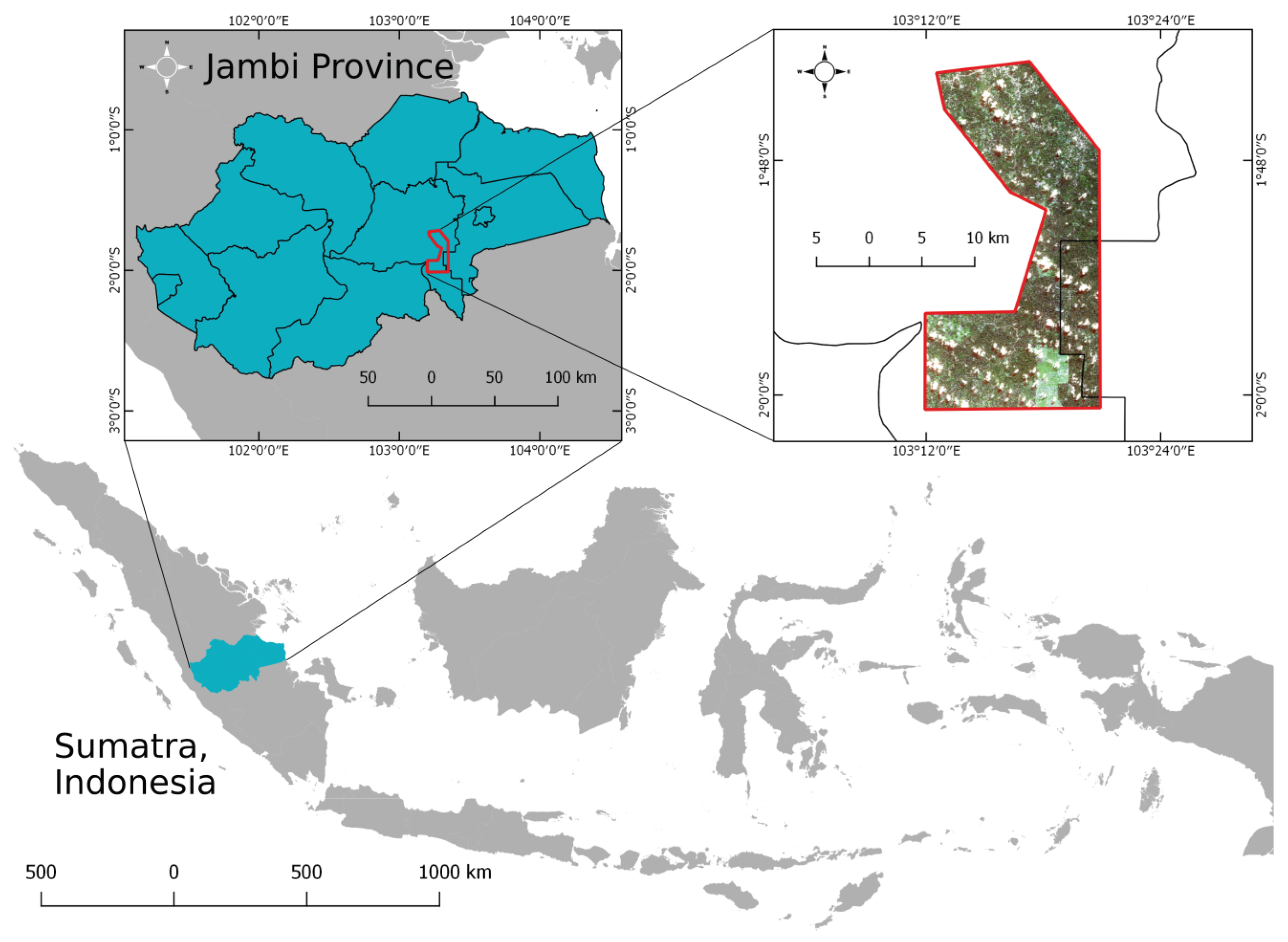
The first study area is located 44 km south-west of Jambi City, Indonesia, and covers an area of about 348 km. It is part of a larger study area of a collaborative research project in the area (CRC990—EEForTS) [24].
In particular, the flat lowland regions of Jambi have seen a dramatic increase in oil palm plantation area over the past decades, which mainly consists of very intensively managed large plantations but also smallholder plantations [25]. In the northern part of the study area, there are mainly smallholder oil palm plantations, with relatively small and loosely grouped patches of remnant forests and villages in between. In the South, large commercial oil palm plantations prevail with several hundreds of thousand of oil palms. There is a big gap in the vegetation cover in the south of the area depicted in the image at the top left of Figure 1, where all palms have been cleared and, in some parts of this gap area, young palms have been re-planted. This is a normal cycle in oil palm management: Old plantations that have passed their stage of high productivity are being removed and replaced by young plants. Accordingly, in larger areas—and also in our dataset—we find palm trees of different age classes and development stages. Younger palms are clearly separated as solitary plants and their crowns are still small. Young palm trees do not yet have the characteristic “star”—shaped arrangement of the leaves when seen from above. As they get older, the palm trees close the gaps between the plants, until the crowns touch and start overlapping.
2.2. Bengaluru, India
Bengaluru, the capital of the Indian State of Karnataka, is located around 1258 N, 7735 E and lies on Southern India’s Deccan plateau at about 920 m above MSL [26]. Founded about in the year 890, Bengaluru is a rapidly growing megapolis with concomitant increases in population (e.g., from 6,537,124 in 2001 to 9,621,551 in 2011) [27]. Before this expansion, Bengaluru was considered the “Garden city” of India, widely known for its beautiful roadside large canopied flowering trees as well as for two large historic parks and botanical gardens [28,29]. Bengaluru is today India’s second fastest growing economy [30]: such economic development triggers a significant influx of population into Bengaluru, which in turn triggers construction activities. The very rapid urban expansion into transition and rural areas has already caused significant losses of tree and vegetation cover in the Bengaluru Metropolitan Region [28,31].
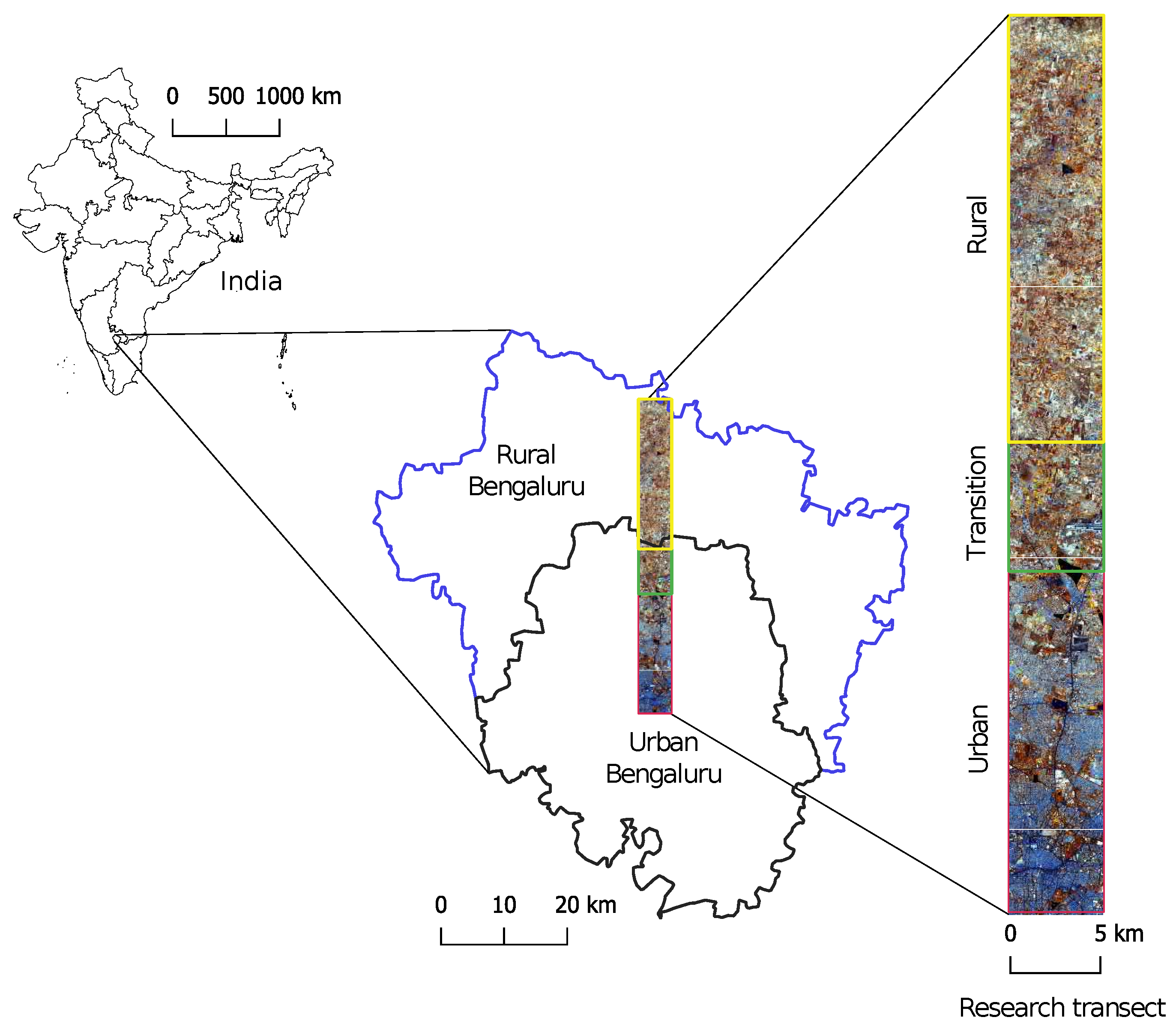
In the framework of a larger Indian-German collaborative research project (FOR2432), a 50 km × 5 km research transect was defined in the northern part of Bengaluru (Figure 2). This transect contains different land-use categories and extends over rural, transition, and urban domains. Contrary to the large monoculture palm oil plantations in Jambi, Bengaluru has coconut palms that are scattered with varying density over the entire study area, where the background also contains buildings, roads, green spaces, or other features.
2.3. Remote Sensing Imagery
The imagery used for the study area of Jambi was acquired on 2 July 2017 by Digital Globe’s WorldView-2 satellite. Apart from large plantations, the images in this dataset contain clouds, shadows, forest, and buildings. The Bengaluru dataset was acquired on 16 November 2016 by WorldView-3 under cloud-free conditions. WorldView-2 has eight multispectral (MS) bands with a nominal resolution of 1.84 m and one panchromatic band with 0.46 m resolution. The difference to WorldView-3, which also has eight bands, is the nominal resolution which is 1.24 m for MS bands and 0.31 m for the panchromatic band. The resolution for WorldView-2 resulting from pansharpening the data is 0.4 m per pixel and for the WorldView-3 imagery we retrieved a resolution of 0.3 m. For pansharpening we used the algorithm implemented in PCI Geomatica 2018 with standard settings. None of the images underwent atmospheric correction, as we want to assess the robustness of our model with respect to dealing with new, raw data.
2.4. Training Data
For generating the training data we first manually digitized the palm tree crown centers. Around these center points, all pixels within a radius of 2 m are then marked as “palm”—this is the ground truth mask. Within the study area in Jambi, we randomly sampled 160 quadratic one hectare plots, wherein a total of 10,679 palms were marked. In addition to that, we marked 4600 non-palm points, which are later used for the training of the classifier (Section 3.5). The training data was collected on the entire dataset, as we are interested in evaluating the accuracy of our model on a large scale.
The Bengaluru training dataset is structured differently: here we selected nine different areas of interest of varying sizes (between 1 and 60 ha). These tiles were selected with the aim of including as many different contexts as possible (urban/transition/rural). Within those tiles we marked 1124 coconut palms for training and 1418 for testing. During the entire labeling process, different band combinations with different contrasts were used in order to ensure high precision.
3. Methods
3.1. U-Net Architecture
Our approach for localizing palm trees uses the so-called U-Net [23], which is a deep neural network that generates semantic segmentations. It receives an image patch and produces a probability map (segmentation) for predefined classes, here palm and background. The term segmentation here refers to the probability map, not to a grouping of pixels as it is often done in remote sensing. The segmentation map has the same lateral dimension as the input (e.g., 112 × 112 pixels). Each pixel of the segmentation map quantifies the probability that this pixel belongs to a palm tree. As the prediction quality in the segmentation map deteriorates close to the border, the output is here cropped by 16 pixels from each edge. In contrast to this architecture, the classifiers used in earlier work (e.g., [17]) output a single number per input image patch, which quantifies the probability that the patch contains a palm.
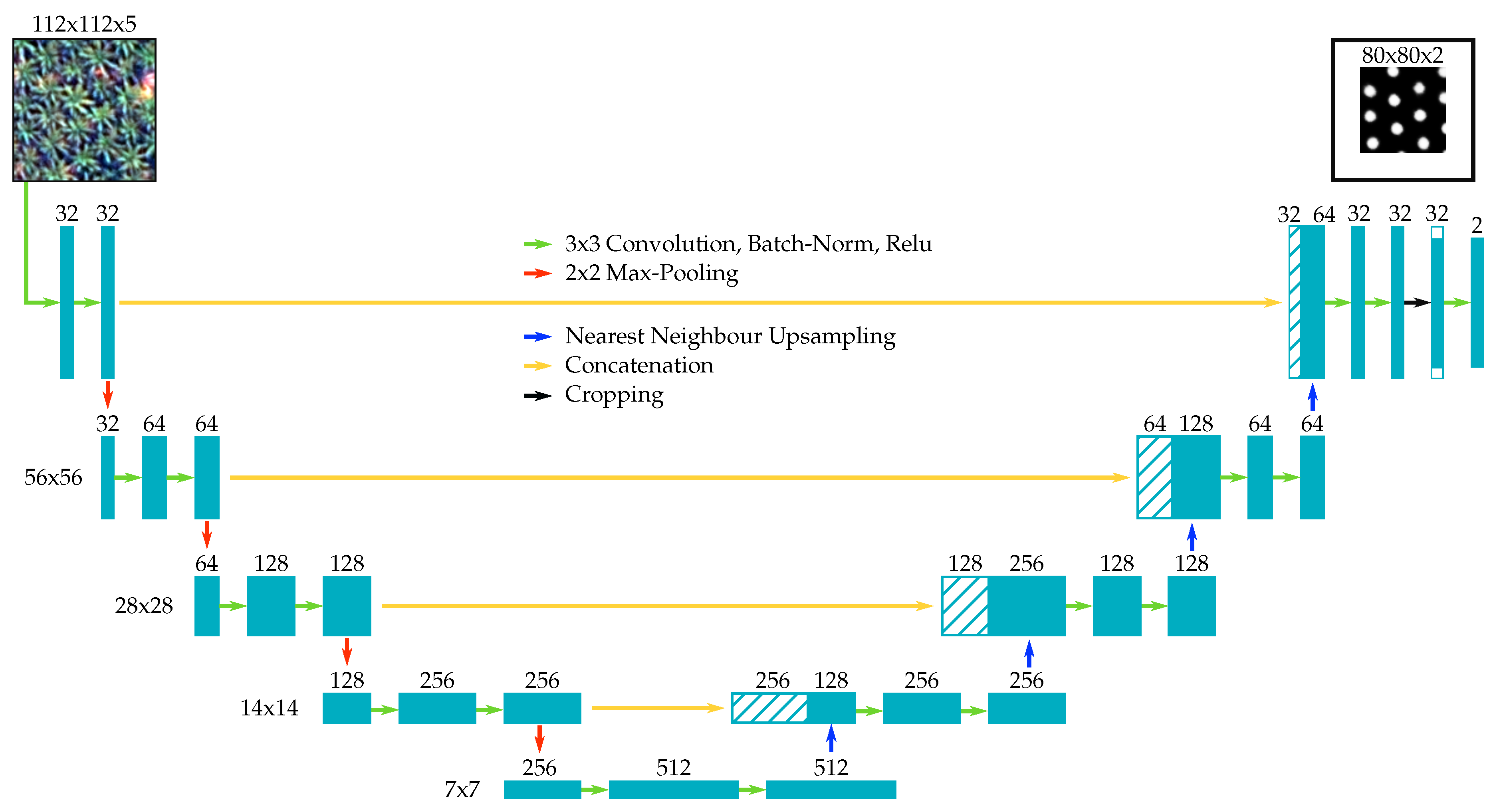
We use two U-Nets (A and B), which differ in certain parameters. U-Net A (Figure 3) is based on [7], which is a complex architecture with proven performance in other tasks. We ported the implementation of Iglovikov et al. [7] to Keras [32] with TensorFlow [33] as back end and made slight modifications to it. The U-Net A comprises five stages. At each stage two 3 × 3 convolution operations are applied, each followed by batch normalization and the ReLU activation. The downsampling between the stages is performed by 2 × 2 pooling operations and—in contrast to the original implementation—we use nearest neighbor upsampling in the expanding part of the network, instead of transposed convolutions. The second adaptation we made is that batch normalization is only used in the contracting part of the network. With these changes we were able to increase the speed of the network without decreasing the accuracy. The last convolution has a kernel size of one and is followed by a softmax activation, in order to map the intermediate feature maps to the final probability maps. U-Net A has approximately 7.8 million parameters.
As palm trees have a simple “star”-shape when seen from above, we hypothesized that it is possible to detect them using a simpler model. The rationale behind these simplifications is that we want to achieve a higher throughput. We experimented with different numbers of stages and convolutions, arriving at U-Net B (Figure 4). U-Net B involves four stages with only one convolution per stage. These convolutions also feature less filters than in U-Net A. In this manner, we reduced the number of parameters in U-Net B to 260,000. Our implementation of the AlexNet described by Li et al. [17] has approximately 790,000 parameters. The number of parameters in the U-Nets does not depend on the input image size. On the contrary, for AlexNet, it does. This is why the U-Net can in principle be fed with images of arbitrary size.
As Li et al. [17] use a resolution that differs from ours, we rescaled the model’s input size and the step width. Li et al. worked on imagery with 0.6 m resolution. Ours is 0.4 m, therefore we increased the input size and step width by a factor of 1.5 to 26 and 5, respectively.
The network input, the ground truth masks used for training, the output, and the final result are shown in Figure 5.
3.2. Inference
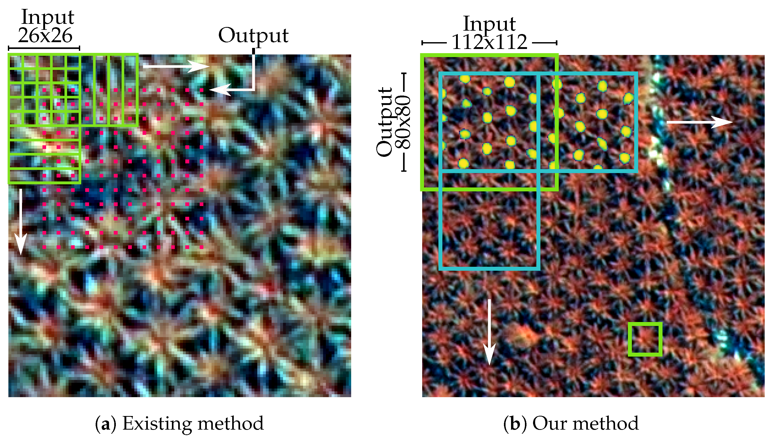
Our approach is comparable to existing ones, in so far as it slides an input window over the area of interest. The difference is that it uses a much larger window size, as can be seen in Figure 6. At each position, an entire segmentation map is produced, instead of a single probability. This allows the detection of several palms at once. Accordingly, the step width can be much larger and far less patches have to be processed.
The network output shown in Figure 5 and Figure 6b is smoothed with a Gaussian filter with a standard-deviation of 1.2 m, which equals 3 or 4 pixels, depending on the dataset. Then we perform a local maximum detection. SciPy’s [34] peak local max function with a minimum distance of 1.2 m, an absolute threshold of 0.15, and a relative threshold of 0.1 is used. The resulting palm positions are then classified as true positive, false positive, or false negative. Peak positions closer than 3.2 m to a true position are counted as true positives, while ensuring that each true palm position can count for only one true positive. Predictions closer than 3.2 m to the global image border were left out of the accuracy assessment in order to avoid boundary effects. The radius of 3.2 m approximately equals two thirds of the crown radius of a full grown palm.
When evaluating the network performance, the inference is done on all images in the test dataset. The true positives, false positives, and false negatives are summed up across all images, then the performance metrics are calculated.
3.3. Quality Measures
The following equations were used to determine accuracy, precision, recall, and -Score of the position detection [35]:
: true positives, : true negatives, : false positives, : false negatives.
A high precision means that each predicted object is a palm, regardless of how many palms were not detected. In contrast, a high recall means that all palms were found, regardless of how many objects were wrongly classified as palm. The F score is the harmonic average of precision and recall.
3.4. Network Training
We trained the two different U-Net architectures A and B on the WorldView-2 imagery in Jambi and evaluated their performance. Apart from that, we benchmarked our method against the existing classifier based on [9,17] with regard to accuracy and computational performance. Then we re-trained and transferred the networks to the WorldView-3 imagery in Bengaluru and assessed their accuracy under these new conditions. Lastly, we utilized the full potential of the U-Net and applied it on a large area. The computer employed was equipped with an Intel Xeon 6136, 96 Gb of memory and two Nvidia GeForce 1080Ti graphics cards, which were both used.
Based on previous experiments, we reduced the original number of bands in both WorldView images to four bands (R, G, B, NIR) and added an additional band: the normalized difference vegetation index (NDVI), so that the network input has five bands in total (R, G, B, NIR, NDVI). Then the images were normalized by subtracting the dataset mean and dividing by the standard deviation for each band separately. The NDVI band remained untouched. In order to train the U-Net, it was fed with randomly cropped image tiles of size 112 × 112 pixels and the corresponding masks in batches of 16 samples. We used random transformations from the Dih symmetry group (the symmetry group of the square; 90 degree rotations and reflections) in order to artificially increase the amount of training data. This process is called data augmentation. A combined loss function of categorical cross entropy and the negative logarithm of the intersection over union of mask and prediction was employed, as described by [7]. We used the Adam optimizer [36] with Nesterov momentum [37].
In order to evaluate the performance of U-Nets A and B on the Jambi dataset, we performed a 10-fold cross validation with a 70–30% split into training and test data. This was necessary because the prediction metrics heavily depend on the selected training and test images. In each run, the network was trained for 600 epochs with 35 steps per epoch. One epoch corresponds to feeding images with a total area equaling the total training area to the network. The initial learning rate was set to 5 × 10 and first lowered to after 350 epochs, then to 5 × 10 after 450 epochs. These parameters correspond to the best performance obtained from empirical evaluations.
3.5. Comparison with Existing Methods
To compare the AlexNet architecture described in [17] with our method, we trained it on the Jambi dataset, again performing a 10-fold cross-validation with exactly the same split into training and test images. Given the dataset size of 11,600 images, the training split of 70%, and the input image size of 26 × 26 pixels, we have approximately 5.5 million pixels available for training. Together with data augmentation, we believe this amount of data is enough to train the 790,000 parameters of AlexNet. Training was done for 100 epochs using a batch size of 16, with 100 steps per epoch, and the same augmentation as before. The initial learning rate was set to and first lowered to after 30 epochs, then to after 50 epochs. This learning rate schedule was optimized by trial and error in order to improve the final network accuracy. We used the categorical cross entropy as loss function and the same optimizer as for the U-Net. The coarse probability maps, resulting from moving the classifier over the test images, were upsampled to match a resolution of 0.4 m. Afterwards, palms were searched with the method described in Section 3.2, the only difference being a threshold value of 0.5 instead of 0.15 for the peak detection. This different threshold was the result of an optimization using nested intervals.
3.6. Speed Benchmark
For an independent performance validation we benchmark our approach against the the approach by Li et al. who used the AlexNet model [38]. This study is the only one that provided the required information about the exact network architecture in our literature revision. All models were tested on the same hardware with the same environment on an image of or pixels. In order to reduce CPU calculation overhead and improve GPU utilization, we transferred the U-Net weights gained from training on pixel tiles to a model with the same architecture but 512 pixels input window size and, therefore, larger output size. In order to test if the increased input window size affects the model accuracy, we performed an evaluation on a subset of 1700 palms. During the benchmark, we neglected the time it took to pre-process the images and took the pure inference time only. The timings were taken after one “warmup” run and averaged over 30 repetitions.
3.7. Transferability of Pre-Trained Network
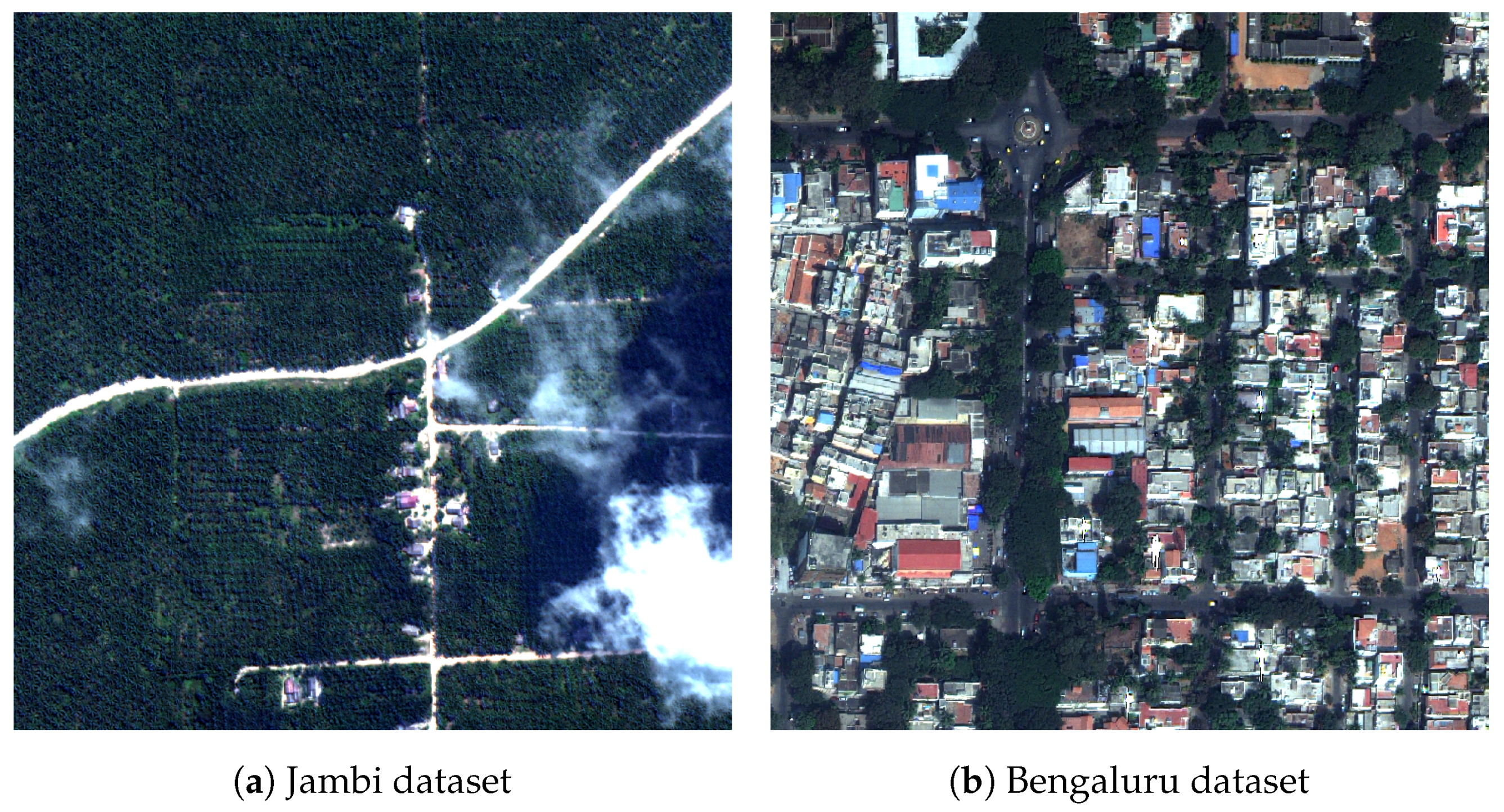
We applied the U-Nets, which had been pre-trained on oil palms in Jambi, to the coconut palm trees in Bengaluru. Both datasets differ slightly in their spatial resolution, as well as in the atmospheric conditions. The environmental contexts in which oil and coconut palms grow, however, are significantly different (Figure 7), and this is the major challenge for the transferability of the network.
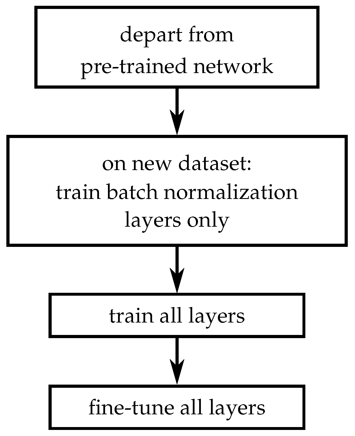
Therefore, directly applying a model pre-trained on one dataset to another may yield bad results. Since collecting massive amounts of new training data was unfeasible, we followed a transfer learning strategy by normalizing the training images. The batch normalization layers in our network learn the mean and standard deviation of the activations on the training dataset, thus they adapt to the color spectrum. In contrast to that, the convolutional layers adapt to low level spatial features and their combination into higher level representations of the data. Since both datasets differ only by 10 cm in resolution, we assumed that the kernels learned by the convolutional layers are still valid. However, the color spectrum changed due to the different atmospheric conditions and varying surface materials. To overcome this, we optimized the batch normalization layers for the new color spectrum, which speeds up the training process. Subsequently, we performed minimal re-training of the entire network. The training procedure comprises three steps (see Figure 8): We departed from a network, which had been pre-trained on the whole WorldView-2 imagery in Jambi for 600 epochs according to the described scheme. In the first step, the learning rate was set to and only the batch normalization layers were trained for 700 gradient updates (which equates to showing 700 image batches to the network, not to confuse with epochs). Second, we trained all layers for 700 gradient updates with a learning rate of . The third step is fine-tuning, which we did for another 700 updates with a learning rate of . The training set contained 1124 palms and the test set 1418. Labeling the 1124 palms in the training dataset took about one to two hours and was therefore considered as an acceptable amount of work for transferring the network.
4. Results
4.1. Classification Accuracy on the Jambi Dataset
Table 1 gives the results for U-Nets A and B, and the classifier approach [17], trained on the Jambi dataset.
The results show that our model outperforms AlexNet. U-Net A scores highest with an accuracy of 88.6%, closely followed by U-Net B, which scores 87.9%. The AlexNet model used in [17] reaches 75%. Detailed curves for the losses and metrics during the training can be found in the Appendix A. Figure 9 sheds some light on the performance of U-Net A under difficult conditions:
4.2. Benchmark and Large Scale Performance
Table 2 lists the results of the speed benchmark, which was done following the procedure described in Section 3.6.
U-Net architecture B is fastest, reaching a throughput of 222.2 ha/s, followed by U-Net A with 121.2 ha/s. The AlexNet [17] reaches a throughput of 22.6 ha/s. Therefore U-Net B is one order of magnitude faster than AlexNet. The speed of the U-Net architecture can be enhanced even more by feeding it with larger image patches, as described in Section 3.6. When feeding image patches with a size of 512 by 512 pixels to the network, U-Net A reaches a throughput of 181.8 ha/s and U-Net B reaches 235.3 ha/s. Increasing the input window size did not affect the accuracy: U-Net A detects 96.1% and U-Net B 92.8% of the 1700 palms the test set created for this task.
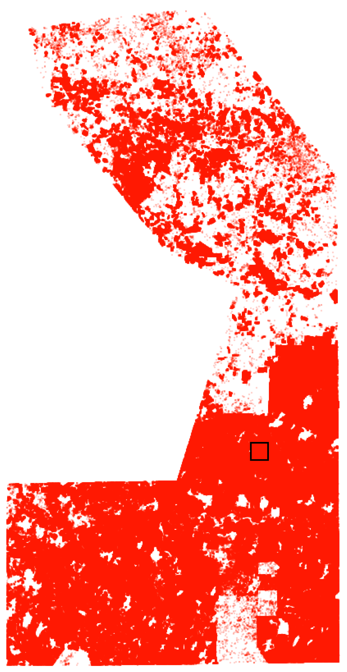
As we have shown the performance in terms of quality and speed, we unleashed the full potential of the U-Net and applied it to the entire dataset. In order to do so, we applied U-Net A as a moving window, as shown in Figure 6. Inference on the whole Jambi dataset of 348 takes 18 min and yields a number of approximately 2.1 million palms. This is slower than one would expect from the numbers in Table 2 due to the non-rectangular shape of our dataset and input/output operations. Figure 10 and Figure 11 show the results. We can observe that the entire southern part of the study area (at the bottom of Figure 10) is covered with large monoculture plantations. In combination with the structured plantation pattern, this indicates a corporate land use. On the other hand, plantations in the northern part are smaller and scattered, therefore most likely owned by smallholders.
4.3. Transfer to the Bengaluru Dataset
We transferred both pre-trained U-Net models to the Bengaluru dataset, as described in Section 3.7. First, we re-trained the batch normalization layers, followed by a fine tuning of the whole network. Training only the batch normalization layers boosted the accuracy from 12% to 83% for architecture A and from 20% to 78% for architecture B. After the subsequent fine-tuning of all layers, architecture A reaches an accuracy of 84.4% and architecture B reaches 91.8%. The entire re-training procedure took only about eight minutes. The final results are summarized in Table 3.
The result of the fine-tuning of U-Net architectures A and B showed that U-Net B performed best on the WorldView-3 Bengaluru dataset. To assess the validity of the approach, we applied it to the whole transect; the resulting map shows approximately 106,000 palm trees. In the urban area, coconut palms are found scattered alongside roads, in parks or gardens, as already found by visual inspection. Further north, in the transition and rural region, palms mainly grow in plantations with only few solitary palm trees. The plantations are much smaller than those in Jambi and the planting distance is larger. Figure 12 shows two examples from the Bengaluru study site:
4.4. Failure Cases
The visual inspection reveals different cases in which the network fails, equally applicable to both architectures. Figure 13 presents examples for the study area of Jambi and Figure 14 refers to the Bengaluru study site.
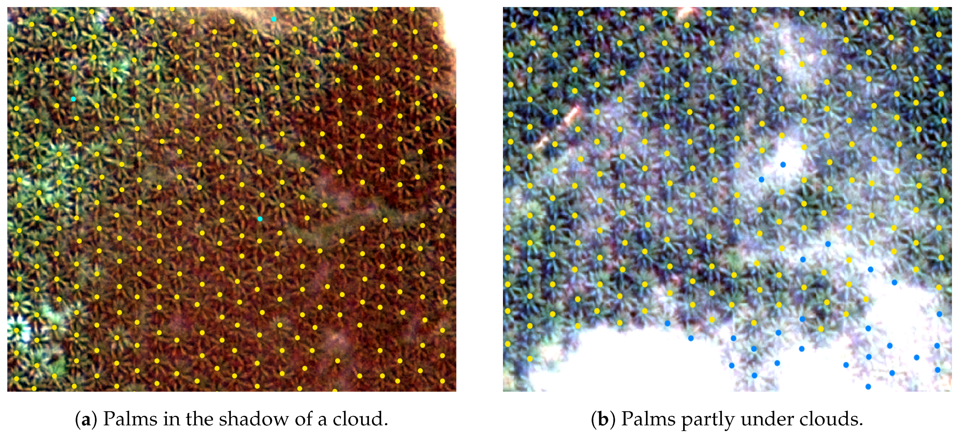
Figure 13a reveals that the network has problems finding young palms in shadows, which is the most common failure case in the Jambi dataset. Shadow is a common factor that also deteriorates the performance in other experiments. Under low light conditions, the network generates false positives in areas with forest and omits some of the adult trees. Nevertheless, visual inspection shows that the predictions are still quite robust under the influence of shadows (see Figure 9). False positives, such as shown in Figure 13b, are rare. They mostly occur in forest areas, where the vegetation randomly resembles a palm, or near bright-dark transitions involving green color. Clouds are tolerable to a certain degree, as long as the ground is still visible.
Figure 14a depicts false positives next to a bright-dark transition in the Bengaluru area, which shows that this error is not restricted to one dataset. In certain areas with low contrast, such as in Figure 14b, the network also fails to detect some palms correctly. Another failure case in the Bengaluru dataset is that young mango trees are also labeled, as they resemble the round, “blob-like” shape of young palms. Apart from that, the network performance depends on the location: it is worse for mixed terrain with forest or urban areas and best on plantations, where it labels almost every object correctly.
5. Discussion and Conclusions
In this paper we presented a new method for large area oil palm detection on very high resolution satellite images, which is based on the U-Net. Overall, we reach F scores well comparable to the ones reported earlier [9,17]. On our dataset, the U-Net outperforms previous approaches by 10–13 percentage points in terms of accuracy and by 6–8 on the F-score. We hypothesize that this improvement has three reasons: First, the U-Net sees the entirety of the training images during the training, while the classifiers in [9,17] only see the cutouts around the palm- or non-palms positions. Therefore, the U-Net effectively sees more training data from the same image source. Second, the U-Net is able to take larger contexts into account during segmentation. It “sees” not only one palm, but several palms. This way, it can for example recognize plantation patterns and adjust the segmentation accordingly. Third, the U-Net is a more powerful network than the AlexNet or LeNet used in [9,17,18] since its internal structure suits the given task better, as it directly highlights the patterns it has been trained for and returns a probability map. Furthermore, U-Net B has 260,000 parameters in comparison to the 790,000 of our AlexNet implementation, so it is also smaller.
Another important contribution of our approach is the computational efficiency, which comes from predicting entire segmentation maps instead of single probabilities, as well as from better utilizing the parallel computing capacity of graphics cards. Our method is able to reduce the computation time by an order of magnitude compared to the existing method, which enabled us to scan areas of several hundred square km within a reasonable amount of time and processing effort—without being restricted to pre-delineated plantations. As our Jambi dataset was collected in a large area, we were able to prove that the U-Net delivers high accuracy even on large scale. Furthermore, the U-Net is well-scalable and able to leverage the performance benefits from newer hardware generations, which would allow to increase the input window size even further.
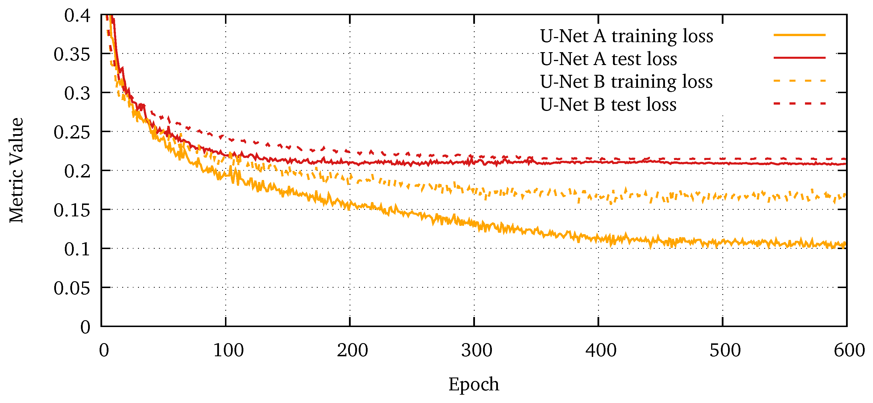
We showed that it is possible to transfer a pre-trained model from one dataset to another with a reasonable amount of new training data. From our two models, the simpler one (U-Net B) had a higher performance on the new dataset (see Table 3). This might be due to the fact that it has less parameters and is therefore less prone to overfitting (see Figure A2). The high accuracy after training the batch normalization layers proves that they play a key role in transferring the model. Atmospheric correction has not been used, as we wanted to assess how well the models generalize to new, raw data. Further studies have to be conducted in order to find out which role atmospheric correction can play in the process of palm detection.
Even though the accuracy of the new method is high, there were some failure cases. The results showed that the models fail when the signal to noise ratio becomes too low, which is the case in dark shadows or at the edges of clouds. In contrast, we have observed that lighter shadows or clouds had only little influence on the results, even though further research has to be conducted in order to verify this capability of our approach. The most common failure, young palms in shadows, has a minor effect on the overall accuracy, as they are rare in the dataset. This failure case could probably be ameliorated by acquiring more training data for this specific class. With respect to the high image resolution, we are confident that the datasets we generated are of high quality. Nevertheless, labeling errors can always occur and impair both, network training and accuracy assessment.
In spite of the good results obtained with the proposed approach, there is room for improvements and further work. For instance, it would be interesting to explore the combination of the U-Net and the networks in [9,17], by applying them to the palm positions predicted by the U-Net. In this manner, it would be possible to reduce the number of false positives while keeping the computational efficiency. The combination of U-Net and classifier could also be used to provide an alternative to existing methods for the classification of diseased trees [39,40].
To conclude, we would like to point out that, thanks to its computational efficiency, our approach may provide an efficient instrument for precisely monitoring palm trees at the level of entire states or even countries, which would at this resolution be impractical with other existing methods.
Author Contributions
Software, methodology and writing—original draft preparation, M.F.; writing—original draft, review and editing, N.N.; supervision, writing—review and editing, A.A.; writing—review, K.U.; supervision, writing—review and editing, F.W. and C.K.
Funding
This research was in part funded by the German Research Foundation, DFG, through grant number KL894/23-1 as part of the Research Unit FOR2432/1 and through grant number 192626868—SFB990 in the framework of the collaborative German—Indonesian research project CRC990.
Acknowledgments
We thank the reviewers for the valuable comments they provided. We are also thankful for the cooperation and infrastructural support provided by our Indian partners at the Institute of Wood Science and Technology (IWST), Bengaluru. We thank the following persons and organizations for granting us access to and use of their properties: village leaders, PT Humusindo, PT REKI. We also thank DigitalGlobe for providing the images as part of the participation at the WorldView Global Alliance Conference 2017.
Conflicts of Interest
The authors declare no conflict of interest. The founding sponsors had no role in the design of the study; in the collection, analyses, or interpretation of data; in the writing of the manuscript, and in the decision to publish the results.
Appendix A
Figure A1.
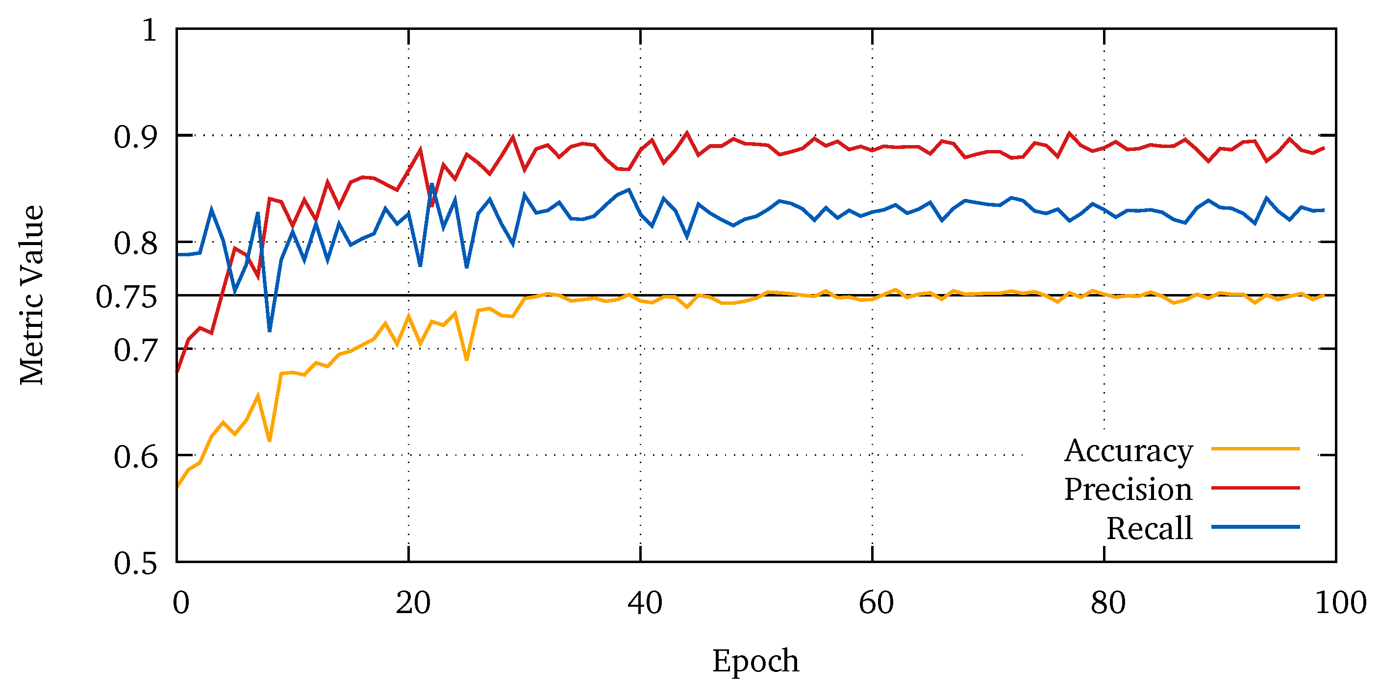
Test accuracy, precision, and recall of architecture A on the Jambi dataset. The graphs show the metrics derived from the predicted positions averaged over all k-fold runs. The curves for U-Net B look similar.
Figure A1.
Test accuracy, precision, and recall of architecture A on the Jambi dataset. The graphs show the metrics derived from the predicted positions averaged over all k-fold runs. The curves for U-Net B look similar.

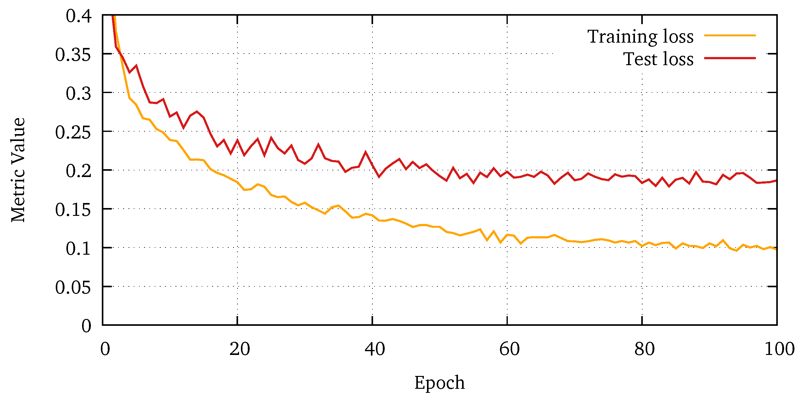
Figure A2.
Training and test loss for U-Net A and B, averaged over 10 cross-validation runs. U-Net B has a lower spread between training and test loss, which indicates that it is less prone to overfitting. This is due to the lower number of parameters (260,000 vs. 7.8 m).
Figure A2.
Training and test loss for U-Net A and B, averaged over 10 cross-validation runs. U-Net B has a lower spread between training and test loss, which indicates that it is less prone to overfitting. This is due to the lower number of parameters (260,000 vs. 7.8 m).

Figure A3.
Test accuracy, precision, and recall for the AlexNet classifier [17], averaged over all k-fold runs.
Figure A3.
Test accuracy, precision, and recall for the AlexNet classifier [17], averaged over all k-fold runs.

Figure A4.
Categorical cross entropy loss of the classifier.

References
- Corley, R. How much palm oil do we need? Environ. Sci. Policy 2009, 12, 134–139. [Google Scholar] [CrossRef]
- Singh, S.R.M. India to become the global leader in coconut production and productivity. Available online: http://www.pib.nic.in/Pressreleaseshare.aspx?PRID=1517947/ (accessed on 3 December 2018).
- Food and Agriculture Organization of the United Nations (FAO), FAO Office for Asia and the Pacific and Asia Pacific Coconut Community (APCC). Report of the FAO High Level Expert Consultation on Coconut Sector Development in Asia and the Pacific Region; FAO: Roma, Italy, 2014. [Google Scholar]
- Zhu, X.X.; Tuia, D.; Mou, L.; Xia, G.; Zhang, L.; Xu, F.; Fraundorfer, F. Deep Learning in Remote Sensing: A Comprehensive Review and List of Resources. IEEE Geosci. Remote Sens. Mag. 2017, 5, 8–36. [Google Scholar] [CrossRef]
- Zhang, L.; Zhang, L.; Du, B. Deep learning for remote sensing data: A technical tutorial on the state of the art. IEEE Geosci. Remote Sens. Mag. 2016, 4, 22–40. [Google Scholar] [CrossRef]
- Kussul, N.; Lavreniuk, M.; Skakun, S.; Shelestov, A. Deep learning classification of land cover and crop types using remote sensing data. IEEE Geosci. Remote Sens. Lett. 2017, 14, 778–782. [Google Scholar] [CrossRef]
- Iglovikov, V.; Mushinskiy, S.; Osin, V. Satellite Imagery Feature Detection using Deep Convolutional Neural Network: A Kaggle Competition. arXiv, 2017; arXiv:1706.06169. [Google Scholar]
- Scott, G.J.; England, M.R.; Starms, W.A.; Marcum, R.A.; Davis, C.H. Training deep convolutional neural networks for land–cover classification of high-resolution imagery. IEEE Geosci. Remote Sens. Lett. 2017, 14, 549–553. [Google Scholar] [CrossRef]
- Li, W.; Fu, H.; Yu, L.; Cracknell, A. Deep Learning Based Oil Palm Tree Detection and Counting for High-Resolution Remote Sensing Images. Remote Sens. 2016, 9, 22. [Google Scholar] [CrossRef]
- Chong, K.L.; Kanniah, K.D.; Pohl, C.; Tan, K.P. A review of remote sensing applications for oil palm studies. Geo-Spat. Inf. Sci. 2017, 20, 184–200. [Google Scholar] [CrossRef]
- The Forest Trust. All of Nestlé’s Palm Oil Supply Chain to be 100% Satellite Monitored 2018. Available online: http://www.tft-earth.org/stories/news/nestlesatellite/ (accessed on 14 December 2018).
- Greenpeace. How the Palm Oil Industry is Cooking the Climate; Greenpeace: Amsterdam, The Netherlands, 2007. [Google Scholar]
- Tan, K.P.; Kanniah, K.D.; Cracknell, A.P. A review of remote sensing based productivity models and their suitability for studying oil palm productivity in tropical regions. Prog. Phys. Geogr. 2012, 36, 655–679. [Google Scholar] [CrossRef]
- Cheng, Y.; Yu, L.; Cracknell, A.P.; Gong, P. Oil palm mapping using Landsat and PALSAR: A case study in Malaysia. Int. J. Remote Sens. 2016, 37, 5431–5442. [Google Scholar] [CrossRef]
- Tan, K.P.; Kanniah, K.D.; Cracknell, A.P. Use of UK-DMC 2 and ALOS PALSAR for studying the age of oil palm trees in southern peninsular Malaysia. Int. J. Remote Sens. 2013, 34, 7424–7446. [Google Scholar] [CrossRef]
- Srestasathiern, P.; Rakwatin, P. Oil Palm Tree Detection with High Resolution Multi-Spectral Satellite Imagery. Remote Sens. 2014, 6, 9749–9774. [Google Scholar] [CrossRef]
- Li, W.; Fu, H.; Yu, L. Deep convolutional neural network based large-scale oil palm tree detection for high-resolution remote sensing images. In Proceedings of the 2017 IEEE International Geoscience and Remote Sensing Symposium (IGARSS), Fort Worth, TX, USA, 23–28 July 2017; pp. 846–849. [Google Scholar] [CrossRef]
- Koon Cheang, E.; Koon Cheang, T.; Haur Tay, Y. Using Convolutional Neural Networks to Count Palm Trees in Satellite Images. arXiv, 2017; arXiv:1701.06462. [Google Scholar]
- Pouliot, D.; King, D.; Bell, F.; Pitt, D. Automated tree crown detection and delineation in high-resolution digital camera imagery of coniferous forest regeneration. Remote Sens. Environ. 2002, 82, 322–334. [Google Scholar] [CrossRef]
- Ke, Y.; Quackenbush, L.J. A review of methods for automatic individual tree-crown detection and delineation from passive remote sensing. Int. J. Remote Sens. 2011, 32, 4725–4747. [Google Scholar] [CrossRef]
- Shafri, H.Z.M.; Hamdan, N.; Saripan, M.I. Semi-automatic detection and counting of oil palm trees from high spatial resolution airborne imagery. Int. J. Remote Sens. 2011, 32, 2095–2115. [Google Scholar] [CrossRef]
- Koch, B.; Heyder, U.; Weinacker, H. Detection of individual tree crowns in airborne lidar data. Photogramm. Eng. Remote Sens. 2006, 72, 357–363. [Google Scholar] [CrossRef]
- Ronneberger, O.; Fischer, P.; Brox, T. U-Net: Convolutional Networks for Biomedical Image Segmentation. arXiv 2015, arXiv:1505.04597. [Google Scholar]
- Drescher, J.; Rembold, K.; Allen, K.; Beckschäfer, P.; Buchori, D.; Clough, Y.; Faust, H.; Fauzi, A.M.; Gunawan, D.; Hertel, D.; et al. Ecological and socio-economic functions across tropical land use systems after rainforest conversion. Philos. Trans. R. Soc. B Biol. Sci. 2016, 371, 1964. [Google Scholar] [CrossRef]
- Kubitza, C.; Krishna, V.V.; Urban, K.; Alamsyah, Z.; Qaim, M. Land Property Rights, Agricultural Intensification, and Deforestation in Indonesia. Ecol. Econ. 2018, 147, 312–321. [Google Scholar] [CrossRef]
- Sudhira, H.; Nagendra, H. Local assessment of Bangalore: Graying and greening in Bangalore—Impacts of urbanization on ecosystems, ecosystem services and biodiversity. In Urbanization, Biodiversity and Ecosystem Services: Challenges and Opportunities; Springer: Berlin/Heidelberg, Germany, 2013; pp. 75–91. [Google Scholar]
- Directorate of Census Operations, Karnataka. Census of India, 2011; Directorate of Census Operations, Karnataka and Office of the Registrar General & Census Commissioner, India, Ministry of Home Affairs, Govt. of India: Bangalore, India; New Delhi, India, 2011.
- Nagendra, H.; Gopal, D. Street trees in Bangalore: Density, diversity, composition and distribution. Urban For. Urban Green. 2010, 9, 129–137. [Google Scholar] [CrossRef]
- Nair, J. The Promise of the Metropolis: Bangalore’s Twentieth Century; Oxford University Press: New Delhi, India, 2005. [Google Scholar]
- Sudhira, H.; Ramachandra, T.; Subrahmanya, M.B. Bangalore. Cities 2007, 24, 379–390. [Google Scholar] [CrossRef]
- Nagendra, H.; Nagendran, S.; Paul, S.; Pareeth, S. Graying, greening and fragmentation in the rapidly expanding Indian city of Bangalore. Landsc. Urban Plan. 2012, 105, 400–406. [Google Scholar] [CrossRef]
- Chollet, F. Keras, 2015. Available online: https://keras.io (accessed on 1 July 2018).
- Abadi, M.; Agarwal, A.; Barham, P.; Brevdo, E.; Chen, Z.; Citro, C.; Corrado, G.S.; Davis, A.; Dean, J.; Devin, M.; et al. TensorFlow: Large-Scale Machine Learning on Heterogeneous Systems, 2015. Available online: tensorflow.org (accessed on 1 July 2018).
- Jones, E.; Oliphant, T.; Peterson, P. SciPy: Open source scientific tools for Python, 2001. Available online: https://www.scipy.org/ (accessed on 1 July 2018).
- Nevalainen, O.; Honkavaara, E.; Tuominen, S.; Viljanen, N.; Hakala, T.; Yu, X.; Hyyppä, J.; Saari, H.; Pölönen, I.; Imai, N.; et al. Individual Tree Detection and Classification with UAV-Based Photogrammetric Point Clouds and Hyperspectral Imaging. Remote Sens. 2017, 9, 185. [Google Scholar] [CrossRef]
- Kingma, D.P.; Ba, J. Adam: A Method for Stochastic Optimization. arXiv, 2014; arXiv:1412.6980. [Google Scholar]
- Dozat, T. Incorporating Nesterov momentum into Adam. ICLR Workshop, 2016. [Google Scholar]
- Krizhevsky, A.; Sutskever, I.; Hinton, G.E. Imagenet classification with deep convolutional neural networks. In Advances in Neural Information Processing Systems; MIT Press: Cambridge, MA, USA, 2012; pp. 1097–1105. [Google Scholar]
- Shafri, H.Z.; Hamdan, N. Hyperspectral imagery for mapping disease infection in oil palm plantationusing vegetation indices and red edge techniques. Am. J. Appl. Sci. 2009, 6, 1031. [Google Scholar]
- Santoso, H.; Gunawan, T.; Jatmiko, R.H.; Darmosarkoro, W.; Minasny, B. Mapping and identifying basal stem rot disease in oil palms in North Sumatra with QuickBird imagery. Precis. Agric. 2011, 12, 233–248. [Google Scholar] [CrossRef]
Figure 1.
The first study site is located 44 km south-west of Jambi City, Indonesia.

Figure 2.
The research transect is located in the northern part of Bengaluru and, as the left map shows, lies partly in the administrative regions “Urban Bengaluru” and partly in “Rural Bengaluru”. Our own breakdown into the three domains “rural”, “transition”, and “urban” follows the percentage of built-up area and is illustrated by differently colored frames around the transect sections (yellow for “rural”, green for “transition”, and red for “urban”). The transect is enlarged here as a false color composite.

Figure 3.
U-Net architecture A. The U-Net has a “contracting” (left) and an “expanding” part (right). Information from earlier layers is fused with the output of later layers, which improves the accuracy of the segmentation. The last convolution has a kernel size of one.
Figure 3.
U-Net architecture A. The U-Net has a “contracting” (left) and an “expanding” part (right). Information from earlier layers is fused with the output of later layers, which improves the accuracy of the segmentation. The last convolution has a kernel size of one.

Figure 4.
U-Net architecture B. This is a simpler version of U-Net A and is optimized for speed. The last convolution has a kernel size of one.
Figure 4.
U-Net architecture B. This is a simpler version of U-Net A and is optimized for speed. The last convolution has a kernel size of one.

Figure 5.
The network directly generates a “palm probability map” (c) from the input image (a), locating several instances (palms) at once. The output is smaller, because we crop 16 pixels from each edge. This output is optimized in order to best match the ground truth mask (b). The maxima in the smoothed probability map correspond to the identified palm positions. The final result is shown in (d) with yellow dots as true positives.

Figure 6.
In (a) the existing method is shown (e.g., [9]). A classifier window (green) is moved across the image in steps of a few pixels. At each position (red), the classifier calculates a “palm probability”, from which a coarse probability map is created. In our method (b), the input window (green) is moved over the image in larger steps. At each position, the segmentation is calculated. The output window (blue) is slightly smaller than the input, because it is cropped due to the lower prediction quality at the borders. The palm positions can then be inferred from each probability map. The small rectangle at the bottom of (b) has the size of the classifier input in [9], scaled up to match our image resolution (26 × 26 pixels).

Figure 7.
Sample images from the two datasets.

Figure 8.
The transfer procedure comprises three steps: exclusive training of the batch normalization layers, full network training, and fine-tuning.
Figure 8.
The transfer procedure comprises three steps: exclusive training of the batch normalization layers, full network training, and fine-tuning.

Figure 9.
The network still detects palms under difficult conditions. True positives are marked yellow and false negatives blue.
Figure 9.
The network still detects palms under difficult conditions. True positives are marked yellow and false negatives blue.

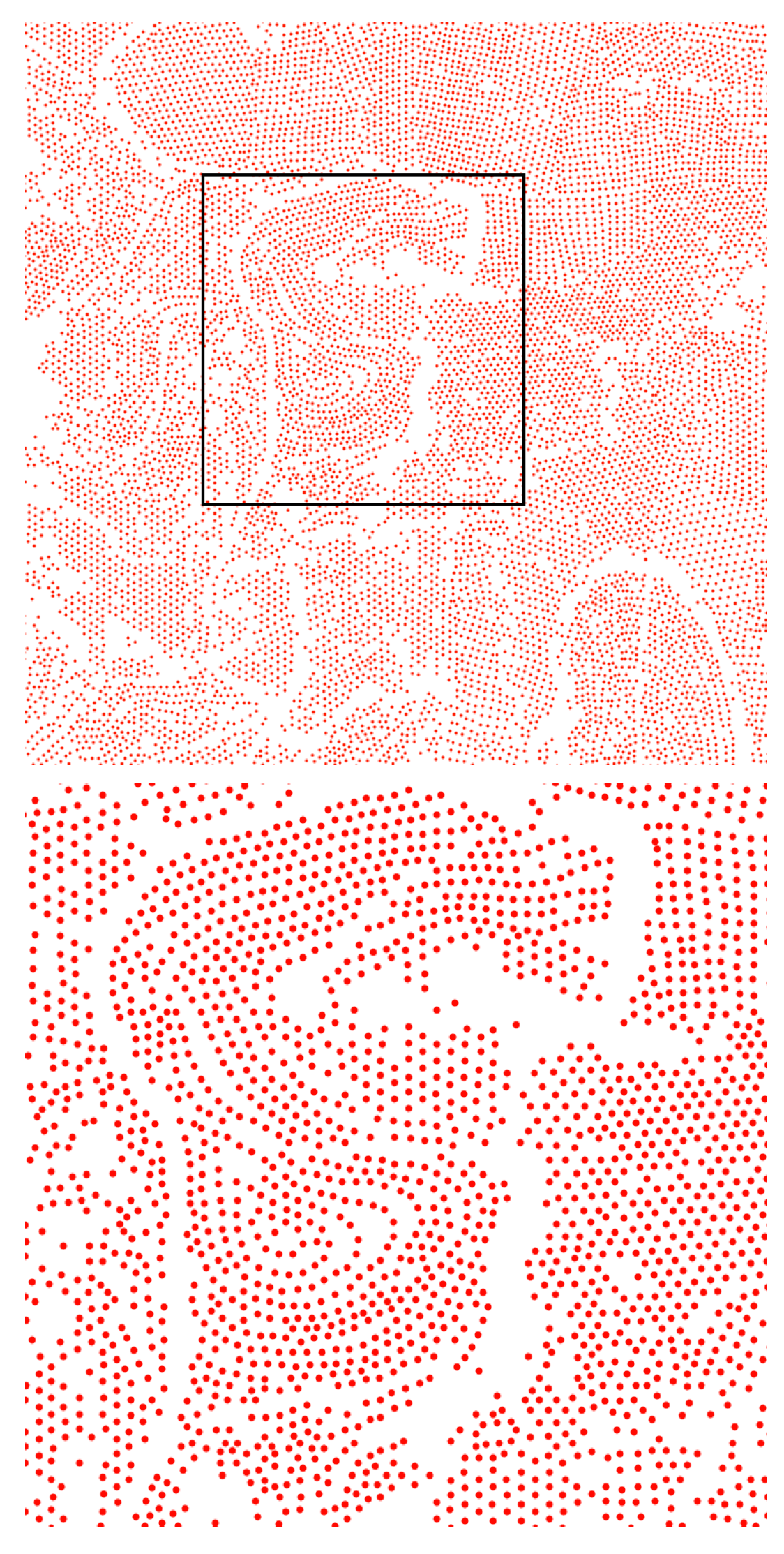
Figure 10.
The palm coverage of the Jambi study site. The image displays 2.1 million palms, each one resolved individually.
Figure 10.
The palm coverage of the Jambi study site. The image displays 2.1 million palms, each one resolved individually.

Figure 11.
Zoom into the study site. The magnification increases from top to bottom. With higher magnification, the planting patterns become clear.
Figure 11.
Zoom into the study site. The magnification increases from top to bottom. With higher magnification, the planting patterns become clear.

Figure 12.
Samples from the Bengaluru study area after transferring U-Net B. True positives are marked yellow and false positives red.
Figure 12.
Samples from the Bengaluru study area after transferring U-Net B. True positives are marked yellow and false positives red.

Figure 13.
Failure cases in the Jambi study area: True positives are marked in yellow, false positives in red, and false negatives in blue. Young palms in shadows are rare in the dataset, and therefore hardly detected. Other failure cases, such as in (b), are challenging to find, as they rarely occur.

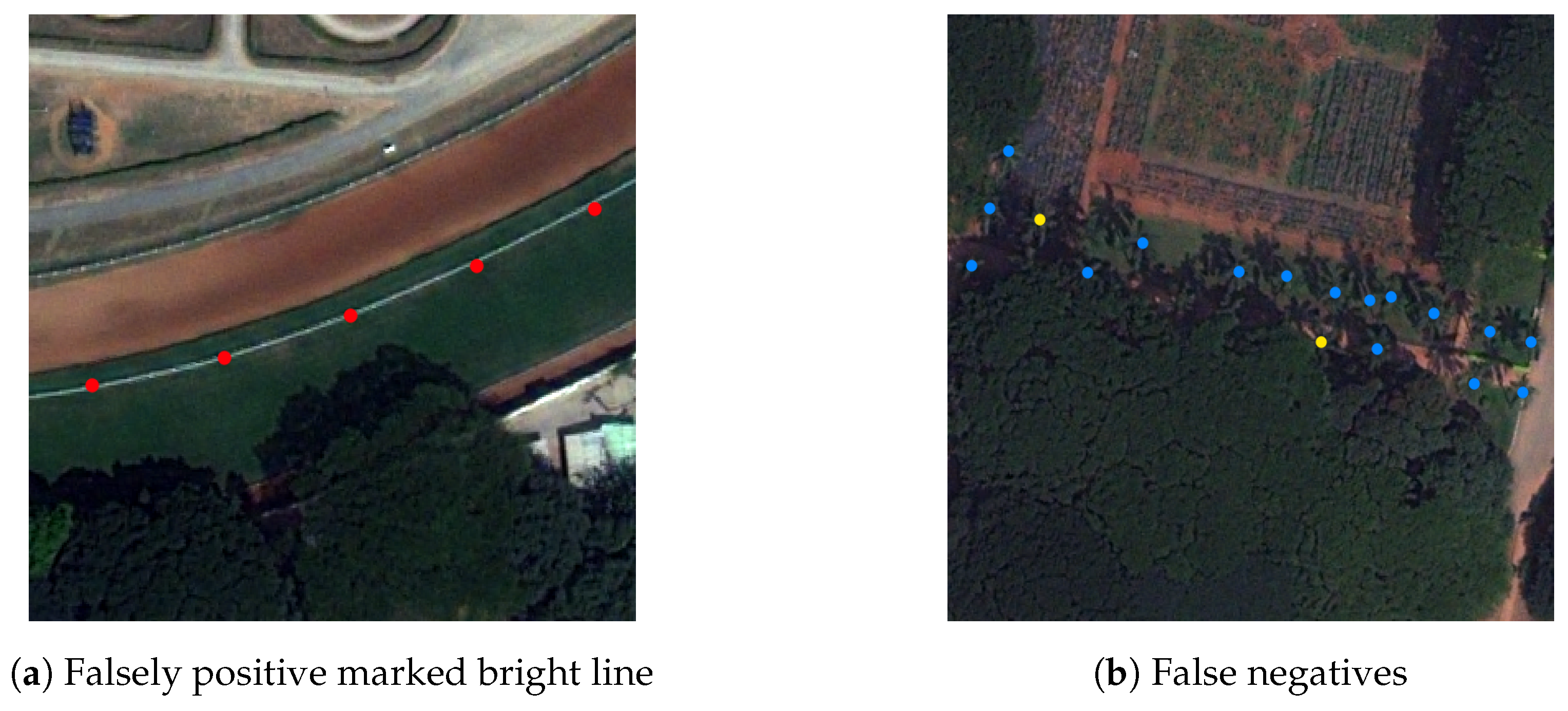
Figure 14.
Failure cases in the study area of Bengaluru. True positives are marked yellow, false positives red, and false negatives blue. In (a) the convolutional filters respond to a bright line. In (b) the network fails to detect some palm trees probably because of dark green grass in the background.


Table 1.
Performance metrics of our model in comparison with state of the art method. The numbers have been obtained by first averaging over the k-fold runs and then averaging over the last 50 epochs, after the metrics have converged. Highest numbers are highlighted. The training history is given in the Appendix A.
| Accuracy | Precision | Recall | -Score | |
|---|---|---|---|---|
| U-Net A | 88.6% | 94.4% | 93.5% | 93.9% |
| U-Net B | 87.9% | 93.2% | 94.0% | 93.6% |
| AlexNet [17] | 75.0% | 88.8% | 83.0% | 85.8% |
Table 2.
Results of the speed benchmark. The standard deviations for the timings were 0.08 s for AlexNet, 0.05 s for U-Net A, and 0.03 s for U-Net B.
Table 2.
Results of the speed benchmark. The standard deviations for the timings were 0.08 s for AlexNet, 0.05 s for U-Net A, and 0.03 s for U-Net B.
| Network | Input Size [px] | Step [px] | Time [s] | Throughput [ha/s] |
|---|---|---|---|---|
| AlexNet [17] | 5 | 17.7 | 22.6 | |
| U-Net A | 80 | 3.3 | 121.2 | |
| U-Net B | 80 | 1.8 | 222.2 |
Table 3.
Performance metrics for the two architectures after training the batch normalization layers only, and for the full transfer. Here the metrics have been derived from a set of test images and not from k-fold validation. Highest numbers are highlighted.
Table 3.
Performance metrics for the two architectures after training the batch normalization layers only, and for the full transfer. Here the metrics have been derived from a set of test images and not from k-fold validation. Highest numbers are highlighted.
| Accuracy | Precision | Recall | -Score | |
|---|---|---|---|---|
| U-Net A BN only | 83.3% | 86.9% | 95.2% | 90.9% |
| U-Net B BN only | 77.8% | 83.1% | 92.4% | 87.5% |
| U-Net A | 84.4% | 88.6% | 94.7% | 91.6% |
| U-Net B | 91.8% | 95.0% | 96.4% | 95.7% |
© 2019 by the authors. Licensee MDPI, Basel, Switzerland. This article is an open access article distributed under the terms and conditions of the Creative Commons Attribution (CC BY) license (http://creativecommons.org/licenses/by/4.0/).
Share and Cite
MDPI and ACS Style
Freudenberg, M.; Nölke, N.; Agostini, A.; Urban, K.; Wörgötter, F.; Kleinn, C. Large Scale Palm Tree Detection in High Resolution Satellite Images Using U-Net. Remote Sens. 2019, 11, 312. https://doi.org/10.3390/rs11030312
AMA Style
Freudenberg M, Nölke N, Agostini A, Urban K, Wörgötter F, Kleinn C. Large Scale Palm Tree Detection in High Resolution Satellite Images Using U-Net. Remote Sensing. 2019; 11(3):312. https://doi.org/10.3390/rs11030312
Chicago/Turabian StyleFreudenberg, Maximilian, Nils Nölke, Alejandro Agostini, Kira Urban, Florentin Wörgötter, and Christoph Kleinn. 2019. "Large Scale Palm Tree Detection in High Resolution Satellite Images Using U-Net" Remote Sensing 11, no. 3: 312. https://doi.org/10.3390/rs11030312
Note that from the first issue of 2016, this journal uses article numbers instead of page numbers. See further details here.