1. Introduction
Oil spill pollution on the sea surface is harmful to marine ecosystems, fisheries, wildlife, and other societal interests. Scientists and researchers have made a great effort to monitor oil spills on the sea surface. Many scientific papers covering a wide range of topics have written about the used means of monitoring of oil spills, e.g., Salberg et al. [
1], Skunes et al. [
2], Lupidi et al. [
3], etc. It is well-known that the synthetic aperture radar (SAR) is almost independent of atmospheric conditions, and can provide high-resolution measurements at both day and night [
4]. It has been proven that SAR is a useful tool for ocean remote sensing, especially for oil spill detection and monitoring. In previous literature, the problem of oil spill monitoring has been studied mainly from two aspects. The first one focuses on detecting oil spills by using measured SAR images [
5,
6,
7,
8,
9,
10,
11]. The second one focuses on analyzing electromagnetic (EM) field scattered from clean and polluted sea surfaces [
12,
13,
14,
15]. Unlike previous papers, the motivation of this work is to investigate the influences caused by slicks on sea surface characteristics and the EM scattering from slick-covered and slick-free sea surfaces, both theoretically as well as experimentally.
The influences caused by slicks can mainly be described by two effects: the damping of small-scale sea waves, and the reduction of friction velocity. On one hand, due to the damping effects for short-gravity and capillary waves, the sea surface profile of the slick-covered sea surface is quite different from that of the slick-free surface. The damping effect is usually described by the Marangoni theory [
16]. On the other hand, as a slick-covered surface is smoother, the friction velocity is reduced, and the energy transferred from the wind to sea waves is also reduced. These two effects will both directly influence the sea height spectrum.
For the EM scattering from sea surface, the backscattered field depends on the sea roughness state. In the past decades, various approximate methods have been developed for the estimation of the EM scattering field from rough sea surface. Among these methods, the Kirchhoff approximation (KA) [
17], the small perturbation method (SPM) [
18], and the two-scale model (TSM) are effective methods for estimating the scattering coefficient. Unfortunately, all these three methods are only available in certain conditions or involve a cutoff parameter to separate sea waves into small and large scales. The small slope approximation (SSA) is a unified model that is suitable for large-scale, intermediate-scale, and small-scale roughness surfaces under the condition that the tangent of grazing angles of incident/scattered waves sufficiently exceeds the root mean square (RMS) slope [
19,
20]. According to the requirement of accuracy, the SSA can be divided into the first-order SSA (SSA-1) and the second order SSA (SSA-2). The SSA-1 involves less computation, but it cannot provide cross-polarized (HV or VH) scattering coefficient estimation in backscatter configurations. In contrast, the SSA-2 does not involve any arbitrary parameters and it could provide predictions for cross-polarized scattering coefficient estimation. To our knowledge, the SSA-2 has never been used to study the EM scattering from both slick-free and slick-covered sea surfaces. The main contribution of this work is to study EM scattering from sea surfaces covered with and without slick, both theoretically and experimentally.
This paper is organized as follows: the theoretical derivations of the damping model and the SSA-2 are briefly reviewed in
Section 2. Numerical simulations of normalized radar cross-sections (NRCSs) of slick-free and slick-covered sea surfaces are presented and discussed in
Section 3. Finally, conclusions and perspective are drawn in
Section 4.
2. Theory and Methodology
2.1. The Damping Model
The influences of the slick can mainly induce by two effects, i.e., the damping effect for small-scale sea waves, and the reduction of friction velocity. In general, the damping effect caused by slick is modeled by the Marangoni theory [
13,
21]. The damping ratio induced by slick can be expressed as:
where
τ,
X, and
Y are given as:
In Equation (1),
kw is the wavenumber of sea waves,
ω is the angular frequency of sea waves,
is dynamic viscosity, and
ρ is the density of seawater, respectively.
E0 denotes the elasticity modulus, and
is a characteristic pulsation. In this work, we investigate two kinds of slicks, which are denoted as slick-a (
E0 = 9 mN/s,
ωD = 6 rad/s) and slick-b (
E0 = 25 mN/s,
ωD = 11 rad/s), and correspond to organic films measured in two cases. These values were retrieved from field experiments, and have been used in previous works for studying the impacts of slicks on EM scattering field from sea surface [
12,
13]. It should be noted that this model does not involve the thickness of slick.
Besides, given that the slick film may be partially dispersed by the winds and the sea waves, a fractional filling factor
F is introduced to modify the damping ratio. Finally, the damping ratio can be written as [
13]:
Obviously, the damping model is homogeneous, which implies that the damping effect is not associated with wind direction.
As the small-scale waves of the slick-covered surface are damped, the roughness of the surface is reduced. As a consequence, the energy transferred from the wind to sea waves, which is related to the friction velocity, is reduced. This phenomenon has been observed in field experiments: the friction velocity of the slick-covered surface is smaller than the slick-free surface. The friction velocity of a slick-covered surface
can be calculated empirically with [
22]:
where
. In this work, the value of
suggested by Gade et al. is adopted [
23]; i.e.,
β = 0.7. Thus, the spectrum of sea surface covered by slick is related to the clean sea surface spectrum by:
where
denotes the spectrum covered by slick, and
denotes the clean sea surface spectrum.
2.2. The Second-Order Small Slope Approximation (SSA-2)
According to the theory of small slope approximation, the scattering amplitude of the second order can be written as [
19,
20]:
The incoherent scattering amplitude can be calculated with
. The incoherent scattering coefficient can be calculated with the incoherent scattering amplitude by:
The meanings of the parameters in the equations above can be found in the
Appendix A. As shown in Equation (6), the calculation of scattering amplitude of the SSA-2 is rather complex, as it requires the calculation of a fourfold integral. This involves a large amount of computation, and it takes a long time to perform the numerical simulation, which is the main drawback of the SSA-2. For more details about the numerical simulations mentioned above, please refer to
Appendix A.
Additionally, to model the seawater dielectric constant, the Debye model is employed in all simulations, where the temperature equals 20 °C, and the salinity equals 35 ppt. For microwave scattering, the dielectric constant of the oil is much smaller than seawater; the oil layer can be regarded as a “transparent” layer. That is to say, the EM scattering energy is mainly contributed by the seawater under oil. Besides, the thickness of a surface film (either a monomolecular slick or a thin oil spill) is small compared with the penetration depth of microwaves into the water. Thus, in numerical simulation, the impact induced by the dielectric constant of slick has been neglected [
23].
3. Numerical Simulations and Discussions
3.1. Impacts of Slick on the Sea Surface
The EM scattering field is highly dependent on the characteristics of the rough surface. To study the EM scattering from the slick-covered sea surface, it is necessary to make how the slick influences the sea surface clear. Therefore, in this part, the impacts of slicks on a clean sea surface are simulated and discussed from several aspects, including the sea curvature spectrum, the RMS height, RMS slope, and the autocorrelation function.
3.1.1. The Damping Ratio for Various Bands
According to
Section 2, the damping ratio can be calculated with Equation (3).
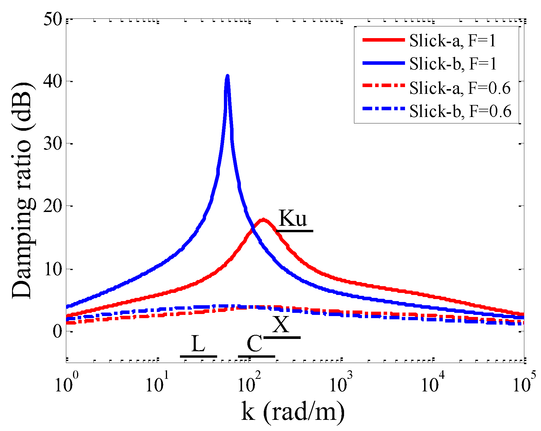
Figure 1 displays the damping ratios of two kinds of slicks.
In
Figure 1, it is observed that the damping ratios first increase, and then decrease with sea wavenumber. There exist peak values for both kinds of slicks. For about
k <100 rad/m, slick-b has a larger damping ratio, while for about
k >100 rad/m, slick-a has a larger damping ratio. The damping effect becomes more significant with a larger fractional filling parameter
F. According to Bragg scattering theory, the Bragg wavenumber of sea surface can be written as:
where
ke is the electromagnetic wavenumber, and
θi is the incident angle.
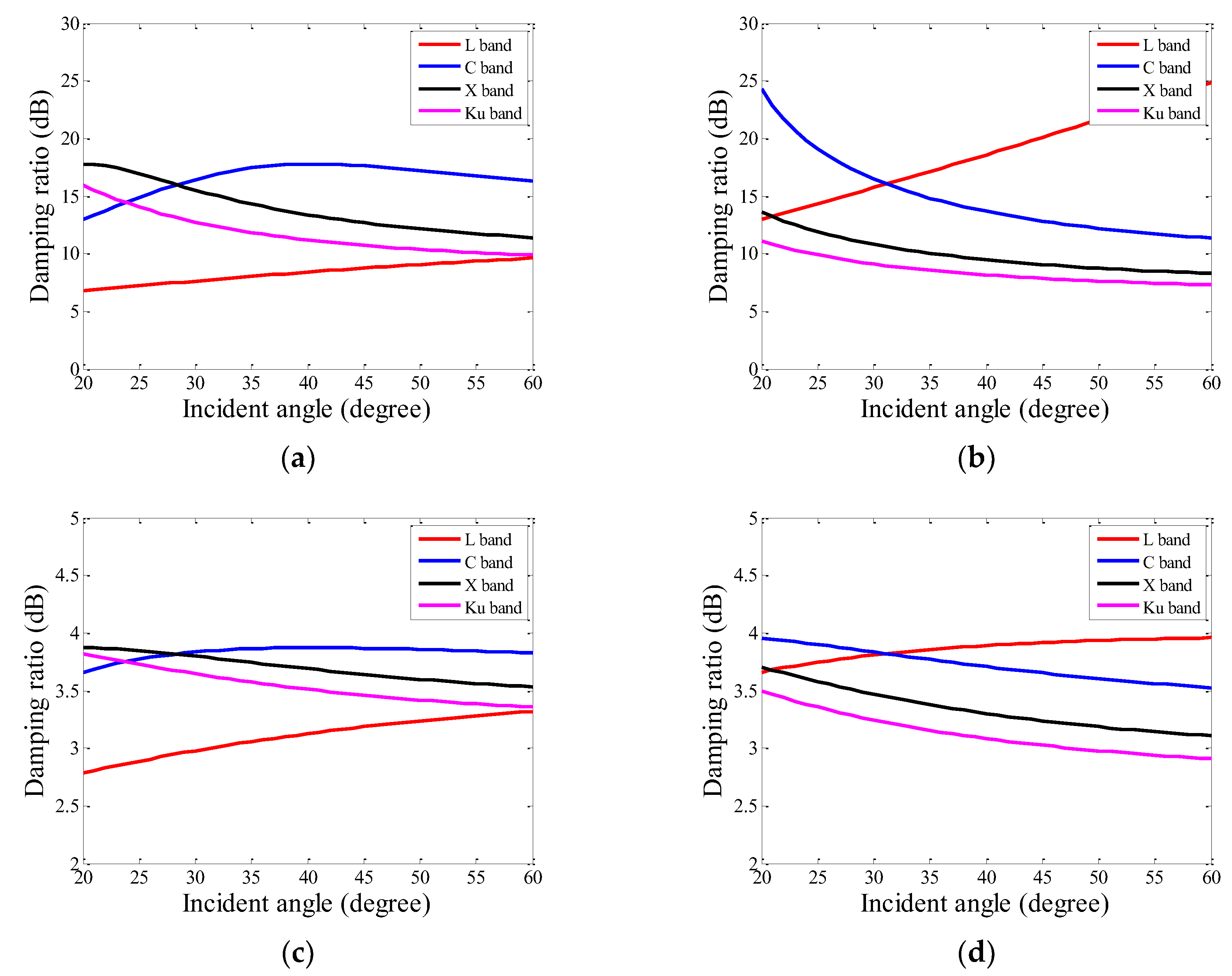
Figure 2 shows the Bragg wavenumber ranges corresponding to L-band, C-band, X-band, and Ku-band electromagnetic waves, respectively. The damping ratios that correspond to
F = 1 and
F = 0.6 of two kinds of slicks for four bands are plotted as functions of the incident angles in
Figure 2. In
Figure 2a,c, it can be noted that the damping ratios for the X-band and Ku-band monotonically decrease with incident angle. While for the C-band, the damping ratio first increases and then decreases. For the L-band, the damping ratio monotonically increases with incident angle. In
Figure 2b,d, it can be noted that the damping ratios for the C-band, X-band, and Ku-band decrease with incident angle. While for the L-band, the damping ratio increases with incident angle. The C-band has a larger damping ratio than the other three bands. Comparing
Figure 2a with
Figure 2c, and
Figure 2b with
Figure 2d,
F makes significant influences on the damping ratios at four bands, which correspond to
Figure 1. According to equations (3) and (8), we know that the Bragg wavenumbers that correspond to different bands are different, and the damping ratios for different Bragg wavenumbers are also different. As a consequence, the damping effects caused by slicks on the L-band, C-band, X-band, and Ku-band are different.
3.1.2. Impacts of Slick on the Curvature Spectrum
A sea spectrum describes the distribution of each harmonic component of the sea surface as functions of the spatial wavenumber and wind direction. Usually, it can be expressed as:
where
represents the omnidirectional part and
represents the spreading function.
is the angle between the observation angle and upwind direction. In the literature, various sea spectral models have been proposed; among these models, the Elfouhaily spectrum is one of the most widely used sea spectra in ocean remote sensing [
24,
25]. In this work, the Elfouhaily spectrum is employed to describe sea waves.
Figure 3 shows the impacts of the Marangoni damping effect (denoted as D), the reduction of friction velocity (denoted as R), and
F on the curvature spectrum
, where
, and
. The wind speed at 10-m height (
U10) is set as 7 m/s. In
Figure 3a, we can note that the short-gravity and capillary waves are damped significantly due to the Marangoni effect. In fact, the Marangoni effect mainly influences the small-scale waves, and it makes no influences on the large-scale waves. Moreover, slick-b has a heavier damping effect than slick-a when
k <100 rad/m, while slick-a has a heavier damping effect when
k >100 rad/m. Besides, the reduction of friction velocity mainly influences the large-scale waves and makes slight influences on the small-scale waves. The reduction of friction velocity is not associated with the properties of slicks. As illustrated in
Figure 3b, the fractional filling factor
F only influences the short-gravity and capillary waves. The differences between the two kinds of slicks become smaller when the value of
F gets smaller.
3.1.3. Impacts of Slick on the RMS Height and the RMS Slope
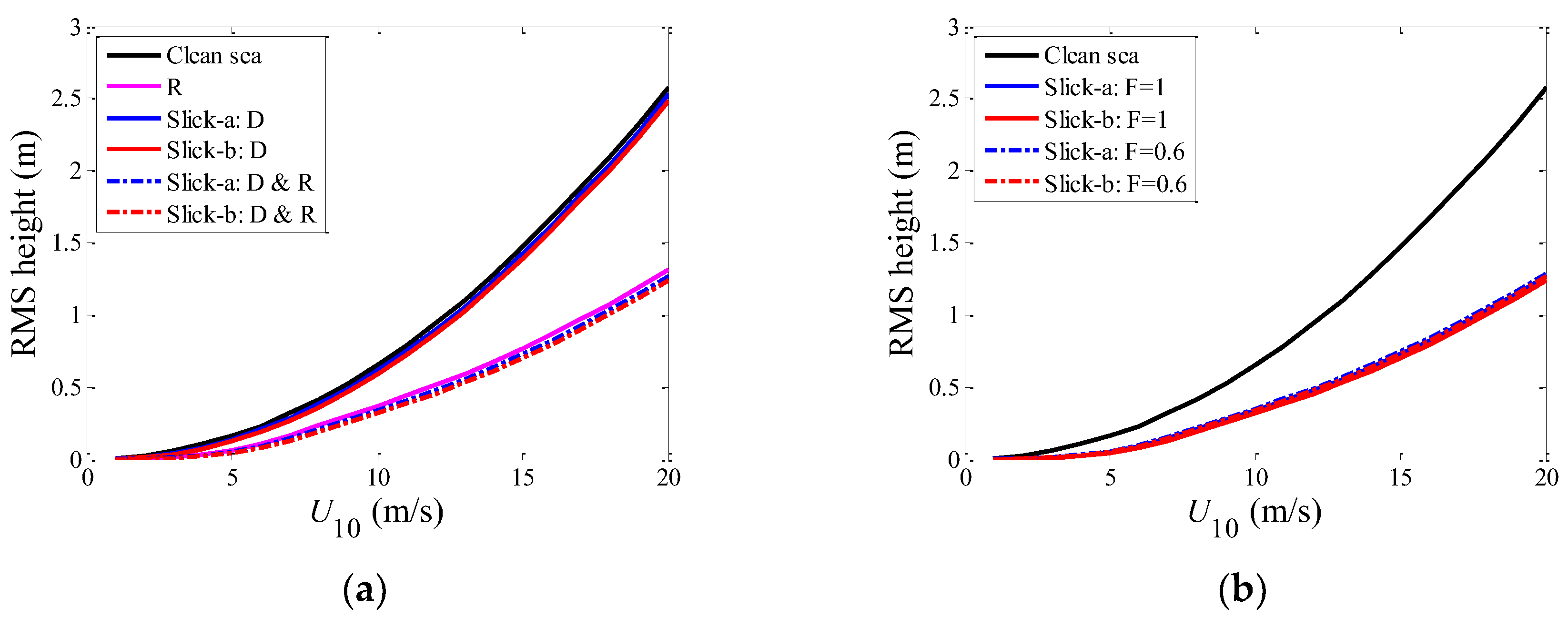
The profile of the sea spectrum changes when an oil slick presents on the sea surface, which results in changes in the slope variances and height variances.
Figure 4 presents the RMS heights of the sea surfaces under different conditions. It can be observed in
Figure 4 that the influences of the Marangoni effect and
F on the RMS height are quite small. In addition, the curves of the two kinds of slicks are similar, and the reduction of friction velocity is the main reason for the reduction of the RMS height.
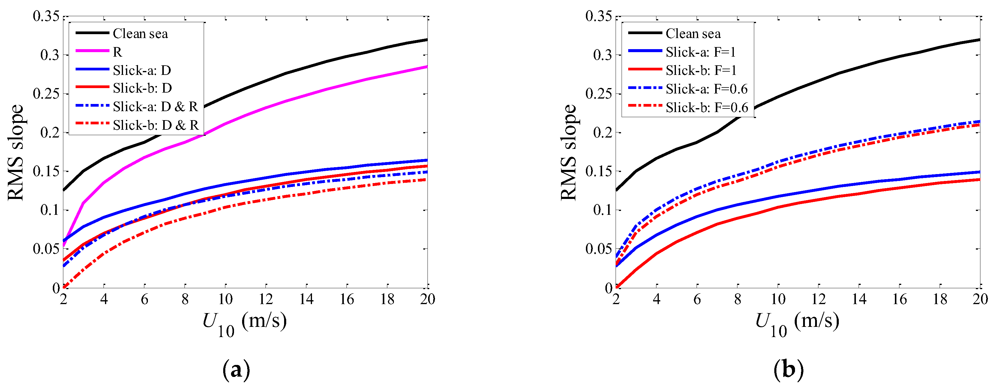
Figure 5 shows the RMS slopes of sea surfaces plotted as functions of wind speed. In fact, the RMS height mainly depends on the large-scale waves, while the RMS slope depends both on the large-scale and the small-scale waves. Thus, unlike the RMS height, the influence of the reduction of the friction velocity on the RMS slope cannot be neglected. The influence caused by the Marangoni effect seems more obvious than the reduction of friction velocity. For
Figure 5b, the value of
F has a significant influence on the RMS slope. The RMS slope is also modulated by the physical property of different kinds of slicks.
3.1.4. Impacts of Slick on the Autocorrelation Function
The autocorrelation of the displacement field of the sea surface profile corresponds to the inverse Fourier transform of the sea spectrum. It describes the correlations between two arbitrary points on the rough surface. In the numerical simulation by the SSA-2, the scattering coefficient is related to the autocorrelation function. As limited by the length of the paper, we cannot provide a detailed discussion here; for more discussions about the autocorrelation function, please refer to Voronovich et al. [
20]. It is interesting to compare the autocorrelation functions of slick-free and slick-covered sea surfaces, since the correlation length and the autocorrelation function shape are also closely related to the roughness of the rough surface.
Figure 6 shows the autocorrelation functions normalized by the height variances of the sea surfaces. In
Figure 6a, the impacts of slicks on the autocorrelation function are similar to the RMS height. The reduction of friction velocity is very influential upon the autocorrelation function. In contrast, the Marangoni effect changes the autocorrelation function slightly. In
Figure 6b, the value of
F also makes negligible influences on the autocorrelation function. Through
Figure 6, it can be noted that the reduction of friction speed makes a shorter correlation length, and the two kinds of slicks produce similar impacts on the shape of autocorrelation functions.
3.2. NRCS of Slick-Free and Slick-Covered Sea Surfaces
In this part, the normalized radar cross-sections (NRCS) of slick-free and slick-covered sea surfaces are estimated according to
Section 2. For slick-free sea surface, the NRCSs simulated by the SSA-2 are compared with those obtained using the geophysical model functions (GMFs), the classic TSM, and the SSA-1, respectively. For slick-covered sea surface, the simulated NRCSs of the SSA-2 are compared with the SAR data acquired by the C-band Radarsat-2 and the L-band uninhabited aerial vehicle synthetic aperture radar (UAVSAR).
3.2.1. NRCS of Slick-Free Sea Surfaces
GMFs are empirical models that are related to the incident angle, wind speed, and wind direction. The GMFs are often applied for wind field retrieval. It has been proven that GMFs could provide accurate predictions in practical applications. Thus, the NRCS estimated with GMFs can be regarded as reliable references. To evaluate the effectiveness of the SSA-2 for sea surface NRCSs estimation, in this part, the NRCSs calculated with the SSA-2 are compared with those obtained from L-band GMF [
26], C-band CMOD7 [
27], C-band CSARMOD [
28], X-band XMOD2 [
29], and Ku-band NSCAT4 [
30], respectively. Besides, the SSA-2 is also compared with the classic TSM and the SSA-1.
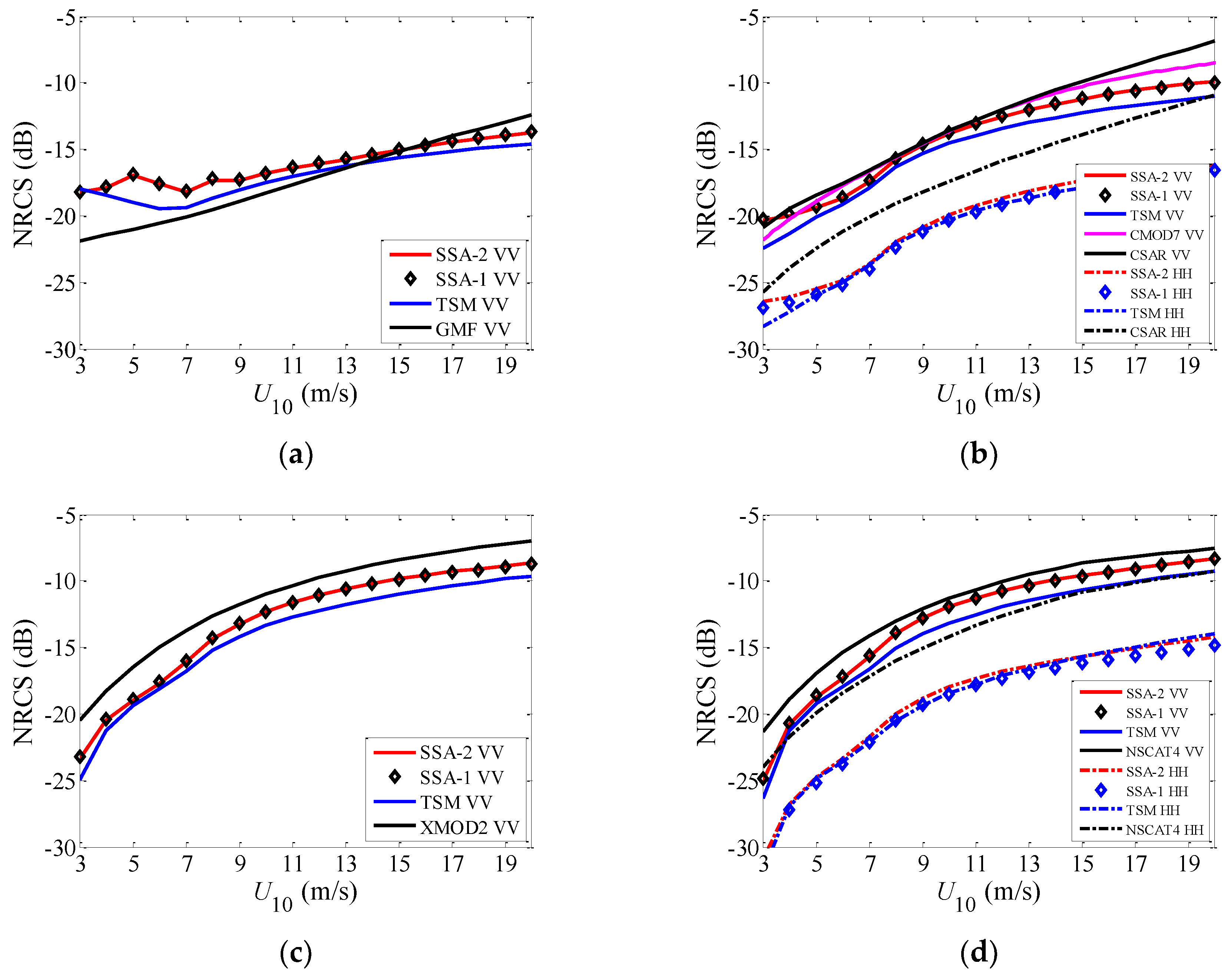
Figure 7 shows the NRCSs computed using the SSA-1, the SSA-2, the TSM, and the GMFs. It should be noted that the L-band GMF can be employed only for HH polarization, the CMOD7 is valid for VV polarization, the CSARMOD is valid for both HH and VV polarizations, the XMOD2 is valid for VV polarization, and the NSCAT4 is valid for both HH and VV polarizations (where ‘V’ denotes the vertical polarization, and ‘H’ denotes the horizontal polarization). Firstly, in
Figure 7, it can be noted that the difference between the SSA-1 and the SSA-2 is quite small both for HH and VV polarization. Compared with TSM, it is quite similar for incident angles larger than 30° for all four bands. While the incident angle is smaller than 30°, there exist larger differences among the C-band, X-band, and Ku-band. With respect to the SSA-2, the scattering coefficient is influenced by surface sample intervals and surface length. The discrepancies between the SSA-2 and TSM for incident angles smaller than 30° at the C-band, X-band, and Ku-band may be introduced by the surface length. For an HV-polarized channel, the curves of the SSA-2 and the TSM are similar to each other. Through
Figure 7a–d, compared with GMFs at different bands, the VV polarized scattering coefficient with the SSA-2 agrees well with the GMFs. While for HH-polarized channels at the C-band and Ku-band, there exist quite larger differences between the SSA-2 and the NSCAT4. That is to say, the SSA-2 simulates VV-polarized NRCS more accurately than HH polarization.
Figure 8 illustrates the NRCSs estimated with different methods under different wind speeds. In
Figure 8, we can note that the NRCSs of the SSA-1 are almost the same with the SSA-2. Combing the results presented in
Figure 7, we can know that the NRCS estimated by the SSA-1 is precise enough in most cases. However, the drawback of the SSA-1 is that it cannot provide the estimation of cross-polarized NRCS in a backscattered direction. In
Figure 8a, for the SSA-2 and the TSM, it is hard to say which method is better. These two methods have similar accuracies, with small overestimation or underestimation of the NRCSs for the small or large wind speed. In
Figure 8b–d, for VV-polarized NRCS estimation, the SSA-2 seems better than the TSM. In fact, the differences between the SSA-2 and the TSM are not large. That is to say, the TSM is also an effective method in EM scattering computations. Meanwhile, the main disadvantage of the TSM is that it involves an arbitrary parameter, i.e., the scale-dividing parameter (
kd, in this paper,
kd =
ki/3) separating the small- and large-scale components of the roughness. With respect to HH-polarized channels at the C-band and Ku-band, the curves of the SSA-2 are quite different from those of the GMFs. Assuming that the GMFs are precise enough, through the comparisons presented in
Figure 8, we can know that the SSA-2 provides better results for a VV-polarized channel than an HH-polarized channel. The SSA-2 performs better than TSM at the C-band, X-band, and Ku-band.
3.2.2. NRCS of Slick-Covered Sea Surfaces at the C-Band
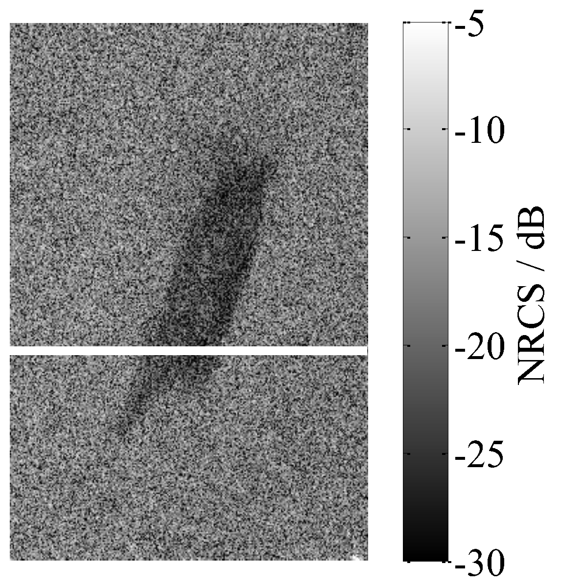
The RADARSAT-2 data acquired at the C-band has been employed to study oil spill on sea surfaces [
31]. The radarsat-2 data used in this part was acquired during the oil spill experiment conducted by the Norway Clean Seas Association for Operating Companies (NOFO) in the North Sea [
32]. The acquisition time is 17:27 (UTC), 8 June 2011. The resolution in the range and azimuth directions are 5.2 m and 7.6 m, respectively. The incident angle is about 34.5~36.1°. The dark area in
Figure 9 is biogenetical slick. The wind speed is 1.6~3.3 m/s.
In
Figure 10, the NRCSs in VV, HH, and HV-polarized channels are presented, respectively. In the numerical simulation, the wind speed
U10 is set as 3.3 m/s. The NRCSs of RADARSAT-2 data are extracted along the white line in
Figure 9. As shown in
Figure 10, for clean sea surface, the VV-polarized and HH-polarized NRCSs of the SSA-2 agree better with the RADARSAT-2 data than HV-polarized channel. For the slick-covered surface, the VV-polarized NRCS estimated with the SSA-2 is consistent with the RADARSAT-2 data when
F = 0.7.
It is well-known that the VV polarization channel is preferred because of its larger radar cross-section from the sea surface, which yields larger differences between the sea surfaces covered with and without oil slicks [
33]. Combining the results exhibited in
Figure 10, we can note that the VV-polarized NRCS with the SSA-2 is more suitable to study the EM scattering than the HH and HV-polarizations.
3.2.3. NRCS of Slick-Covered Sea Surfaces at the L-Band
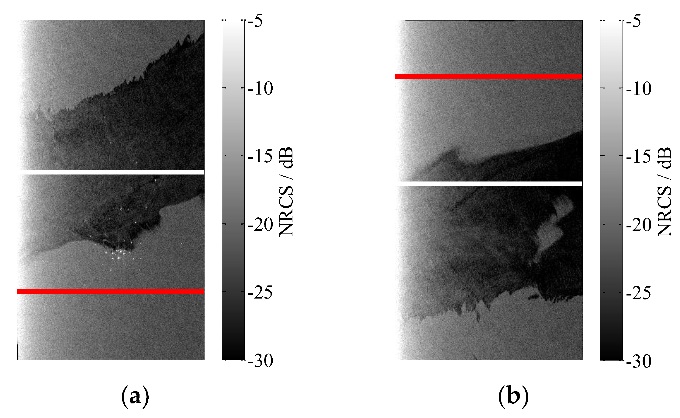
The L-band SAR images used in this part are acquired by uninhabited aerial vehicle synthetic aperture radar (UAVSAR) during the Deepwater Horizon (DWH) oil spill accident in the Gulf of Mexico in 2010 [
34,
35]. UAVSAR is a fully polarimetric L-band SAR. The center frequency of the incident wave is 1.2575 GHz. Two multi-look (three and 12 looks in the range and azimuth directions, respectively) UAVSAR images with a 5-m slant range resolution and 7.2-m azimuth resolution are employed in this part. The SAR images used in this work were acquired from two adjacent, overlapping flight tracks that covered the main oil spills in the Gulf of Mexico. The two flight lines are gulfco_14010_10054_100_100623 (hereafter denoted as Case (a)) and gulfco_32010_10054_101_100623 (hereafter denoted as Case (b)), respectively. More information about the data are summarized in
Table 1 [
33].
The UAVSAR images are presented in
Figure 11, where the dark areas indicate the oil spills. To compare the simulated results with the UAVSAR data, transects related to oil-free (red lines in
Figure 11) as well as oil-covered sea surface (white lines in
Figure 11) are extracted from SAR images and compared with the SSA-2 predictions. In order to compare the simulated results with measured data, the UAVSAR data are processed as follows. Firstly, a 100 × 3300 matrix is obtained by extracting 100 rows of pixels along the red and white lines in
Figure 11. Then, a 1 × 3300 array can be obtained by computing the mean value of each column. Finally, the mean values are calculated in each 1° incident angle range.
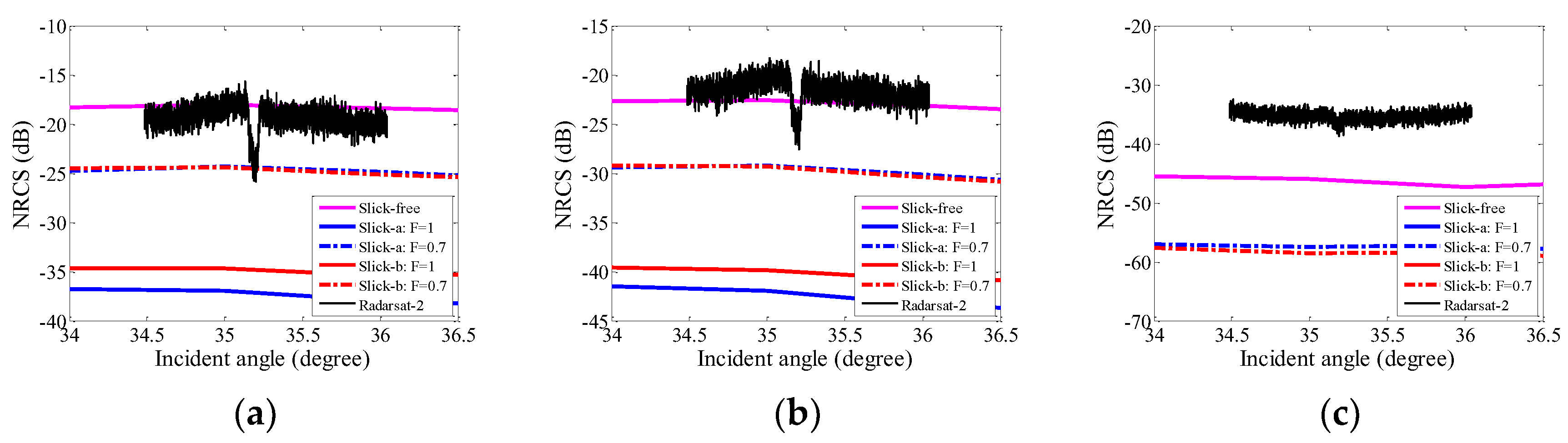
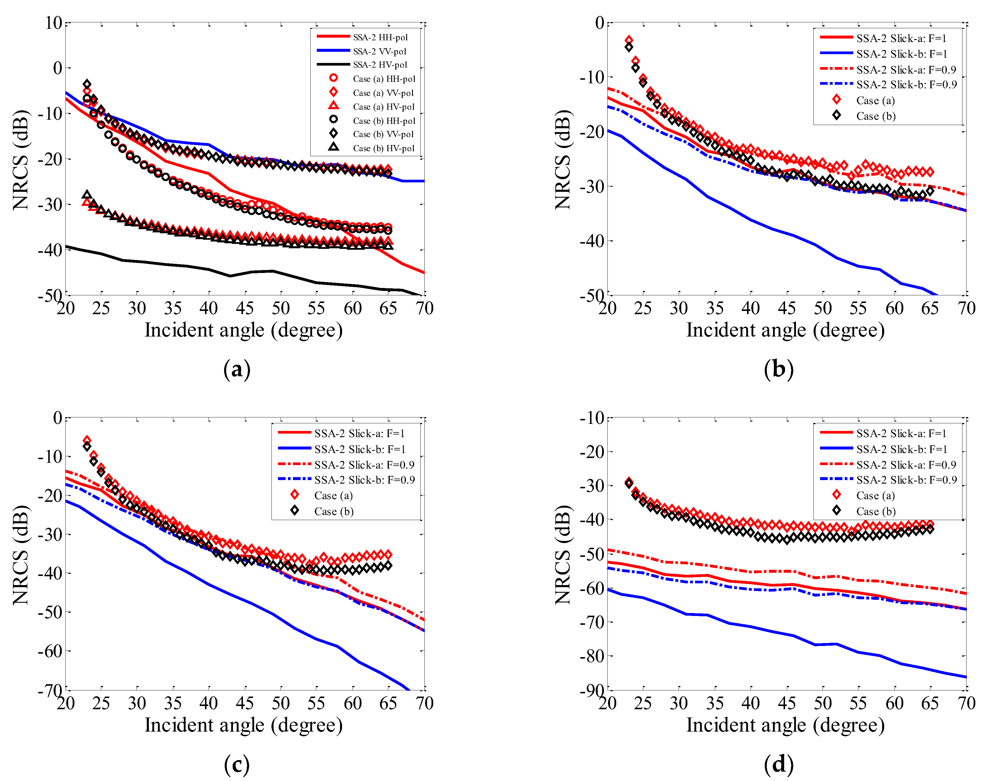
Figure 12 presents the comparisons between the results simulated by the SSA-2 and UAVSAR data for sea surfaces without and with slicks, respectively. In
Figure 12a, for slick-free sea surface, one can see that the VV-polarized NRCS simulated by the SSA-2 agrees well with the measured UAVSAR data. For HH polarization, the SSA-2 cannot provide a prediction as well as VV polarization. This conclusion is similar to the case of TSM presented by Wright et al. [
36]. For the cross-polarized NRCS, the differences between the SSA-2 and UAVSAR are quite large. Additionally, there exist small differences between two UAVSAR images. This may be attributed to the differences of the thickness or the filling proportion between the two images. With respect to sea surface covered with slicks, the NRCSs of slick-covered sea surface with
F = 1 and
F = 0.9 are plotted in
Figure 12b, 12c, and 12d, respectively. In
Figure 12b, the fractional filling factor
F affects slick-b heavier than slick-a. The NRCS extracted from Case (a) agrees well with the results obtained based on slick-a for
F = 1 and slick-b for
F = 0.9. The NRCS extracted from Case (b) agrees well with the results obtained based on slick-a for
F = 0.9. In fact, as the actual values of the physical parameters and the fractional filling factor for the oil spills in
Figure 11 cannot be known, it is hard to compare the numerical results with measured data in detail.
For HH-polarized NRCS, as exhibited in
Figure 12c, the numerical results match well with the UAVSAR data for incident angles from 25° to 55°. In
Figure 12d, there exist large differences between the simulated results and measured data for cross-polarized NRCS.
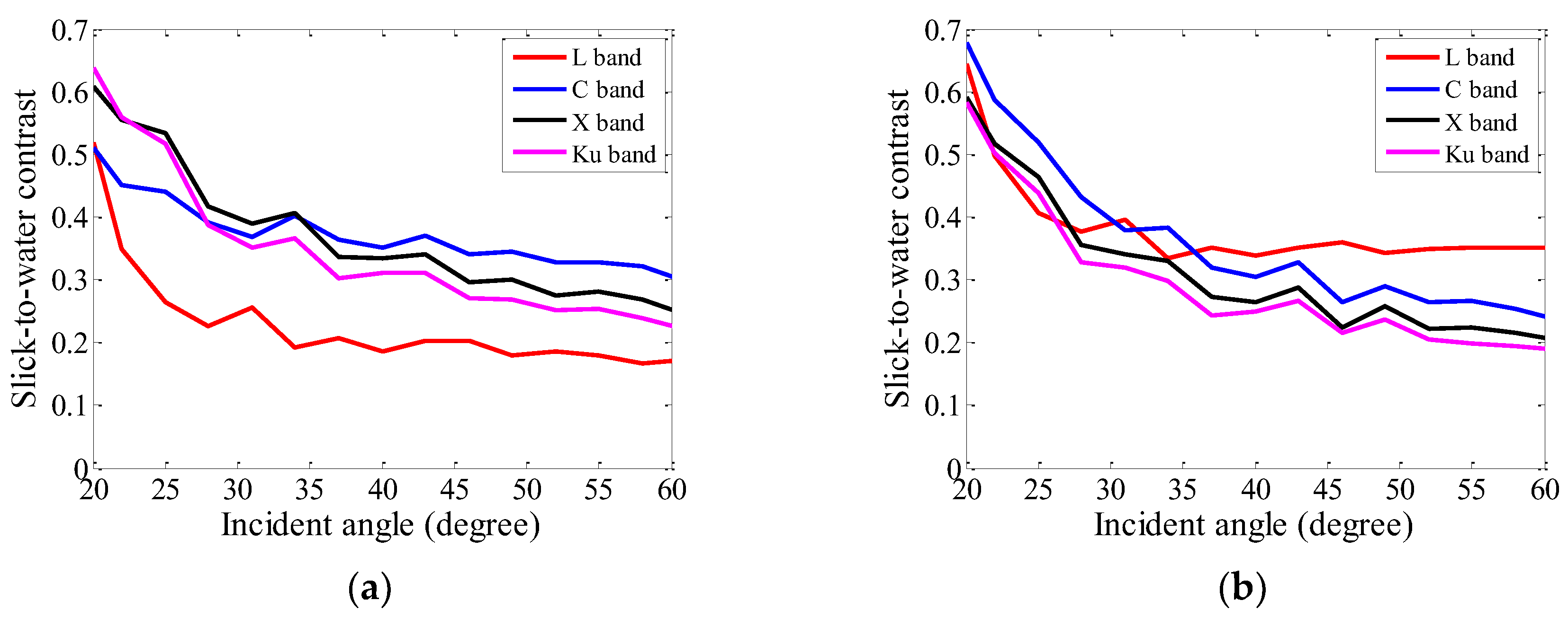
3.3. Distinguishing Ability of Different Bands
In previous sections, both for slick-free and slick-covered sea surfaces, it has shown that the SSA-2 could provide an accurate prediction for VV-polarized NRCS. In order to study the capacities of different bands for oil distinguish further, the slick-to-water contrasts at different bands are studied based on VV polarization. A slick-to-water contrast can be defined as [
11]:
where
is the NRCS of the slick-covered sea surface, and
is the NRCS of the slick-free sea surface. A larger value of
C indicates that slick makes a more significant influence on NRCS. As a consequence, it can be more easily separated from sea backgrounds. Thus, the slick-to-water contrast can be taken as a measurement of distinguishability for different bands to separate slicks from sea backgrounds.
Figure 13 shows the slick-to-water contrasts evaluated with the SSA-2 as functions of incident angles. A common scatterometer typically operates at a moderate incident angle between about 20–60°. Thus, the incident angle is limited from 20° to 60°. Both for slick-a and slick-b, it seems that the value of C is larger for the smaller incident angle. The distinguishing abilities of four bands change with incident angle. For slick-a, it seems that the X-band has a larger C-value than other three bands for incident angles smaller than about 35°. For incident angles between 35–60°, the C-band is preferred to distinguish slick-a. For slick-b, it seems that the C-band has a larger
C-value than the other three bands for incident angles smaller than about 35°. For incident angles between 35–60°, the L-band performs better than the other three bands.
4. Conclusions and Perspectives
In this paper, the EM backscattering from slick-free and slick-covered sea surfaces are investigated by the SSA-2 and measured SAR data. The slick-covered sea surface has been compared with the slick-free sea surface from several aspects, including the sea curvature spectrum, the RMS height, the RMS slope, and the autocorrelation function. According to the numerical simulations, we find that:
(1) The reduction of friction velocity mainly influences the large-scale waves and makes a slight influence on the small-scale waves. Meanwhile, the Marangoni effect mainly influences the small-scale waves.
(2) The influences of the Marangoni effect and F on the RMS height and the autocorrelation function are quite small. The reduction of friction velocity is the main reason for the changes of the RMS height and the autocorrelation function.
(3) By comparing the numerical results of the SSA-2 with GMFs, we can know that the SSA-2 provides accurate predictions for VV-polarized NRCS. Compared with the classic TSM, the SSA-1, the SSA-2 has more advantages in EM scattering simulations.
(4) By comparing the numerical results of the SSA-2 with measured SAR data, we can know that the SSA-2 provides accurate predictions for VV-polarized NRCS. The simulated VV polarized NRCS of the SSA-2 can be used to study the EM scattering from both slick-free and slick-covered sea surfaces.
(5) The distinguishing abilities (which are associated with the defined parameter ‘slick-to-water contrast’) of microwave scatterometers at various bands are different for different kinds of slicks and incident angles.
This work provides a basic study for EM scattering from slick-free and slick-covered sea surfaces. However, the comparisons between numerical simulations and measured data are only conducted at the C-band and L- band. In further works, more experiments and investigations will be carried out based on measured SAR data for other bands, especially the X-band and Ku-band.
Author Contributions
H.Z., Y.Z., and A.K. contributed the main idea. H.Z. performed the simulations and wrote the manuscript. H.G. contributed to the CMOD7 and modified the manuscript. Y.W. and C.Z. modified the manuscript.
Funding
This work is supported by the National Key Research and Development Program of China (2016YFC1401007), the National Natural Science Foundation of China (41576170, 41376179), and the scholarship from China Scholarship Council (201706330021).
Acknowledgments
The authors would like to thank the NASA/JPL for providing UAVSAR data used in this paper.
Conflicts of Interest
The authors declare no conflict of interest.
Appendix A
Appendix A.1. Monte-Carlo Method for Sea Surface Profile Simulation
The sea surface profile, which could provide some insights on the SAR imaging mechanism, is essential for the SSA-2 numerical simulation [
37]. Assuming the side lengths of the simulated sea are (
Lx,
Ly). The sampling numbers in
x and
y directions are
M and
N. Therefore,
Lx =
MdLx and
Ly =
NdLy, where
dLx and
dLy are the distances between two adjacent points in
x and
y directions. The sea surface height at
r = (
x,
y) (
x = mk·dLx,
y = nk·dLy, where
mk = −
M/2 + 1, …,
M/2,
nk = −
N/2 + 1, …,
N/2) can be simulated with:
where
S(
kx,
ky) is the two dimensions sea surface height spectrum.
kx =
mdkx and
ky =
ndky, where
dkx = 2
π/
Lx and
dky = 2
π/
Ly.
R(0, 1) is a Gaussian series with zero mean and unity standard deviation. To make the sea surface height
h(
x,
y) is real,
T(
km,
kn) should satisfy
T(
km,
kn) =
T * (−
km, −
kn),
T(
km, −
kn) =
T * (−
km,
kn), where ‘*’ denotes conjugate. In the numerical simulation, Equation (A2) is realized by using the inverse Fourier transform.
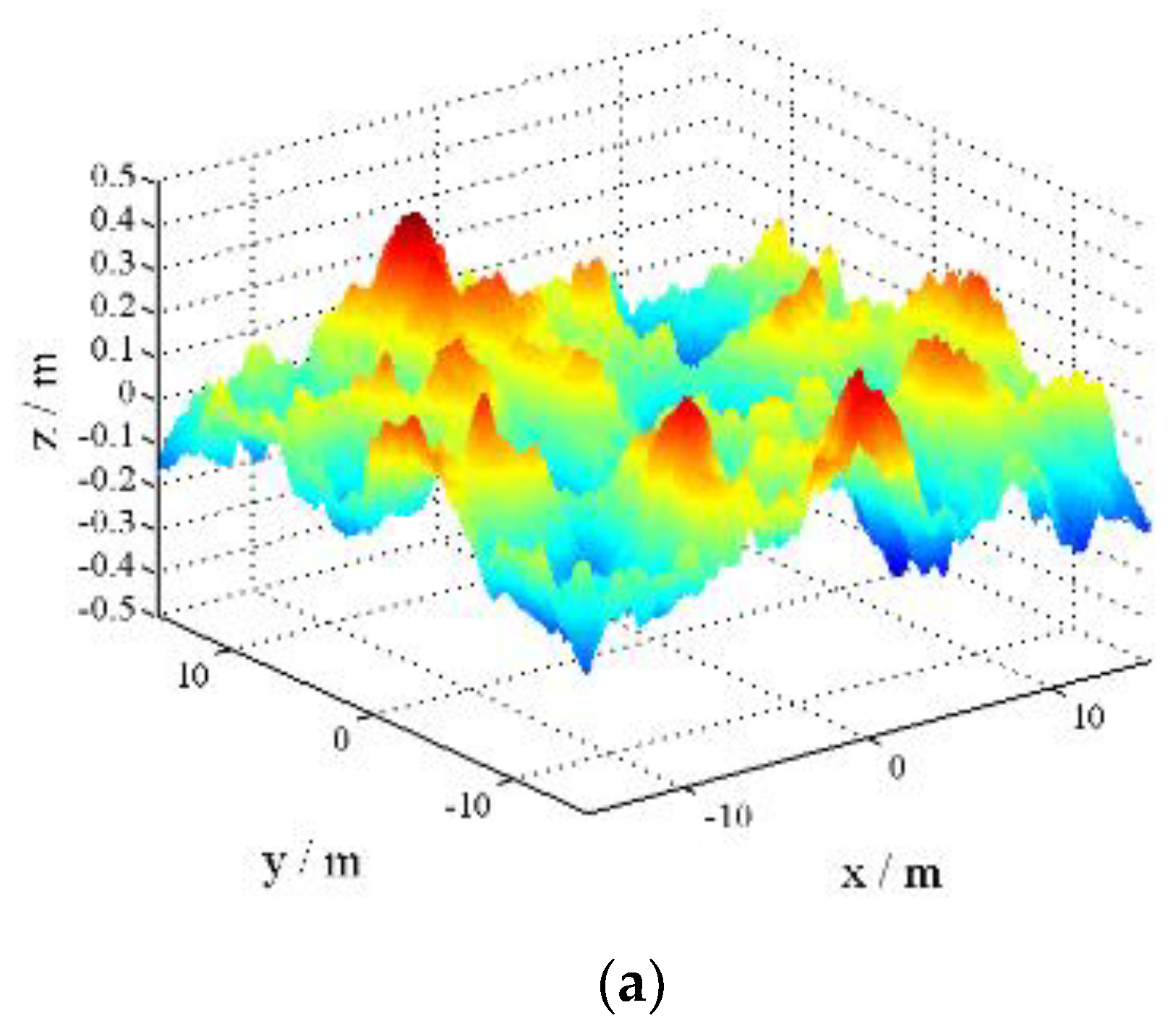
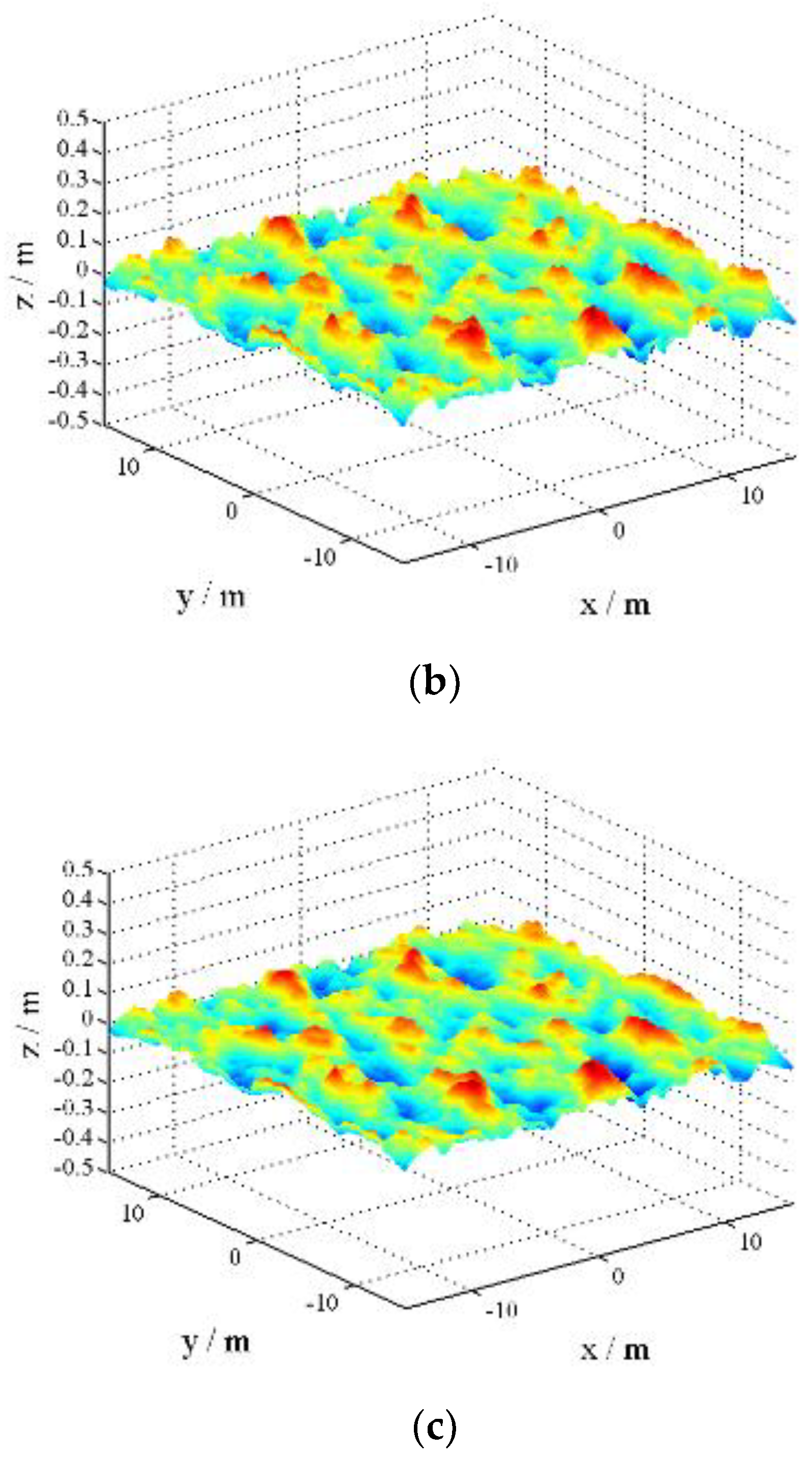
Figure A1 presents the generated two-dimension sea surfaces height without and with slicks. In this paper, there are 1024 sampling points at
x and
y directions, respectively. The sampling interval is
λi/8, where
λi is the wavelength of the incident wave. In
Figure A1,
λi is set as 0.2386 m which corresponds to L band. It can be easily seen that the large-scale waves of slick-covered sea surfaces are reduced due to the reduction of friction velocity.
Figure A1.
Sea surface height, U10 = 5 m/s. (a) Clean sea. (b) With slick-a. (c) With slick-b.
Figure A1.
Sea surface height, U10 = 5 m/s. (a) Clean sea. (b) With slick-a. (c) With slick-b.
Appendix A.2. The Second Order Small Slope Approximation
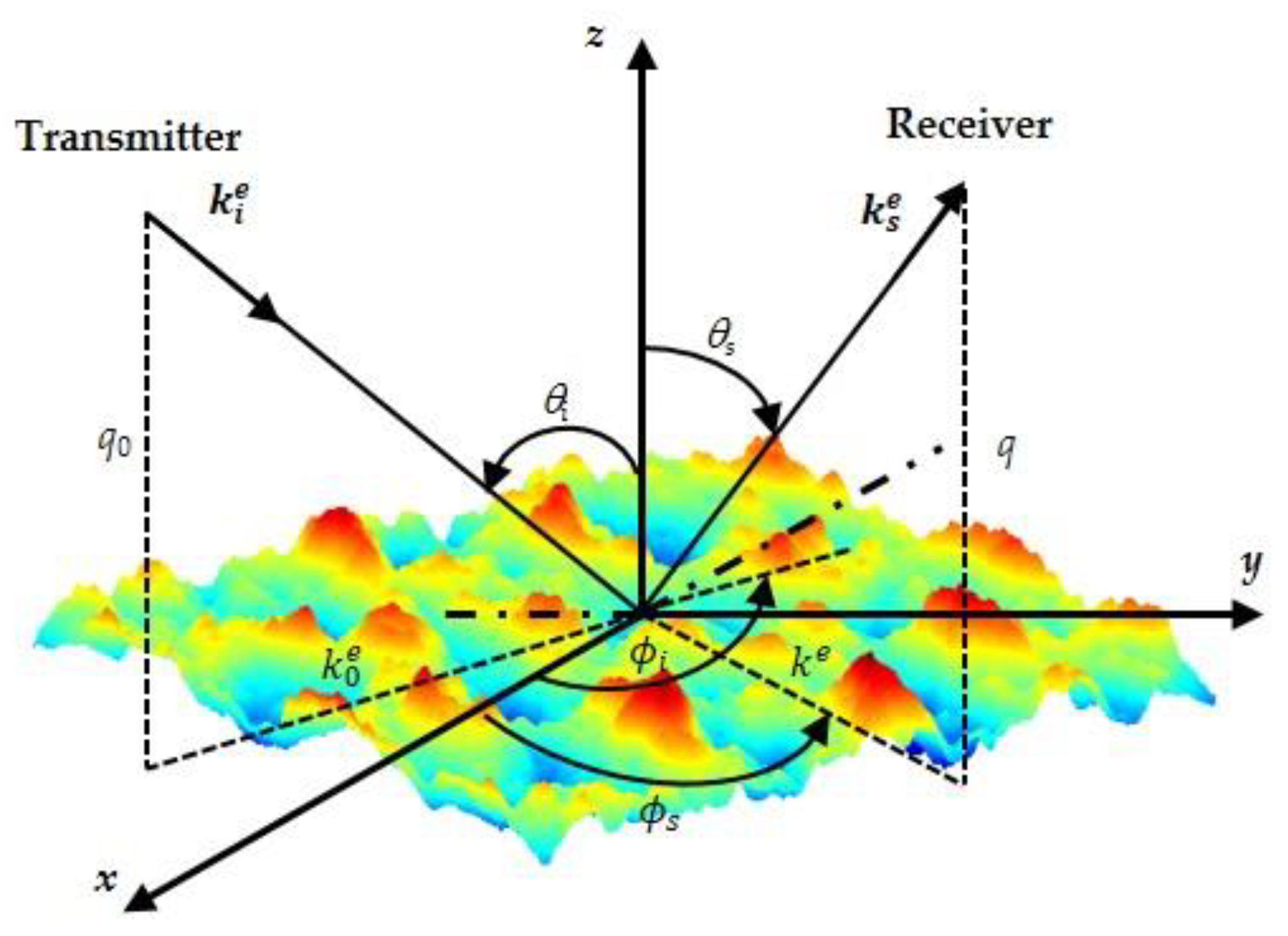
The EM scattering configuration is plotted in
Figure A2. Assuming the EM wave incidents on the two-dimension sea surface
z =
h(
r). The two-dimension sea surface height can be generated with the Monte-Carlo model. The incident wave vector denoted as
and the scattering wave vector denoted as
.
θi,
φi,
θs,
φs denote the incident angle, incident azimuth angle, scattering angle and scattering azimuth angle, respectively.
Figure A2.
Configuration of EM scattering from sea surface.
Figure A2.
Configuration of EM scattering from sea surface.
The unit vector in the directions of incidence and scattering are:
and
can be decomposed into horizontal and vertical components:
where
,
,
and
.
In the numerical simulations, the length of the simulated sea is finite, which leads to that the surface electric/magnetic current is forced to be zero at the boundary. If there is an abrupt change of surface electric/magnetic current from nonzero to zero, the effect of truncation would be very significant. To solve this problem, a tapered incident wave is used to make that the incident wave decays to zero in a Gaussian manner near the boundary [
38].
The incident field can be written as:
where
wave
, and
g is the parameter that controls the tapering of the incident wave. In general, the value of g is between
L/4 to
L/10, depending on the incident angle. Here,
g is set as
L/6. Moreover, it should be pointed out that, the taper function is not suited for problems of low grazing angle, i.e.,
θi→90°.
The scattered field can be expressed as:
In the case of far-field scattering, the scattering amplitude corresponding to the second-order SSA can be calculated with [
19]:
where
B and
B2 are kernel functions which have been given in [
19,
20].
is the Fourier transform of the sea surface height.
Pinc is the incident wave power illuminated on the rough surface and can be expressed as:
The scattering coefficient can be calculated with scattering amplitude by:
where
denotes the ensemble average operator. In this work, each NRCS is obtained over 80 realizations of sea surfaces. Limited by the length of the paper, parts of derivations of the SSA-2 are omitted here. For more details about the SSA-2, please see ref. [
19,
20].
References
- Salberg, A.B.; Rudjord, Ø.; Solberg, A.H.S. Oil spill detection in hybrid-polarimetric SAR images. IEEE Trans. Geosci. Remote Sens. 2014, 52, 6521–6533. [Google Scholar] [CrossRef]
- Skrunes, S.; Brekke, C.; Eltoft, T.; Kudryavtsev, V. Comparing Near-Coincident C- and X-Band SAR Acquisitions of Marine Oil Spills. IEEE Trans. Geosci. Remote Sens. 2015, 53, 1958–1975. [Google Scholar] [CrossRef]
- Lupidi, A.; Staglianò, D.; Martorella, M.; Berizzi, F. Fast detection of oil spills and ships using SAR images. Remote Sens. 2017, 9, 230. [Google Scholar] [CrossRef]
- Gleason, S.; Ruf, C.S.; Clarizia, M.P.; O’Brien, A.J. Calibration and Unwrapping of the Normalized Scattering Cross Section for the Cyclone Global Navigation Satellite System. IEEE Trans. Geosci. Remote Sens. 2016, 54, 2495–2509. [Google Scholar] [CrossRef]
- Migliaccio, M.; Nunziata, F.; Buono, A. SAR polarimetry for sea oil slick observation. Int. J. Remote Sens. 2015, 36, 3243–3273. [Google Scholar] [CrossRef] [Green Version]
- Solberg, A.H.S.; Brekke, C.; Ove Husoy, P. Oil spill detection in Radarsat and Envisat SAR images. IEEE Trans. Geosci. Remote Sens. 2007, 45, 746–755. [Google Scholar] [CrossRef]
- Buono, A.; Nunziata, F.; Migliaccio, M.; Li, X. Polarimetric analysis of compact-polarimetry SAR architectures for sea oil slick observation. IEEE Trans. Geosci. Remote Sens. 2016, 54, 5862–5874. [Google Scholar] [CrossRef]
- Migliaccio, M.; Nunziata, F.; Gambardella, A. On the co-polarized phase difference for oil spill observation. Int. J. Remote Sens. 2009, 30, 1587–1602. [Google Scholar] [CrossRef]
- Migliaccio, M.; Gambardella, A.; Nunziata, F.; Shimada, M.; Isoguchi, O. The PALSAR polarimetric mode for sea oil slick observation. IEEE Trans. Geosci. Remote Sens. 2009, 47, 4032–4041. [Google Scholar] [CrossRef]
- Migliaccio, M.; Nunziata, F. On the exploitation of polarimetric SAR data to map damping properties of the Deepwater Horizon oil spill. Int. J. Remote Sens. 2014, 35, 3499–3519. [Google Scholar] [CrossRef]
- Zheng, H.; Zhang, Y.; Wang, Y.; Zhang, X.; Meng, J. The polarimetric features of oil spills in full polarimetric synthetic aperture radar images. Acta Oceanol. Sin. 2017, 36, 105–114. [Google Scholar] [CrossRef]
- Ghanmi, H.; Khenchaf, A.; Comblet, F. Bistatic electromagnetic scattering and detection of pollutant on a sea surface. J. Appl. Remote Sens. 2015, 9, 096007. [Google Scholar] [CrossRef]
- Pinel, N.; Déchamps, N.; Bourlier, C. Modeling of the bistatic electromagnetic scattering from sea surfaces covered in oil for microwave applications. IEEE Trans. Geosci. Remote Sens. 2008, 46, 385–392. [Google Scholar] [CrossRef]
- Ghanmi, H.; Khenchaf, A.; Comblet, F. Numerical Modeling of Electromagnetic Scattering from Sea Surface Covered by Oil. J. Electromagn. Anal. Appl. 2014, 6, 15–24. [Google Scholar] [CrossRef]
- Nunziata, F.; Sobieski, P.; Migliaccio, M. The two-scale BPM scattering model for sea biogenic slicks contrast. IEEE Trans. Geosci. Remote Sens. 2009, 47, 1949–1956. [Google Scholar] [CrossRef]
- Alpers, W.; Hühnerfuss, H. The damping of ocean waves by surface films: A new look at an old problem. J. Geophys. Res. Oceans 1989, 94, 6251–6265. [Google Scholar] [CrossRef]
- Rice, S.O. Reflection of electromagnetic waves from slightly rough surfaces. Commun. Pure Appl. Math. 1951, 4, 351–378. [Google Scholar] [CrossRef]
- Ogilvy, J.A.; Merklinger, H.M. Theory of wave scattering from random rough surfaces. J. Acoust. Soc. Am. 1991, 90, 3382. [Google Scholar] [CrossRef]
- Voronovich, A. Small-slope approximation for electromagnetic wave scattering at a rough interface of two dielectric half-spaces. Wave Random Media 1994, 4, 337–367. [Google Scholar] [CrossRef]
- Voronovich, A.; Zavorotny, V. Theoretical model for scattering of radar signals in K u-and C-bands from a rough sea surface with breaking waves. Wave Random Media 2001, 11, 247–269. [Google Scholar] [CrossRef]
- Kim, D.-J.; Moon, W.M.; Kim, Y.-S. Application of TerraSAR-X data for emergent oil-spill monitoring. IEEE Trans. Geosci. Remote Sens. 2010, 48, 852–863. [Google Scholar] [CrossRef]
- Montuori, A.; Nunziata, F.; Migliaccio, M.; Sobieski, P. X-band two-scale sea surface scattering model to predict the contrast due to an oil slick. IEEE J. Sel. Top. Appl. Earth Obs. Remote Sens. 2016, 9, 4970–4978. [Google Scholar] [CrossRef]
- Gade, M.; Alpers, W.; Hühnerfuss, H.; Wismann, V.R.; Lange, P.A. On the reduction of the radar backscatter by oceanic surface films: Scatterometer measurements and their theoretical interpretation. Remote Sens. Environ. 1998, 66, 52–70. [Google Scholar] [CrossRef]
- Elfouhaily, T.; Chapron, B.; Katsaros, K.; Vandemark, D. A unified directional spectrum for long and short wind-driven waves. J. Geophys. Res. Oceans 1997, 102, 15781–15796. [Google Scholar] [CrossRef] [Green Version]
- Zheng, H.; Khenchaf, A.; Wang, Y.; Ghanmi, H.; Zhang, Y.; Zhao, C. Sea Surface Monostatic and Bistatic EM Scattering Using SSA-1 and UAVSAR Data: Numerical Evaluation and Comparison Using Different Sea Spectra. Remote Sens. 2018, 10, 1084. [Google Scholar] [CrossRef]
- Isoguchi, O.; Shimada, M. An L-band ocean geophysical model function derived from PALSAR. IEEE Trans. Geosci. Remote Sens. 2009, 47, 1925–1936. [Google Scholar] [CrossRef]
- Stoffelen, A.; Verspeek, J.A.; Vogelzang, J.; Verhoef, A. The CMOD7 geophysical model function for ASCAT and ERS wind retrievals. IEEE J. Sel. Top. Appl. Earth Obs. Remote Sens. 2017, 10, 2123–2134. [Google Scholar] [CrossRef]
- Mouche, A.; Chapron, B. Global C-Band Envisat, RADARSAT-2 and Sentinel-1 SAR measurements in copolarization and cross-polarization. J. Geophys. Res. Oceans 2015, 120, 7195–7207. [Google Scholar] [CrossRef]
- Li, X.-M.; Lehner, S. Algorithm for sea surface wind retrieval from TerraSAR-X and TanDEM-X data. IEEE Trans. Geosci. Remote Sens. 2014, 52, 2928–2939. [Google Scholar] [CrossRef]
- Wentz, F.J.; Smith, D.K. A model function for the ocean-normalized radar cross section at 14 GHz derived from NSCAT observations. J. Geophys. Res. Oceans 1999, 104, 11499–11514. [Google Scholar] [CrossRef] [Green Version]
- Zhang, B.; Perrie, W.; Li, X.; Pichel, W.G. Mapping sea surface oil slicks using RADARSAT-2 quad-polarization SAR image. Geophys. Res. Lett. 2011, 38, L10602–L10606. [Google Scholar] [CrossRef]
- Skrunes, S.; Brekke, C.; Eltoft, T. Characterization of marine surface slicks by Radarsat-2 multipolarization features. IEEE Trans. Geosci. Remote Sens. 2014, 52, 5302–5319. [Google Scholar] [CrossRef]
- Li, H.; Perrie, W.; He, Y.; Wu, J.; Luo, X. Analysis of the polarimetric SAR scattering properties of oil-covered waters. IEEE J. Sel. Top. Appl. Earth Obs. Remote Sens. 2015, 8, 3751–3759. [Google Scholar] [CrossRef]
- Liu, P.; Li, X.; Qu, J.J.; Wang, W.; Zhao, C.; Pichel, W. Oil spill detection with fully polarimetric UAVSAR data. Mar. Pollut. Bull. 2011, 62, 2611–2618. [Google Scholar] [CrossRef] [PubMed]
- Carratelli, E.P.; Dentale, F.; Reale, F. On the effects of wave-induced drift and dispersion in the Deepwater Horizon oil spill. Monitoring and Modeling the Deepwater Horizon Oil Spill: A Record-Breaking Enterprise. Geophys. Monogr. Ser. 2011, 195, 197–204. [Google Scholar] [CrossRef]
- Wright, J. A new model for sea clutter. IEEE Trans. Antennas Propag. 1968, 16, 217–223. [Google Scholar] [CrossRef]
- Carratelli, E.P.; Dentale, F.; Reale, F. Numerical pseudo-random simulation of SAR sea and wind response. In Proceedings of the SEASAR, Frascati, Italy, 23–26 January 2006; pp. 1–5. [Google Scholar]
- Tsang, L.; Kong, J.A.; Ding, K.-H.; Ao, C.O. Chapter 4 Random rough surface simulations. In Scattering of Electromagnetic Waves: Numerical Simulations; John Wiley & Sons: Hoboken, NJ, USA, 2004; pp. 111–176. ISBN 0-471-38800-9. [Google Scholar]
Figure 1.
The damping ratios of different slicks and fractional filling factors (F).
Figure 1.
The damping ratios of different slicks and fractional filling factors (F).
Figure 2.
The damping ratios in relation with the incident angle. (a) Slick-a, F = 1. (b) Slick-b, F = 1. (c) Slick-a, F = 0.6. (d) Slick-b, F = 0.6.
Figure 2.
The damping ratios in relation with the incident angle. (a) Slick-a, F = 1. (b) Slick-b, F = 1. (c) Slick-a, F = 0.6. (d) Slick-b, F = 0.6.
Figure 3.
The curvature spectra, U10 = 7 m/s. (a) Influenced by the Marangoni effect and reduction of friction velocity, F = 1. (b) Influenced by F with D and R.
Figure 3.
The curvature spectra, U10 = 7 m/s. (a) Influenced by the Marangoni effect and reduction of friction velocity, F = 1. (b) Influenced by F with D and R.
Figure 4.
The RMS heights, U10 = 7 m/s. (a) Influenced by the Marangoni effect and the reduction of friction velocity, F = 1. (b) Influenced by F with D and R.
Figure 4.
The RMS heights, U10 = 7 m/s. (a) Influenced by the Marangoni effect and the reduction of friction velocity, F = 1. (b) Influenced by F with D and R.
Figure 5.
The root mean square (RMS) slopes of sea surfaces, U10 = 7 m/s. (a) Influenced by the Marangoni effect and reduction of friction velocity. (b) Influenced by F with D and R.
Figure 5.
The root mean square (RMS) slopes of sea surfaces, U10 = 7 m/s. (a) Influenced by the Marangoni effect and reduction of friction velocity. (b) Influenced by F with D and R.
Figure 6.
The autocorrelation functions, U10 = 7 m/s. (a) Influenced by the Marangoni effect and reduction of friction velocity. (b) Influenced by F with D and R.
Figure 6.
The autocorrelation functions, U10 = 7 m/s. (a) Influenced by the Marangoni effect and reduction of friction velocity. (b) Influenced by F with D and R.
Figure 7.
The second-order small slope approximation (SSA-2) compared with other models, including the first-order small slope approximation (SSA-1), two-scale model (TSM), and geophysical model functions (GMFs). In relation to the incident angle, U10 = 7 m/s. (a) L-band, (b) C-band, (c) X-band, and (d) Ku-band.
Figure 8.
The SSA-2 compared with other models (SSA-1, TSM, and GMFs). In relation with wind speed, θi = 40°. (a) L-band, (b) C-band, (c) X-band, and (d) Ku-band.
Figure 8.
The SSA-2 compared with other models (SSA-1, TSM, and GMFs). In relation with wind speed, θi = 40°. (a) L-band, (b) C-band, (c) X-band, and (d) Ku-band.
Figure 9.
The RADARSAT-2 image related with slick.
Figure 9.
The RADARSAT-2 image related with slick.
Figure 10.
Comparison between simulated results with RADARSAT-2. (a) VV polarization. (b) HH polarization. (c) HV polarization.
Figure 10.
Comparison between simulated results with RADARSAT-2. (a) VV polarization. (b) HH polarization. (c) HV polarization.
Figure 11.
UAVSAR data. (a) Case (a). (b) Case (b).
Figure 11.
UAVSAR data. (a) Case (a). (b) Case (b).
Figure 12.
Comparison between the estimations of the SSA-2 and UAVSAR data. (a) Slick-free sea surface. (b) Slick-covered sea surface for VV polarization. (c) Slick-covered sea surface for HH polarization. (d) Slick-covered sea surface for HV polarization.
Figure 12.
Comparison between the estimations of the SSA-2 and UAVSAR data. (a) Slick-free sea surface. (b) Slick-covered sea surface for VV polarization. (c) Slick-covered sea surface for HH polarization. (d) Slick-covered sea surface for HV polarization.
Figure 13.
Slick-to-water contrast evaluated with the SSA-2 at different bands in relation to the incident angle, U10 = 7 m/s. (a) Slick-a. (b) Slick-b.
Figure 13.
Slick-to-water contrast evaluated with the SSA-2 at different bands in relation to the incident angle, U10 = 7 m/s. (a) Slick-a. (b) Slick-b.
Table 1.
Uninhabited aerial vehicle synthetic aperture radar (UAVSAR) data information.
Table 1.
Uninhabited aerial vehicle synthetic aperture radar (UAVSAR) data information.
| Case | Data ID | Time of Acquisition | Incident Angle (°) | Wind Speed U10 (m/s) | Wind Direction (°) |
|---|
| (a) | 14010 | 20:42 UTC 23 June 2010 | 22–65 | 2.5–5 | 115–126 |
| (b) | 32010 | 21:08 UTC 23 June 2010 | 22–65 | 2.5–5 | 115–126 |
© 2018 by the authors. Licensee MDPI, Basel, Switzerland. This article is an open access article distributed under the terms and conditions of the Creative Commons Attribution (CC BY) license (http://creativecommons.org/licenses/by/4.0/).

 ,
, 


