Burned-Area Detection in Amazonian Environments Using Standardized Time Series Per Pixel in MODIS Data


 ,
,  and
and
Abstract
:
1. Introduction
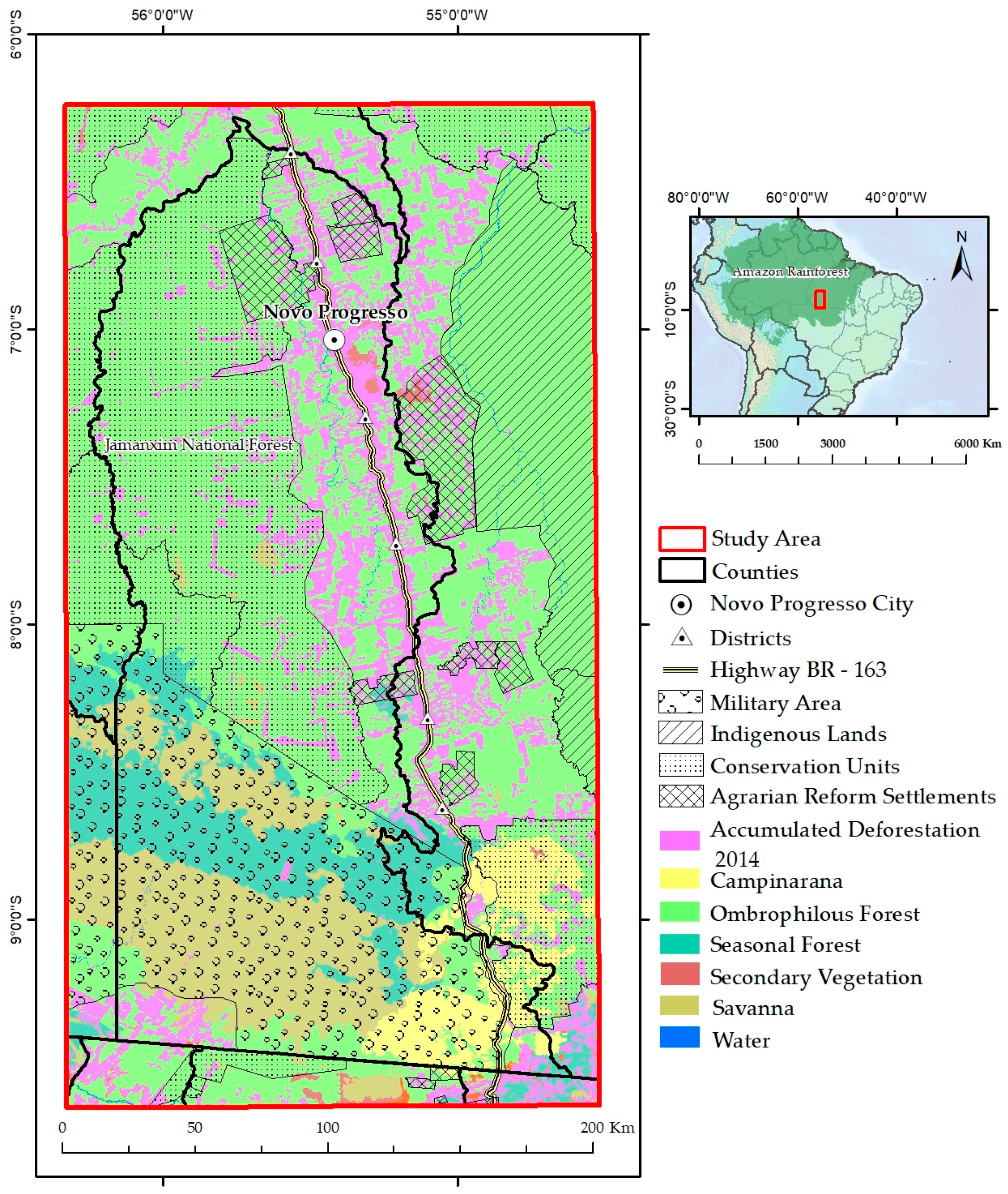
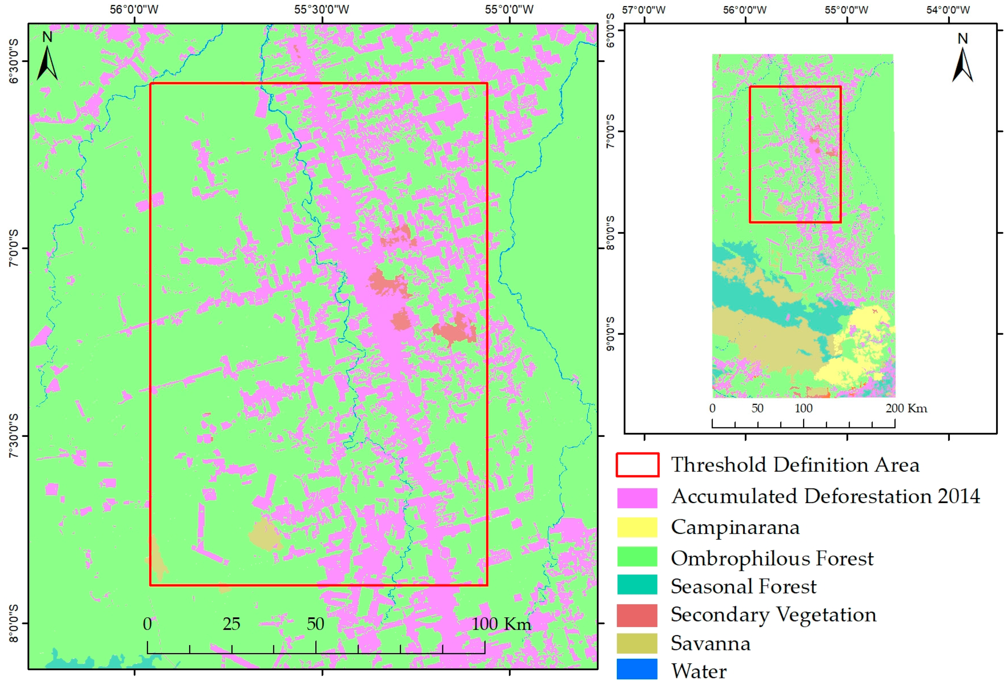
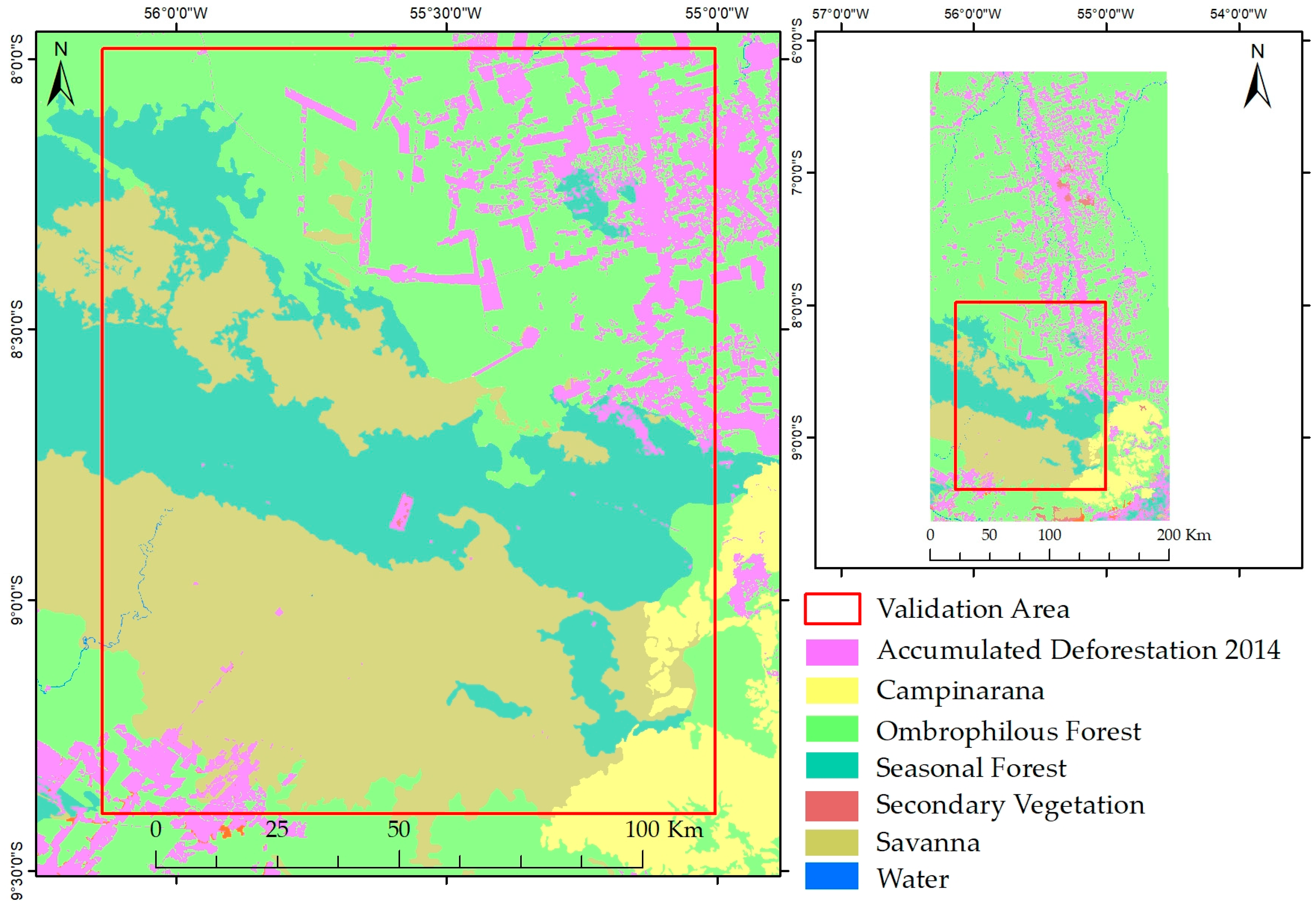
2. Study Area
3. Materials and Methods
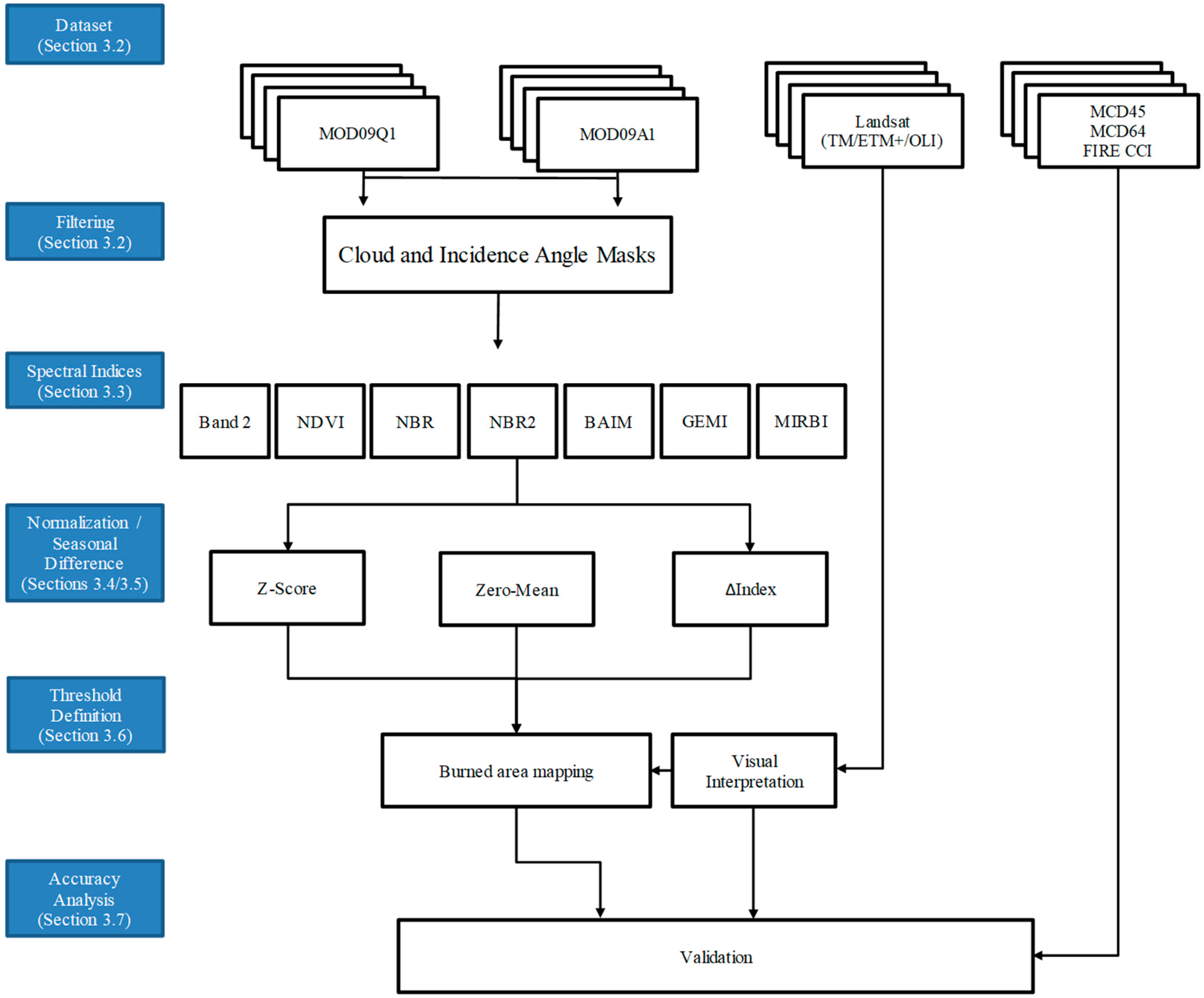
3.1. Methodology Flowchart
3.2. MODIS Data
3.3. Spectral Indices
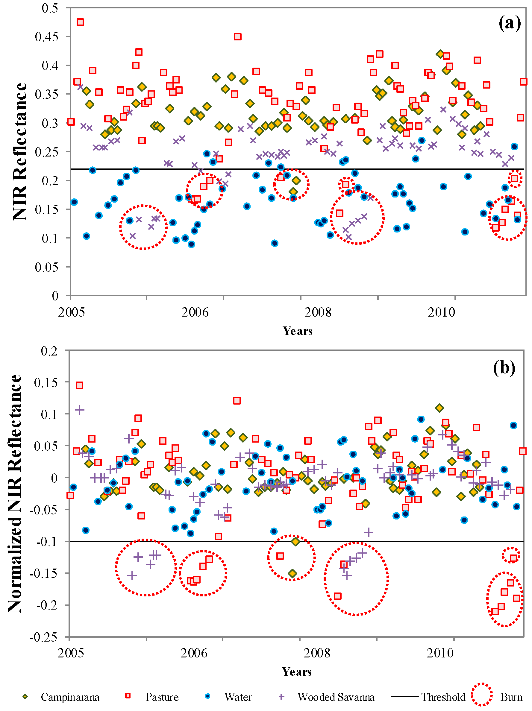
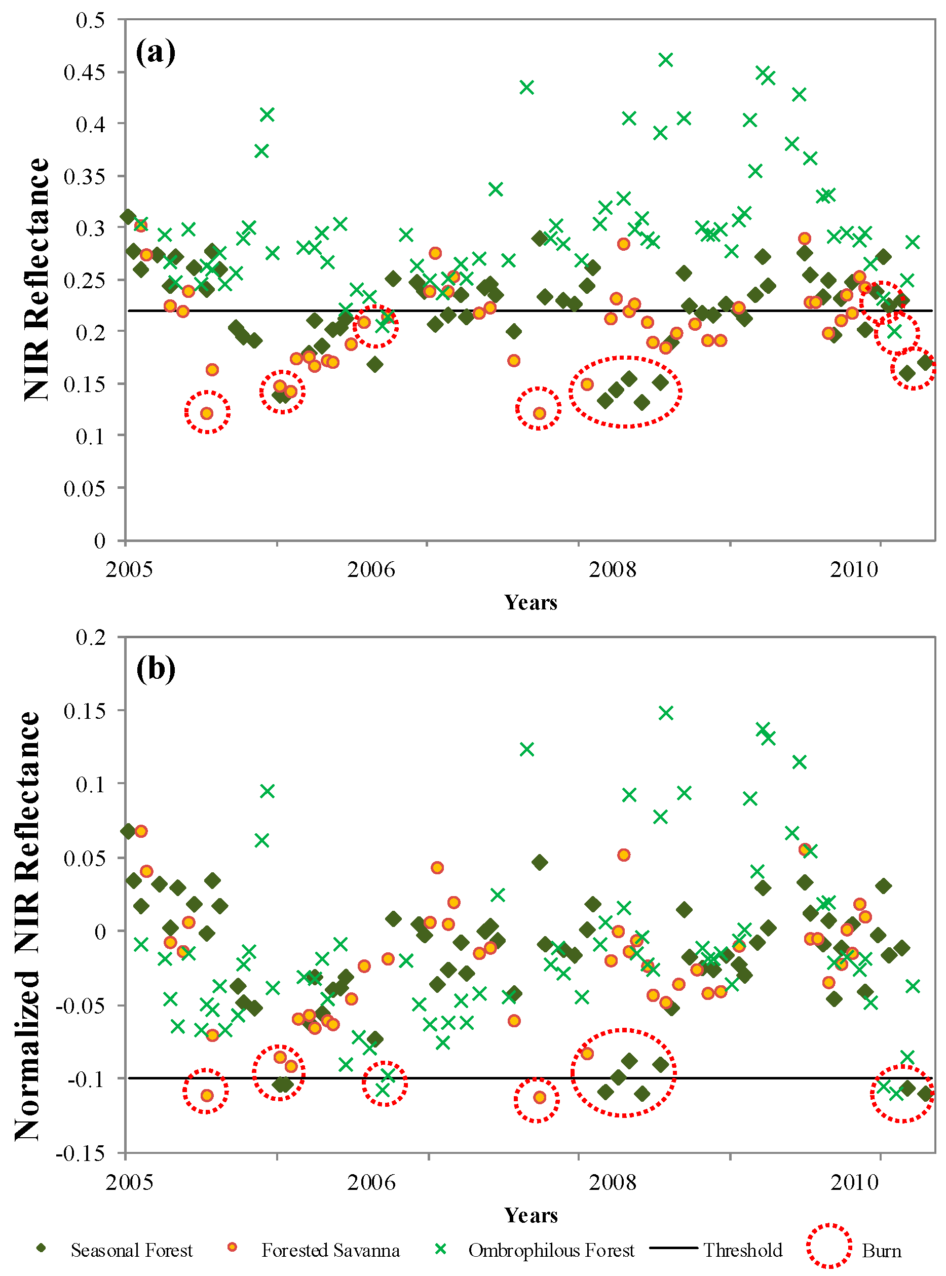
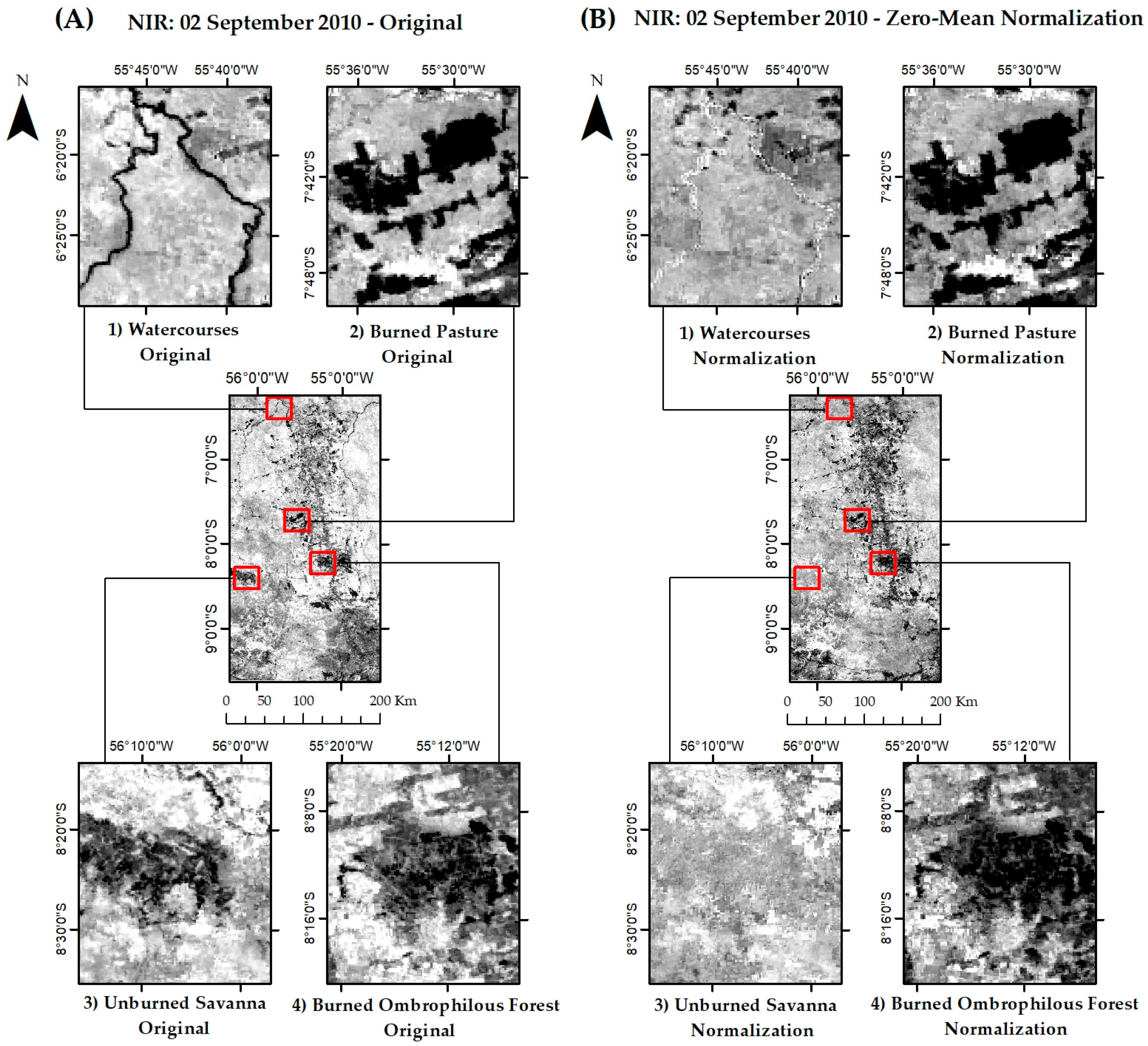
3.4. Time Series Standardization per Pixel
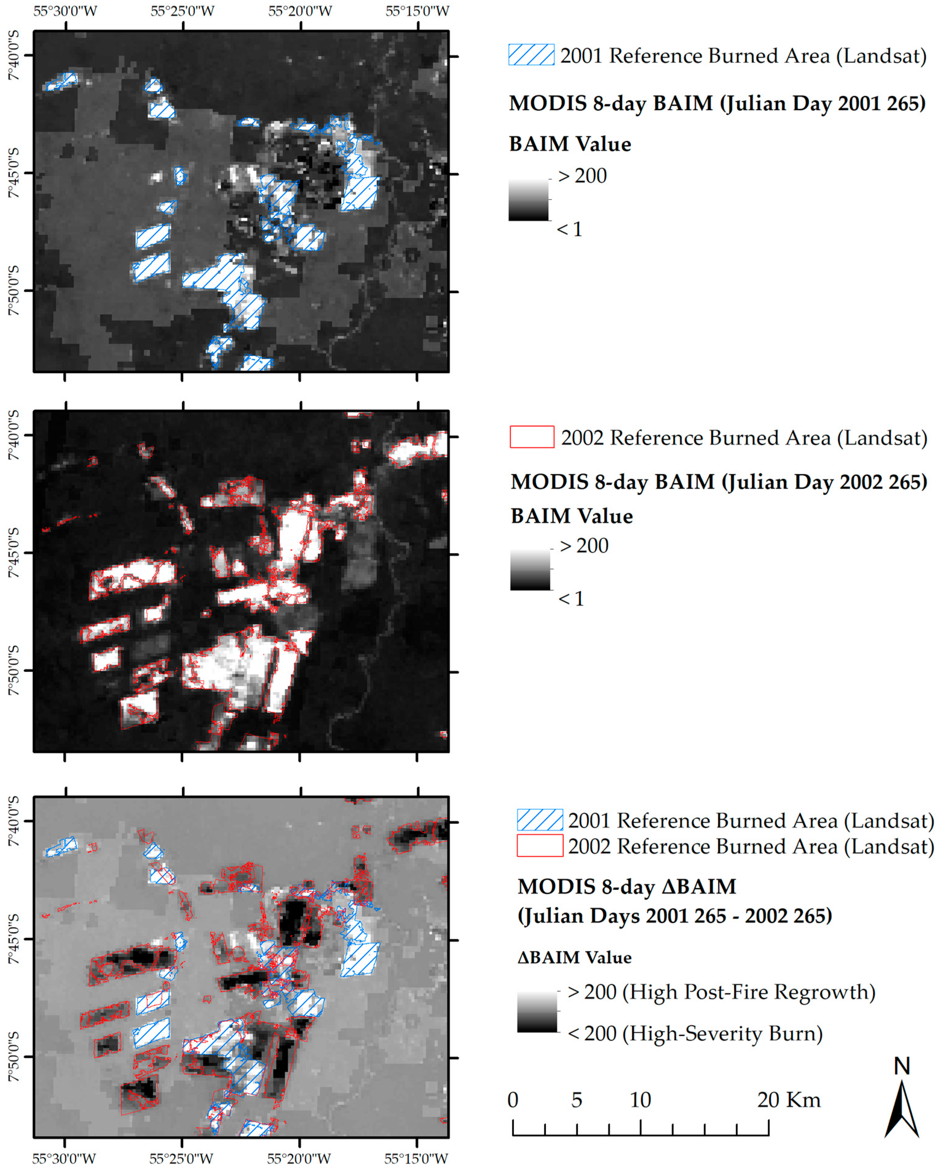
3.5. Seasonal Differencing
3.6. Landsat Reference Data and Burned Area Mapping
3.7. Dataset Comparison and Accuracy Analysis
3.8. Analysis of the Spatial Relationships between Land Use/Land Cover Classes and Burned Area
4. Results
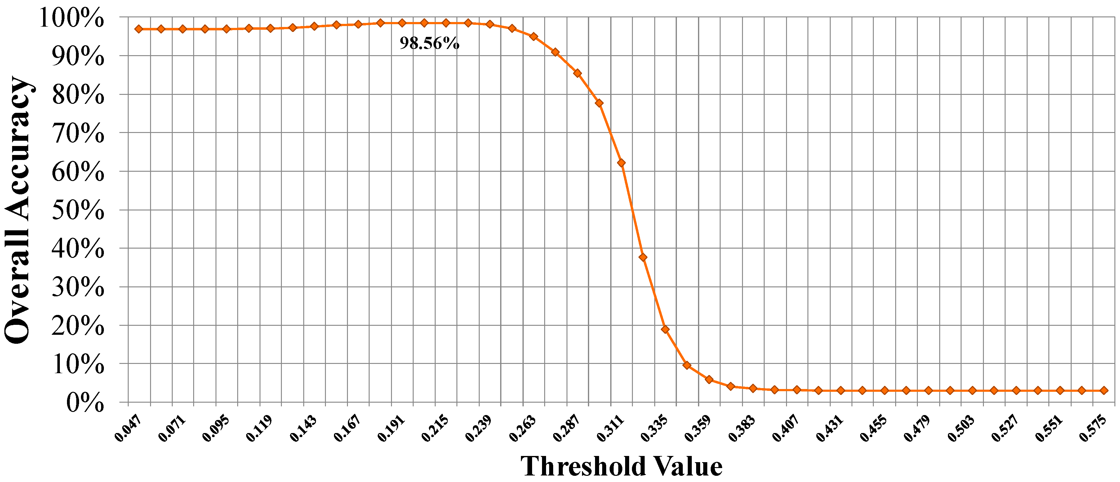
4.1. Determination of the Best Threshold Value
4.2. Validation and Data Comparison
4.3. Mapping Validation by Land Cover Type
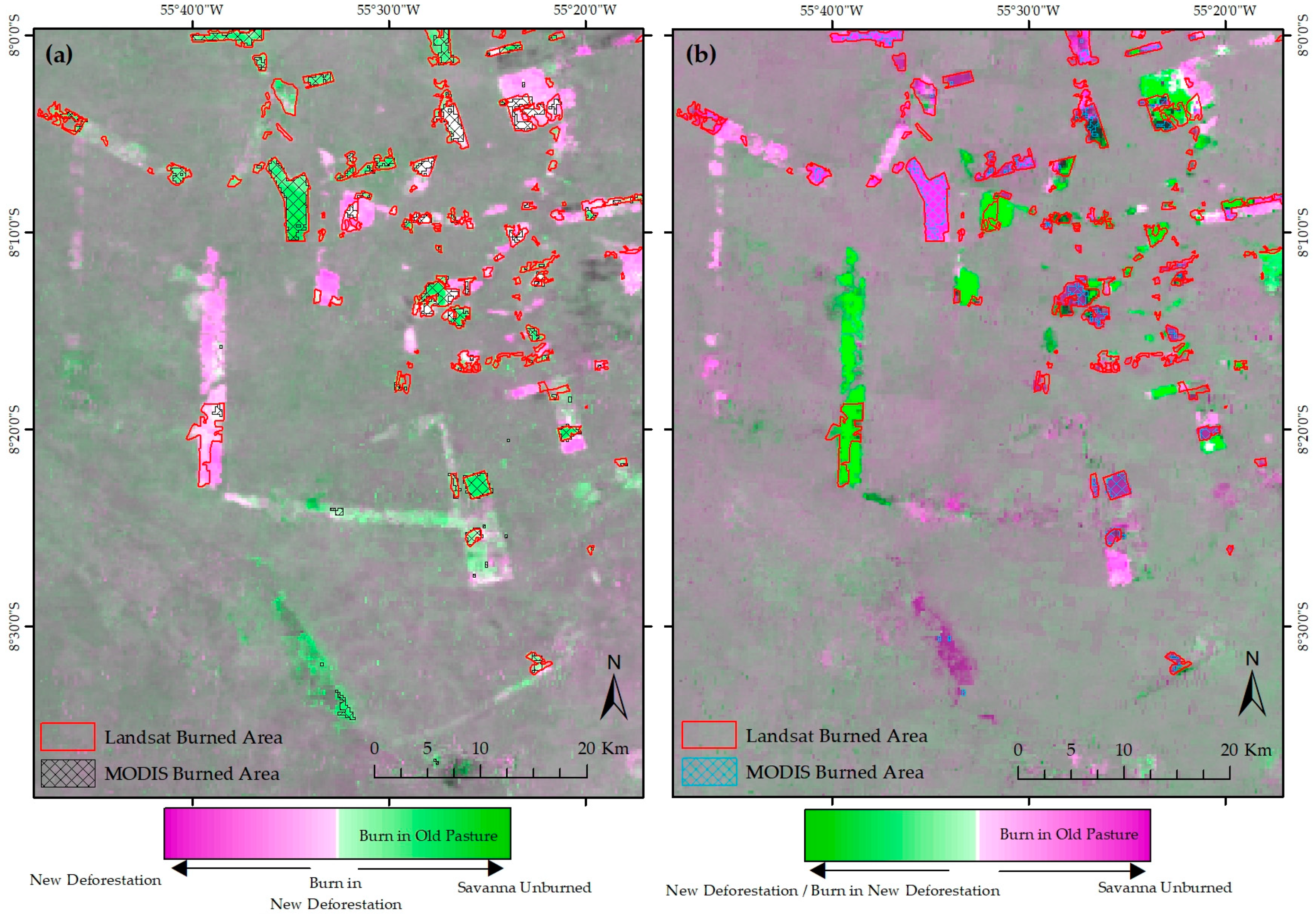
4.4. Land Use/Land Cover Classes and Burned Area Patterns
5. Discussion
6. Conclusions
Author Contributions
Funding
Acknowledgments
Conflicts of Interest
References
- Morton, D.C.; Defries, R.S.; Randerson, J.T.; Giglio, L.; Schroeder, W.; van der Werf, G.R. Agricultural intensification increases deforestation fire activity in Amazonia. Glob. Chang. Biol. 2008, 14, 2262–2275. [Google Scholar] [CrossRef] [Green Version]
- Cochrane, M.A. Synergistic interactions between habitat fragmentation and fire in evergreen tropical forests. Conserv. Biol. 2001, 15, 1515–1521. [Google Scholar] [CrossRef]
- Pivello, V.R. The use of fire in the cerrado and Amazonian rainforests of Brazil: Past and present. Fire Ecol. 2011, 7, 24–39. [Google Scholar] [CrossRef]
- Silvestrini, R.A.; Soares-Filho, B.S.; Nepstad, D.; Coe, M.; Rodrigues, H.; Assunção, R. Simulating fire regimes in the Amazon in response to climate change and deforestation. Ecol. Appl. 2011, 21, 1573–1590. [Google Scholar] [CrossRef] [PubMed]
- Cano-Crespo, A.; Oliveira, P.J.C.; Boit, A.; Cardoso, M.; Thonicke, K. Forest edge burning in the Brazilian Amazon promoted by escaping fires from managed pastures. J. Geophys. Res. G Biogeosci. 2015, 120, 2095–2107. [Google Scholar] [CrossRef]
- Nepstad, D.; Carvalho, G.; Barros, A.C.; Alencar, A.; Capobianco, J.P.; Bishop, J.; Moutinho, P.; Lefebvre, P.; Silva, U.L.; Prins, E. Road paving, fire regime feedbacks, and the future of Amazon forests. For. Ecol. Manag. 2001, 154, 395–407. [Google Scholar] [CrossRef]
- Nepstad, D.; Schwartzman, S.; Bamberger, B.; Santilli, M.; Ray, D.; Schlesinger, P.; Lefebvre, P.; Alencar, A.; Prinz, E.; Fiske, G.; et al. Inhibition of Amazon deforestation and fire by parks and indigenous lands. Conserv. Biol. 2006, 20, 65–73. [Google Scholar] [CrossRef] [PubMed]
- Cochrane, M.A.; Laurance, W.F. Fire as a large-scale edge effect in Amazonian forests. J. Trop. Ecol. 2002, 18, 311–325. [Google Scholar] [CrossRef]
- Alencar, A.A.; Brando, P.M.; Asner, G.P.; Putz, F.E. Landscape fragmentation, severe drought, and the new Amazon forest fire regime. Ecol. Appl. 2015, 25, 1493–1505. [Google Scholar] [CrossRef] [PubMed]
- van Marle, M.J.E.; Field, R.D.; van der Werf, G.R.; Estrada de Wagt, I.A.; Houghton, R.A.; Rizzo, L.V.; Artaxo, P.; Tsigaridis, K. Fire and deforestation dynamics in Amazonia (1973–2014). Glob. Biogeochem. Cycles 2016, 24–38. [Google Scholar] [CrossRef] [PubMed]
- Cochrane, M.A.; Schulze, M.D. Fire as a recurrent event in tropical forests of the eastern Amazon: Effects on forest structure, biomass, and species composition. Biotropica 1999, 31, 2–16. [Google Scholar] [CrossRef]
- Chuvieco, E.; Aguado, I.; Jurdao, S.; Pettinari, M.L.; Yebra, M.; Salas, J.; Hantson, S.; de la Riva, J.; Ibarra, P.; Rodrigues, M.; et al. Integrating geospatial information into fire risk assessment. Int. J. Wildl. Fire 2014, 23, 606–619. [Google Scholar] [CrossRef] [Green Version]
- Nepstad, D.C.; Verissimo, A.; Alencar, A.; Nobre, C.; Lima, E.; Lefebvre, P.; Schlesinger, P.; Potter, C.; Moutinho, P.; Mendoza, E.; et al. Large-scale impoverishment of Amazonian forests by logging and fire. Nature 1999, 398, 505–508. [Google Scholar] [CrossRef]
- Righi, C.A.; de Alencastro Graça, P.M.L.; Cerri, C.C.; Feigl, B.J.; Fearnside, P.M. Biomass burning in Brazil’s Amazonian “arc of deforestation”: Burning efficiency and charcoal formation in a fire after mechanized clearing at Feliz Natal, Mato Grosso. For. Ecol. Manag. 2009, 258, 2535–2546. [Google Scholar] [CrossRef]
- Lima, A.; Silva, T.S.F.; de Aragão, L.E.O.eC.; de Feitas, R.M.; Adami, M.; Formaggio, A.R.; Shimabukuro, Y.E. Land use and land cover changes determine the spatial relationship between fire and deforestation in the Brazilian Amazon. Appl. Geogr. 2012, 34, 239–246. [Google Scholar] [CrossRef]
- Laurance, W.F.; Bruce Williamson, G. Positive feedbacks among forest fragmentation, drought, and climate change in the Amazon. Conserv. Biol. 2001, 15, 1529–1535. [Google Scholar] [CrossRef]
- Phillips, O.L.; van der Heijden, G.; Lewis, S.L.; López-González, G.; Aragão, L.E.O.C.; Lloyd, J.; Malhi, Y.; Monteagudo, A.; Almeida, S.; Dávila, E.A.; et al. Drought-mortality relationships for tropical forests. New Phytol. 2010, 187, 631–646. [Google Scholar] [CrossRef] [PubMed] [Green Version]
- Nepstad, D.; Lefebvre, P.; Da Silva, U.L.; Tomasella, J.; Schlesinger, P.; Solórzano, L.; Moutinho, P.; Ray, D.; Benito, J.G. Amazon drought and its implications for forest flammability and tree growth: A basin-wide analysis. Glob. Chang. Biol. 2004, 10, 704–717. [Google Scholar] [CrossRef]
- Alencar, A.; Nepstad, D.; Del Carmen Vera Diaz, M. Forest understory fire in the Brazilian Amazon in ENSO and non-ENSO years: Area burned and committed carbon emissions. Earth Interact. 2006, 10. [Google Scholar] [CrossRef]
- Aragão, L.E.O.C.; Malhi, Y.; Roman-Cuesta, R.M.; Saatchi, S.; Anderson, L.O.; Shimabukuro, Y.E. Spatial patterns and fire response of recent Amazonian droughts. Geophys. Res. Lett. 2007, 34, 1–5. [Google Scholar] [CrossRef]
- Gutiérrez-Velez, V.H.; Uriarte, M.; Defries, R.; Pinedo-Vasquez, M.; Fernandes, K.; Ceccato, P.; Baethgen, W.; Padoch, C. Land cover change interacts with drought severity to change fire regimes in Western Amazonia. Ecol. Appl. 2014, 24, 1323–1340. [Google Scholar] [CrossRef] [PubMed]
- Asner, G.P. Cloud cover in Landsat observations of the Brazilian Amazon. Int. J. Remote Sens. 2001, 22, 3855–3862. [Google Scholar] [CrossRef]
- Lentile, L.B.; Holden, A.Z.A.; Smith, A.M.S.; Falkowski, M.J.; Hudak, A.T.; Morgan, P.; Lewis, S.A.; Gessler, P.E.; Benson, N.C. Remote sensing techniques to assess active fire characteristics and post-fire effects. Int. J. Wildl. Fire 2006, 15, 319–345. [Google Scholar] [CrossRef]
- Mouillot, F.; Schultz, M.G.; Yue, C.; Cadule, P.; Tansey, K.; Ciais, P.; Chuvieco, E. Ten years of global burned area products from spaceborne remote sensing—A review: Analysis of user needs and recommendations for future developments. Int. J. Appl. Earth Obs. Geoinf. 2014, 26, 64–79. [Google Scholar] [CrossRef] [Green Version]
- Huesca, M.; Litago, J.; Merino-de-Miguel, S.; Cicuendez-López-Ocaña, V.; Palacios-Orueta, A. Modeling and forecasting MODIS-based Fire Potential Index on a pixel basis using time series models. Int. J. Appl. Earth Obs. Geoinf. 2014, 26, 363–376. [Google Scholar] [CrossRef]
- Giglio, L.; Loboda, T.; Roy, D.P.; Quayle, B.; Justice, C.O. An active-fire based burned area mapping algorithm for the MODIS sensor. Remote Sens. Environ. 2009, 113, 408–420. [Google Scholar] [CrossRef]
- Bastarrika, A.; Chuvieco, E.; Martin, M.P. Automatic burned land mapping from MODIS time series images: Assessment in Mediterranean ecosystems. IEEE Trans. Geosci. Remote Sens. 2011, 49, 3401–3413. [Google Scholar] [CrossRef]
- Hardtke, L.A.; Blanco, P.D.; del Valle, H.F.; Metternicht, G.I.; Sione, W.F. Automated mapping of burned areas in semi-arid ecosystems using modis time-series imagery. ISPRS Int. Arch. Photogramm. Remote Sens. Spat. Inf. Sci. 2015, XL-7/W3, 811–814. [Google Scholar] [CrossRef]
- Giglio, L.; Csiszar, I.; Justice, C.O. Global distribution and seasonality of active fires as observed with the Terra and Aqua Moderate Resolution Imaging Spectroradiometer (MODIS) sensors. J. Geophys. Res. Biogeosci. 2006, 111, 1–12. [Google Scholar] [CrossRef]
- Justice, C.O.; Giglio, L.; Korontzi, S.; Owens, J.; Morisette, J.T.; Roy, D.; Descloitres, J.; Alleaume, S.; Petitcolin, F.; Kaufman, Y. The MODIS fire products. Remote Sens. Environ. 2002, 83, 244–262. [Google Scholar] [CrossRef]
- Roy, D.P.; Jin, Y.; Lewis, P.E.; Justice, C.O. Prototyping a global algorithm for systematic fire-affected area mapping using MODIS time series data. Remote Sens. Environ. 2005, 97, 137–162. [Google Scholar] [CrossRef]
- Vivchar, A.V.; Moiseenko, K.B.; Pankratova, N.V. Estimates of carbon monoxide emissions from wildfires in northern Eurasia for airquality assessment and climate modeling. Izv. Atmos. Ocean. Phys. 2010, 46, 281–293. [Google Scholar] [CrossRef]
- Vivchar, A. Wildfires in Russia in 2000–2008: Estimates of burnt areas using the satellite MODIS MCD45 data. Remote Sens. Lett. 2011, 2, 81–90. [Google Scholar] [CrossRef]
- Safronov, A.N.; Fokeeva, E.V.; Rakitin, V.S.; Grechko, E.I.; Shumsky, R.A. Severe wildfires near Moscow, Russia in 2010: Modeling of carbon monoxide pollution and comparisons with observations. Remote Sens. 2015, 7, 395–429. [Google Scholar] [CrossRef]
- Padilla, M.; Stehman, S.V.; Ramo, R.; Corti, D.; Hantson, S.; Oliva, P.; Alonso-Canas, I.; Bradley, A.V.; Tansey, K.; Mota, B.; et al. Comparing the accuracies of remote sensing global burned area products using stratified random sampling and estimation. Remote Sens. Environ. 2015, 160, 114–121. [Google Scholar] [CrossRef] [Green Version]
- Roy, D.P.; Boschetti, L.; Justice, C.O.; Ju, J. The collection 5 MODIS burned area product—Global evaluation by comparison with the MODIS active fire product. Remote Sens. Environ. 2008, 112, 3690–3707. [Google Scholar] [CrossRef]
- Anaya, J.A.; Chuvieco, E. Accuracy Assessment of Burned Area Products in the Orinoco Basin. Photogramm. Eng. Remote Sens. 2012, 7, 53–60. [Google Scholar] [CrossRef]
- Padilla, M.; Stehman, S.V.; Chuvieco, E. Validation of the 2008 MODIS-MCD45 global burned area product using stratified random sampling. Remote Sens. Environ. 2014, 144, 187–196. [Google Scholar] [CrossRef]
- Da Silva Cardozo, F.; Pereira, G.; Shimabukuro, Y.E.; Moraes, E.C. Validation of MODIS MCD45A1 product to identify burned areas in Acre State—Amazon forest. Int. Geosci. Remote Sens. Symp. 2012, 6741–6744. [Google Scholar] [CrossRef]
- Key, C.H.; Benson, N.C. Measuring and Remote Sensing of Burn Severity. In Proceedings of the U.S. Geological Survey Wildland Fire Workshop, Los Alamos, NM, USA, 31 October–3 November 2002. [Google Scholar]
- Rouse, J.W.; Haas, R.H.; Schell, J.A.; Deering, D.W.; Harlan, J.C. Monitoring the Vernal Advancement and Retrogradation (Green Wave Effect) of Natural Vegetation; Final Report; NASA/GSFC: Greenbelt, MD, USA, 1974.
- Kasischke, E.S.; French, N.H.F.; Harrel, P.; Christensen, N.L.; Ustin, S.L.; Barry, D. Monitoring of wildfires in boreal forest using large are AVHRR-NDVI composite image data. Remote Sens. Environ. 1993, 45, 61–71. [Google Scholar] [CrossRef]
- Martín, M.P.; Gómez, I.; Chuvieco, E. Burnt Area Index (BAIM) for burned area discrimination at regional scale using MODIS data. For. Ecol. Manag. 2006, 234, S221. [Google Scholar] [CrossRef]
- Pinty, B.; Verstraete, M.M. GEMI: A non-linear index to monitoring global vegetation from satellite. Vegetation 1992, 101, 15–20. [Google Scholar] [CrossRef]
- Trigg, S.; Flasse, S. An evaluation of different bi-spectral spaces for discriminating burned shrub-savannah. Int. J. Remote Sens. 2001, 22, 2641–2647. [Google Scholar] [CrossRef]
- Key, C.H.; Benson, N.C. Landscape Assessment: Sampling and Analysis Methods; USDA For. Serv. Gen. Tech. Rep. RMRS-GTR-164-CD; USDA Forest Service: Washington, DC, USA, 2006; pp. 1–55. [Google Scholar]
- Loboda, T.; O’Neal, K.J.; Csiszar, I. Regionally adaptable dNBR-based algorithm for burned area mapping from MODIS data. Remote Sens. Environ. 2007, 109, 429–442. [Google Scholar] [CrossRef]
- Veraverbeke, S.; Lhermitte, S.; Verstraeten, W.W.; Goossens, R. The temporal dimension of differenced Normalized Burn Ratio (dNBR) fire/burn severity studies: The case of the large 2007 Peloponnese wildfires in Greece. Remote Sens. Environ. 2010, 114, 2548–2563. [Google Scholar] [CrossRef] [Green Version]
- Lhermitte, S.; Verbesselt, J.; Verstraeten, W.W.; Veraverbeke, S.; Coppin, P. Assessing intra-annual vegetation regrowth after fire using the pixel based regeneration index. ISPRS J. Photogramm. Remote Sens. 2011, 66, 17–27. [Google Scholar] [CrossRef] [Green Version]
- Diaz-Delgado, R.; Salvador, R.; Pons, X. Monitoring of plant community regeneration after fire by remote sensing. In Fire Management and Landscape Ecology; Traboud, L., Ed.; International Association of Wildland Fire: Fairfield, WA, USA, 1998; pp. 315–324. [Google Scholar]
- Instituto Brasileiro de Geografia e Estatística (IBGE) Mapa de Climas do Brasil. Available online: http://portaldemapas.ibge.gov.br (accessed on 23 October 2015).
- Instituto Nacional de Meteorologia (Inmet) Normais Climatológicas do Brasil. Available online: http://www.inmet.gov.br (accessed on 23 October 2015).
- Instituto Nacional de Pesquisas Espaciais (INPE) Portal do Monitoramento de Queimadas e Incêndios. Available online: http://queimadas.cptec.inpe.br (accessed on 22 June 2015).
- Instituto Nacional de Pesquisas Espaciais (INPE) Monitoramento da Floresta Amazônica Brasileira por Satélite—Projeto PRODES. Available online: http://www.obt.inpe.br/prodes (accessed on 25 October 2015).
- Instituto Brasileiro de Geografia e Estatística (IBGE) Vegetação: Estado do Pará. Available online: http://portaldemapas.ibge.gov.br (accessed on 23 October 2015).
- Instituto Chico Mendes de Conservação da Biodiversidade (ICMBIO) Geoprocessamento. Available online: http://www.icmbio.gov.br (accessed on 25 October 2015).
- Fundação Nacional do Índio (FUNAI) Mapas. Available online: http://mapas2.funai.gov.br (accessed on 24 October 2015).
- Instituto Nacional de Colonização e Reforma Agrária (INCRA) Acervo Fundiário. Available online: http://acervofundiario.incra.gov.br (accessed on 25 October 2015).
- Instituto do Homem e Meio Ambiente da Amazônia (IMAZON) Mapas—Áreas Protegidas da Amazônia Legal. Available online: http://imazon.org.br (accessed on 25 October 2015).
- Zimmerman, B.; Peres, C.A.; Malcolm, J.R.; Turner, T. Conservation and development alliances with the Kayapó of south-eastern Amazonia, a tropical forest indigenous people. Environ. Conserv. 2001, 28, 10–22. [Google Scholar] [CrossRef]
- Fearnside, P.M. Brazil’s Cuiabá- Santarém (BR-163) Highway: The environmental cost of paving a soybean corridor through the Amazon. Environ. Manag. 2007, 39, 601–614. [Google Scholar] [CrossRef] [PubMed]
- Chuvieco, E.; Pettinari, M.L.; Heil, A.; Storm, T. ESA Climate Change Initiative—Fire Disturbance: D1.2 Product Specification Report; Version 6.1; University of Alcala: Spain, 2016. [Google Scholar]
- Alonso-Canas, I.; Chuvieco, E. Global burned area mapping from ENVISAT-MERIS and MODIS active fire data. Remote Sens. Environ. 2015, 163, 140–152. [Google Scholar] [CrossRef]
- Justice, C.O.; Townshend, J.R.G.; Vermote, E.F.; Masuoka, E.; Wolfe, R.E.; Saleous, N.; Roy, D.P.; Morisette, J.T. An overview of MODIS Land data processing and product status. Remote Sens. Environ. 2002, 83, 3–15. [Google Scholar] [CrossRef] [Green Version]
- Vermote, E.F. MOD09A1 MODIS Surface Reflectance 8-Day L3 Global 500m SIN Grid V006; NASA LP DAAC: Sioux Falls, SD, USA, 2016. [CrossRef]
- Chuvieco, E.; Ventura, G.; Martín, M.P.; Gómez, I. Assessment of multitemporal compositing techniques of MODIS and AVHRR images for burned land mapping. Remote Sens. Environ. 2005, 94, 450–462. [Google Scholar] [CrossRef]
- Morton, D.C.; Nagol, J.; Carabajal, C.C.; Rosette, J.; Palace, M.; Cook, B.D.; Vermote, E.F.; Harding, D.J.; North, P.R.J. Amazon forests maintain consistent canopy structure and greenness during the dry season. Nature 2014, 506, 1–16. [Google Scholar] [CrossRef] [PubMed]
- Maier, S.W. Changes in surface reflectance from wildfires on the Australian continent measured by MODIS. Int. J. Remote Sens. 2010, 31, 3161–3176. [Google Scholar] [CrossRef]
- Pereira, J.M.C.; Sa, A.C.L.; Souza, A.M.O.; Silva, J.M.N.; Santos, T.N.; Carreiras, J.M. Spectral characterization and discrimination of burnt areas. In Remote Sensing of Large Wildfires in the European Mediterranean Basin; Springer: Berlin, Germany, 1999; pp. 123–138. [Google Scholar]
- Forkel, M.; Carvalhais, N.; Verbesselt, J.; Mahecha, M.D.; Neigh, C.S.R.; Reichstein, M. Trend Change detection in NDVI time series: Effects of inter-annual variability and methodology. Remote Sens. 2013, 5, 2113–2144. [Google Scholar] [CrossRef]
- Kolden, C.; Roganf, J. Mapping Wildfire Burn Severity in the Arctic Tundra from Downsampled MODIS Data. Arct. Antarct Alp. Res. 2013, 45, 64–76. [Google Scholar] [CrossRef]
- Godwin, D.R.; Kobziar, L.N. Comparison of burn severities of consecutive large-scale fires in Florida sand pine scrubusing satellite imagery analysis. Fire Ecol. 2011, 7, 99–113. [Google Scholar] [CrossRef]
- Chen, X.; Vogelmann, J.E.; Rollins, M.; Ohlen, D.; Key, C.H.; Yang, L.; Huang, C.; Shi, H. Detecting post-fire burn severity and vegetation recovery using multitemporal remote sensing spectral indices and field-collected composite burn index data in a ponderosa pine forest. Int. J. Remote Sens. 2011, 32, 7905–7927. [Google Scholar] [CrossRef]
- Zidane, I.; Lhissou, R.; Bouli, A.; Mabrouki, M. An improved algorithm for mapping burnt areas in the Mediterranean forest landscape of Morocco. J. For. Res. 2018. [Google Scholar] [CrossRef]
- Holden, Z.A.; Morgan, P.; Smith, A.M.S.; Vierling, L. Beyond Landsat: A comparison of four satellite sensors for detecting burn severity in ponderosa pine forests of the Gila Wilderness, NM, USA. Int. J. Wildl. Fire 2010, 19, 449–458. [Google Scholar] [CrossRef]
- Hislop, S.; Jones, S.; Soto-Berelov, M.; Skidmore, A.; Haywood, A.; Nguyen, T.H. Using landsat spectral indices in time-series to assess wildfire disturbance and recovery. Remote Sens. 2018, 10, 460. [Google Scholar] [CrossRef]
- Dempewolf, J.; Trigg, S.; DeFries, R.S.; Eby, S. Burned-Area Mapping of the Serengeti–Mara Region Using MODIS Reflectance Data. IEEE Geosci. Remote Sens. Lett. 2007, 4, 312–316. [Google Scholar] [CrossRef]
- McCarley, T.R.; Smith, A.M.S.; Kolden, C.A.; Kreitler, J. Evaluating the Mid-Infrared Bi-spectral Index for improved assessment of low-severity fire effects in a conifer forest. Int. J. Wildl. Fire 2018, 27, 407. [Google Scholar] [CrossRef]
- García, M.J.L.; Caselles, V. Mapping burns and natural reforestation using thematic Mapper data. Geocarto Int. 1991, 6, 31–37. [Google Scholar] [CrossRef]
- Pereira, J.M.C. Remote sensing of burned areas in tropical savannas. Int. J. Wildl. Fire 2003, 12, 259. [Google Scholar] [CrossRef]
- Cardozo, S.; Pereira, G.; Shimabukuro, Y.E.; Moraes, E.C. Avaliação Das Áreas Queimadas No Estado De Rondônia. Rev. Bras. Cartogr. 2014, 66, 705–716. [Google Scholar]
- Shimabukuro, Y.E.; Duarte, V.; Arai, E.; Freitas, R.M.; Lima, A.; Valeriano, D.M.; Brown, I.F.; Maldonado, M.L.R. Fraction images derived from Terra Modis data for mapping burnt areas in Brazilian Amazonia. Int. J. Remote Sens. 2009, 30, 1537–1546. [Google Scholar] [CrossRef]
- De Carvalho Júnior, O.A.; Guimarães, R.F.; Silva, C.; Gomes, R.A.T. Standardized Time-Series and Interannual Phenological Deviation: New Techniques for Burned-Area Detection Using Long-Term MODIS-NBR Dataset. Remote Sens. 2015, 7, 6950–6985. [Google Scholar] [CrossRef] [Green Version]
- Lhermitte, S.; Verbesselt, J.; Verstraeten, W.W.; Coppin, P. A Pixel Based Regeneration Index using Time Series Similarity and Spatial Context. Photogramm. Eng. Remote Sens. 2010, 76, 673–682. [Google Scholar] [CrossRef]
- Veraverbeke, S.; Somers, B.; Gitas, I.; Katagis, T.; Polychronaki, A.; Goossens, R. Spectral mixture analysis to assess post-fire vegetation regeneration using Landsat Thematic Mapper imagery: Accounting for soil brightness variation. Int. J. Appl. Earth Obs. Geoinf. 2012, 14, 1–11. [Google Scholar] [CrossRef] [Green Version]
- Roy, D.P.; Boschetti, L. Southern Africa validation of the MODIS, L3JRC, and GlobCarbon burned-area products. IEEE Trans. Geosci. Remote Sens. 2009, 47, 1032–1044. [Google Scholar] [CrossRef]
- Eva, H.; Lambin, E.F. Fires and land-cover change in the tropics:a remote sensing analysis at the landscape scale. J. Biogeogr. 2000, 27, 765–776. [Google Scholar] [CrossRef]
- Parrini, F.; Owen-Smith, N. The importance of post-fire regrowth for sable antelope in a Southern African savanna. Afr. J. Ecol. 2010, 48, 526–534. [Google Scholar] [CrossRef]
- Padilla, M.; Stehman, S.V.; Litago, J.; Chuvieco, E. Assessing the temporal stability of the accuracy of a time series of burned area products. Remote Sens. 2014, 6, 2050–2068. [Google Scholar] [CrossRef]
- Congalton, R.G. A review of assessing the accuracy of classifications of remotely sensed data. Remote Sens. Environ. 1991, 37, 35–46. [Google Scholar] [CrossRef]
- Fleiss, J.L.; Levin, B.; Paik, M.C. Statistical Methods for Rates and Proportions; Wiley Series in Probability and Statistics; John Wiley & Sons, Inc.: Hoboken, NJ, USA, 2003. [Google Scholar]
- Arvidson, T.; Goward, S.N.; Gasch, J.; Williams, D. Landsat-7 long-term acquisition plan: Development and validation. Photogramm. Eng. Remote Sens. 2006, 72, 1137–1146. [Google Scholar] [CrossRef]
- McNemar, Q. Note on the sampling error of the difference between correlated proportions or percentages. Psychometrika 1947, 12, 153–157. [Google Scholar] [CrossRef] [PubMed]
- Foody, G.M. Thematic map comparison: Evaluating the statistical significance of differences in classification accuracy. Photogramm. Eng. Remote Sens. 2004, 70, 627–633. [Google Scholar] [CrossRef]
- Quintano, C.; Fernández-Manso, A.; Fernández-Manso, O. Combination of Landsat and Sentinel-2 MSI data for initial assessing of burn severity. Int. J. Appl. Earth Obs. Geoinf. 2018, 64, 221–225. [Google Scholar] [CrossRef] [Green Version]
- Pleniou, M.; Koutsias, N. Sensitivity of spectral reflectance values to different burn and vegetation ratios: A multi-scale approach applied in a fire affected area. ISPRS J. Photogramm. Remote Sens. 2013, 79, 199–210. [Google Scholar] [CrossRef]
- Roy, D.P.; Boschetti, L.; Trigg, S.N. Remote sensing of fire severity: Assessing the performance of the normalized burn ratio. IEEE Geosci. Remote Sens. Lett. 2006, 3, 112–116. [Google Scholar] [CrossRef]
- Quintano, C.; Fernández-Manso, A.; Stein, A.; Bijker, W. Estimation of area burned by forest fires in Mediterranean countries: A remote sensing data mining perspective. For. Ecol. Manag. 2011, 262, 1597–1607. [Google Scholar] [CrossRef]
- Chen, Y.; Morton, D.C.; Jin, Y.; Collatz, G.J.; Kasibhatla, P.S.; van der Werf, G.R.; DeFries, R.S.; Randerson, J.T.; Gollatz, G.J.; Kasibhatla, P.S.; et al. Long-term trends and interannual variability of forest, savanna and agricultural fires in South America. Carbon Manag. 2013, 4, 617–638. [Google Scholar] [CrossRef] [Green Version]
- Libonati, R.; DaCamara, C.C.; Setzer, A.W.; Morelli, F.; Melchiori, A.E. An algorithm for burned area detection in the Brazilian Cerrado using 4 μm MODIS imagery. Remote Sens. 2015, 7, 15782–15803. [Google Scholar] [CrossRef]
- De Mendonça, M.J.C.; Vera Diaz, M.D.C.; Nepstad, D.; Seroa Da Motta, R.; Alencar, A.; Gomes, J.C.; Ortiz, R.A. The economic cost of the use of fire in the Amazon. Ecol. Econ. 2004, 49, 89–105. [Google Scholar] [CrossRef]
- Nelson, A.; Chomitz, K.M. Effectiveness of strict vs. multiple use protected areas in reducing tropical forest fires: A global analysis using matching methods. PLoS ONE 2011, 6. [Google Scholar] [CrossRef] [PubMed]
- Quintano, C.; Fernández-Manso, A.; Fernández-Manso, O.; Shimabukuro, Y.E. Mapping burned areas in Mediterranean countries using spectral mixture analysis from a uni-temporal perspective. Int. J. Remote Sens. 2006, 27, 645–662. [Google Scholar] [CrossRef]
- Quintano, C.; Fernández-Manso, A.; Roberts, D.A. Multiple Endmember Spectral Mixture Analysis (MESMA) to map burn severity levels from Landsat images in Mediterranean countries. Remote Sens. Environ. 2013, 136, 76–88. [Google Scholar] [CrossRef]
- Cao, X.; Chen, J.; Matsushita, B.; Imura, H.; Wang, L. An automatic method for burn scar mapping using support vector machines. Int. J. Remote Sens. 2009, 30, 577–594. [Google Scholar] [CrossRef]
- Dragozi, E.; Gitas, I.; Stavrakoudis, D.; Theocharis, J. Burned Area Mapping Using Support Vector Machines and the FuzCoC Feature Selection Method on VHR IKONOS Imagery. Remote Sens. 2014, 6, 12005–12036. [Google Scholar] [CrossRef] [Green Version]


| Index | Equation | Bibliographic Reference |
|---|---|---|
| NBR/ΔNBR | [40,79] | |
| NDVI/ΔNDVI | [41] | |
| NBR2/ΔNBR2 | [46] | |
| BAIM/ΔBAIM | [43] | |
| GEMI/ΔGEMI | [44] | |
| MIRBI/ΔMIRBI | [45] | |
| Δ |
| Image Date | Sensor | Percentage of Low-Quality Pixels | ||
|---|---|---|---|---|
| Normalization Method | Seasonal Difference (Fixed Interval) | Seasonal Difference (Closest High-Quality Image) | ||
| 15/08/2001 | ETM+ | 34% | - | - |
| 19/09/2002 | ETM+ | 25% | 77% | 19% |
| 28/07/2003 | TM | 13% | 82% | 24% |
| 30/07/2004 | TM | 44% | 51% | 13% |
| 03/09/2005 | TM | 26% | 51% | 12% |
| 10/08/2008 | TM | 47% | 57% | 45% |
| 01/09/2010 | TM | 7% | 49% | 22% |
| True Condition (Landsat Classification) | |||
|---|---|---|---|
| Burned Area | Unburned Area | ||
| Predicted Condition (MODIS Classification) | Burned area | True Positive (TP) | False Positive (FP) |
| Unburned area | False Negative (FN) | True Negative (TN) | |
| Classification 2 | |||
|---|---|---|---|
| Correct | Incorrect | Total | |
| Classification 1 | |||
| Correct | f11 | f12 | f11 + f12 |
| Incorrect | f21 | f22 | f21 + f22 |
| Total | f11 + f21 | f12 + f22 | f11 + f12 + f21 + f22 |
| Original Data | |||||||
| BAIM | Band 2 | GEMI | MIRBI | NBR | NBR2 | NDVI | |
| Threshold | 17.48 | 0.206 | 0.560 | 1.312 | 0.148 | 0.230 | 0.480 |
| OA | 97.1% | 97.0% | 97.0% | 97.0% | 96.3% | 96.7% | 96.0% |
| Seasonal Difference (Δ = Pre-fire − Post-fire) | |||||||
| ΔBAIM | ΔBand 2 | ΔGEMI | ΔMIRBI | ΔNBR | ΔNBR2 | ΔNDVI | |
| Threshold | −31.2 | 0.04 | 0.11 | −0.25 | 0.22 | 0.12 | 0.22 |
| OA | 98.7% | 98.2% | 98.3% | 98% | 98.2% | 98.4% | 98.3% |
| Seasonal Difference (Δ = Pre-fire − Post-fire) with selected images by quality next to birthday | |||||||
| ΔBAIM | ΔBand 2 | ΔGEMI | ΔMIRBI | ΔNBR | ΔNBR2 | ΔNDVI | |
| Threshold | −28.32 | 0.041 | 0.156 | −0.406 | 0.278 | 0.138 | 0.172 |
| OA | 97.2% | 97.1% | 97.0% | 97.0% | 96.7% | 96.5% | 96.5% |
| Z-score normalization | |||||||
| BAIM | Band 2 | GEMI | MIRBI | NBR | NBR2 | NDVI | |
| Threshold | 1.235 | −1.744 | −1.825 | 1.430 | −1.925 | −1.428 | −1.918 |
| OA | 97.1% | 97.4% | 97.2% | 97.0% | 96.5% | 96.5% | 96.0% |
| Zero-mean normalization | |||||||
| BAIM | Band 2 | GEMI | MIRBI | NBR | NBR2 | NDVI | |
| Threshold | 11 | −0.109 | −0.200 | 0.250 | −0.284 | −0.160 | −0.203 |
| OA | 97.8% | 97.9% | 97.7% | 97.3% | 96.9% | 96.9% | 96.8% |
| Original Data | |||||||
| BAIM | Band 2 | GEMI | MIRBI | NBR | NBR2 | NDVI | |
| DC | 0.588 | 0.527 | 0.337 | 0.326 | 0.422 | 0.430 | 0.399 |
| OA | 98.56% | 98.71% | 98.36% | 98.31% | 98.30% | 97.71% | 96.81% |
| Commission Errors | 48.02% | 34.21% | 20.75% | 27.44% | 34.40% | 61.99% | 46.06% |
| Omission Errors | 38.20% | 53.75% | 79.96% | 76.95% | 62.60% | 45.49% | 38.02% |
| Seasonal Difference (Pre-fire − Post-fire) with fixed interval | |||||||
| ΔBAIM | ΔBand 2 | ΔGEMI | ΔMIRBI | ΔNBR | ΔNBR2 | ΔNDVI | |
| DC | 0.506 | 0.485 | 0.384 | 0.334 | 0.428 | 0.412 | 0.400 |
| OA | 98.15% | 97.87% | 97.11% | 96.59% | 97.51% | 97.50% | 97.15% |
| Commission Errors | 29.82% | 71.67% | 40.71% | 42. 37% | 51.22% | 54.21% | 69.47% |
| Omission Errors | 62.60% | 42.85% | 73. 57% | 74.02% | 61.23% | 62.01% | 59.41% |
| Seasonal Difference (Pre-fire − Post-fire) with selected images | |||||||
| ΔBAIM | ΔBand 2 | ΔGEMI | ΔMIRBI | ΔNBR | ΔNBR2 | ΔNDVI | |
| DC | 0.592 | 0.606 | 0.481 | 0.357 | 0.537 | 0.487 | 0.425 |
| OA | 98.69% | 98.74% | 98.57% | 98.49% | 98.62% | 98.52% | 97.23% |
| Commission Errors | 14.86% | 32.30% | 17.98% | 25.56% | 23.14% | 35.46% | 40.22% |
| Omission Errors | 48.43% | 38.71% | 64.98% | 76.45% | 57.50% | 58.50% | 46.72% |
| Z-score normalization | |||||||
| BAIM | Band 2 | GEMI | MIRBI | NBR | NBR2 | NDVI | |
| DC | 0.591 | 0.618 | 0.476 | 0.501 | 0.429 | 0.452 | 0.397 |
| OA | 98.38% | 98.80% | 98.54% | 98.44% | 98.69% | 97.73% | 96.38% |
| Commission Errors | 45.42% | 38.97% | 34.16% | 35.80% | 45.77% | 47.23% | 56.81% |
| Omission Errors | 39.36% | 38.70% | 62.58% | 55.90% | 45.45% | 45.74% | 45.59% |
| Zero-mean normalization | |||||||
| BAIM | Band 2 | GEMI | MIRBI | NBR | NBR2 | NDVI | |
| DC | 0.625 | 0.647 | 0.566 | 0.539 | 0.508 | 0.503 | 0.479 |
| OA | 98.36% | 98.99% | 98.44% | 98.59% | 98.66% | 98.31% | 97.54% |
| Commission Errors | 38.01% | 32.41% | 28.29% | 33.21% | 35.55% | 46.61% | 48.60% |
| Omission Errors | 31.64% | 34.75% | 55.20% | 49.60% | 42.69% | 42.48% | 30.96% |
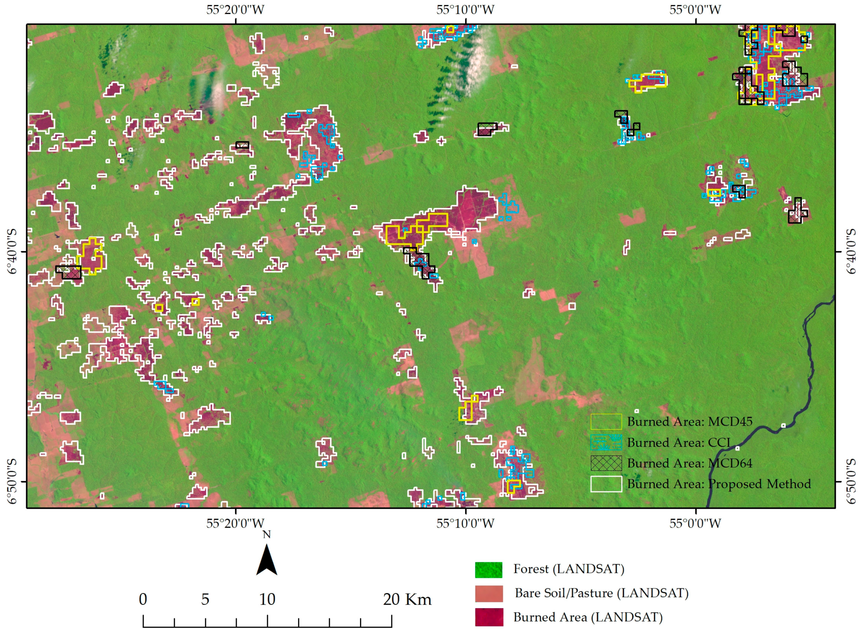
| Burned Area Product | Overall Accuracy | Dice Coefficient | Commission Errors | Omission Errors |
|---|---|---|---|---|
| MCD45 | 98.58% | 0.11 | 24.34% | 93.55% |
| MCD64 | 98.61% | 0.24 | 23.83% | 84.51% |
| FIRE_CCI | 98.48% | 0.09 | 24.89% | 94.67% |
| Land Cover | Overall Accuracy | Dice Coefficient | Commission Errors | Omission Errors |
|---|---|---|---|---|
| Campinarana | 99.25% | 0.778 | 9.71% | 27.60% |
| Deforestation/Pasture | 99.19% | 0.755 | 18.57% | 34.76% |
| Ombrophilous Forest | 98.68% | 0.506 | 23.40% | 49.62% |
| Savanna | 98.62% | 0.466 | 59.25% | 37.42% |
| Seasonal Forest | 98.57% | 0.371 | 23.23% | 76.85% |
| Area (km2) | |||||||
|---|---|---|---|---|---|---|---|
| Year | CP | D/P | OF | S | SF | SV | |
| 2001 | 14.16 (0.5%) | 280.66 (6.9%) | 49.56 (0.1%) | 2.55 (0.03%) | 12.18 (0.2%) | 0.28 (0.1%) | |
| 2002 | 12.84 (0.4%) | 773.68 (14.4%) | 84.08 (0.2%) | 14.61 (0.18%) | 12.77 (0.2%) | 0.78 (0.2%) | |
| 2003 | 26.82 (0.9%) | 497.05 (8.2%) | 92.58 (0.2%) | 9.06 (0.11%) | 18.24 (0.3%) | 1.05 (0.3%) | |
| 2004 | 51.60 (1.7%) | 1203.22 (16.8%) | 235.74 (0.5%) | 15.58 (0.19%) | 20.14 (0.3%) | 0.12 (0.0%) | |
| 2005 | 33.10 (1.1%) | 771.25 (9.9%) | 111.60 (0.2%) | 15.38 (0.19%) | 23.97 (0.4%) | 0.86 (0.3%) | |
| 2006 | 26.85 (0.9%) | 781.16 (9.4%) | 244.92 (0.5%) | 22.15 (0.28%) | 70.80 (1.1%) | 1.52 (0.5%) | |
| 2007 | 18.24 (0.6%) | 677.03 (7.6%) | 143.28 (0.3%) | 5.21 (0.06%) | 22.24 (0.3%) | 0.20 (0.1%) | |
| 2008 | 41.48 (1.4%) | 625.33 (6.6%) | 130.02 (0.3%) | 28.77 (0.36%) | 44.52 (0.7%) | 1.37 (0.4%) | |
| 2009 | 15.19 (0.5%) | 233.87 (2.3%) | 121.21 (0.3%) | 4.53 (0.06%) | 52.62 (0.8%) | 0.43 (0.1%) | |
| 2010 | 7.21 (0.2%) | 749.36 (7.2%) | 196.83 (0.4%) | 11.10 (0.14%) | 23.60 (0.4%) | 1.62 (0.5%) | |
| 2011 | 23.66 (0.8%) | 214.61 (2.0%) | 90.71 (0.2%) | 5.95 (0.07%) | 15.54 (0.2%) | 0.66 (0.2%) | |
| 2012 | 4.49 (0.1%) | 395.61 (3.5%) | 87.07 (0.2%) | 2.78 (0.03%) | 13.08 (0.2%) | 0.40 (0.1%) | |
| 2013 | 10.77 (0.4%) | 166.01 (1.4%) | 47.75 (0.1%) | 3.30 (0.04%) | 6.06 (0.1%) | 0.25 (0.1%) | |
| 2014 | 5.65 (0.2%) | 748.24 (6.2%) | 102.40 (0.2%) | 3.18 (0.04%) | 16.60 (0.3%) | 2.06 (0.6%) | |
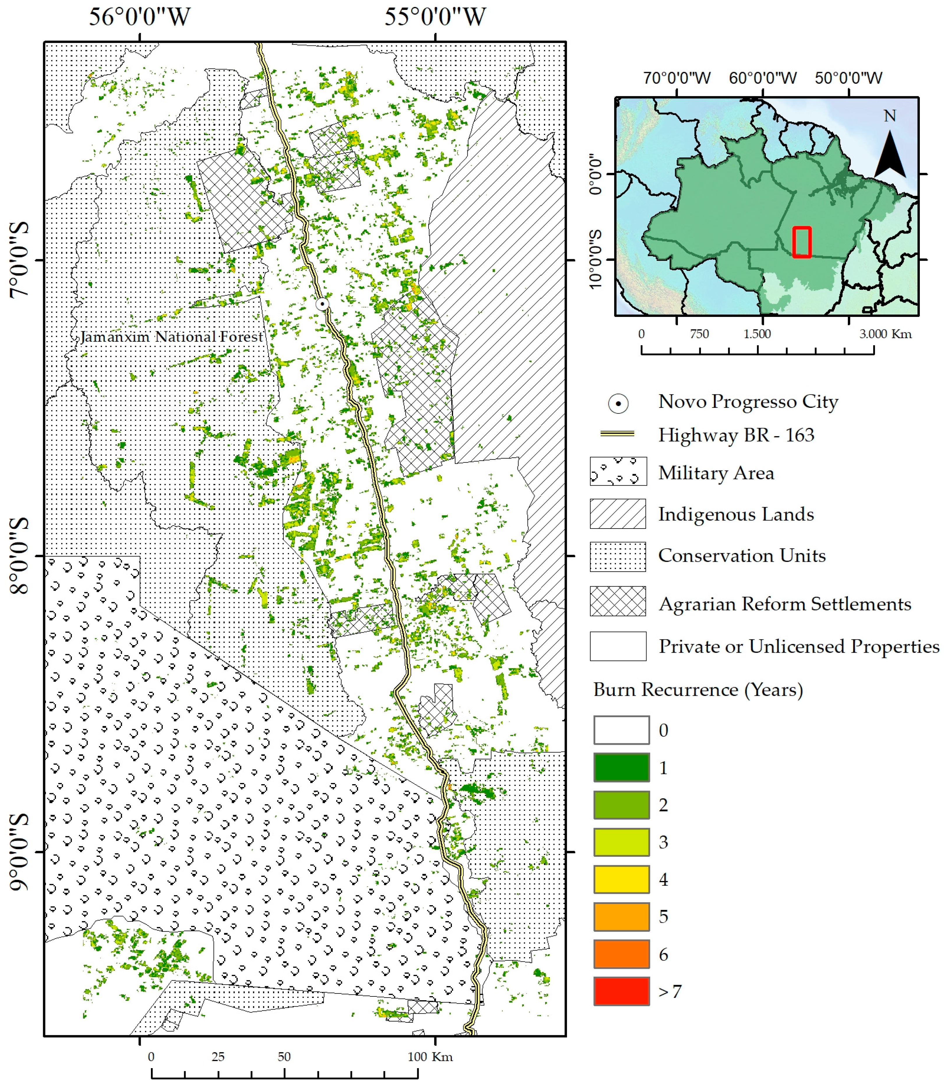
| Distance | 20 km | 40 km | 60 km | 80 km | 100 km | 120 km | 140 km | 160 km |
| Burned Area (%) | 12.5% | 10.1% | 3.7% | 1.6% | 0.9% | 2.7% | 2.5% | 0.7% |
© 2018 by the authors. Licensee MDPI, Basel, Switzerland. This article is an open access article distributed under the terms and conditions of the Creative Commons Attribution (CC BY) license (http://creativecommons.org/licenses/by/4.0/).
Share and Cite
Santana, N.C.; De Carvalho Júnior, O.A.; Gomes, R.A.T.; Guimarães, R.F. Burned-Area Detection in Amazonian Environments Using Standardized Time Series Per Pixel in MODIS Data. Remote Sens. 2018, 10, 1904. https://doi.org/10.3390/rs10121904
Santana NC, De Carvalho Júnior OA, Gomes RAT, Guimarães RF. Burned-Area Detection in Amazonian Environments Using Standardized Time Series Per Pixel in MODIS Data. Remote Sensing. 2018; 10(12):1904. https://doi.org/10.3390/rs10121904
Chicago/Turabian StyleSantana, Níckolas Castro, Osmar Abílio De Carvalho Júnior, Roberto Arnaldo Trancoso Gomes, and Renato Fontes Guimarães. 2018. "Burned-Area Detection in Amazonian Environments Using Standardized Time Series Per Pixel in MODIS Data" Remote Sensing 10, no. 12: 1904. https://doi.org/10.3390/rs10121904