An Unsupervised Classification Algorithm for Multi-Temporal Irrigated Area Mapping in Central Asia


1
Hydrosolutions Ltd., 8006 Zurich, Switzerland
2
Department of Engineering, University of Cambridge, Cambridge CB2 1PZ, UK
*
Author to whom correspondence should be addressed.
Remote Sens. 2018, 10(11), 1823; https://doi.org/10.3390/rs10111823
Submission received: 19 October 2018
/
Revised: 12 November 2018
/
Accepted: 14 November 2018
/
Published: 17 November 2018
(This article belongs to the Section Remote Sensing in Agriculture and Vegetation)
Abstract
:Sound water resources planning and management requires adequate data with sufficient spatial and temporal resolution. This is especially true in the context of irrigated agriculture, which is one of the main consumptive users of the world’s freshwater resources. Existing remote sensing methods for the management of irrigated agricultural systems are often based on empirical cropland data that are difficult to obtain, and that put into question the transferability of mapping algorithms in space and time. Here we implement an automatic irrigation mapping procedure in Google Earth Engine that uses surface reflectance satellite imagery from different sensors. The method is based on unsupervised training of a pixel-by-pixel classification algorithm within image regions identified through unsupervised object-based segmentation, followed by multi-temporal image analysis to distinguish productive irrigated fields from non-productive and non-irrigated areas. Ground-based data are not required. The final output of the mapping algorithm are monthly and annual irrigation maps (30 m resolution). The novel method is applied to the Central Asian Chu and Talas River Basins that are shared between upstream Kyrgyzstan and downstream Kazakhstan. We calculate the development of irrigated areas from 2000 to 2017 and assess the classification results in terms of robustness and accuracy. Based on seven available validation scenes (in total more than 2.5 million pixels) the classification accuracy is 77–96%. We show that on the Kyrgyz side of the Talas basin, the identified increasing trends over the years are highly significant (23% area increase between 2000 and 2017). In the Kazakh parts of the basins the irrigated acreages are relatively stable over time, but the average irrigation frequency within Soviet-era irrigation perimeters is very low, which points to a poor physical condition of the irrigation infrastructure and inadequate water supply.
1. Introduction
Globally, 60 to 70 percent of all withdrawals from freshwater resources are consumptively utilized in irrigation while irrigated agriculture produces 30 to 40 percent of the world’s food [1,2,3]. With continuing population growth and increased caloric intake of food, demand for irrigation water will rise over time [4]. To meet this demand in the future, sound water resources planning and management is imperative. These tasks require adequate data with sufficient spatial and temporal resolution. However, ground-based information on acreages of irrigated land is scarce and often unreliable, while the adoption of remote sensing technology in the planning and operational management of irrigated agricultural systems still represents a challenge [5]. Existing cropland mapping algorithms usually require detailed reference cropland layers (e.g., [6,7,8]), large number of sample training points (e.g., [9,10]) or empirical look-up tables (e.g., [11,12]) to build rule-based classifiers. The transferability in time and space of these supervised classification methods is therefore not always guaranteed.
The overarching goal of this research is to design an irrigation area mapping method that is convenient for local stakeholders who want to operationally produce high-resolution irrigation maps to assess water use and productivity, execute performance diagnosis and impact assessments, enable strategic planning or control water rights. One of the main requirements is that the classification algorithm is ready-to-use, i.e., the method should not depend on ground reference observations. To automatically classify without relying on pre-defined training data an unsupervised classification method is required. Indeed, unsupervised classification has been widely used for irrigated area mapping (e.g., [13,14,15]), although never in fully automated schemes. Unsupervised classification is often used to capture the full range of land use signatures over areas with wide and unknown ranges of vegetation types [14,15]. However, it is hard to control the number of classes when the method is used to classify heterogeneous landscapes. The application of unsupervised classification thus often requires a rigorous class identification and manual labeling process to group different classes. This combining of cover types is often strongly affected by subjective factors [16].
To prevent subjective decisions and to automate the irrigated area mapping algorithm we propose here a new integrated method of object-based segmentation in combination with pixel-based classification. Satellite images can be processed by image segmentation algorithms to identify homogeneous landscape units (e.g., [17]). Some earlier studies have used image segmentation to post-process per-pixel classifications [18,19]. Here we use image segmentation prior to per-pixel classification, for the purpose of automatically selecting suitable domains for unsupervised learning. Irrigation schemes in arid or semi-arid areas are easy to distinguish from the surrounding landscape due to the greenness of the surface in contrast to the dry surrounding area, especially during the late summer months. We therefore use a region growing clustering technique to identify large irrigation schemes. Such clusters of relatively homogeneous land cover are then used as training domains, where the unsupervised classification algorithm deals with finding a structure in the unlabeled data. Since irrigated agriculture is the main land use within the training regions, an unsupervised classification algorithm can be trained to partition image pixels into just two classes: a non-vegetated land use class and a vegetated land use class that includes irrigated areas.
One challenge in mapping irrigated croplands is the spectral similarity with wetlands or other natural vegetation [20]. Multi-temporal data analysis has proven to be very useful to distinguish irrigated areas from non-irrigated areas (e.g., [20,21,22]). Data from multiple time periods can trace the characteristic spectral response of crops according to their phenological evolution. The rationale of the multi-step mapping procedure proposed in this study is thus to first map vegetated areas on a monthly basis and then to make use of multi-temporal data to identify irrigated areas.
The entire irrigation mapping procedure is deployed on the Google Earth Engine (GEE) cloud computing platform [23], which offers the possibility to use and combine computationally expensive methods without the need for personal computational hardware and software. The ready-to-use availability of information from multiple sources in GEE allows to perform a multi-source data analysis, which in this study is used to fill data gaps and to reduce the uncertainty associated with the data from individual sensors [20]. Furthermore, ancillary information available trough GEE such as climate, topography or wetland inventories are used to improve classification accuracy or to assist with the interpretation of the results.
The method that we propose here combines, in a novel way, different image processing and statistical approaches and makes optimal use of the new possibilities offered by GEE. Objective measures of irrigated crop acreage are provided at different spatial (local to basin scale) and temporal scales (monthly to annual). Through an application of the method that focuses on the temporal evolution of irrigated areas (years 2000–2017) in the Chu and Talas River Basins in Central Asia, we show how remotely sensed high-resolution, multi-temporal information on irrigated land cover can support water planners and managers in a specific and targeted manner.
2. Study Site
Large scale irrigation systems in Central Asia cover more than 14 million hectares of land [24]. Snow- and glacier-melt fed rivers, most of them transboundary, feed into a vast and complex network of irrigation and drainage infrastructure which in many instances is also shared among the Central Asian Republics.
The two neighbouring Chu and Talas river basins are shared between upstream Kyrgyzstan and downstream Kazakhstan (Figure 1). The total area of the Chu River basin is approximately 62,500 km including 26,600 km (42.5 percent) in Kyrgyzstan and 35,900 km (57.5 percent) in Kazakhstan. Compared to this, the total area of the Talas River Basin is approximately 52,700 km, including 11,430 km (21.7 percent) in Kyrgyzstan and 41,270 km (78.3 percent) in Kazakhstan.
Both the Talas and the Chu Rivers are entirely endorheic. After draining the surrounding Tien Shan mountain ranges, the rivers run northwards and end in the Kazakh steppe without reaching the Syr Darya River that feeds the Aral Sea. The Talas River is 661 km long while Chu River has a length of 1067 km, approximately. The flow of both rivers is highly seasonal with spring and summer snow melt and—to a much lesser extent—glacier melt being the dominant runoff generation processes. The climate in Central Asia is continental and semi-arid with short, hot summers and long, cold winters [25]. Average monthly precipitation in the Talas River Basin ranges from 6 mm in August up to 50 mm in April while it ranges from 13 mm in August to 63 mm in April in the Chu River Basin [26]. Annual precipitation ranges usually between 300 and 500 mm in both basins.
During the Soviet era, reservoirs were built in the catchments to regulate the availability of irrigation water in the downstream. The Kirov reservoir in the Talas river catchment started operation in 1976. Its design capacity is 0.55 km3 [27]. In the Chu River Basin, there are two reservoirs, the Orto-Tokoy Reservoir in Kyrgyzstan built in 1957 with a capacity of 0.47 km3 and the Tasotkel Reservoir built in 1981 in present-day Kazakhstan [28].
A substantial fraction of the approximately 2 million people living in the two catchments depends directly on agricultural sector outcomes. The availability of proper amounts of water for irrigation at the right time and location is crucial for the societies there and farmer livelihoods, because agriculture is entirely irrigated [29].
Several elements increase the spatio-temporal variability in natural vegetation cover and complicate thus the task of irrigated area mapping: short summer rains can lead to considerable vegetation response, spring vegetation can last until mid-summer in years with sufficient rainfall, natural vegetation types vary with altitude and different types of wetlands (along discharge canals, along rivers, within endorheic deltas or in groundwater upwelling zones) undergo different seasonal changes.
3. Data
3.1. Satellite Data
Multi-temporal high-resolution data from different sensors are applied to map irrigated area in the Chu-Talas River Basins. To map irrigation areas, we use surface reflectance of three spectral bands (red, near-infrared [NIR] and middle infrared [MIR]). Each source of remote-sensing data employed in this study is listed below. Further details about the different data sets are provided in Table 1.
- Landsat 7 imagery: Landsat 7 is in near-polar orbit with repeat cover every 16 days. The resolution of the imagery is 30 m per pixel for the bands used in this study. Data from the USGS Landsat 7 Collection are available in GEE for the period since 1 Jan 1999. However, due to the low number of scenes available for our study region from the year 1999 we only use Landsat 7 imagery from the year 2000 onward. A scan line corrector failure on Landsat 7 after 31 May 2003 causes around 22 percent of each scene to be lost after that date [30,31]. Most studies therefore use multiple images to fill in data gaps (e.g., [32]) or the data is fused with observations from other remote sensing systems [6,33].
- Landsat 8 imagery: The Landsat 8 satellite was launched on 11 February 2013 and images the entire Earth every 16 days in an 8-day offset from Landsat 7. The spatial resolution of the images is 30 m. Landsat 8 data has been used previously for detecting irrigation extent by Chen et al. [34].
- SENTINEL 2 imagery: Sentinel 2 is a high-resolution, multi-spectral imaging mission supporting Land Monitoring studies. Sentinel 2A was launched on 23 June 2015 and revisits our study region every 10 days. The spatial resolution of the imagery is 10 m (Red, NIR) and 20 m (MIR). Sentinel 2 data have been used previously for mapping croplands by Belgiu and Csillik [35].
- MODIS Terra and MODIS Aqua imagery: The two MODIS satellites image the entire Earth every 1 to 2 days. We use the 8-day composite MODIS Surface Reflectance products available in GEE. Surface spectral reflectance of bands 1 (Red) and 2 (NIR) are available at 250 m resolution (MOD09Q1 and MYD09Q1 products) and the MOD09A1 and the MYD09A1 products provide the surface spectral reflectance of band 7 (MIR) at 500m resolution. The MOD09A1 and the MYD09A1 file include quality control flags for clouds that are used to mask clouds in each MODIS tile. MODIS Terra data are available for our study region for the time since the year 2000, and MODIS Aqua data since the year 2003. MODIS surface reflectance data have been used abundantly for irrigation area mapping (e.g., [14,21,22,34,36]).
3.2. Other Data Sets
For the calculation of terrain slopes, a high quality digital terrain model was utilized, i.e., the Shuttle Radar Topography Mission (SRTM) digital elevation model (DEM) [37]. The SRTM DEM has a resolution of 30 m and has been processed to fill data voids [38]. The Chu and Talas river basins boundaries have been derived using the SRTM DEM and a DEM flow-path routing algorithm.
Precipitation data are utilized to investigate the relationship between rainfall amounts and irrigated areas. For this purpose, the Climate Hazards Group InfraRed Precipitation with Station data (CHIRPS, version 2.0 final) is used. It is a 30 year quasi-global rainfall dataset [26]. Spanning 50 deg. S to 50 deg. N, starting in 1981 to near-present, CHIRPS incorporates 0.05 degree resolution satellite imagery with in-situ station data to create gridded rainfall time series for trend analysis and seasonal drought monitoring.
The Zhambyl branch of the Republican State Enterprise ’KazVodKhoz’ provided annual acreages of irrigated areas on the Kazakh side of the Chu and Talas basins between 2010 and 2016 that are used for validation. All information concerning administrative shapes have been downloaded from the Global Database on Administrative Areas (available at gadm.org). GIS data on rivers, irrigation canals (major and minor), reservoirs and natural lakes in the two basins are provided by the Kyrgyz National Scientific Research Institute of Irrigation.
4. Methods
4.1. Method Overview
The methodology is presented in Figure 2. First, image segmentation with an unsupervised Region Growing Clustering Algorithm is used to identify large irrigation schemes on Landsat 8 scenes. The image regions associated with the irrigation schemes are later used for unsupervised training of the pixel classification algorithm. Second, greenest pixel composite images are computed for every source of remote sensing data and every month of the irrigation period (April to September). Third, two unique clusters of pixels are identified within the buffered image training regions based on two vegetation indices and k-means clustering. The buffers around the training regions are necessary to increase the portion of non-irrigated land inside the training domains, which guarantees that the unsupervised cluster algorithm identifies a vegetated and a non-vegetated land use class. The algorithm then associates all image pixels with one of the two clusters. The hereby obtained monthly vegetation maps from different sources of remote sensing data are then fused into multi-source monthly maps. In the fourth step, all pixels that appear as vegetated in at least one of the six individual monthly maps are again partitioned into one of two classes through k-means clustering. This time, the multi-monthly data on the Normalized Difference Vegetation Index (NDVI) is used for partitioning, with the goal to separate spring vegetation from vegetation that persists throughout the irrigation season. Fifth, the pixels associated with persisting vegetation are sampled from two designated areas: (i) the training regions as identified in Step 1 and (ii) known areas with wetlands. A random forest classifier is then applied to identify pixels associated with wetlands throughout the scene (based on monthly NDVI and monthly red and near-infrared spectral signatures from the period April to November). The output of Step 5 are annual and monthly irrigation maps. Sixth, the monthly irrigation maps are validated against hand-labeled image data. We use the validation data also to identify a suitable range of buffer widths. Finally, steps 2–5 are repeated to create annual maps of summer irrigated cropland for 18 independent years from 2000 until 2017.
4.2. Identification of Training Sites for Unsupervised Classification
The region growing algorithm available in GEE is used to automatically identify large irrigation schemes (50–7000 km) that are then used as domains for unsupervised training of the classification algorithm. This image segmentation tool partitions image data into disjoint groups or clusters that are homogeneous in spectral properties [39,40]. Depending on the image resolution, larger or smaller landscape entities can be identified [41]. With a coarse pixel resolution, the image clusters correspond to objects such as lakes, forests, wetlands or agricultural lands. To identify large irrigation schemes in the Chu-Talas basins we analyze a late-summer Landsat 8 greenest pixel RGB composite (considering the period 1 August to 30 September 2016) resampled to pixel resolutions of 400 m and 500 m, respectively. Because the region growing algorithm is sensitive to image resolution, we use two different resolutions and merge the resulting features at the end of the procedure, to make sure that the relevant objects are identified. To identify the segmented image objects that correspond to the irrigation schemes we apply a number of filters. First, slopes higher than 5 and above 2500 m are masked out, since they are considered as boundaries for irrigated regions (e.g., [12]). Second, all objects with a total area of less than 50 km are discarded. We then calculate the median hue and the standard deviation of hue for all remaining image objects. Hue is an objective measure of color [42]. Values between 105 and 125 correspond to a green surface color, and are reliable indicators of irrigated surfaces during the Central Asian summer (Supplementary Figure S1). Thus all objects with a median hue value outside this range are discarded, and also all objects with a standard deviation in hue higher than 15. As a last step we remove all features that intersect with features of the World Database on Protected Areas (WDPA). In the Chu-Talas Basins these features correspond to areas with wetlands that remain green throughout the summer (Figure 3).
The polygons that are obtained from the procedure enclose areas of relatively homogeneous irrigated agricultural land. However, the polygons must contain both irrigated and non-irrigated land cover, which the unsupervised per-pixel classification algorithm will be trained to differentiate in the next step. To increase the portion of non-irrigated land inside the training domains it might therefore be necessary to add buffers around the polygons identified through image segmentation. We therefore test buffer widths between 0 and 15,000 m (steps of 500 m) to identify a suitable range of buffer widths. For each buffer width, we calculate the resulting classification accuracy with respect to a validation data set available for the year 2016 (see Section 4.6). The analysis is performed separately for the training regions in the Chu and in the Talas Basin, respectively, to assess if ideal buffer widths are site dependent.
4.3. Monthly Vegetation Maps
To generate monthly vegetation maps, we apply two filters to spectrally transformed image data. The two proxies for vegetation variability that are considered in this step are: (i) NDVI and (ii) the Hue-Intensity (H-V, V=value) component. NDVI is derived from Red and the NIR spectral bands and has been closely related to plant moisture availability [43], leaf area index [44], primary production [45], or vegetation fraction [46] and is therefore almost indispensable for mapping vegetation [20]. NDVI changes over the growing season, and unsupervised cluster analysis is therefore useful to identify transient thresholds. H represents the spectral composition of the color in terms of red, yellow, green and others with values between 0 and 360. V is defined as the brightness of the color. To obtain values of H-V for each pixel, MIR, NIR, and Red values are assigned to red, green, and blue colors (RGB) and are transformed into the HSV color space [47]. The colorimetric properties of vegetated and non-vegetated land are well separated in the H–V space (Supplementary Figure S2), which makes it a suitable filter for vegetation mapping. Characteristic values of H-V for vegetated land are associated to bright and green colors.
An unsupervised cluster analysis is performed with each of the two vegetation indices extracted from monthly composite images (see Section 4.5). Only the pixels attributed both times to the cluster associated with vegetated land cover are classified as vegetated in the final monthly vegetation maps (Figure 4a). The algorithm that is used for unsupervised classification is the k-means cluster analysis algorithm [48,49]. Input for the k-means algorithm is the number of k clusters desired, which in our case is two. The algorithm is trained with 1000 pixels sampled randomly from within the training regions, and then partitions all image pixels into one of the two clusters. The vegetated land use class is always assigned to the cluster with the higher mean NDVI, and the non-vegetated class is assigned to the second cluster.
4.4. Multi-Temporal Analysis
4.4.1. NDVI Time-Series
NDVI time series are often used for the classification of different crops, as they reflect characteristic vegetation growth processes by usually continuous and smooth curves (e.g., [16]). Here, we use time series of monthly NDVI to distinguish temporary spring vegetation from irrigated crops and other persisting vegetation. What distinguishes natural spring vegetation from irrigated land is a decrease in NDVI over the summer period due to differences in soil moisture supply. We therefore use the monthly vegetation maps to perform again a k-means cluster analysis restricted to a 2-cluster solution. Observations are not sampled from within the training regions, but from any pixel that has been classified as vegetated in any of the monthly maps from April to September (Figure 4b). The unlabeled input training data for the k-means algorithm are the April to September monthly NDVI values of each sampled pixel. The assumption is that a large fraction of these pixels represents spring vegetation. The cluster analysis will therefore identify two main land cover classes: one cluster with persisting vegetation with a high NDVI throughout the season, and one cluster with high values of NDVI only in spring/early summer. The persisting vegetation class label is therefore always automatically assigned to the cluster with the higher mean September NDVI.
Pixels with a slope higher than 5 or an elevation higher than 2500 m are not considered by the multi-temporal NDVI analysis. The corresponding pixels are classified as non-irrigated in all monthly or annual maps. Equally, we filter out pixels of the persisting vegetation map that are inconsistently classified as vegetated less than twice in the July, August and September vegetation maps (Figure 4b).
4.4.2. Summer Vegetation Filter
The similarity of spectral behavior of natural summer vegetation and irrigated agricultural land often leads to misclassifications [3,50]. Such natural vegetation appears in the vicinity of water courses/bodies or where groundwater provides sufficient moisture. However, it is possible to identify wetlands by low near-infrared and low red reflectivity [15,20]. Natural vegetation response can also be distinguished from irrigated area by the absence of drops in NDVI due to crop harvest [51]. However, natural summer vegetation essentially depends on rainfall amounts, which are subjected to considerable inter-annual variability. In dry years, pixel misclassifications due to green summer vegetation may be negligible. Unsupervised classification is therefore not an ideal instrument to reliably detect such areas. We therefore choose a different approach that is based on the Random Forest (RF) algorithm. RF is a supervised classification algorithm that belongs to the family of decision trees and has been commonly applied for land cover classification [52].
Supervised classification requires a training data set. However, no prior information on the exact location of training pixels (‘irrigated’ or ‘natural’) is required here. It is sufficient to roughly outline areas with natural vegetation response (called ‘Wetland’ training regions in Figure 3). The algorithm then samples from the annual map generated in the previous step pixels with persisting summer vegetation: if they are sampled from within wetland image regions, they are automatically labeled as ‘natural’, and if they are sampled from within the irrigated training regions (Figure 3), they are labeled as ‘irrigated’. It is possible to use WDPA sites as training regions, assuming that irrigation activities are absent within nature conservation areas. In that case the sampling is fully automatic, since an updated global data set of WDPA polygons is available on GEE. WDPA sites are present within the Chu-Talas Basins (Figure 3), and we do use them as training polygons. However, the accuracy of RF classification increases if samples are available from various locations representing different types of natural vegetation. We therefore decided to consider also manually defined wetland training regions (Figure 3). In this way we make sure that the irrigated crop acreages calculated in this study represent the maximum accuracy that can be achieved with our method.
RF classification is used with the following set of predictors: (i) monthly NDVI from April to November, (ii) monthly values of NIR and (iii) monthly values of Red from April to November (in total 24 variables). Data from the months October and November are used because they represent the situation after harvest.
The RF algorithm depends only on two user-defined parameters: the number of trees and the number of random split variables [52]. Accuracy converges at around 100 trees, while it is recommended to keep the number of split variables small [52,53]. In this study we apply the RF algorithm with 100 trees and 1 variable per split. RF is not sensitive to noise or over-fitting [54]. If a few irrigated patches are present within the wetland training regions or if small wetlands exist within the irrigated training regions, this will not reduce the performance of the RF classifier and those areas will be classified correctly.
In the final annual irrigation map that results from this step, pixels associated with natural vegetation are classified as non-irrigated. To obtain final monthly irrigation maps, the monthly vegetation maps (Figure 4a) are post-processed with the annual irrigation map (pixels in the vegetation maps not classified as irrigated in the annual map are filtered out). With the area information of every pixel, the total monthly or annual irrigated areas can be calculated and compared with official statistics where available.
4.5. Compositing and Data Fusion
To reduce the effect of clouds as well for dealing with the scan line corrector failure on Landsat 7, greenest pixel composite images are computed for every month and every source of remote sensing data (Table 1). The composite for every pixel is created by choosing the pixel with the highest NDVI value over all available scenes [55]. The resulting composite image is a mosaic of those pixels with the highest amount of vegetation during that period, a so-called NDVI composite.
Because of the relatively long average revisit intervals of Landsat 7 and 8 satellites (16 days), only 2 to 4 images per month are available from those sensors for every location in our study region. We therefore fuse the monthly vegetation maps generated from data obtained from different sensors to fill data gaps (Section 4.3, Figure 4a). The different sources of satellite data used in this study are combined in three different ways: Landsat 7 data are combined with MODIS Terra and with MODIS Aqua data, respectively, to form two products called ‘L7/MOD’ and ‘L7/MYD’ irrigation maps hereafter, and the three high-resolution sensors Landsat 7, Landsat 8 and Sentinel 2 are combined to form the ‘L7/L8/S2’ product. The final irrigation maps have a resolution of 30 m, which is the native resolution of the Landsat 7 and 8 imagery (Table 1). To discuss the advantages of data fusion and high image resolution, we compare the accuracy of the L7/MOD and the L7/L8/S2 products to 250 m resolution irrigation maps composed only from MODIS Terra data.
We use the Sentinel 2 QA60 band, a bit-mask band containing cloud mask information, to filter out cloudy pixels in Sentinel 2 data [56]. For Landsat 7 and Landsat 8 data we calculate the cloud-likelihood score of each pixel using the GEE Landsat simpleCloudScore algorithm [57]. Pixels with a cloud score higher than 30% are masked out. The L7/L8/S2 product is formed by NDVI compositing of the monthly vegetation maps compiled for every sensor in Step 1 of the irrigated area mapping algorithm (Figure 4a).
In the L7/MOD and L7/MYD products Landsat 7 is given priority due to its higher spatial resolution. Only when pixels have a cloud score higher than 30% we use MODIS data for Step 1 of the irrigated area mapping procedure (Figure 4). In steps 2 and 3, however, we use only MODIS NDVI, red and NIR data, even if Landsat 7 data are available. The reason for this is that the fusion of spectral data between Landsat 7 and MODIS is not straightforward due to differences in spatial resolution, wavelengths and radiometric inconsistencies [33], which could create artifacts in the RF derived irrigation maps. Due to the higher resolution of Landsat 7 data it would be preferable to use only data from this sensor, which is however not possible for most years because of missing data, e.g., due to clouds in monthly Landsat 7 composites. For the L7/L8/S2 product we use fused image data from NDVI composite maps for RF classification.
4.6. Classification Validation
4.6.1. Generation of Hand-Labeled Validation Data
Image segmentation for object-based analysis is used in this study not only for the delineation of training domains, but also to identify a large number of image objects that are then hand-labeled by photo-interpretation to generate a validation data set. Again, we use the Region Growing tool in GEE for unsupervised image segmentation, but applied to different images than used for growing the training regions and with a higher pixel resolution. For this purpose we selected seven selected Landsat 8 scenes from six locations within the Chu-Talas Basins (Figure 3). The seven scenes reflect the different phenological stages of the crops during the 2016 irrigation season and the six locations take into account possible spatial variability of crop appearance within the Chu-Talas basins (e.g., due to different crop types) and the presence of natural vegetation such as wetlands. The images are resampled to 80 m pixel resolution. At this resolution, image segmentation selects cropland units or other physically meaningful landscape entities whose surface status (irrigated or non-irrigated) can be unambiguously determined. Through photo-interpretation and hand-labeling of the surface status of these entities, a data set is obtained that can be used for independent validation of the mapping algorithm. Objects where the surface status is not clear or which have an area below 2 ha are discarded from the validation data set.
4.6.2. Accuracy Assessment
The accuracy of monthly irrigation maps derived for the year 2016 is discussed in terms of percent agreement with our validation set of data. We calculate the fraction of correctly classified pixels in relation to the total number of available pixels across all validation scenes (named ‘overall accuracy’ hereafter). A confusion/error matrix approach is used to express producer’s accuracy (or omission error) and user’s accuracy (or commission error) [58,59]. Furthermore, the derived multi-annual irrigated areas are also validated against available official data (Section 3.2).
4.7. Analysis of Spatial and Temporal Trends
Using the annual irrigated acreages from the years 2000 until 2017, the non-parametric Sen’s slope estimator and corresponding confidence intervals are computed to detect whether there are significant trends in the development of irrigated areas over time. Sen’s slope is less sensitive to outliers than the common least squares estimate using linear regression [60]. To assess the controlling factors of inter-annual variations we calculate correlation coefficients between annual irrigated area and pre-season and in-season precipitation, respectively. In-season precipitation is cumulative precipitation from April 1 through September 30 whereas pre-season precipitation is cumulative precipitation from October 1 through March 31 prior to the irrigation season. The temporal trends and the correlation coefficients are calculated for each basin separately and also for the Kazakh and the Kyrgyz part of each basin. For the downstream Kazakh areas, we consider the precipitation over the entire basin to calculate correlation coefficients whereas annual irrigated areas of the upstream Kyrgyz part are related to precipitation over the Kyrgyz part only.
To analyze spatial patterns, the frequency of irrigation occurrence as well as the irrigation change intensity is calculated for every pixel within the study area (e.g., [9]). The irrigation change intensity indicates where irrigation occurrence increased, decreased or remained invariant over time. To calculate the change intensity, the irrigation frequency of the first five years of the study period is subtracted from the irrigation frequency of the last five years.
5. Results
5.1. Accuracy and Uncertainty Assessment of Classification Results
5.1.1. Validation Against Hand-Labeled Data
The validation data set generated through image segmentation and hand-labeling consists of 11,501 objects with a total area of approximately 1961 km. This corresponds to more than 2.5 million pixels at the resolution of Landsat 8 data that can be used for the accuracy assessment of the classification results, whereas each of the seven scenes includes at least 200,000 pixels. The fraction of irrigated pixels is 30% and depending on the scene varies between 9.2% and 50.2%.
If buffers are added around training sites in the Chu basin, the overall classification accuracy increases by up to 2% (Figure 5a). Buffers around training regions in the Talas basin increase the classification accuracy by up to 1%. The effect is relevant for the producer’s accuracy, which increases by up to 10% (Figure 5c), while the user’s accuracy is again relatively insensitive to buffer widths (Figure 5b). Larger training regions with larger fractions of non-irrigated areas decrease the risk of dividing areas that are actually irrigated into different clusters. Consequently, if buffers are used, the total number of pixels that are classified as irrigated increases. However, if the buffer widths are too large, too many pixels are classified as irrigated and the Producer’s Accuracy decreases again. The maximum overall and Producer’s accuracy are achieved with buffer widths of approximately 4000 m, both in the Chu and in the Talas Basins. This result is not affected by the spatial proximity between training regions and validation data, as the same pattern emerges if the two spatial datasets are strictly separated between the two basins (Supplementary Figure S4). In the following, we consider therefore buffers between 2000 m and 6000 m for all subsequent applications of the unsupervised learning algorithm. The range of values allows to provide an estimate about the uncertainty in total irrigated areas.
The accuracy indicators are consistently higher if training regions within the Chu basin are used for irrigation detection (Figure 5). Most likely this is because a majority of the available validation data (67% of the total validation data area) are available within or in close vicinity to the training regions in the Chu basin. Figure 6a confirms that the overall accuracy is 2–4% higher if the training regions are located in the same basin as the validation data. We conclude from this that it is beneficial for the classification accuracy to train the algorithm locally. In the following, the calculations concerning the Chu or the Talas basin, respectively, are therefore always performed separately.
The performance of the L7/MOD and the L7/L8/S2 products does not differ significantly. For both multi-sensor products, we calculate an overall accuracy between 87.5% and 88.5%. The median User’s and Producer’s accuracy of the two products differs by less than 1.5%. In contrast, for the 250 m resolution MODIS Terra irrigation maps we calculate overall accuracies of about 85%. The median User’s and Producer’s accuracies of the MODIS maps are 4–6% lower than their equivalents for the L7/MOD and L7/L8/S2 products (Figure 6a).
For individual scenes the fraction of correctly classified pixels varies between 77% and 96% (Figure 6b). The highest accuracy is achieved in Area I, which is located in the Kazakh lowlands of the Talas Basin (Figure 3). For MOD monthly irrigation maps we calculate accuracies that are generally 2–7% lower than those of the L7/MOD and L7/L8/S2 products (Figure 6b), except in Area I, where the MOD product performs about as well as the two higher resolution products.
All irrigated area mapping products provide very accurate estimates of total irrigated areas in comparison to the validation data. The coefficient of determination (R) between irrigated pixel numbers in the validation data and in the monthly irrigation maps varies between 0.96 and 0.99 (Figure 6c). The total number of pixels classified as irrigated across all 7 validation scenes differs only by −0.5% and by +1.7% in the case of the L7/MOD and the L7/L8/S2 monthly irrigation maps, respectively. The MOD monthly irrigation maps overestimate the total number of irrigated pixels by 3.5%.
All three processing steps (Figure 4) are necessary to obtain a good agreement between total irrigated areas of the L7/MOD product and the validation data (Figure 7). The total number of irrigated pixels is still overestimated by 40% after Step 1. The overall accuracy increases between Step 1 and Step 3 from 84.0 ± 0.5% to 88.1 ± 0.5%. Steps 2 and 3 cause an increase of the user’s accuracy by about 14% each, on the expense of an equal decrease in the Producer’s accuracy (Figure 7b). The error of omission and the error of commission are approximately of similar magnitude in the final maps, which means that the area missed by the classification is the same as the area which is erroneously included. Consequently, these two errors cancel each other out.
The benefit of each processing step on classification accuracy differs for irrigation maps associated to different months and locations (Figure 7c). The consideration of NDVI time-series to characterize irrigated pixels (Step 2) increases the classification accuracy of the April irrigation map by 12%. Other scenes do not benefit from this step and the classification accuracy does not increase. Step 2 is therefore only necessary to obtain monthly maps for the very early irrigation season, when spring vegetation is still present (Supplementary Figures S5 and S6). Consequently, the clustering of NDVI time-series has also no effect on the the annual irrigation maps, because April to June maps are not required to compose annual irrigation maps. In the following, Step 2 is therefore skipped for the determination of annual irrigated areas (but the consistency check with July to September vegetation maps is still performed, see Section 4.4.1 and Figure 4b). Step 3 of the irrigation methodology increases the classification accuracy within Area I by 6% (Figure 7c), where large wetlands are present (Figure 3). At other locations Step 3 has only a minor or insignificant effect on irrigation classification accuracy.
5.1.2. Uncertainty and Accuracy of Multi-Annual Irrigated Areas
Uncertain buffer widths between 2000 m and 6000 m around training features identified through image segmentation lead to average uncertainties in multi-annual irrigated areas of 1.4–4.5% (Table 2). The root mean square deviations between irrigated areas derived from the L7/MOD product and the L7/MYD and L7/L8/S2 products are between 1.5–8.2%, except for the Kazakh part of the Talas Basin where the root mean square error (RMSE) between the L7/L8/S2 product and the L7/MOD product is 15.2%. The latter value is similar to the RMSE between KazVodKhoz data and the L7/MOD irrigated areas (16.0%, Table 2).
At the Kazakh side of the Chu basin the determined annual irrigated areas are in general very consistent with available KazVodKhoz data (Figure 8). The RMSE between the two datasets for the period 2010–2015 is 47 km, which represents about 5% of the annual irrigated areas (Table 2). However, the error is much larger for the year 2016, where the calculated acreages overestimate the reference data by 365 km or 59%.
5.2. Classification of Irrigated Areas
Using the boundaries of the administrative divisions, we calculate the development of irrigated areas at national levels (Figure 8 and Figure 9). Over the assessment period, the mean irrigated area in the Talas Basin is 2038 km and 3840 km in the Chu Basin, respectively (Table 3).
For the Kyrgyz part of the Talas basin, we identify a robust increasing trend in irrigated areas over time that is highly significant (at the 0.001 level, see Table 3). The trend indicates that since the year 2000, irrigated areas are on average increasing by 14.5 km per year, which corresponds to a total increase in irrigated areas by 23% between the years 2000 and 2017. At national levels of the Chu basin, the annual irrigated areas seem to have remained approximately constant since the year 2000 (Figure 8 and Figure 9). In the Kazakh part of the Talas basin, irrigated areas might even have decreased by about 12.3% according to the calculated Sen’s Slope, but the trend is not significant (Table 3).
The data for the Kyrgyz side of the Chu River Basin and the Kazakh side of the Talas river basin show significant inter-annual variability in the development of the irrigated areas (Figure 8 and Figure 9). The variations amount to up to ±20% of the mean annual irrigated area. For the Kyrgyz part of the Chu basin, we calculate a correlation coefficient of 0.67 between in-season precipitation and irrigated acreages (Table 3). The inter-annual variability is therefore due to higher than average acreages of irrigated area in particularly wet years (i.e., the years 2002, 2003, 2009 and 2016, see Figure 8).
6. Discussion
6.1. Uncertainty and Accuracy Assessment
Wegerich [61] states that in 2008 there was 1149 km of irrigated land in the Talas River Basin in Kyrgyzstan and 793 km in Kazakhstan. Kireycheva et al. [62] write that there are 1150 km irrigated in Kyrgyzstan and 630 km in Kazakhstan. For 2008, our L7/MOD classification results are 1230 km of irrigated land in Kyrgyzstan and 810 km in Kazakhstan. The results of the classification for 2015 are 1330 km on the Kyrgyz part of the basin and 720 km on the Kazakh part. Our numbers therefore coincide well with the estimates of Wegerich [61] (differences of only 2–7%). The difference with respect to Kireycheva et al. [62] is higher (14.3–15.6%). However, the value of Kireycheva et al. [62] for the Kyrgyz part is almost identical to the value of Wegerich [61], whereas our multi-annual analysis shows clearly that irrigated areas in the Kyrgyz part of the Talas basin are increasing over time (Table 3).
For the Kyrgyz parts of the basins our uncertainty estimates (Table 2), our validation data and the available literature data attest a very high accuracy of less than 3% to our annual irrigation area estimates. The uncertainties are higher in the Kazakh parts of the basins (up to 16.9%, see Table 2). The Kazakh parts are characterized by low-lying steppe lands with inland river deltas and wetlands, where strongly varying precipitation amounts can lead to vegetation responses over large swaths of normally dry land. A NDVI composite naturally picks up this vegetation response which can lead to misclassifications and uncertainties, in spite of the natural vegetation filters applied in this work. This points to an important limitation of the irrigated area mapping approach presented here. The accuracy of our approach decreases in regions with sufficient rainfall or soil moisture to sustain natural vegetation during summer.
Our calculated acreages overestimate the Chu KazVodKhoz reference data available for the year 2016 by 365 km or 59% (Figure 8). The KazVodKhoz data of that year report a total irrigated area that is 268 km lower than the average 2010–2015 of the same data set (Figure 8). It is unlikely that also the cultivated area dropped by the same value, since 2016 was a water rich year. Furthermore, 2016 is also the year for which a validation set of data is available, and no significant overestimation of mapped irrigation areas has been identified (Section 5.1). Rainfed agriculture can be excluded as a possibility, since in-season precipitation at the Kazakh side was less than 200 mm (Figure 8), whereas the crop water demand is at least 800 mm [63]. The discrepancy with KazVodKhoz data for the Chu Basin in 2016 does therefore not point to a an error in our remotely sensed estimates of irrigation areas but rather to an artifact in the reference data.
6.2. Monitoring of Agricultural Systems
Figure 10 shows the frequency of irrigation occurrence between 2000 and 2017 for each 30 m grid cell in the upper Chu and Talas basins. The canal infrastructure nicely outlines the irrigated perimeters (Figure 10). The irrigation canal infrastructure in the Chu-Talas basins dates back to the Soviet era and, according to local stakeholders, no significant new extensions of irrigated perimeters were realized during the time horizon under consideration. The post-Soviet transition period in the last decade of the twentieth century was a time of severe struggle in the irrigation water sector [29]. The detected irrigation area increase in some parts of the basins therefore reflects the gradual rehabilitation of the existing systems. In the Kazakh parts of the Chu-Talas basins, however, irrigated acreages have been relatively constant over the last 18 years (Table 3). Wegerich [61] states that in earlier times, the total irrigated land in the Kazakh part of the Talas basin was almost equal to the irrigated area in the Kyrgyz part. Nowadays, according to our calculations, the irrigation extent between 2000 and 2017 in the Kyrgyz part is on average 1.5 times larger as compared to the Kazakh part of the Talas basin. Figure 10a confirms that only a small part of the Soviet canal infrastructure is in use on the Kazakh side of the border in the Chu Basin.
Significant correlations between in-season precipitation and irrigated acreages (Table 3) point to inadequate access to water storage, which limits irrigation expansion in dry years. The irrigation perimeters above the main canals have only access to water from small streams that run from the Tien Shan mountains, which provide more water in wet years. The lower lying parts of the basins have access to reservoir storage, and consequently the correlations between in-season precipitation and irrigated acreages are lower (Table 3).
With the derived multi-year high resolution data, monitoring of irrigated areas can be carried out from the transboundary level down to the level of Water User Associations (WUAs). We demonstrate the potential of the derived irrigation data for monitoring of irrigated agricultural systems by the example of three WUAs within the Kyrgyz part of the Chu-Talas basins: WUA Jorgo in the Talas Basin and WUA Uzun Kyr and WUA El Suu in the Chu Basin (Figure 1 and Figure 11).
Figure 12 shows the annual acreages of irrigated area within the WUA units. In WUA Jorgo the total irrigated area increased from 2000 until 2007 by 35%, but have been constant since then. In Uzun Kyr, irrigated acreages have been relatively stable since 2003. Also the wet years 2009 and 2016 are not characterized by higher than usual monthly irrigated areas (Figure 12). In contrast, the areas that have been irrigated in WUA El Suu in 2016 are 45% larger than in any other year. This WUA is located at the tail end of the Big West Chu Canal and suffers from inadequate and highly erratic water supplies from the canal. Consequently, a majority of WUA El Suu units are not cultivated in normal years (Figure 11b). Uzun Kyr, on the other hand, is located near the intake of the West Big Chu Canal. The available water is sufficient to irrigate all of its area (Figure 11a) due to its favorable upstream position along the main canal. Similarly, WUA Jorgo is located immediately downstream of Kirov Reservoir in the Talas River Basin and the Canal supplying the WUA is providing sufficient irrigation water with great reliability.
The analysis of the change in irrigation intensity provides a powerful approach to assess local conditions at WUA levels (Figure 11). Both the direction of change (i.e., increase, decrease or no change) and its intensity are documented. For example, the positive irrigation changes just outside the WUA units in WUA Jorgo (Figure 11c) are due to the rehabilitation of a pump-irrigation system that was abandoned after the fall of the Soviet Union (source: WUA management, personal communication). The negative changes in irrigation intensity, on the other hand, demonstrate the growth of villages (e.g., WUA Uzun Kyr, south central and central parts) or help to identify the deterioration of land melioration conditions, e.g., due to salinization of fields (e.g., WUA Jorgo, center). Remotely sensed products such as the one presented here can help in the reclamation of affected land and be used for consistent monitoring.
7. Conclusions
This paper presents a new approach for multi-temporal, high-resolution irrigated area mapping using remotely sensed imagery. The approach combines in a novel way unsupervised image segmentation, unsupervised pixel classification and multi-temporal image analysis. The combination of these techniques enables the detection of irrigated areas without requiring any reference cropland data for training of the mapping algorithm. The mapping algorithm is entirely implemented in Google Earth Engine, with the advantage that the processing of the data does not require local infrastructure apart from an ordinary personal computer and access to internet. In combination with ancillary information available in Google Earth Engine the procedure is fully automatic and generates monthly and annual irrigated area maps with a 30 m resolution.
The algorithm is applied in the Chu-Talas River Basins in Central Asia, shared between upstream Kyrgyzstan and downstream Kazakhstan, where we produce irrigated area maps for 18 independent years from 2000–2017. Our validation data set is a hand-labeled library of 11,501 landscape objects, representing more than 2.5 million pixels at 30 m resolution. The different multi-source irrigation maps assessed in this study achieve classification accuracies that vary between 77% and 96% for individual scenes. Considering all available validation data across different scenes, the accuracy is 87–89% and the total mapped irrigated area differs by less than ±2%. Based on the available reference data, data from the literature and based on a multi-source data analysis, the average uncertainty of multi-annual irrigated acreages can be estimated to less than 5% in the Kyrgyz part of the Chu-Talas Basins. The uncertainty estimates for the Kazakh parts are higher (5–15%) due to mis-classifications in inland river deltas and wetlands. In summary, our accuracy assessment shows that the classification produces robust, reliable and reproducible results.
The scalable outputs of the irrigated area mapping algorithm can help local stakeholders to study the performance of vast and complex irrigation systems in great detail and help in monitoring irrigation activities at the field scales up to the transboundary levels. Our main finding is that irrigated area development in the Chu-Talas basins follows distinct patterns in different parts of the basins. In the Kazakh parts of the basins the irrigated acreages are relatively stable over time, but we show that the capacity of the Soviet-era irrigation system that is still in place is not fully exploited. In the Kyrgyz part of the Talas Basin, on the other hand, the irrigated areas have increased by 23% in the last 18 years within the Sovjet-era irrigation perimeters, which reflects the gradual rehabilitation of the existing systems after the difficult post-Soviet transition period.
Due to the similarities in climate, our approach can be used for the large-scale monitoring of summer irrigation activities throughout Inner Asia (https://code.earthengine.google.com/a8623e7373e54c27e643f021c0445984). A next step will be to operationalise this product for the concurrent monitoring of in-season irrigation activities. This will help local authorities to monitor irrigation system performance and irrigation activities over time with high precision and in the absence of reliable ground-based data.
References
Supplementary Materials
The following are available online at https://www.mdpi.com/2072-4292/10/11/1823/s1.
Author Contributions
S.R. designed and proposed the main structure of this research, analyzed the data and wrote the manuscript. T.S. organized and supervised the research and developed this study together with S.R. and T.H. All authors discussed and reviewed the manuscript.
Funding
This study was partially funded by the Swiss Agency for Development and Cooperation (Projects No. 7F-09408.01.03 and No. 7F-09680.01.02).
Acknowledgments
We thank the Department of Water Resources and Melioration, Ministry of Agriculture in the Republic of Kyrgyzstan for general support of this work. We thank the Chu-Talas Transboundary River Commission and the International Water Management Institute in Tashkent, Uzbekistan as well as the Djambil Branch of the RGP Kazkodkhoz in Kazakhstan for the provision of agricultural statistics data. Furthermore, we are grateful for the provision of geospatial data by the GIS and Database Laboratory at the Kyrgyz National Scientific Research Institute of Irrigation as well as for critical feedback from Lubov Gerashenko. We also acknowledge helpful in-depth discussions with Vitaly Shablowski and Eva Polyak at this institution. Without the help and input from the numerous local stakeholders, this research work would not have been possible.
Conflicts of Interest
The authors declare no conflict of interest.
References
- Bastiaanssen, W.G.M.; Molden, D.J.; Makin, I.W. Remote sensing for irrigated agriculture: Examples from research and possible applications. Agric. Water Manag. 2000, 46, 137–155. [Google Scholar] [CrossRef]
- Seckler, D.W. World Water Demand and Supply, 1990 to 2025: Scenarios and Issues; IWMI: Colombo, Sri Lanka, 1998; Volume 19. [Google Scholar]
- Thenkabail, P.S.; Schull, M.; Turral, H. Ganges and Indus river basin land use/land cover (LULC) and irrigated area mapping using continuous streams of MODIS data. Remote Sens. Environ. 2005, 95, 317–341. [Google Scholar] [CrossRef]
- Bruinsma, J. World Agriculture: Towards 2015/2030: An FAO Perspective; Earthscan: London, UK, 2003; p. 432. [Google Scholar]
- Meier, J.; Zabel, F.; Mauser, W. A global approach to estimate irrigated areas—A comparison between different data and statistics. Hydrol. Earth Syst. Sci. 2018, 22, 1119–1133. [Google Scholar] [CrossRef]
- Thenkabail, P.S.; Wu, Z. An automated cropland classification algorithm (ACCA) for Tajikistan by combining landsat, MODIS, and secondary data. Remote Sens. 2012, 4, 2890–2918. [Google Scholar] [CrossRef]
- Xiong, J.; Thenkabail, P.S.; Gumma, M.K.; Teluguntla, P.; Poehnelt, J.; Congalton, R.G.; Yadav, K.; Thau, D. Automated cropland mapping of continental Africa using Google Earth Engine cloud computing. ISPRS J. Photogramm. Remote Sens. 2017, 126, 225–244. [Google Scholar] [CrossRef]
- Gao, Q.; Zribi, M.; Escorihuela, M.; Baghdadi, N.; Segui, P. Irrigation Mapping Using Sentinel-1 Time Series at Field Scale. Remote Sens. 2018, 10, 1495. [Google Scholar] [CrossRef]
- Estel, S.; Kuemmerle, T.; Alcántara, C.; Levers, C.; Prishchepov, A.; Hostert, P. Mapping farmland abandonment and recultivation across Europe using MODIS NDVI time series. Remote Sens. Environ. 2015, 163, 312–325. [Google Scholar] [CrossRef]
- Sharma, A.K.; Hubert-Moy, L.; Buvaneshwari, S.; Sekhar, M.; Ruiz, L.; Bandyopadhyay, S.; Corgne, S. Irrigation history estimation using multitemporal landsat satellite images: Application to an intensive groundwater irrigated agricultural watershed in India. Remote Sens. 2018, 10. [Google Scholar] [CrossRef]
- Ambika, A.K.; Wardlow, B.; Mishra, V. Remotely sensed high resolution irrigated area mapping in India for 2000 to 2015. Sci. Data 2016, 3, 1–14. [Google Scholar] [CrossRef] [PubMed]
- Conrad, C.; Schönbrodt-Stitt, S.; Löw, F.; Sorokin, D.; Paeth, H. Cropping intensity in the Aral Sea Basin and its dependency from the runoffformation 2000–2012. Remote Sens. 2016, 8. [Google Scholar] [CrossRef]
- Alexandridis, T.K.; Zalidis, G.C.; Silleos, N.G. Mapping irrigated area in Mediterranean basins using low cost satellite Earth Observation. Comput. Electron. Agric. 2008, 64, 93–103. [Google Scholar] [CrossRef]
- Biggs, T.W.; Thenkabail, P.S.; Gumma, M.K.; Scott, C.A.; Parthasaradhi, G.R.; Turral, H.N. Irrigated area mapping in heterogeneous landscapes with MODIS time series, ground truth and census data, Krishna Basin, India. Int. J. Remote Sens. 2006, 27, 4245–4266. [Google Scholar] [CrossRef]
- Thenkabail, P.S.; Biradar, C.M.; Noojipady, P.; Dheeravath, V.; Li, Y.; Velpuri, M.; Gumma, M.; Gangalakunta, O.R.P.; Turral, H.; Cai, X.; et al. Global irrigated area map (GIAM), derived from remote sensing, for the end of the last millennium. Int. J. Remote Sens. 2009, 30, 3679–3733. [Google Scholar] [CrossRef]
- Jin, N.; Tao, B.; Ren, W.; Feng, M.; Sun, R.; He, L.; Zhuang, W.; Yu, Q. Mapping irrigated and rainfed wheat areas using multi-temporal satellite data. Remote Sens. 2016, 8, 1–19. [Google Scholar] [CrossRef]
- Bisquert, M.; Bégué, A.; Deshayes, M. Object-based delineation of homogeneous landscape units at regional scale based on modis time series. Int. J. Appl. Earth Obs. Geoinf. 2015, 37, 72–82. [Google Scholar] [CrossRef]
- Costa, H.; Carrão, H.; Bação, F.; Caetano, M. Combining per-pixel and object-based classifications for mapping land cover over large areas. Int. J. Remote Sens. 2014, 35, 738–753. [Google Scholar] [CrossRef]
- Xiong, J.; Thenkabail, P.S.; Tilton, J.C.; Gumma, M.K.; Teluguntla, P.; Oliphant, A.; Congalton, R.G.; Yadav, K.; Gorelick, N. Nominal 30-m Cropland Extent Map of Continental Africa by Integrating Pixel-Based and Object-Based Algorithms Using Sentinel-2 and Landsat-8 Data on Google Earth Engine. Remote Sens. 2017, 9, 65. [Google Scholar] [CrossRef]
- Ozdogan, M.; Yang, Y.; Allez, G.; Cervantes, C. Remote sensing of irrigated agriculture: Opportunities and challenges. Remote Sens. 2010, 2, 2274–2304. [Google Scholar] [CrossRef]
- Ozdogan, M.; Gutman, G. A new methodology to map irrigated areas using multi-temporal MODIS and ancillary data: An application example in the continental US. Remote Sens. Environ. 2008, 112, 3520–3537. [Google Scholar] [CrossRef] [Green Version]
- Xiao, X.; Boles, S.; Liu, J.; Zhuang, D.; Frolking, S.; Li, C.; Salas, W.; Moore, B. Mapping paddy rice agriculture in southern China using multi-temporal MODIS images. Remote Sens. Environ. 2005, 95, 480–492. [Google Scholar] [CrossRef]
- Gorelick, N.; Hancher, M.; Dixon, M.; Ilyushchenko, S.; Thau, D.; Moore, R. Google Earth Engine: Planetary-scale geospatial analysis for everyone. Remote Sens. Environ. 2017, 202, 18–27. [Google Scholar] [CrossRef]
- Siebert, S.; Döll, P.; Hoogeveen, J.; Faures, J.M.; Frenken, K.; Feick, S. Development and validation of the global map of irrigation areas. Hydrol. Earth Syst. Sci. 2005, 9, 535–547. [Google Scholar] [CrossRef] [Green Version]
- Kottek, M.; Grieser, J.; Beck, C.; Rudolf, B.; Rubel, F. World map of the Köppen-Geiger climate classification updated. Meteorol. Z. 2006, 15, 259–263. [Google Scholar] [CrossRef]
- Funk, C.C.; Peterson, P.J.; Landsfeld, M.F.; Pedreros, D.H.; Verdin, J.P.; Rowland, J.D.; Romero, B.E.; Husak, G.J.; Michaelsen, J.C.; Verdin, A.P. A Quasi-Global Precipitation Time Series for Drought Monitoring; Technical Report, US Geological Survey; Earth Resources Observation and Science (EROS) Center: Sioux Falls, South Dakota, 2014. [Google Scholar]
- Demydenko, A. The evolution of bilateral agreements in the face of changing geo-politics in the Chu-Talas basin. In Proceedings of the International Conference ‘WATER: A Catalyst for Peace’, Zaragoza, Spain, 6–8 October 2005. [Google Scholar]
- Alekseevskii, N.; Osmonbetova, D. Similarities and Differences in Reservoirs of Kyrgyzstan. Power Technol. Eng. (Former. Hydrotech. Construct.) 2001, 35, 40–45. [Google Scholar] [CrossRef]
- Bucknall, J.; Klytchnikova, I.; Lampietti, J.; Lundell, M.; Scatasta, M.; Thurman, M. Irrigation in Central Asia. Social, Economic and Environmental Considerations; Technical Report February; The World Bank: Washington, DC, USA, 2003. [Google Scholar]
- Chen, J.; Zhu, X.; Vogelmann, J.E.; Gao, F.; Jin, S. A simple and effective method for filling gaps in Landsat ETM+ SLC-off images. Remote Sens. Environ. 2011, 115, 1053–1064. [Google Scholar] [CrossRef]
- Markham, B.L.; Storey, J.C.; Williams, D.L.; Irons, J.R. Landsat sensor performance: History and current status. IEEE Trans. Geosci. Remote Sens. 2004, 42, 2691–2694. [Google Scholar] [CrossRef]
- Abuzar, M.; McAllister, A.; Whitfield, D. Mapping irrigated farmlands using vegetation and thermal thresholds derived from Landsat and ASTER data in an irrigation district of Australia. Photogramm. Eng. Remote. Sens. 2015, 81, 229–238. [Google Scholar] [CrossRef]
- Roy, D.P.; Ju, J.; Lewis, P.; Schaaf, C.; Gao, F.; Hansen, M.; Lindquist, E. Multi-temporal MODIS-Landsat data fusion for relative radiometric normalization, gap filling, and prediction of Landsat data. Remote Sens. Environ. 2008, 112, 3112–3130. [Google Scholar] [CrossRef]
- Chen, Y.; Lu, D.; Luo, L.; Pokhrel, Y.; Deb, K.; Huang, J.; Ran, Y. Detecting irrigation extent, frequency, and timing in a heterogeneous arid agricultural region using MODIS time series, Landsat imagery, and ancillary data. Remote Sens. Environ. 2018, 204, 197–211. [Google Scholar] [CrossRef]
- Belgiu, M.; Csillik, O. Sentinel-2 cropland mapping using pixel-based and object-based time-weighted dynamic time warping analysis. Remote Sens. Environ. 2018, 204, 509–523. [Google Scholar] [CrossRef]
- Pervez, M.S.; Brown, J.F. Mapping irrigated lands at 250-m scale by merging MODIS data and National Agricultural Statistics. Remote Sens. 2010, 2, 2388–2412. [Google Scholar] [CrossRef]
- Farr, T.G.; Rosen, P.A.; Caro, E.; Crippen, R.; Duren, R.; Hensley, S.; Kobrick, M.; Paller, M.; Rodriguez, E.; Roth, L.; et al. The shuttle radar topography mission. Rev. Geophys. 2007, 45, 1–33. [Google Scholar] [CrossRef]
- Jarvis, A.; Reuter, H.I.; Nelson, A.; Guevara, E. Hole-Filled SRTM for the Globe Version 4. Available online: http://srtm.csi.cgiar.org (accessed on 1 June 2018).
- Hojjatoleslami, S.A.; Kittler, J. Region growing: A new approach. IEEE Trans. Image Process. 1998, 7, 1079–1084. [Google Scholar] [CrossRef] [PubMed]
- Sathya, B.; Manavalan, R. Image Segmentation by Clustering Methods: Performance Analysis. Int. J. Comput. Appl. 2011, 29, 27–32. [Google Scholar] [CrossRef]
- Clark, B.; Pellikka, P. Landscape analysis using multiscale segmentation and object orientated classification. Recent Adv. Remote Sens. Geoinf. Process. Land Degrad. Assess. 2009, 8, 323–341. [Google Scholar]
- McGuire, R.G. Reporting of objective color measurements. HortScience 1992, 27, 1254–1255. [Google Scholar]
- Nicholson, S.E.; Davenport, M.L.; Malo, A.R. A comparison of the vegetation response to rainfall in the Sahel and East Africa, using normalized difference vegetation index from NOAA AVHRR. Clim. Chang. 1990, 17, 209–241. [Google Scholar] [CrossRef]
- Xiao, X.; He, L.; Salas, W.; Li, C.; Moore Iii, B.; Zhao, R.; Frolking, S.; Boles, S. Quantitative relationships between field-measured leaf area index and vegetation index derived from VEGETATION images for paddy rice fields. Int. J. Remote Sens. 2002, 23, 3595–3604. [Google Scholar] [CrossRef]
- Prince, S. Satellite remote sensing of primary production: Comparison of results for Sahelian grasslands 1981–1988. Int. J. Remote Sens. 1991, 12, 1301–1311. [Google Scholar] [CrossRef]
- Gutman, G.; Ignatov, A. The derivation of the green vegetation fraction from NOAA/AVHRR data for use in numerical weather prediction models. Int. J. Remote Sens. 1998, 19, 1533–1543. [Google Scholar] [CrossRef]
- Pekel, J.F.; Vancutsem, C.; Bastin, L.; Clerici, M.; Vanbogaert, E.; Bartholomé, E.; Defourny, P. A near real-time water surface detection method based on HSV transformation of MODIS multi-Spectral time series data. Remote Sens. Environ. 2014, 140, 704–716. [Google Scholar] [CrossRef]
- Hartigan, J.A.; Wong, M.A. Algorithm AS 136: A k-means clustering algorithm. J. R. Stat. Soc. Ser. C 1979, 28, 100–108. [Google Scholar] [CrossRef]
- MacQueen, J. Some methods for classification and analysis of multivariate observations. In Proceedings of the Fifth Berkeley Symposium on Mathematical Statistics and Probability, Oakland, CA, USA, 21 June–18 July 1965; Volume 1, pp. 281–297. [Google Scholar]
- Portmann, F.T.; Siebert, S.; Döll, P. MIRCA2000-Global monthly irrigated and rainfed crop areas around the year 2000: A new high-resolution data set for agricultural and hydrological modeling. Glob. Biogeochem. Cycles 2010, 24. [Google Scholar] [CrossRef] [Green Version]
- Zhao, H.; Yang, Z.; Di, L.; Li, L.; Zhu, H. Crop phenology date estimation based on NDVI derived from the reconstructed MODIS daily surface reflectance data. In Proceedings of the 17th International Conference on Geoinformatics, Fairfax, VA, USA, 12–14 August 2009; pp. 1–6. [Google Scholar] [CrossRef]
- Rodriguez-Galiano, V.F.; Ghimire, B.; Rogan, J.; Chica-Olmo, M.; Rigol-Sanchez, J.P. An assessment of the effectiveness of a random forest classifier for land-cover classification. ISPRS J. Photogramm. Remote Sens. 2012, 67, 93–104. [Google Scholar] [CrossRef]
- Oshiro, T.M.; Perez, P.S.; Baranauskas, J.A. How Many Trees in a Random Forest. In Machine Learning and Data Mining in Pattern Recognition; Perner, P., Ed.; Springer: Berlin/Heidelberg, Germany, 2012; pp. 154–168. [Google Scholar]
- Pelletier, C.; Valero, S.; Inglada, J.; Champion, N.; Sicre, C.M.; Dedieu, G. Effect of training class label noise on classification performances for land cover mapping with satellite image time series. Remote Sens. 2017, 9, 173. [Google Scholar] [CrossRef]
- Shrestha, B.; O’Hara, C.; Mali, P. Multi-Sensor & Temporal Data Fusion for Cloud-Free Vegetation Index Composites. In Sensor and Data Fusion; Milisavljevic, N., Ed.; InTech: Rijeka, Croatia, 2009; pp. 263–276. [Google Scholar] [CrossRef]
- Gao, Q.; Zribi, M.; Escorihuela, M.J.; Baghdadi, N. Synergetic use of sentinel-1 and sentinel-2 data for soil moisture mapping at 100 m resolution. Sensors 2017, 17, 1966. [Google Scholar] [CrossRef] [PubMed]
- Google Inc. Google Earth Engine API; Google Inc.: Mountain View, CA, USA, 2018. [Google Scholar]
- Foody, G.M. Status of land cover classification accuracy assessment. Remote Sens. Environ. 2002, 80, 185–201. [Google Scholar] [CrossRef]
- Olofsson, P.; Foody, G.M.; Herold, M.; Stehman, S.V.; Woodcock, C.E.; Wulder, M.A. Good practices for estimating area and assessing accuracy of land change. Remote Sens. Environ. 2014, 148, 42–57. [Google Scholar] [CrossRef] [Green Version]
- Sen, P.K. Estimates of the regression coefficient based on Kendall’s tau. J. Am. Stat. Assoc. 1968, 63, 1379–1389. [Google Scholar] [CrossRef]
- Wegerich, K. Passing over the conflict. The Chu Talas basin agreement as a model for Central Asia. In Central Asian Waters: Social, Economic, Environmental and Governance Puzzle; Rahaman, M., Varis, O., Eds.; Water & Development Publications-Helsinki University of Technology: Helsinki, Finland, 2008; pp. 117–131. [Google Scholar]
- Kireycheva, L.; Mustafaev, J.; Tursynbayev, N. Transboundary Issues of Wildlife Management in the Talas River Basin. Int. Res. J. 2015, 11, 107–109. [Google Scholar] [CrossRef]
- El-Magd, I.A.; Tanton, T. Remote sensing and GIS for estimation of irrigation crop water demand. Int. J. Remote Sens. 2005, 26, 2359–2370. [Google Scholar] [CrossRef]
Figure 1.
The Chu and Talas River basins are shown (black outlines) together with key features such as rivers, natural lakes and reservoirs and main irrigation canals. The location of three Water User Associations (WUAs) is indicated.
Figure 1.
The Chu and Talas River basins are shown (black outlines) together with key features such as rivers, natural lakes and reservoirs and main irrigation canals. The location of three Water User Associations (WUAs) is indicated.

Figure 2.
Schematic diagram of the study design.

Figure 3.
Validation data (yellow and green objects) obtained through photo-interpretation and hand-labeling: available for six locations (Areas I-VI) based on seven Landsat 8 scenes of the year 2016. The dates of the corresponding Landsat 8 scenes are indicated. Training regions for unsupervised learning: image training regions with irrigated areas (black polygons with blue buffers) have been delineated using automatic image segmentation and wetland training regions (red polygons) have been defined manually or are provided by the World Database on Protected Areas (WDPA).

Figure 4.
Irrigated area mapping algorithm: sample illustration for the L7/MOD product. Square shapes represent data layers and round shapes represent the spatial domains considered by the classification algorithms for data sampling. Step1 (main output of a) is the binary monthly vegetation map of month x. IRRG (main output of c) is the final binary annual irrigation map. Final monthly irrigation maps are obtained by matching monthly vegetation maps with the annual irrigation map.

Figure 5.
Overall Accuracy (a), user’s accuracy (b) and Producer’s Accuracy (c) of the L7/MOD irrigation map in function of buffer width around training regions (Figure 3). The accuracy assessment is performed separately using only image training regions within the Talas Basin or only within the Chu Basin, respectively. The dotted lines represent third degree polynomials fitted to the results. The buffer width range considered in the following for irrigation area calculations is indicated.

Figure 6.
Comparison of the L7/MOD, the L7/L8/S2 and the MOD products. (a) Overall Accuracy, user’s accuracy and Producer’s Accuracy. ‘Training Basin’ denominates the application of the classification algorithm trained and applied inside the same basin, whereas for ‘Validation Basin’ the algorithm is applied outside the basin where it was trained. (b) Accuracy of monthly irrigation maps, based on validation data available from six Landsat 8 scenes from the year 2016 (Figure 3). (c) Actual vs. classified number of irrigated pixels. Error bars represent the range of outputs obtained with training regions buffered by 2000 m–6000 m.

Figure 7.
Accuracy assessment of L7/MOD irrigation maps in function of processing steps (Figure 4), based on validation data available from six Landsat 8 scenes (Figure 3). (a) actual and classified total number of irrigated pixels. (b) Overall Accuracy, user’s accuracy and Producer’s Accuracy. (c) Accuracy of individual monthly irrigation maps. Error bars represent the standard deviation in results obtained with training regions buffered by 2000 m–6000 m.

Figure 8.
Development of irrigated area and corresponding total seasonal precipitation time series (CHIRPS dataset) in the Chu River Basin and the riparian sections for the years 2000–2017. L7/MOD, L7/MYD and L7/L8/S2 are the different multi-sensor classification products. Error bars represent the standard deviation in results obtained with training regions buffered by 2000 m–6000 m (Figure 3). ’KazVodKhoz’ are data provided by the Zhambyl branch of the Republican State Enterprise with the same name.

Figure 9.
Development of irrigated area and corresponding total seasonal precipitation time series (CHIRPS dataset) in the Talas River Basin and the riparian sections for the years 2000–2017. Compare also with Figure 8 for more information.
Figure 9.
Development of irrigated area and corresponding total seasonal precipitation time series (CHIRPS dataset) in the Talas River Basin and the riparian sections for the years 2000–2017. Compare also with Figure 8 for more information.

Figure 10.
Frequency of irrigation occurrence over the period 2000-2017 (L7/MOD product) in the upper Chu Basin (a) and in the Kyrgyz part of the Talas Basin (b).
Figure 10.
Frequency of irrigation occurrence over the period 2000-2017 (L7/MOD product) in the upper Chu Basin (a) and in the Kyrgyz part of the Talas Basin (b).

Figure 11.
High-resolution WUA Unit level and field scale analysis for three WUAs in Kyrgyzstan (WUAs Uzun Kyr: area approx. 2900 ha, El Suu: 4660 ha, WUA Jorgo: 3400 ha). The left panels show the frequency of irrigation occurrence over the period 2000–2017 (L7/MOD product). The right plates show the irrigation change intensity (’−1’: 0% irrigation frequency in 2013–2017 and 100% in 2000–2004, ’1’: 100% irrigation frequency in 2013–2017 and 0% in 2000–2004).

Figure 12.
Annual irrigated area time series (L7/MOD product) for three WUAs in Kyrgyzstan (Figure 1). Error bars represent the standard deviation in results obtained with training regions buffered by 2000 m–6000 m (Figure 3)


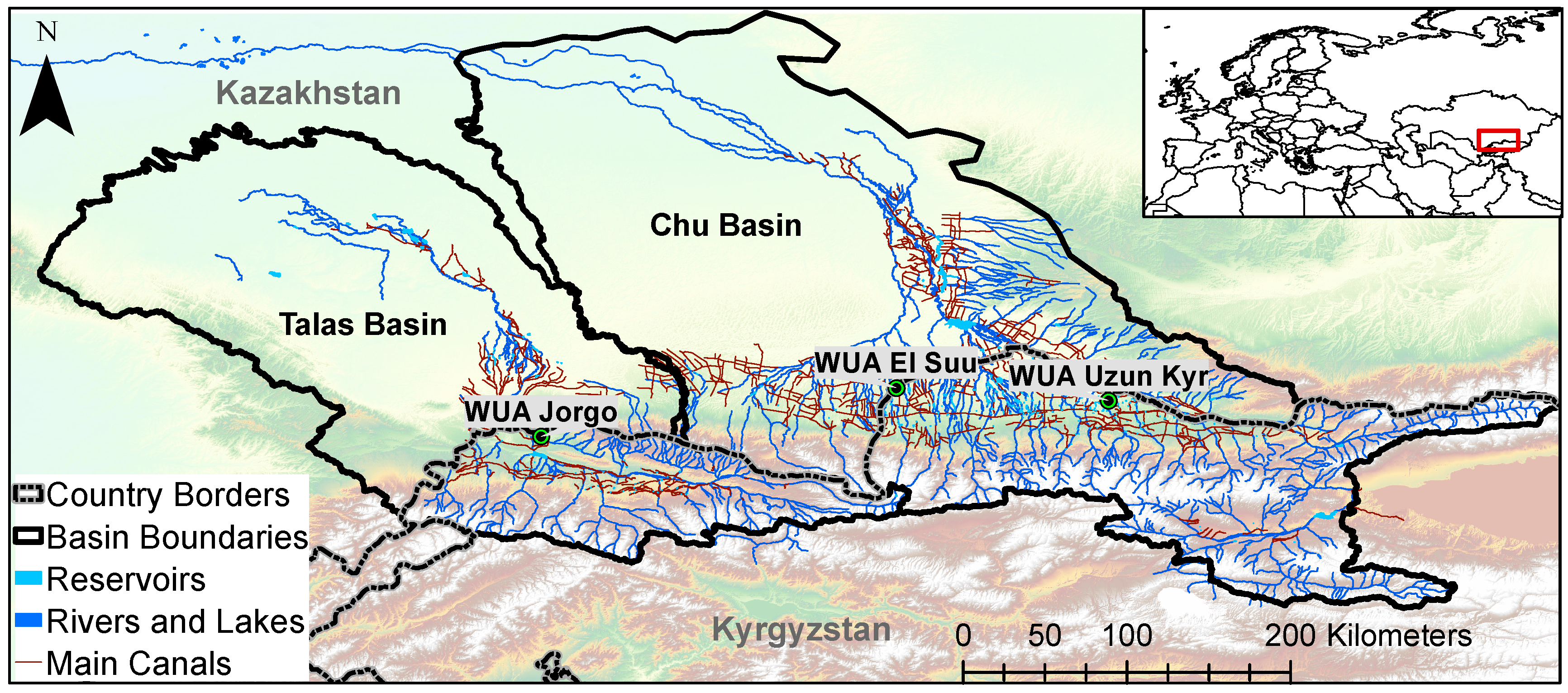
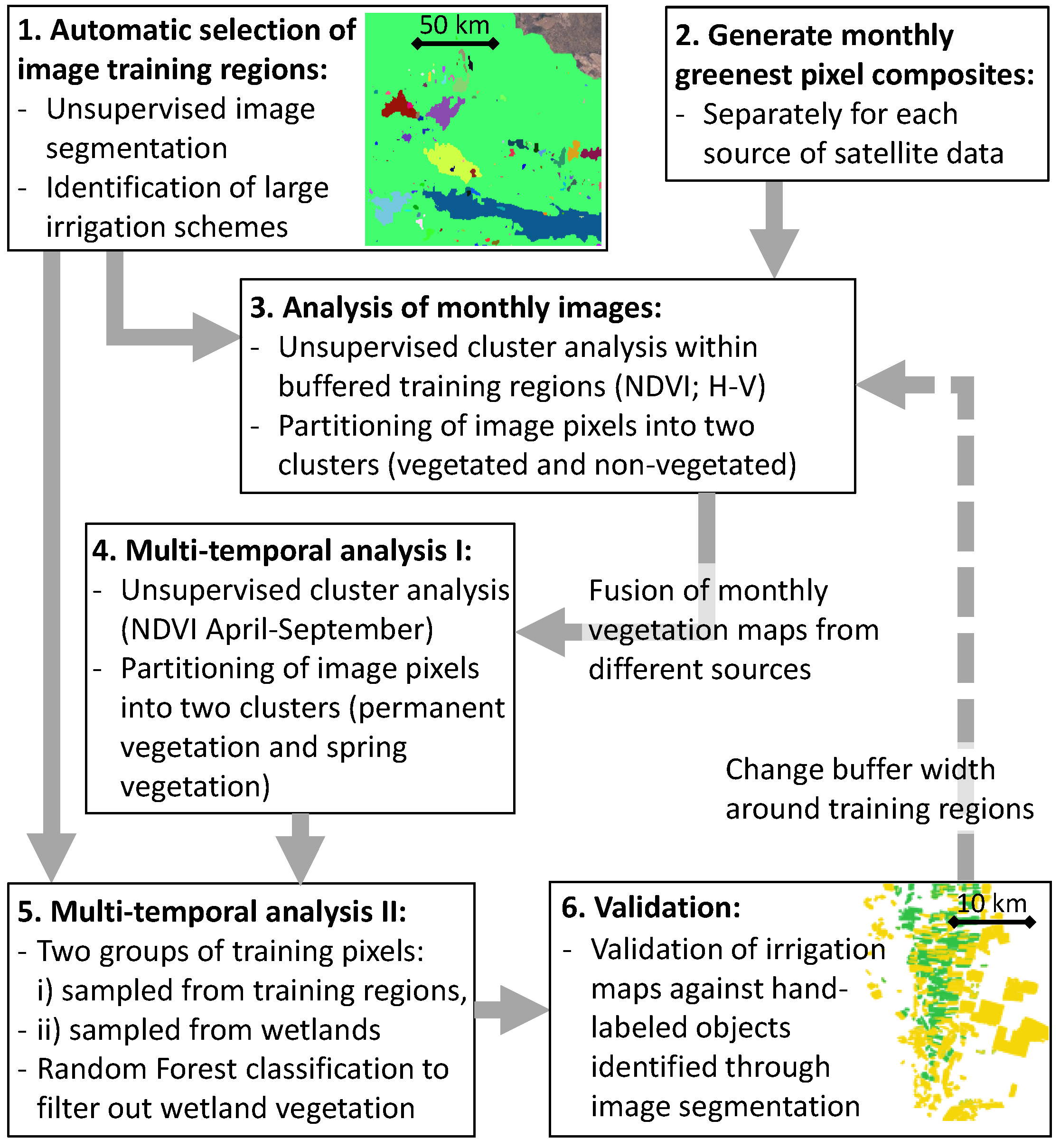
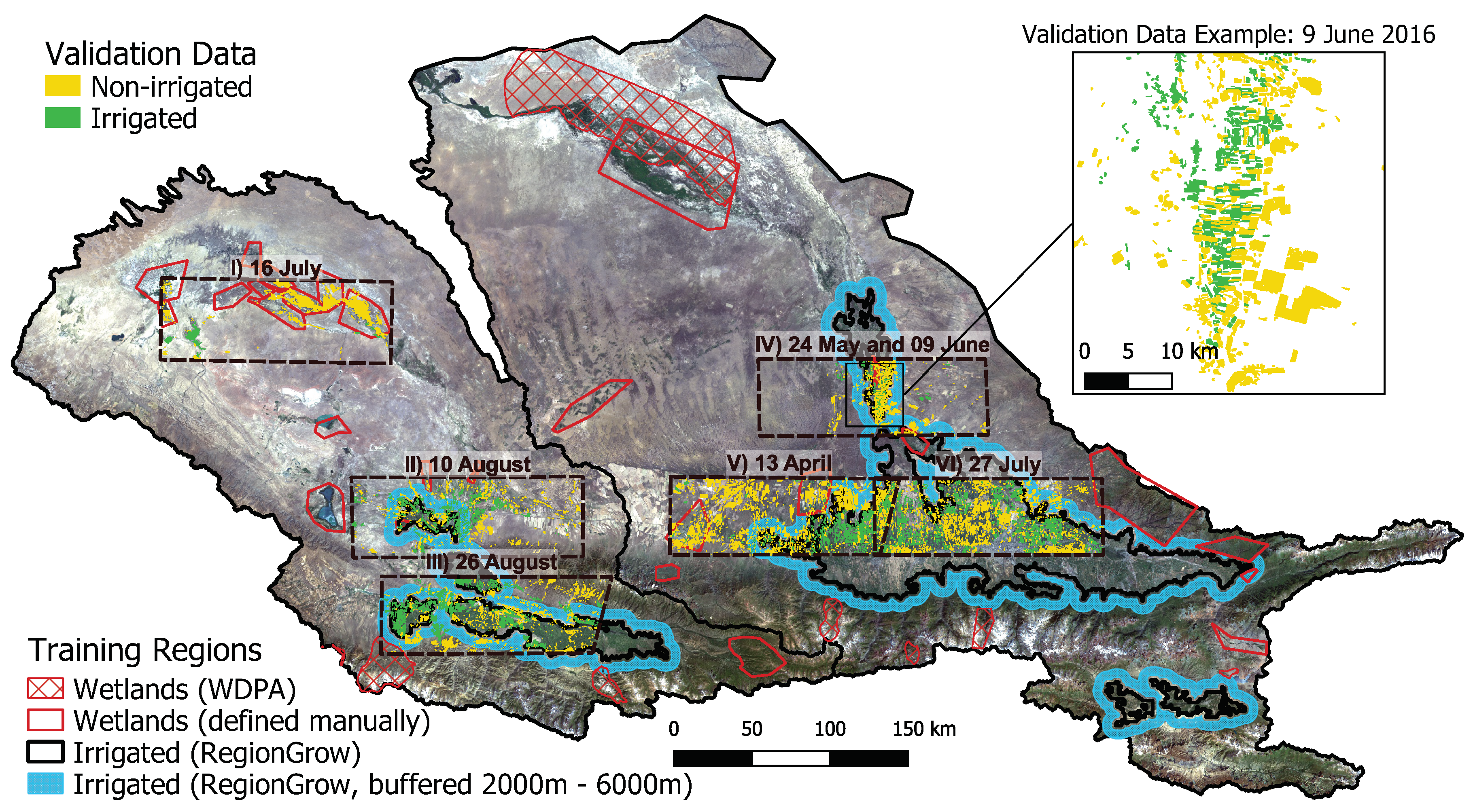
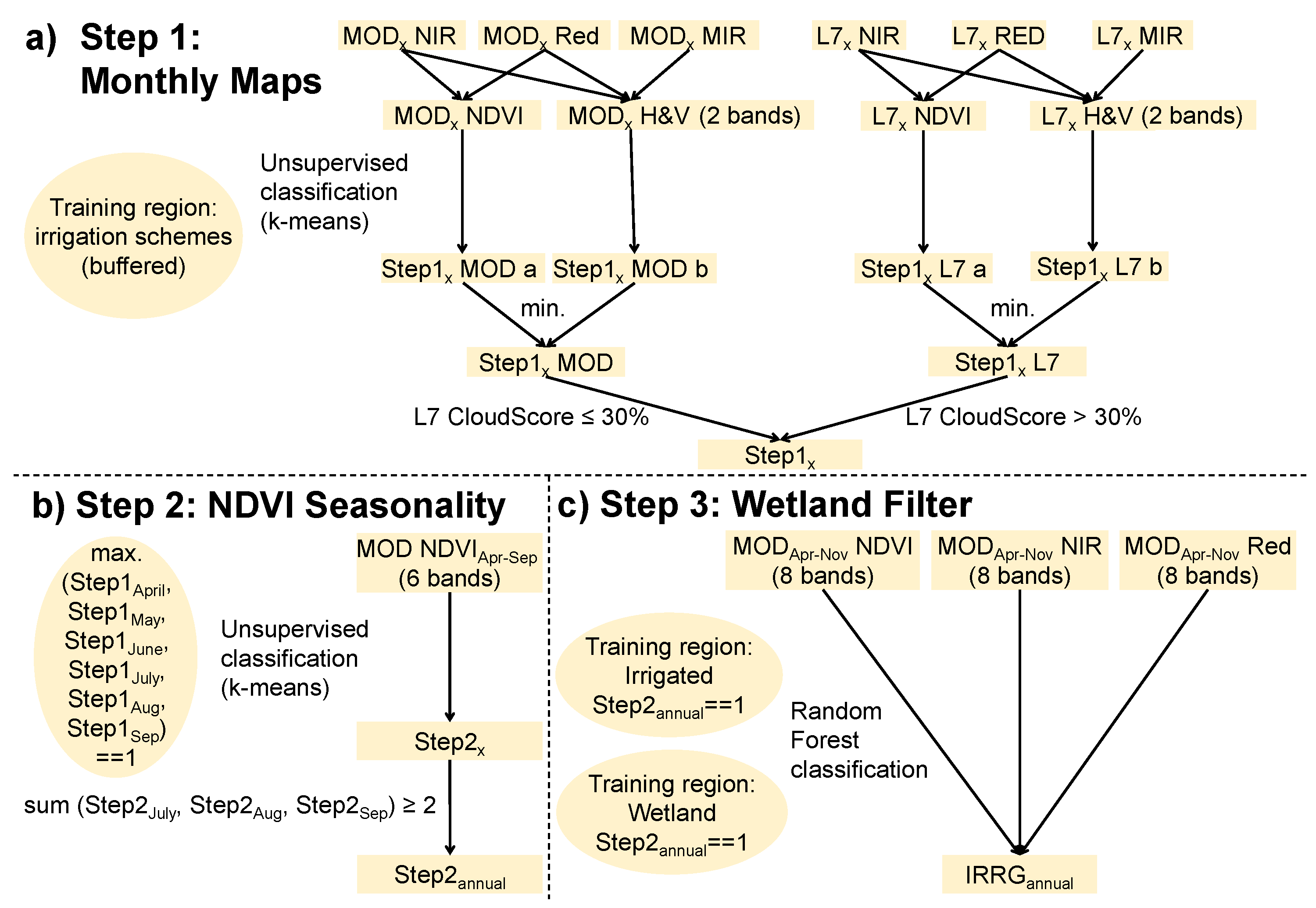
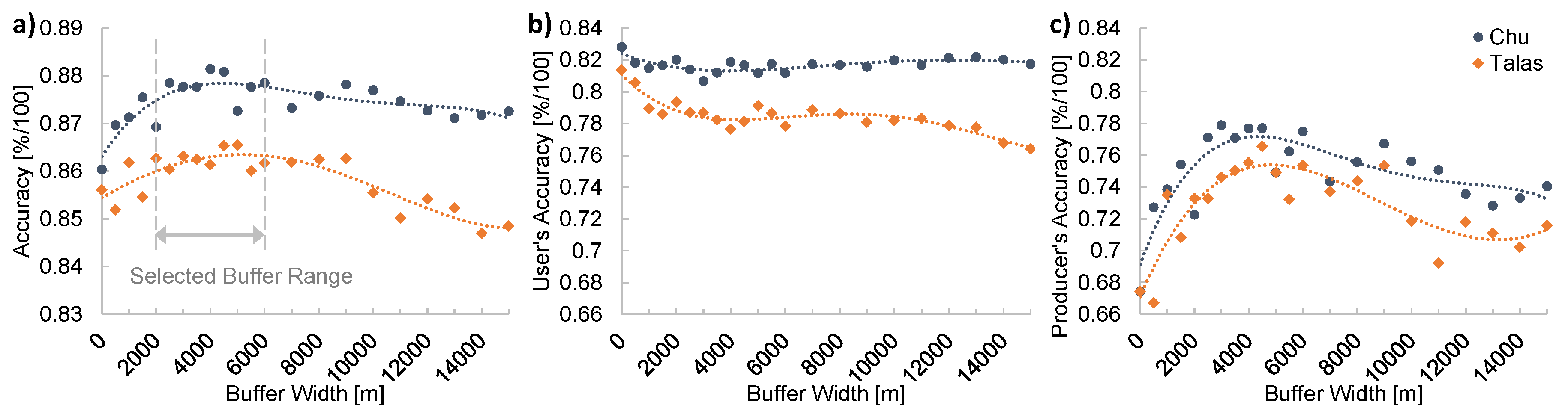
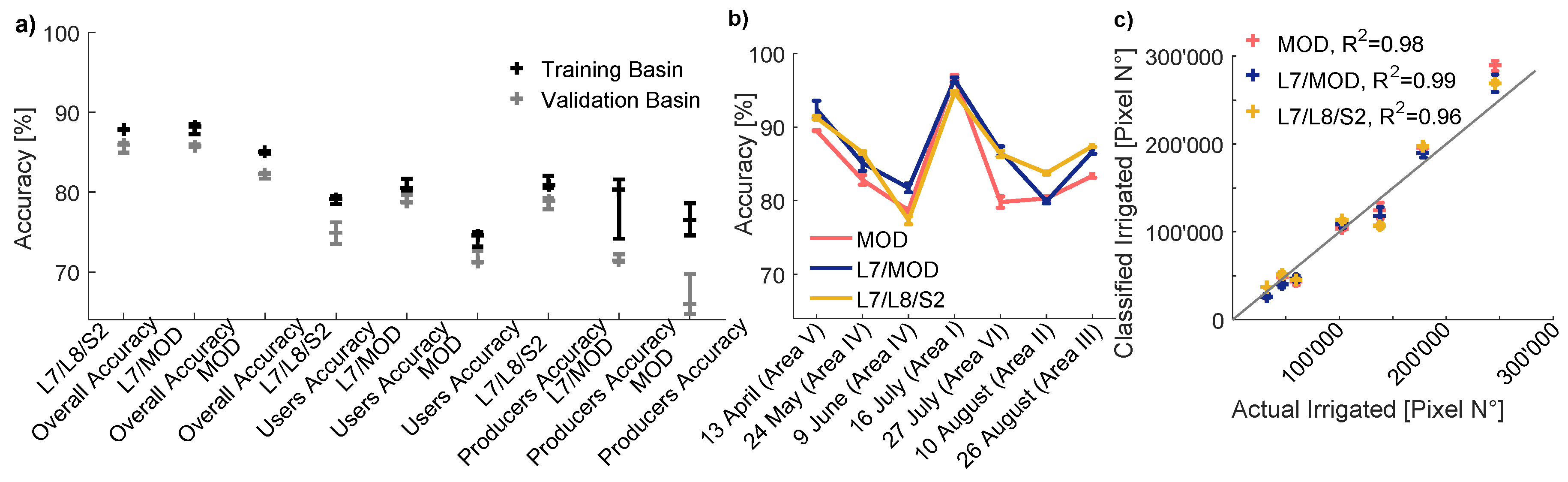
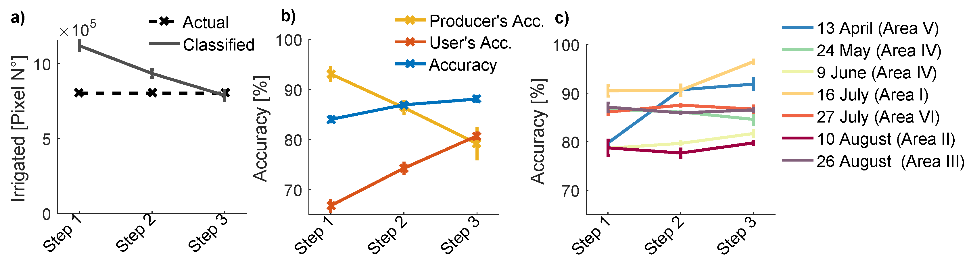
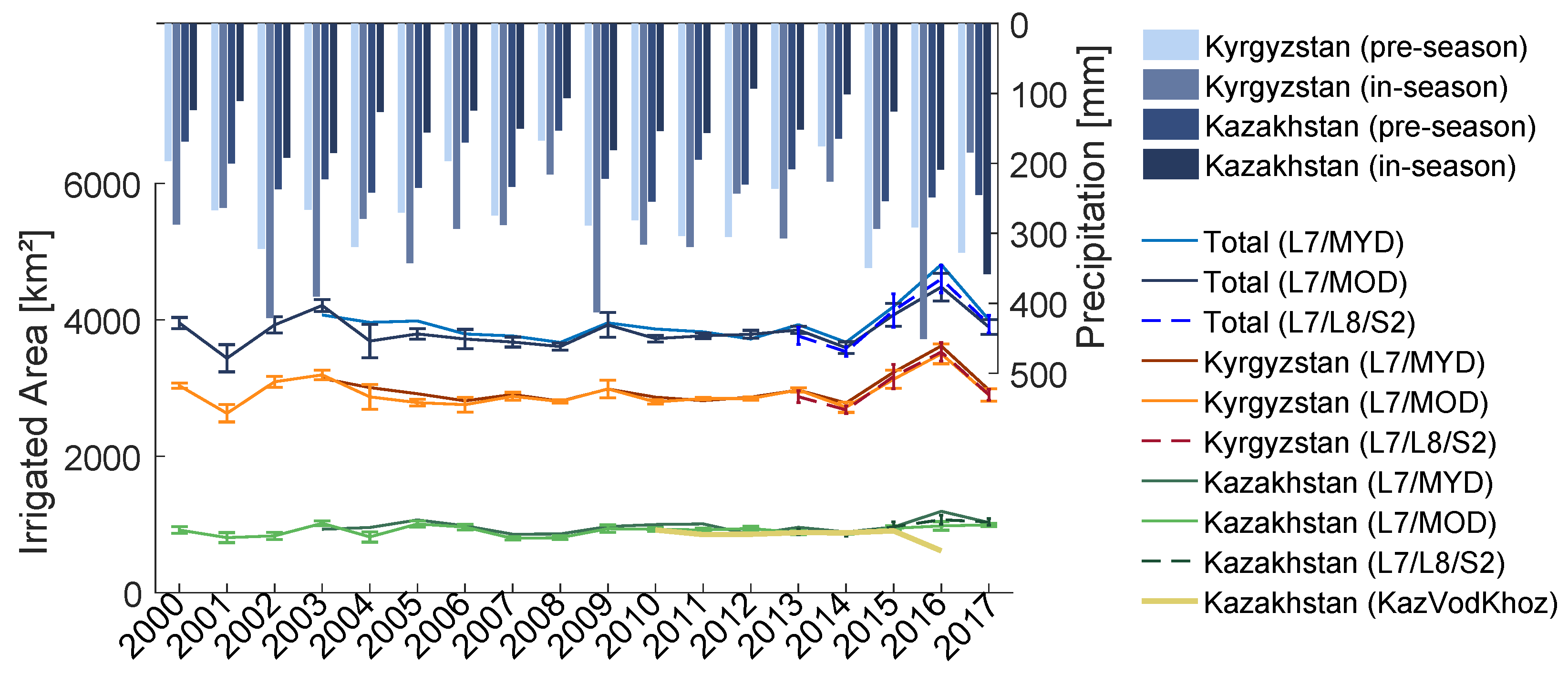
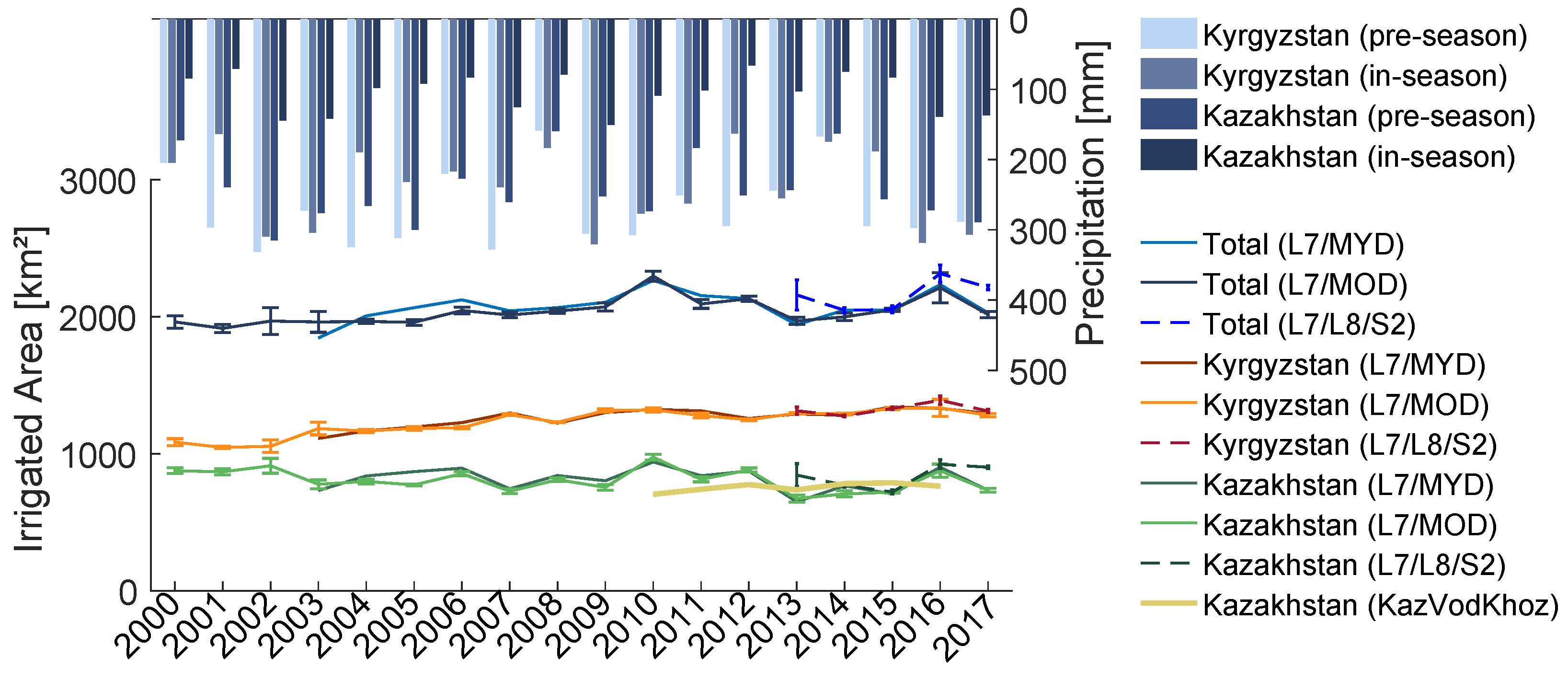
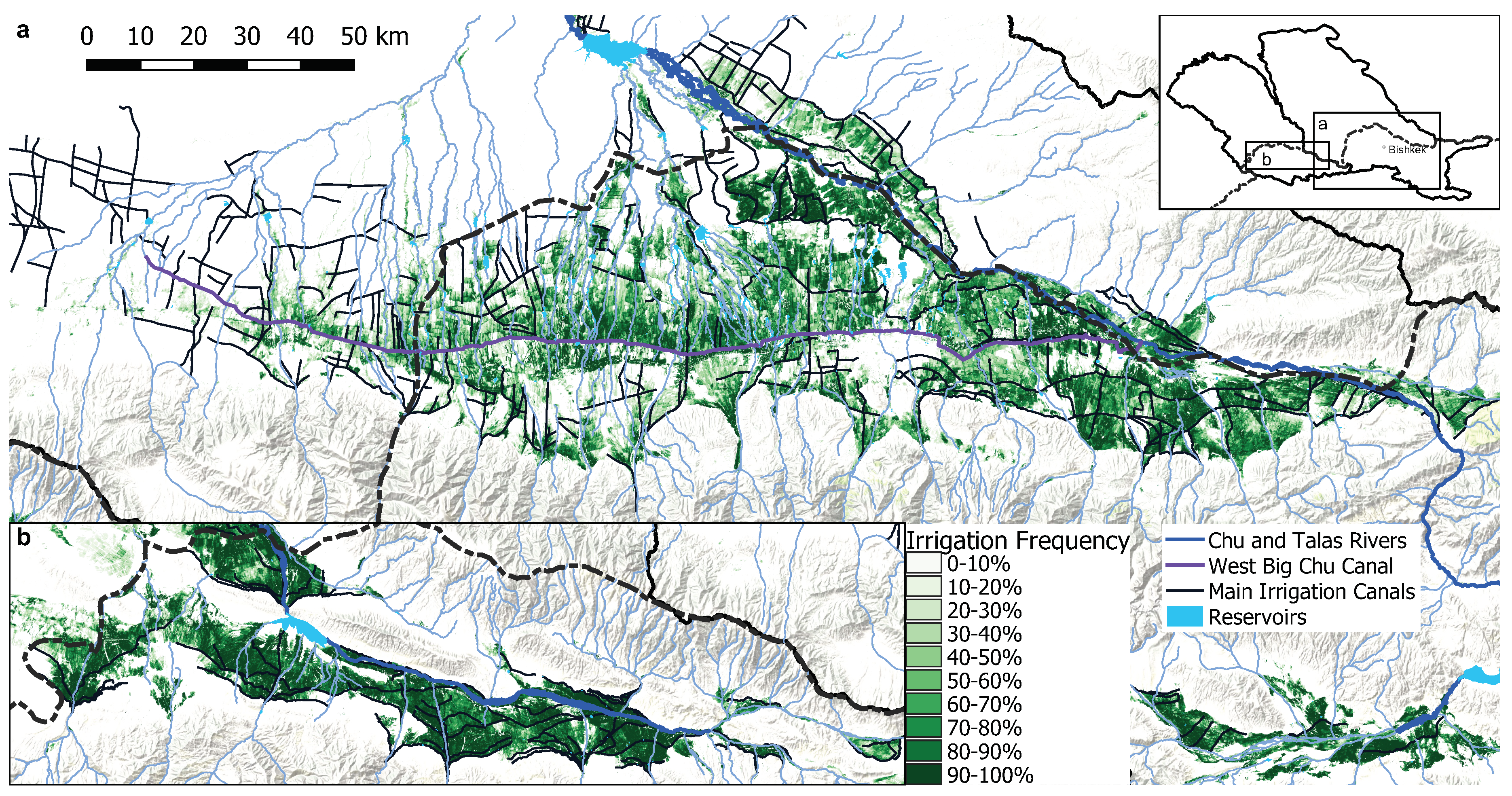
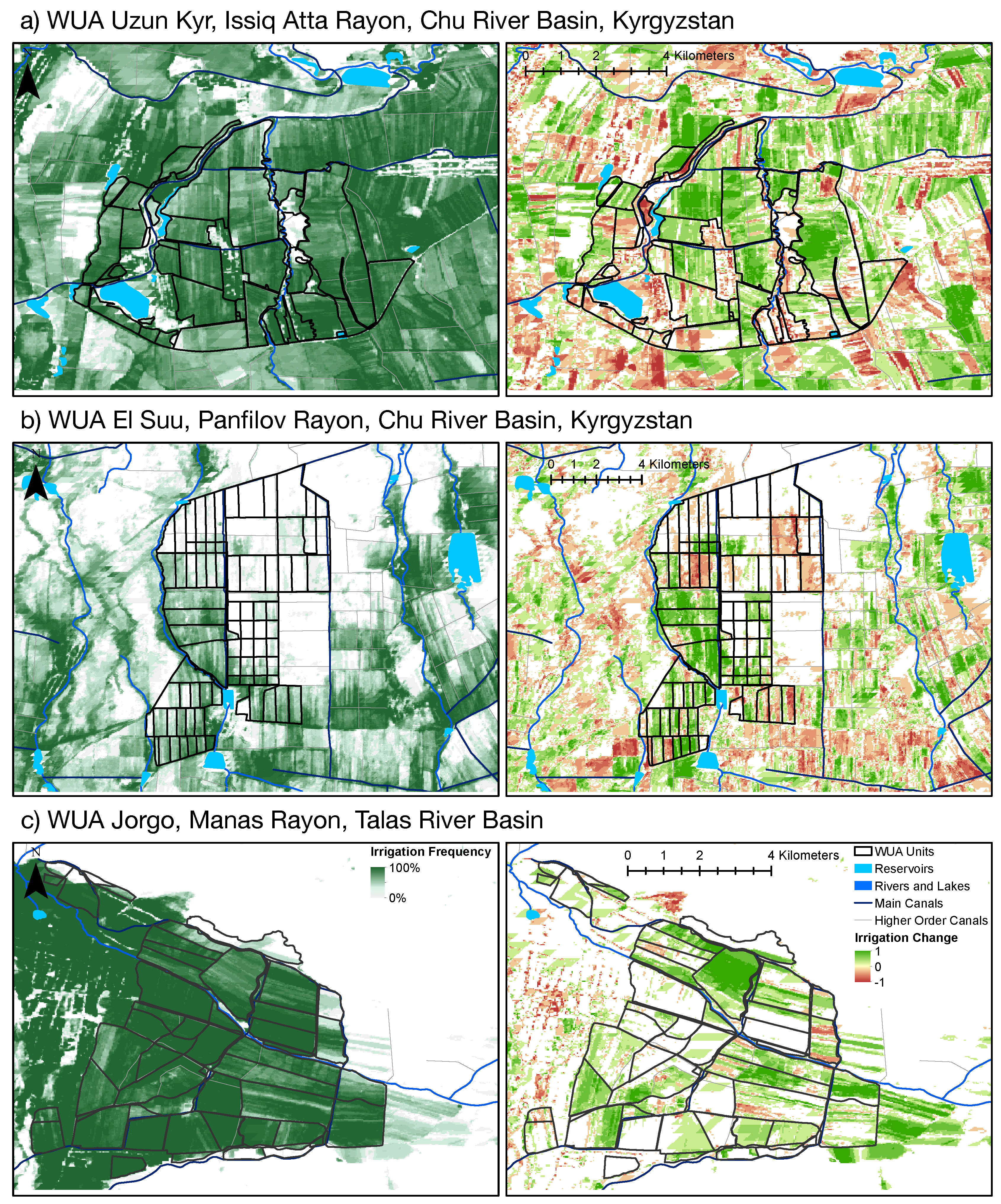
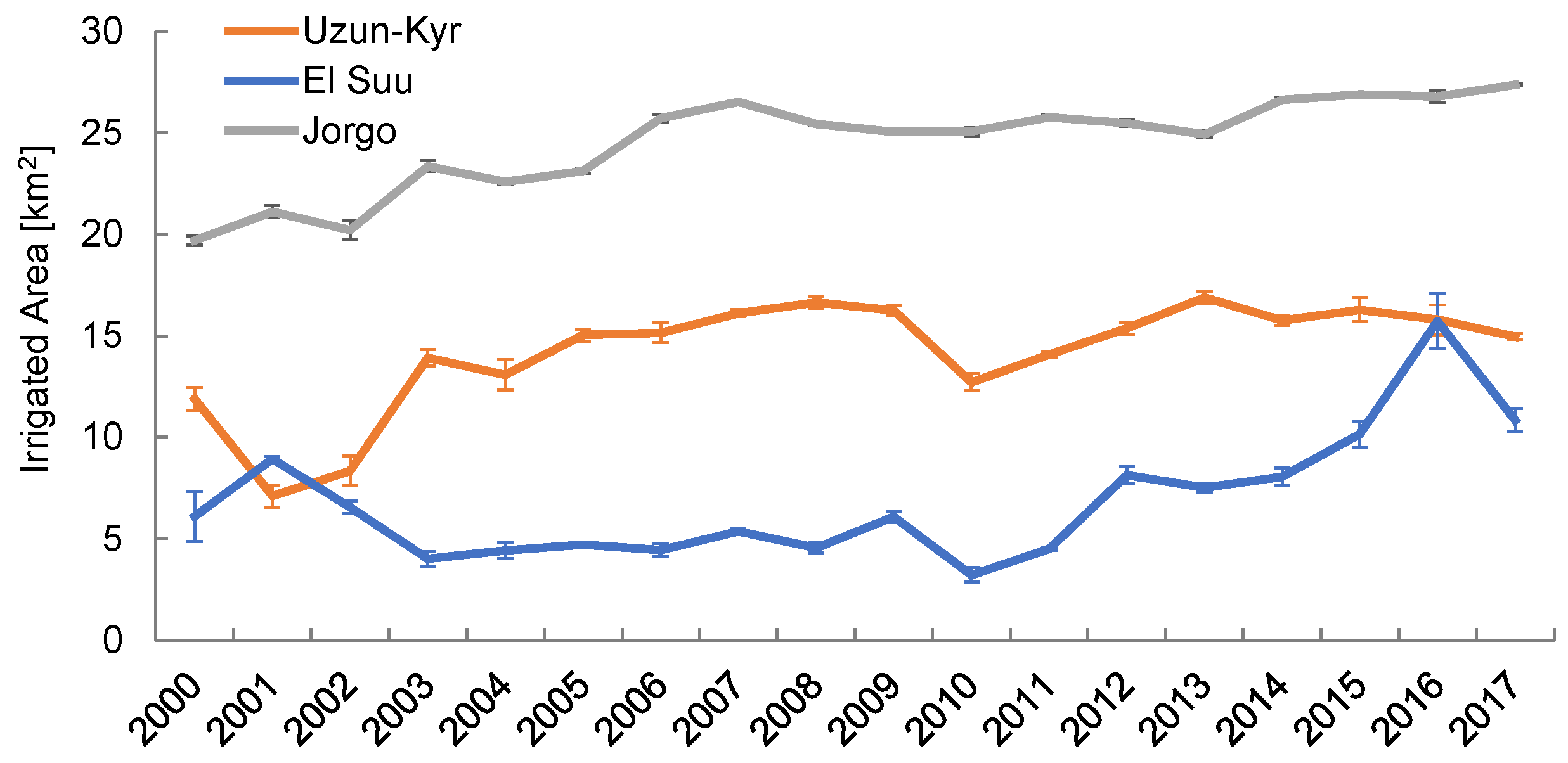
Table 1.
Remote-sensing data used.
| Satellite | Code | GEE ImageCollection ID | Available Since | Used Bands | Spatial/Temporal Resolution |
|---|---|---|---|---|---|
| Landsat 7 | L7 | LANDSAT/LE07/C01/T1_TOA | 1999 | B1, B2, B3 | 30 m/16 days |
| Landsat 8 | L8 | LANDSAT/LC08/C01/T1_TOA | 2013 | B2, B3, B4 | 30 m/16 days |
| Sentinel 2 | S2 | COPERNICUS/S2 | 2015 | B4, B8A, B12 | 10–20 m/10 days |
| MODIS Terra | MOD | MOD09Q1 | 2000 | B1, B2 | 250 m/Daily |
| MODIS Terra | MOD | MOD09A1 | 2000 | B7 | 500 m/Daily |
| MODIS Aqua | MYD | MYD09Q1 | 2003 | B1, B2 | 250 m/Daily |
| MODIS Aqua | MYD | MYD09A1 | 2003 | B7 | 500 m/Daily |
Table 2.
Summary error and uncertainty statistics of annual irrigated areas derived from the L7/MOD product. ‘Buffer’ represents the mean uncertainty that is due to the uncertainty in optimal buffer widths around image training regions. The values in columns ‘L7/MYD’ and ‘L7/L8/S2’ represent the RMSE of the two products with respect to L7/MOD. ‘KazVodKhoz’ are data provided by the Zhambyl branch of the Republican State Enterprise with the same name and the values here represent the RMSE with respect to L7/MOD annual irrigated areas.
| Buffer 2000–2017 | L7/MYD 2003–2017 | L7/L8/S2 2013–2017 | KazVodKhoz 2010–2016 | |
|---|---|---|---|---|
| Talas (KYG) | 1.4% | 1.8% | 2.3% | - |
| Talas (KAZ) | 2.7% | 4.5% | 15.2% | 16.0% |
| Talas | 1.8% | 2.6% | 4.2% | - |
| Chu (KYG) | 2.7% | 1.5% | 1.7% | - |
| Chu (KAZ) | 4.5% | 8.2% | 5.0% | 16.9% * |
| Chu | 2.9% | 3.7% | 2.0% | - |
* KazVodKhoz 2010–2015: 5.1%.
Table 3.
Summary statistics of the classified irrigated areas at river basin and riparian countries scales according to the L7/MOD product. b is the estimated Sen’s Slope, CI its confidence interval, A is the change in irrigated area with respect to the year 2000 according to the Sen’s Slope estimate and Cor P is the correlation coefficient between annual irrigated areas and pre- and in-season precipitation, respectively. Statistically significant trends or correlations are indicated.
| Irr. Area | mean (km2) | min (km2) | max (km2) | bsen (km2/year) | 95% CI (km2/year) | ΔA2000–2017 | Cor P (pre-seas.) | Cor P (in-seas.) |
|---|---|---|---|---|---|---|---|---|
| Talas | 2038 | 1916 | 2297 | 11.0 ** | [3.1 18.8] | 9.5% | 0.07 | 0.18 |
| Talas (KYG) | 1230 | 1047 | 1335 | 14.5 *** | [9.8 19.6] | 22.8% | −0.04 | 0.24 |
| Talas (KAZ) | 808 | 673 | 976 | −6.4 | [−13.5 2.1] | −12.3% | 0.13 | −0.02 |
| Chu | 3840 | 3437 | 4481 | 11.5 | [−13.9 32.9] | 4.9% | 0.39 | 0.71 *** |
| Chu (KYG) | 2931 | 2630 | 3502 | 6.9 | [−14.9 24.6] | 3.9% | 0.33 | 0.67 ** |
| Chu (KAZ) | 909 | 796 | 1018 | 4.4 | [−3.5 11.7] | 8.2% | 0.24 | 0.47 * |
*** Significant at the 0.001 level; ** Significant at the 0.01 level; * Significant at the 0.1 level.
© 2018 by the authors. Licensee MDPI, Basel, Switzerland. This article is an open access article distributed under the terms and conditions of the Creative Commons Attribution (CC BY) license (http://creativecommons.org/licenses/by/4.0/).
Share and Cite
MDPI and ACS Style
Ragettli, S.; Herberz, T.; Siegfried, T. An Unsupervised Classification Algorithm for Multi-Temporal Irrigated Area Mapping in Central Asia. Remote Sens. 2018, 10, 1823. https://doi.org/10.3390/rs10111823
AMA Style
Ragettli S, Herberz T, Siegfried T. An Unsupervised Classification Algorithm for Multi-Temporal Irrigated Area Mapping in Central Asia. Remote Sensing. 2018; 10(11):1823. https://doi.org/10.3390/rs10111823
Chicago/Turabian StyleRagettli, Silvan, Timo Herberz, and Tobias Siegfried. 2018. "An Unsupervised Classification Algorithm for Multi-Temporal Irrigated Area Mapping in Central Asia" Remote Sensing 10, no. 11: 1823. https://doi.org/10.3390/rs10111823
Note that from the first issue of 2016, this journal uses article numbers instead of page numbers. See further details here.