Article

Underestimates of Grassland Gross Primary Production in MODIS Standard Products

1
Key Laboratory of Land Surface Pattern and Simulation, Institute of Geographic Sciences and Natural Resources Research, Chinese Academy of Sciences, Beijing 100101, China
2
College of Geography and Environment, Shandong Normal University, Jinan 250358, China
3
University of Chinese Academy of Sciences, Beijing 100049, China
4
Department of Microbiology and Plant Biology, and Center for Spatial Analysis, University of Oklahoma, Norman, OK 73019, USA
5
Institute of Remote Sensing and Digital Earth, Chinese Academy of Sciences, Beijing 100094, China
6
Ministry of Education Key Laboratory of Biodiversity Science and Ecological Engineering, Institute of Biodiversity Science, Fudan University, Shanghai, 200438, China
*
Authors to whom correspondence should be addressed.
Remote Sens. 2018, 10(11), 1771; https://doi.org/10.3390/rs10111771
Submission received: 26 September 2018 / Revised: 1 November 2018 / Accepted: 5 November 2018 / Published: 8 November 2018
(This article belongs to the Special Issue Terrestrial Carbon Cycle)

Abstract

:
As the biggest carbon flux of terrestrial ecosystems from photosynthesis, gross primary productivity (GPP) is an important indicator in understanding the carbon cycle and biogeochemical process of terrestrial ecosystems. Despite advances in remote sensing-based GPP modeling, spatial and temporal variations of GPP are still uncertain especially under extreme climate conditions such as droughts. As the only official products of global spatially explicit GPP, MOD17A2H (GPPMOD) has been widely used to assess the variations of carbon uptake of terrestrial ecosystems. However, systematic assessment of its performance has rarely been conducted especially for the grassland ecosystems where inter-annual variability is high. Based on a collection of GPP datasets (GPPEC) from a global network of eddy covariance towers (FluxNet), we compared GPPMOD and GPPEC at all FluxNet grassland sites with more than five years of observations. We evaluated the performance and robustness of GPPMOD in different grassland biomes (tropical, temperate, and alpine) by using a bootstrapping method for calculating 95% confident intervals (CI) for the linear regression slope, coefficients of determination (R2), and root mean square errors (RMSE). We found that GPPMOD generally underestimated GPP by about 34% across all biomes despite a significant relationship (R2 = 0.66 (CI, 0.63–0.69), RMSE = 2.46 (2.33–2.58) g Cm−2 day−1) for the three grassland biomes. GPPMOD had varied performances with R2 values of 0.72 (0.68–0.75) (temperate), 0.64 (0.59–0.68) (alpine), and 0.40 (0.27–0.52) (tropical). Thus, GPPMOD performed better in low GPP situations (e.g., temperate grassland type), which further indicated that GPPMOD underestimated GPP. The underestimation of GPP could be partly attributed to the biased maximum light use efficiency (εmax) values of different grassland biomes. The uncertainty of the fraction of absorbed photosynthetically active radiation (FPAR) and the water scalar based on the vapor pressure deficit (VPD) could have other reasons for the underestimation. Therefore, more accurate estimates of GPP for different grassland biomes should consider improvements in εmax, FPAR, and the VPD scalar. Our results suggest that the community should be cautious when using MODIS GPP products to examine spatial and temporal variations of carbon fluxes.

Graphical Abstract

1. Introduction

Gross primary productivity (GPP), which is also known as the rate of photosynthesis, is the biggest carbon flux of terrestrial ecosystems [1]. This carbon flux plays an important role in the terrestrial carbon cycle. GPP is also the basis for ecosystem services such as food, fuel, and wood products [2]. The ability to accurately track the spatial and temporal variability of GPP is fundamental for understanding the biogeochemical dynamics of terrestrial ecosystems [3,4]. Therefore, it is critical for us to accurately estimate GPP and further understand the trends and variations of global and regional carbon uptake. However, there still exist considerable uncertainties in GPP estimation, which has attracted plenty of attention [5,6,7].
Satellite remote sensing provides an unprecedented and practical opportunity to estimate ecosystem GPP at large scales by using a diagnostic approach. Numerous remote sensing models have been proposed including the Global Production Efficiency Model (GLOPEM) [8], the Carnegie-Ames-Stanford Approach model (CASA) [9], the Vegetation Photosynthesis Model (VPM) [10,11], the light use efficiency model (EC-LUE) [12], and the net photosynthesis model (PSN) [13]. The Moderate Resolution Imaging Spectroradiometer (MODIS) primary production products (MOD17A2) based on the PSN model are open access datasets with high temporal and spatial resolutions that allow for the monitoring of global GPP at the 1-km resolution every eight days [14]. Previous studies using different light use efficiency (LUE) models estimated global GPP ranging from 105 to 177 P g C a−1 [15,16] with a considerable uncertainty. Yuan et al. [17] compared seven LUE models and they found that only two models (EC-LUE and CFlux) showed higher correlations between GPP derived from eddy covariance (GPPEC) and modeled GPP and performed better in simulating inter-annual variability of GPP than others. Furthermore, the performances of different models are not the same among all vegetation types or biomes [18,19]. As the only official global GPP products (MOD17A2/MOD17A2H), the MODIS GPP (GPPMOD) products have been widely used in addressing scientific questions on terrestrial carbon uptake and carbon cycle [20,21]. For example, MOD17A2 has been used to understand the drought impact on global carbon uptake of terrestrial ecosystems [22].
However, there is still a great discrepancy about the reliability of GPPMOD when compared with in-situ data collected in different locations [23]. Due to the unavailability of directly measured GPP data, the validation of MODIS GPP products is still challenging. The eddy covariance technique is an effective approach to evaluate GPP on the landscape scale. A previous study found that the GPPMOD was reliable and matched well with GPPEC in the forest biome at Vancouver Island, Canada [24]. However, there are many studies that have highlighted the uncertainties of GPPMOD data in different ecosystem types. For example, Turner et al. [25] pointed out that the GPPMOD underestimated GPP at hardwood forest sites and, yet, agreed well with GPPEC data at boreal forest sites. In terms of savanna ecosystems, Leuning et al. [26] found that the GPPMOD performed differently for tropical wet/dry savannas. It overestimated GPP during the dry season and arid summer but matched very well during the two wet seasons. Consistent with that in Leuning et al. [26], GPPMOD underestimated GPP at dry sites located in the Sahel region, according to a study at 12 African sites of savanna ecosystems [27] while the product agreed well with GPPEC at wet sites. It showed that generally GPPMOD tend to be underestimated in drier forest ecosystems or savanna ecosystems. However, these studies were mostly based on the previous versions of the MODIS GPP product (Collection 4 or Collection 5), but the latest version (Collection 6) significantly improved the value of the maximum light use efficiency (for example, from 0.68 g C m−2 d−1 MJ−1 to 0.86 g C m−2 d−1 MJ−1 for grass) and the product footprint sizes (from 1 km to 500 m) [28]. Whether performance has improved for collection 6 or not in these ecosystems has not been studied on a global scale.
Compared to the forest and savanna biomes, validation of the MODIS GPP in grassland has also been studied extensively. Zhang et al. [29] found that MODIS data underestimated the mean annual GPP by 30% to 50% in the alpine meadow sites in China. Zhu et al. [30] also found that grassland GPP (MOD17A2) was underestimated at the Haibei grassland site during the summer. In the US, Doughty et al. [31] also found that GPPMOD performed poorly at the improved pasture sites, the native pasture sites, and the winter wheat sites when compared with GPPEC. However, these analyses were based primarily on limited spatial and temporal coverage of in situ observations. Regional-scale and global-scale evaluations of GPPMOD for grassland ecosystems has not yet been conducted. With the increasing global distribution of eddy flux towers and the formation of networks (e.g., FLUXNET [32], AmeriFLux [33], EuropeanFLux [34], AsiaFLux [12]), a large scale validation of GPP products has become feasible [24,35]. Recently, the latest global flux dataset of FLUXNET2015 [36] was released and it provided a great opportunity for the validation of GPPMOD for grassland ecosystems.
In this study, we aimed to conduct a systematic validation of GPPMOD for grassland ecosystems by using the FLUXNET2015 dataset. The overarching goals of this study are to: (1) examine the performance of GPPMOD across a network of grassland flux sites, (2) assess the uncertainties of GPPMOD under different grassland biomes (temperate, tropical, and alpine), and (3) discuss the potential reasons that cause the underestimation of GPP in the MOD17A2H products.

2. Materials and Methods

2.1. GPPMOD Algorithm

The MOD17A2H GPP product (Collection 6) is a standard global product with a 500-m spatial resolution and eight-day temporal resolution [22]. It is based on the light use efficiency approach, which calculates GPP by using the amount of photosynthetically active radiation (PAR) absorbed by vegetation over a growing season [37]. The algorithm was developed below.
G P P M O D = ε × F P A R × P A R
where ε is the actual light use efficiency, PAR is the photosynthetically active radiation (MJ m−2) per unit time, and FPAR is the fraction of PAR absorbed by vegetation canopy.
ε = ε m a x × T M I N s c a l a r × V P D s c a l a r
where εmax (g C m−2 d−1 MJ−1) is the maximum light use efficiency, which is given in a Biome Parameter Look-up Table (BPLUT) for each land cover type in the PSN model. The TMINscalar and VPDscalar are environmental stress factors of temperature (daily minimum temperature, Tmin, °C) and water (maximum daily vapor pressure deficit, VPD, Pa) and are parameterized according to Equations (3) and (4).
T M I N s c a l a r = { 1 T M I N > T M I N m a x ( T M I N T M I N m i n ) / ( T M I N m a x T M I N m i n ) T M I N m i n T M I N T M I N m a x 0 T M I N < T M I N m i n
V P D s c a l a r = { 0 V P D > V P D m a x ( V P D m a x V P D ) / ( V P D m a x V P D m i n ) V P D m i n V P D V P D m a x 1 V P D < V P D m i n
where TMIN and VPD are the daily minimum temperature (°C) and the average vapor pressure deficit (Pa), TMINmax and VPDmax are the daily minimum temperature and the average vapor pressure deficit at which ε = εmax, and TMINmin and VPDmin are the daily minimum temperature and average vapor pressure deficit at which ε = 0 [28,38]. These parameters were determined, according to the BPLUT. The NASA Global Modeling and Assimilation Office (GMAO) provided input data for the GPPMOD algorithm including global meteorological simulations of incoming PAR, daily maximum/minimum temperature, and daily maximum/minimum VPD. We downloaded MODIS Collection 6 data for 2000 to 2014 and we extracted GPPMOD from pixels with the 500-m resolution in which the flux towers were located. GPPMOD for each site was transformed from monthly totals to monthly means and were converted from kg C m−2 to g C m−2.

2.2. CO2 Eddy Flux and Meteorological Data

We used the FLUXNET2015 datasets (http://www.fluxdata.org) to evaluate the performance of GPPMOD. The FLUXNET2015 datasets include carbon dioxide (CO2), water vapor, energy fluxes, shortwave and longwave radiations, photosynthetically active radiation, temperature, and precipitation for each flux tower site. We selected all grassland flux tower sites across the world with more than five years of observations between 2000 and 2014 using the 500-m resolution. The selection included 15 grassland sites with eddy covariance towers. All of these were included in this study (Figure 1 and Table 1). The meteorological data including precipitation, air temperature, solar radiation, and VPD were used in this study. We used the gap-filled GPP data derived from the Marginal Distribution Sampling (MDS) method for gap-filling and the night-time partitioning method for the net ecosystem exchange (NEE) partitioning [39]. The daily GPPEC values were transformed to monthly GPPEC values (g C m−2 day−1) for a comparison with the GPPMOD.

2.3. Evaluation of Model Performance

In this study, GPPMOD was evaluated against GPPEC. First, according to the climate characteristics of the grassland sites, we merged the 15 grassland sites into three grassland biomes, i.e., temperate, tropical, and alpine grasslands. Second, we evaluated the model performance by comparing the seasonal dynamics of GPPMOD and GPPEC by using the linear regression model (GPPEC = a × GPPMOD + b). During the evaluation, modeled data (GPPMOD) are plotted on the x-axis and observation data (GPPEC) on the y-axis. This avoids estimating spurious biases in the representation [40]. The coefficient of determination (R2) was used to evaluate the models’ explanatory abilities for variances in GPP. Third, the root mean squared errors (RMSE) were calculated to quantify the agreement between GPPEC and GPPMOD during the plant-growing season (GPP > 1 g C m−2 day−1).
R M S E = 1 n × n = 1 n ( X i Y i ) 2
where n is the total number of sample points and Xi and Yi represent the observed and simulated values, respectively.
We used the bootstrapping method to provide confidence intervals necessary to determine whether these indicators (slopes, RMSE, and R2) are different or not and repeated sampling for 4000 times in the bootstrapping analysis.

2.4. Estimation of ε m a x

The ε m a x is an important parameter in the GPPMOD algorithm. The ε m a x for vegetation types can be obtained from an analysis of gross ecosystem exchange of CO2 and photosynthetic photon flux density (PPFD) at an eddy flux tower site [41,42]. In this study, we used a nonlinear model between GPP and PPFD (at half-hour time step) data to estimate the ε m a x for each grassland site [43,44,45]. The abnormal observations (including zero values or extremely high values) have been excluded before fitting the function. The model is described below [42,43].
N E E = α × P P F D × G E E m a x α × P P F D G E E m a x R
where α is the apparent quantum yield and is assumed to be the ε m a x . R is the ecosystem respiration, GEEmax is the maximum gross ecosystem exchange (GEE), and NEE is the net ecosystem exchange.

3. Results

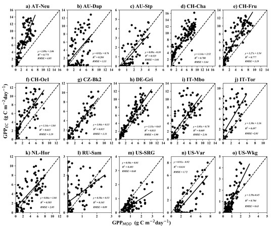
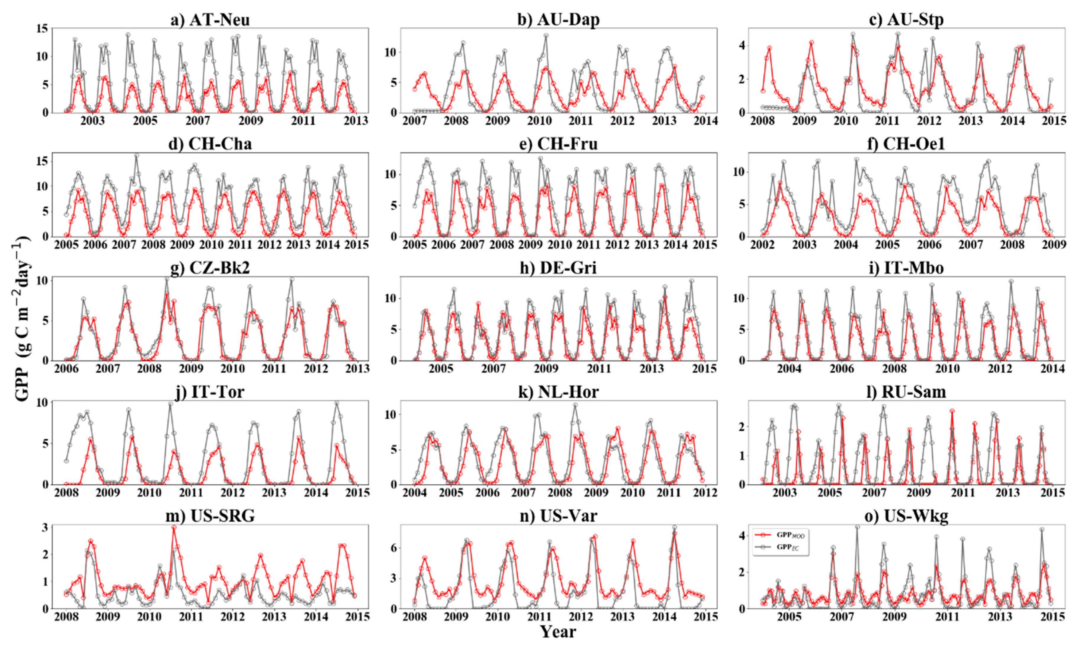
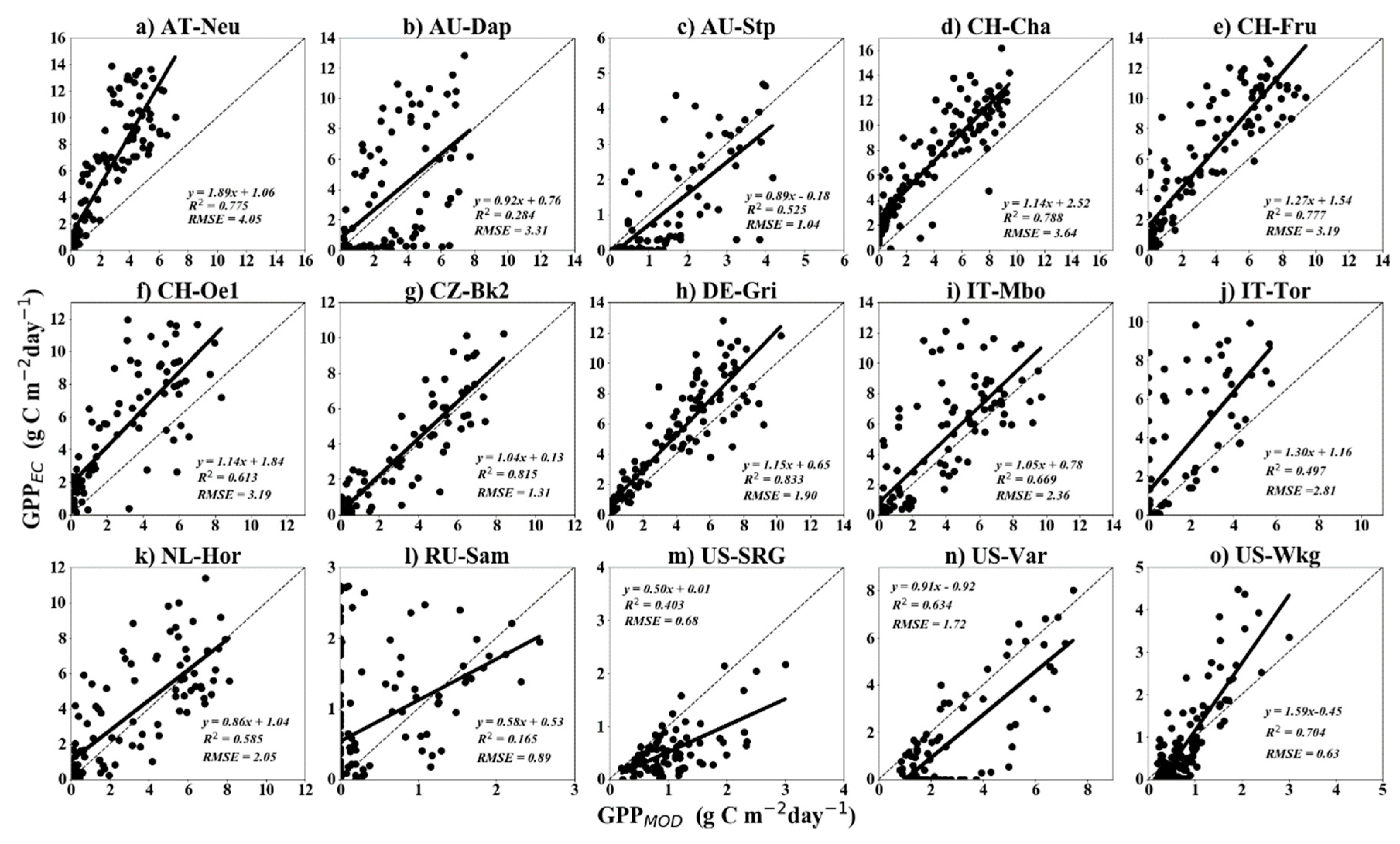
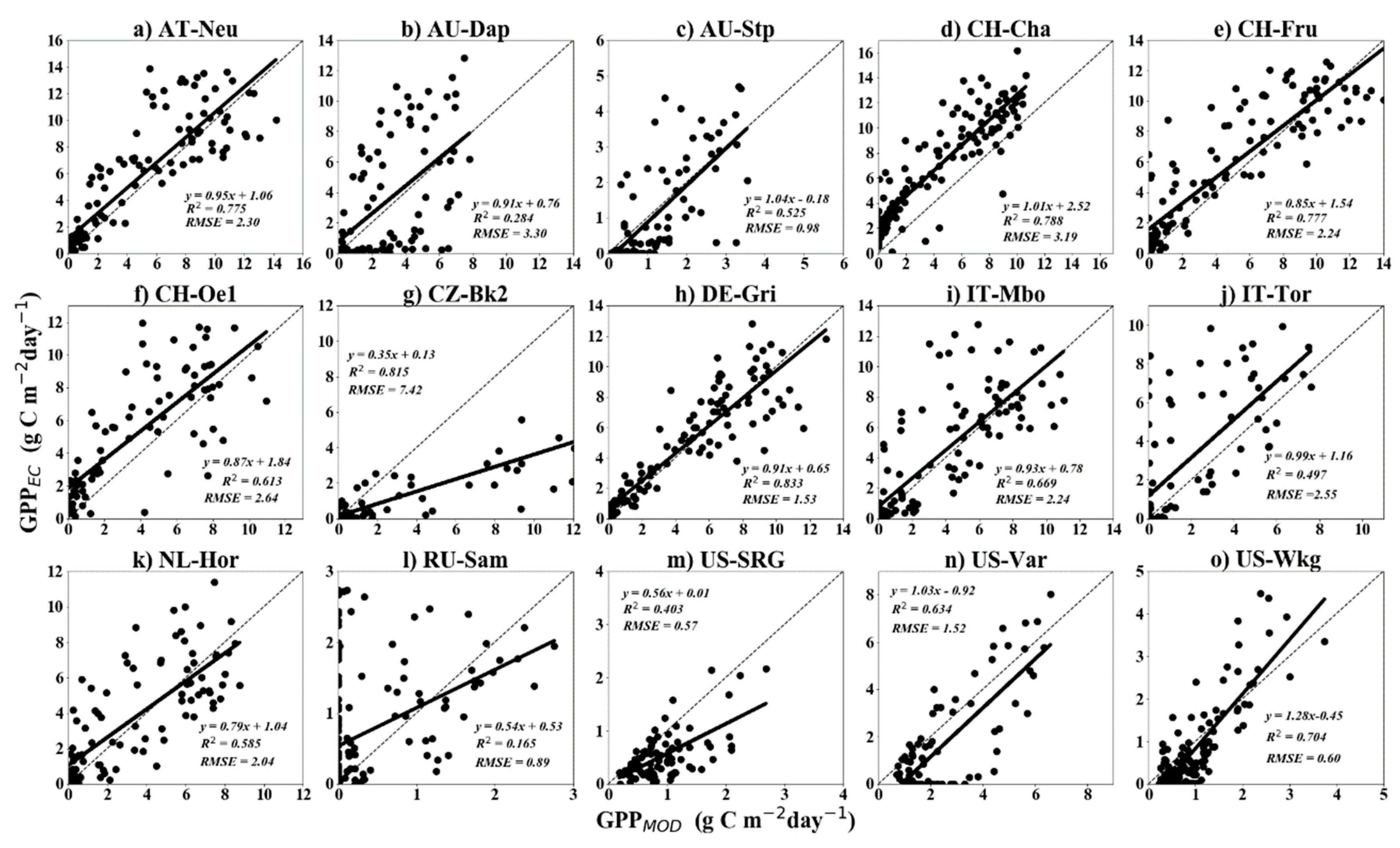
3.1. Comparison of GPPMOD and GPPEC

Figure 2 illustrates the seasonal variation of GPPMOD and GPPEC at all sites. GPPMOD and GPPEC exhibit consistency in the magnitudes and seasonal variations at most of the grassland sites. GPP values started near zero in the winter, began to increase in the spring, reached its peak during the summer, and decreased quickly after its peak (Figure 2). The GPPEC in most sites were underestimated by the GPPMOD. For example, the GPPEC were underestimated by 58.48%, 56.24%, and 53.25% in AT-Neu, RU-Sam, and IT-Tor, respectively (Figure 2a), ((l), and (j)). The coefficients of determination (R2) between GPPMOD and GPPEC varied from 0.17 (CI, 0.08–0.29) at the RU-Sam site to 0.83 (0.77–0.89) at the DE-Gri site with all being statistically significant at p < 0.05 (Figure 3) and all these analyses were tested with a 95% confidence interval (Table 2). The linear regression between GPPMOD and GPPEC showed that GPPMOD performed well at DE-Gri (R2 = 0.83 (0.77–0.89), RMSE = 1.90 (1.61–2.18) g Cm−2 day−1), CZ-Bk2 (R2 = 0.82 (0.74–0.88), RMSE = 1.31 (1.05–1.54) g Cm−2 day−1), CH-Cha (R2 = 0.79 (0.70–0.86), RMSE = 3.64 (3.29–4.00) g Cm−2 day−1), CH-Fru (R2 = 0.78 (0.71–0.84), RMSE = 3.19 (2.78–3.57) g Cm−2 day−1), and AT-Neu (R2 = 0.78 (0.72–0.83), RMSE = 4.05 (3.52–4.55) g Cm−2 day−1), but it performed poor at RU-Sam (R2 = 0.17 (0.08–0.29), RMSE = 0.89 (0.74–1.03) g Cm−2 day−1), AU-Dap (R2 = 0.28 (0.14–0.45), RMSE = 3.31 (2.88–3.70) g Cm−2 day−1), US-SRG (R2 = 0.40 (0.18–0.59), RMSE = 0.68 (0.58–0.77) g Cm−2 day−1), and IT-Tor (R2 = 0.50 (0.33–0.67), RMSE = 2.81 (2.23–3.34) g Cm−2 day−1) (Figure 3). Moreover, GPPMOD had a R2 of 0.66 (0.63–0.69) and RMSE of 2.46 (2.33–2.58) g Cm−2 day−1 for all grassland tower sites (Figure 4).

3.2. Model Performances in Different Grassland Biomes

We also considered the seasonal dynamic of GPPMOD by analyzing the relationship between GPPMOD and GPPEC within each grassland biome. The 15 flux sites were divided into three grassland biomes including the temperate, tropical, and alpine biomes. All analyses were tested with a 95% confidence interval (Table 3). Figure 5 shows the different relationships between GPPEC and GPPMOD for each biome type. From Figure 5, we find GPPMOD had better performance in a temperate grassland (R2 = 0.72 (0.68–0.75), RMSE = 2.40 (2.25–2.54) g Cm−2 day−1) than an alpine grassland (R2 = 0.64 (0.59–0.68), RMSE = 2.55 (2.30–2.79) g Cm−2 day−1) or a tropical grassland (R2 = 0.40 (0.27–0.52), RMSE = 2.45 (2.13–2.76) g Cm−2 day−1) (Figure 5). Furthermore, MODIS GPP products underestimated GPP about 4% for the tropical grassland, 29% for the temperate grassland, and 41% for the alpine grassland, respectively.

4. Discussion

4.1. Underestimation of MODIS GPP in Grasslands and Comparison with Previous Studies

This study showed that GPPMOD had a promising ability to explain GPPEC variance (R2 = 0.66 (0.63–0.69) and RMSE = 2.46 (2.33–2.58) g Cm−2 day−1) at grassland sites, but GPPMOD consistently underestimated GPPEC (Figure 4). We also found that different grassland biomes had different performances. Specifically, GPPMOD performed better in the temperate grassland sites than in the alpine and tropical grassland sites (Figure 5).
This study indicated that GPPMOD substantially underestimated GPP in grasslands, which agreed with previous studies [29,30,31]. For instance, Zhang [29] used GPPEC measurements to verify GPPMOD over an alpine meadow on the Tibetan Plateau, which further pointed out that MOD17 GPP products underestimated the mean annual GPP by 30% to 50%. Turner et al. [46] also reported that GPPMOD underestimated GPP at desert grassland sites. Xiao [47] evaluated GPPMOD by using GPP data from eddy covariance flux towers and their results showed that the GPPMOD products underestimated GPP by 45% at the Walnut Gulch Kendall grassland site. Despite the wide use of GPPMOD to analyze inter-annual variation at regional scales in previous studies [48,49], the results from this study and the previously mentioned studies implied additional caution should be given when using GPPMOD for inter-annual and intra-annual variation analyses of GPP in grasslands. We found that GPPMOD underestimates observed GPP and that GPPMOD explained 66% (63%–69%) of the variance in GPPEC (R2 = 0.66 (0.63–0.69), RMSE = 2.46 (2.33–2.58) g Cm−2 day−1).
In addition, we found that the GPPMOD could explain more GPP variance for the temperate and alpine grassland sites than for the tropical grassland sites (Figure 5). Thus, GPPMOD performed better in lower GPP situations (e.g., drought condition and temperate grassland biome), which further illustrated that the GPPMOD tended to underestimate GPP.

4.2. Attributing Underestimation in Grassland GPP and Its Implications

In this study, GPPMOD explained GPPEC by 72% (68%–75%) at temperate grassland sites, 64% (59%–68%) at alpine grassland sites, and 40% (27%–52%) at tropical grassland sites (Figure 5). Potential reasons for the uncertainty in MODIS GPP products could be due to different factors such as maximum LUE, meteorological data, FPAR, and land cover/vegetation types [50].
These varied performances may be related to the maximum light use efficiency (εmax) [51]. For the MODIS GPP algorithm, εmax was determined by using the Biome Properties Look-Up (BPLUT) for given biome types, which was for 0.86 g C MJ−1 grass [38]. The underestimated εmax values could be the major reason for underestimates of GPP in the grasslands [51]. Based on the nonlinear model (Equation (6)), we estimated the εmax for each grassland site in this study (Table 4). In most sites (except for AU-Stp, US-SRG, and US-Var), the estimated values of εmax were larger than that used in the MOD17 GPP algorithm, which can partly explain the underestimation of the MODIS GPP in these grassland sites. Moreover, when the εmax used in the MOD17 GPP algorithm ( ε m a x -BPLUT) were simply replaced with the estimated εmax ( ε m a x -EST), the RMSEs were smaller than before (except for the site of CZ-Bk2) (Figure 6). This demonstrated that the εmax have an important influence on the result of the GPP estimation based on the MOD17 GPP algorithm. Previous studies have also suggested different εmax for different grassland biomes. For example, 1.31 g C MJ−1 for alpine grassland and 1.21 g C MJ−1 for tropical grassland [52,53]. Sjöström et al. [27] increased εmax for grasslands from 0.86 g C MJ−1 to 2.01 g C MJ−1, which improved the ability for GPPMOD to explain the variance of GPPEC from 25% to 74%.
There are also potential uncertainties from FPAR, which could affect the accuracy of GPPMOD. The GPPMOD algorithm directly used the MODIS FPAR products (MOD15A2H), which was derived from a radiative transfer model. The MODIS FPAR usually overestimated the “green” FPAR with a positive offset for barren land and was saturated at high GPP values. This behavior further affected ε and GPP estimation [54]. In this study, GPPMOD underestimated GPPEC for grassland ecosystems, which may be caused by the uncertainty of FPAR and the methods used to simulate FPAR. For example, Liu et al. [55] used a three-dimensional formulation of the radiative transfer process in the canopy and assessed FPARcanopy performances of scaled EVI (FPARchl1), NDVI, scaled NDVI (FPARchl2), and EVI. The results showed that the FPARcanopy of scaled EVI (FPARchl) improved the accuracy of GPPMOD for grasslands.
Another previous study [55] compared MODIS-FPAR and GLASS-FPAR (derived from the product of the Global Land Surface Satellite (GLASS)). MODIS-FPAR performed well with a higher R2 and a lower bias for mixed forests and cropland. However, GLASS-FPAR performed better in grasslands with a higher R2 and a lower bias [55]. Furthermore, Kucharik et al. [33] and Wu et al. [51] pointed out that the adaptive Savitzky-Golay filtered FPAR data could have better performance compared with the FPAR data based on the linear interpolation approach used in the MODIS algorithm. The adaptive SG method could maintain some intrinsic seasonal variability and keep reliable values of FPAR. Further uncertainties also arise due to the canopy photosynthesis saturation effects on the FPAR [56]. In this study, GPPMOD products underestimated GPP in tropical grassland sites because of the saturation of canopy photosynthesis. A previous study showed that the MODIS light use efficiency approach does not account for saturation of canopy photosynthesis under clear sky conditions in a tropical forest site [50]. Saturation can result in the underestimation of GPP with low values of FPAR but overestimation with high FPAR values [50]. The tropical grassland received solar radiation for extended periods and it was easy for canopy photosynthesis saturation to occur [57] especially in periods of drought. Previous studies also reported that saturation of canopy photosynthesis might occur on clear-sky days at the hourly and daily timescales [25,58,59].
The species composition of grassland ecosystems could also cause uncertainty in GPP estimates. Grasslands are dynamic ecosystems that often have diverse mixtures of C3 and C4 species, which have different light use efficiencies. Furthermore, the ratio of C3 and C4 species within a grassland can have high intra-annual and inter-annual variability [31]. Such community composition data is not available for all the FLUXNET sites. The effects of the composition of C3 and C4 grasses on GPP simulation is an interesting question, but it is beyond the scope of this specific study. However, a recent GPP product considering the C3 and C4 photosynthesis pathways showed improved performances in grassland ecosystems [60]. The water stress scalar could also have uncertainty when using VPD as a proxy of water stress in the PSN model. To decrease uncertainties, we suggest using long-term meteorological observation data or remote sensing-based water stress indicators [61] to quantify the water stress scalar especially in drought conditions. Furthermore, fundamental improvements could be made to GPPMOD products. For instance, the Soil Moisture Active Passive (SMAP) mission has two to three day temporal fidelity and an enhanced (≤9 km) spatial resolution that provide accurate global mapping of the freeze–thaw state and the surface soil moisture [62].

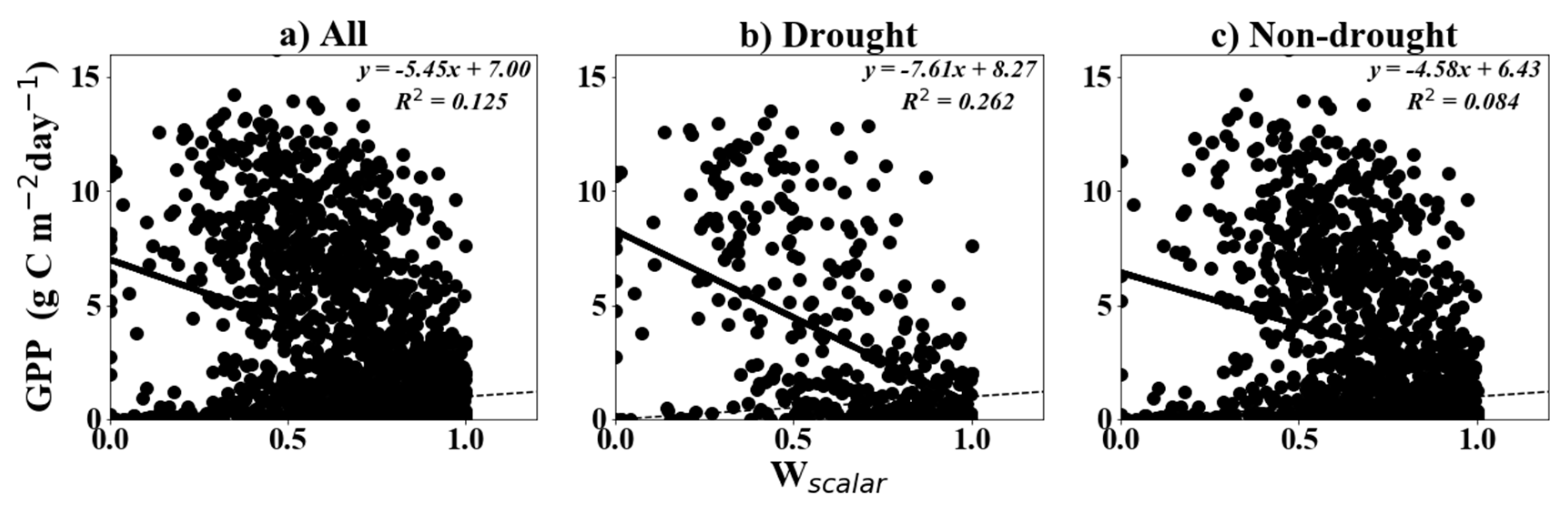
4.3. Model Performances under Drought and Non-Drought Conditions

GPPMOD could have different performances under drought conditions. We used the Standardized Precipitation Index (SPI) to identify the periods of drought. The SPI is designed to be a spatially invariant indicator of drought, which recognizes the importance of time scale in the analysis of water use [63]. In this study, the precipitation from the FluxNet sites was used to calculate SPI for each month to determine the status of drought [64]. If SPI was less than −0.5, it was defined as drought [65]. We analyzed the relationships between monthly GPPMOD and GPPEC in both non-drought and drought conditions. The results showed that GPPMOD had higher R2 (0.72 (0.66–0.79)) and lower RMSE (2.33 (2.05–2.60) g Cm−2 day−1) in drought conditions than in non-drought conditions with lower R2 (0.64 (0.61–0.68)) and higher RMSE (2.48 (2.34–2.62) g Cm−2 day−1), which indicates that GPPMOD had better explanatory capabilities for GPPEC variances under drought conditions than under non-drought conditions (Table A1).
Although several studies have reported that the standard MODIS GPP products did not accurately estimate carbon uptake during drought conditions [24,66,67]. The role of VPD in determining GPP has been examined [68]. For example, Turner et al. [46] pointed out that a high VPD scalar could reduce GPP values during a dry period. Another study also found that VPD had a weak positive correlation with GPP. Furthermore, VPD sometimes failed to capture drought events [69]. In this study, however, it is notable that GPPMOD had a better performance in drought conditions than in non-drought conditions for grasslands.
We analyzed the relationships between the VPD-based water scalar and GPPMOD and found a higher R2 between GPP and VPD-based water scaler in drought conditions (Figure 7) even though they had weak correlations in both drought and non-drought conditions (26% vs. 8%, Figure 7b,c). The MOD17A2H GPP products of grassland have better performance in drought conditions, which could be attributed to the Wscalar. However, there could be some uncertainty in the drought identification since SPI calculation was based on a short-term precipitation record in some sites. More studies are still needed in the future for a thorough analyses. The weak correlation between Wscalar and GPP suggest that the water scalar could be further improved in the grasslands.

5. Conclusions

The GPP of grassland ecosystems plays a vital role in carbon sequestration, food production, and biodiversity [70]. In this study, we investigated and evaluated the performance and robustness of GPPMOD at grassland sites across the globe. We found that: (1) GPPMOD validation at 15 global eddy covariance sites suggested a high explanation capability of GPP variances (66%) but GPPMOD generally underestimated GPP about 34% for grassland ecosystems. (2) GPPMOD performed better for the temperate grassland (R2 = 0.72 (0.68–0.75), RMSE = 2.40 (2.25–2.54) g Cm−2 day−1) than the alpine (R2 = 0.64 (0.59–0.68), RMSE = 2.55 (2.30–2.79) g Cm−2 day−1) and the tropical grasslands (R2 = 0.40 (0.27–0.52), RMSE = 2.45 (2.13–2.76) g Cm−2 day−1). The inconsistent underestimates of GPPMOD for the three grassland biomes may be rooted in the MODIS GPP algorithm, which underestimated εmax for the different grassland biomes. The varied performances of the GPP standard products in different grassland types implied that the parameterization of the MOD17A2H GPP products (e.g., εmax, FPAR, and water scalar) could be improved to better capture changes in GPP.

Author Contributions

Conceptualization, Z.X., J.D. and Z.Z.; Methodology, Z.X., Y.P. and Y.Z.; Software, Z.X., Y.P., Y.Z. and G.Z.; Validation, Z.X. and Y.P.; Formal Analysis, Y.P. and Z.X.; Data Curation, X.X.; Writing-Original Draft Preparation, Z.X.; Writing-Review & Editing, Y.P., J.D. and Z.X.; Supervision, Y.Z., J.B., L.C., R.B.D., G.Z. and X.X.

Funding

This research was funded by the Strategic Priority Research Program (XDA19040301), the Key Research Program of Frontier Sciences (QYZDB-SSW-DQC005) of the Chinese Academy of Sciences (CAS), and the “Thousand Youth Talents Plan”.

Conflicts of Interest

The authors declare no conflict of interest.

Appendix A

Table A1. The relationship between GPPEC and GPPMOD for the temperate, tropical, and alpine grassland biomes in both non-drought and drought conditions. The 95% confidence interval using the bootstrapping method is in parenthesis.
TypeSlopeR2RMSE
Drought conditionsTropical grassland1.05 (0.26, 1.85)0.37 (0.01, 0.86)3.55 (2.39, 4.49)
Temperate grassland1.22 (1.12, 1.32)0.79 (0.73, 0.85)2.14(1.86, 2.42)
Alpine grassland1.20 (1.04, 1.36)0.68 (0.57, 0.78)2.36 (1.83, 2.84)
ALL1.19(1.10, 1.28)0.72 (0.66, 0.79)2.33 (2.05, 2.60)
Non-drought conditionsTropical grassland1.01 (0.81, 1.20)0.40 (0.28, 0.54)2.31 (1.99, 2.62)
Temperate grassland1.26 (1.20, 1.32)0.70 (0.66, 0.74)2.45 (2.28, 2.61)
Alpine grassland1.26 (1.17, 1.35)0.63 (0.58, 0.68)2.59 (2.32, 2.87)
ALL1.23 (1.18, 1.28)0.65 (0.61, 0.68)2.48 (2.34, 2.62)

References

  1. Beer, C.; Reichstein, M.; Tomelleri, E.; Ciais, P.; Jung, M.; Carvalhais, N.; Rodenbeck, C.; Arain, M.A.; Baldocchi, D.; Bonan, G.B.; et al. Terrestrial Gross Carbon Dioxide Uptake: Global Distribution and Covariation with Climate. Science 2010, 329, 834–838. [Google Scholar] [CrossRef] [PubMed]
  2. Kotchenova, S.Y.; Song, X.; Shabanov, N.V.; Potter, C.S.; Knyazikhin, Y.; Myneni, R.B. Lidar Remote Sens. for modeling gross primary production of deciduous forests. Remote Sens. Environ. 2004, 92, 158–172. [Google Scholar] [CrossRef]
  3. Falge, E. Seasonality of ecosystem respiration and gross primary production as derived from FLUXNET measurements. Agric. For. Meteorol. 2002, 113, 53–74. [Google Scholar] [CrossRef] [Green Version]
  4. Zhou, L.; He, H.-L.; Sun, X.-M.; Zhang, L.; Yu, G.-R.; Ren, X.-L.; Wang, J.-Y.; Zhao, F.-H. Modeling winter wheat phenology and carbon dioxide fluxes at the ecosystem scale based on digital photography and eddy covariance data. Ecol. Inform. 2013, 18, 69–78. [Google Scholar] [CrossRef]
  5. Che, M.; Chen, B.; Innes, J.L.; Wang, G.; Dou, X.; Zhou, T.; Zhang, H.; Yan, J.; Xu, G.; Zhao, H. Spatial and temporal variations in the end date of the vegetation growing season throughout the Qinghai–Tibetan Plateau from 1982 to 2011. Agric. For. Meteorol. 2014, 189, 81–90. [Google Scholar] [CrossRef]
  6. Han, Q. Modeling the grazing effect on dry grassland carbon cycling with Biome-BGC model. Ecol. Complex. 2014, 17, 149–157. [Google Scholar] [CrossRef]
  7. Zhang, Y.; Xiao, X.; Guanter, L.; Zhou, S.; Ciais, P.; Joiner, J.; Sitch, S.; Wu, X.; Nabel, J.; Dong, J.; et al. Precipitation and carbon-water coupling jointly control the interannual variability of global land gross primary production. Sci. Rep. 2016, 6, 39748. [Google Scholar] [CrossRef] [PubMed] [Green Version]
  8. Singh, R.P.; Rovshan, S.; Goroshi, S.K.; Panigrahy, S.; Parihar, J.S. Spatial and Temporal Variability of Net Primary Productivity (NPP) over Terrestrial Biosphere of India Using NOAA-AVHRR Based GloPEM Model. J. Indian Soc. Remote Sens. 2011, 39, 345–353. [Google Scholar] [CrossRef]
  9. Yuan, J.; Niu, Z.; Wang, C. Vegetation NPP distribution based on MODIS data and CASA model—A case study of northern Hebei Province. Chin. Geogr. Sci. 2006, 16, 334–341. [Google Scholar] [CrossRef]
  10. Xiao, X.; Zhang, Q.; Saleska, S.; Hutyra, L.; De Camargo, P.; Wofsy, S.; Frolking, S.; Boles, S.; Keller, M.; Moore, B. Satellite-based modeling of gross primary production in a seasonally moist tropical evergreen forest. Remote Sens. Environ. 2005, 94, 105–122. [Google Scholar] [CrossRef]
  11. Zhang, Y.; Xiao, X.; Jin, C.; Dong, J.; Zhou, S.; Wagle, P.; Joiner, J.; Guanter, L.; Zhang, Y.; Zhang, G.; et al. Consistency between sun-induced chlorophyll fluorescence and gross primary production of vegetation in North America. Remote Sens. Environ. 2016, 183, 154–169. [Google Scholar] [CrossRef] [Green Version]
  12. Ito, A. The regional carbon budget of East Asia simulated with a terrestrial ecosystem model and validated using AsiaFlux data. Agric. For. Meteorol. 2008, 148, 738–747. [Google Scholar] [CrossRef]
  13. Malciute, A.; Naujalis, J.R.; Sauliene, I. The seasonal development characteristics of different taxa and cultivars of rhododendrons in Northern Lithuania. 2. Flowering peculiarities. Zemdirb.-Agric. 2011, 98, 81–92. [Google Scholar]
  14. Running, S.W.; Nemani, R.R.; Heinsch, F.A.; Zhao, M.S.; Reeves, M.; Hashimoto, H. A continuous satellite-derived measure of global terrestrial primary production. Bioscience 2004, 54, 547–560. [Google Scholar] [CrossRef]
  15. Wang, H.; Jia, G.; Fu, C.; Feng, J.; Zhao, T.; Ma, Z. Deriving maximal light use efficiency from coordinated flux measurements and satellite data for regional gross primary production modeling. Remote Sens. Environ. 2010, 114, 2248–2258. [Google Scholar] [CrossRef]
  16. Horn, J.E.; Schulz, K. Spatial extrapolation of light use efficiency model parameters to predict gross primary production. J. Adv. Model. Earth Syst. 2011, 3. [Google Scholar] [CrossRef] [Green Version]
  17. Yuan, W.; Cai, W.; Xia, J.; Chen, J.; Liu, S.; Dong, W.; Merbold, L.; Law, B.; Arain, A.; Beringer, J.; et al. Global comparison of light use efficiency models for simulating terrestrial vegetation gross primary production based on the LaThuile database. Agric. For. Meteorol. 2014, 192, 108–120. [Google Scholar] [CrossRef]
  18. Yuan, W.; Chen, Y.; Xia, J.; Dong, W.; Magliulo, V.; Moors, E.; Olesen, J.E.; Zhang, H. Estimating crop yield using a satellite-based light use efficiency model. Ecol. Indic. 2016, 60, 702–709. [Google Scholar] [CrossRef] [Green Version]
  19. Zhang, Y.; Xiao, X.; Zhou, S.; Ciais, P.; McCarthy, H.; Luo, Y. Canopy and physiological controls of GPP during drought and heat wave. Geophys. Res. Lett. 2016, 43, 3325–3333. [Google Scholar] [CrossRef]
  20. Zhang, Y.; Xu, M.; Chen, H.; Adams, J. Global pattern of NPP to GPP ratio derived from MODIS data: Effects of ecosystem type, geographical location and climate. Glob. Ecol. Biogeogr. 2009, 18, 280–290. [Google Scholar] [CrossRef]
  21. Xia, J.; Niu, S.; Ciais, P.; Janssens, I.A.; Chen, J.; Ammann, C.; Arain, A.; Blanken, P.D.; Cescatti, A.; Bonal, D.; et al. Joint control of terrestrial gross primary productivity by plant phenology and physiology. Proc. Natl. Acad. Sci. USA 2015, 112, 2788–2793. [Google Scholar] [CrossRef] [PubMed] [Green Version]
  22. Zhao, M.; Heinsch, F.A.; Nemani, R.R.; Running, S.W. Improvements of the MODIS terrestrial gross and net primary production global data set. Remote Sens. Environ. 2005, 95, 164–176. [Google Scholar] [CrossRef]
  23. Sims, D.; Rahman, A.; Cordova, V.; Elmasri, B.; Baldocchi, D.; Bolstad, P.; Flanagan, L.; Goldstein, A.; Hollinger, D.; Misson, L. A new model of gross primary productivity for North American ecosystems based solely on the enhanced vegetation index and land surface temperature from MODIS. Remote Sens. Environ. 2008, 112, 1633–1646. [Google Scholar] [CrossRef]
  24. Coops, N.; Black, T.; Jassal, R.; Trofymow, J.; Morgenstern, K. Comparison of MODIS, eddy covariance determined and physiologically modelled gross primary production (GPP) in a Douglas-fir forest stand. Remote Sens. Environ. 2007, 107, 385–401. [Google Scholar] [CrossRef]
  25. Turner, D.P.; Ritts, W.D.; Cohen, W.B.; Gower, S.T.; Zhao, M.; Running, S.W.; Wofsy, S.C.; Urbanski, S.; Dunn, A.L.; Munger, J.W. Scaling Gross Primary Production (GPP) over boreal and deciduous forest landscapes in support of MODIS GPP product validation. Remote Sens. Environ. 2003, 88, 256–270. [Google Scholar] [CrossRef] [Green Version]
  26. Leuning, R.; Cleugh, H.A.; Zegelin, S.J.; Hughes, D. Carbon and water fluxes over a temperate Eucalyptus forest and a tropical wet/dry savanna in Australia: Measurements and comparison with MODIS Remote Sens. estimates. Agric. For. Meteorol. 2005, 129, 151–173. [Google Scholar] [CrossRef]
  27. Sjöström, M.; Zhao, M.; Archibald, S.; Arneth, A.; Cappelaere, B.; Falk, U. Evaluation of MODIS gross primary productivity for Africa using eddy covariance data. Remote Sens. Environ. 2013, 131, 275–286. [Google Scholar] [CrossRef]
  28. Running, S.W.; Maosheng, Z. User’s Guide Daily GPP and Annual NPP (MOD17A2/A3) Products NASA Earth Observing System MODIS Land Algorithm; The Numerical Terradynamic Simulation Group: Missoula, MT, USA, 2015. [Google Scholar]
  29. Zhang, Y.; Yu, Q.; Jiang, J.I.E.; Tang, Y. Calibration of Terra/MODIS gross primary production over an irrigated cropland on the North China Plain and an alpine meadow on the Tibetan Plateau. Glob. Chang. Biol. 2008, 14, 757–767. [Google Scholar] [CrossRef] [Green Version]
  30. Zhu, H.; Lin, A.; Wang, L.; Xia, Y.; Zou, L. Evaluation of MODIS Gross Primary Production across Multiple Biomes in China Using Eddy Covariance Flux Data. Remote Sens. 2016, 8, 395. [Google Scholar] [CrossRef]
  31. Doughty, R.; Xiao, X.; Wu, X.; Zhang, Y.; Bajgain, R.; Zhou, Y.; Qin, Y.; Zou, Z.; McCarthy, H.; Friedman, J.; et al. Responses of gross primary production of grasslands and croplands under drought, pluvial, and irrigation conditions during 2010–2016, Oklahoma, USA. Agric. Water Manag. 2018, 204, 47–59. [Google Scholar] [CrossRef]
  32. Dennis Baldocchi, E.F. FLUXNET: A New Tool to Study the Temporal and Spatial Variability of Ecosystem-Scale Carbon Dioxide, Water Vapor, and Energy Flux Densities. Am. Meteorol. Soc. 2001, 82, 2415–2434. [Google Scholar] [CrossRef]
  33. Kucharik, C.J.; Barford, C.C.; Maayar, M.E.; Wofsy, S.C.; Monson, R.K.; Baldocchi, D.D. A multiyear evaluation of a Dynamic Global Vegetation Model at three AmeriFlux forest sites: Vegetation structure, phenology, soil temperature, and CO2 and H2O vapor exchange. Ecol. Model. 2006, 196, 1–31. [Google Scholar] [CrossRef]
  34. Papale, D. Effect of spatial sampling from European flux towers for estimating carbon and water fluxes with artificial neural networks. J. Geophys. Res. Biogeosci. 2015, 120, 1941–1957. [Google Scholar] [CrossRef]
  35. Fu, Y.-L. Depression of net ecosystem CO2 exchange in semi-arid Leymus chinensis steppe and alpine shrub. Agric. For. Meteorol. 2006, 137, 234–244. [Google Scholar] [CrossRef]
  36. Vuichard, N. Filling the gaps in meteorological continuous data measured at FLUXNET sites with ERA-Interim reanalysis. Earth Syst. Sci. Data 2015, 7, 157–171. [Google Scholar] [CrossRef] [Green Version]
  37. Xiao, X. Light Absorption by Leaf Chlorophyll and Maximum Light Use Efficiency. IEEE Trans. Geosci. Remote Sens. 2006, 44, 1933–1935. [Google Scholar] [CrossRef]
  38. Zhao, M.; Running, S.W. Drought-Induced Reduction in Global Terrestrial Net Primary Production from 2000 through 2009. Science 2010, 329, 940–943. [Google Scholar] [CrossRef] [PubMed]
  39. Reichstein, M. On the separation of net ecosystem exchange into assimilation and ecosystem repiration:review and improved algorithm. Glob. Chang. Biol. 2005, 11, 1424–1439. [Google Scholar] [CrossRef]
  40. Piñeiro, G.; Perelman, S.; Guerschman, J.P.; Paruelo, J.M. How to evaluate models: Observed vs. predicted or predicted vs. observed? Ecol. Model. 2008, 216, 316–322. [Google Scholar] [CrossRef]
  41. Goulden, M.L.; Daube, B.C.; Fan, S.M.; Sutton, D.J.; Bazzaz, A.; Munger, J.W.; Wofsy, S.C. Physiological responses of a black spruce forest to weather. J. Geophys. Res. Atmos. 1997, 102, 28987–28996. [Google Scholar] [CrossRef] [Green Version]
  42. Xiao, X.M.; Hollinger, D.; Aber, J.; Goltz, M.; Davidson, E.A.; Zhang, Q.Y.; Moore, B. Satellite-based modeling of gross primary production in an evergreen needleleaf forest. Remote Sens. Environ. 2004, 89, 519–534. [Google Scholar] [CrossRef]
  43. Frolking, S.E.; Bubier, J.L.; Moore, T.R.; Ball, T.; Bellisario, L.M.; Bhardwaj, A.; Carroll, P.; Crill, P.M.; Lafleur, P.M.; Mccaughey, J.H. Relationship between ecosystem productivity and photosynthetically active radiation for northern peatlands. Glob. Biogeochem. Cycles 1998, 12, 115–126. [Google Scholar] [CrossRef] [Green Version]
  44. Ruimy, A.; Dedieu, G.; Saugier, B. TURC: A diagnostic model of continental gross primary productivity and net primary productivity. Glob. Biogeochem. Cycles 1996, 10, 269–285. [Google Scholar] [CrossRef]
  45. Ruimy, A.; Jarvis, P.G.; Baldocchi, D.D.; Saugier, B. CO2 Fluxes over Plant Canopies and Solar Radiation: A Review. Adv. Ecol. Res. 1995, 26, 1–68. [Google Scholar]
  46. Turner, D.P.; Ritts, W.D.; Cohen, W.B.; Maeirsperger, T.K.; Gower, S.T.; Kirschbaum, A.A.; Running, S.W.; Zhao, M.; Wofsy, S.C.; Dunn, A.L.; et al. Site-level evaluation of satellite-based global terrestrial gross primary production and net primary production monitoring. Glob. Chang. Biol. 2005, 11, 666–684. [Google Scholar] [CrossRef]
  47. Xiao, J.; Zhuang, Q.; Law, B.E.; Chen, J.; Baldocchi, D.D.; Cook, D.R.; Oren, R.; Richardson, A.D.; Wharton, S.; Ma, S.; et al. A continuous measure of gross primary production for the conterminous United States derived from MODIS and AmeriFlux data. Remote Sens. Environ. 2010, 114, 576–591. [Google Scholar] [CrossRef]
  48. Wu, C.; Chen, J.M.; Huang, N. Predicting gross primary production from the enhanced vegetation index and photosynthetically active radiation: Evaluation and calibration. Remote Sens. Environ. 2011, 115, 3424–3435. [Google Scholar] [CrossRef]
  49. Gu, Y.; Wylie, B.K.; Bliss, N.B. Mapping grassland productivity with 250-m eMODIS NDVI and SSURGO database over the Greater Platte River Basin, USA. Ecol. Indic. 2013, 24, 31–36. [Google Scholar] [CrossRef]
  50. Propastin, P.; Ibrom, A.; Knohl, A.; Erasmi, S. Effects of canopy photosynthesis saturation on the estimation of gross primary productivity from MODIS data in a tropical forest. Remote Sens. Environ. 2012, 121, 252–260. [Google Scholar] [CrossRef]
  51. Wu, W.; Wang, S.; Xiao, X.; Yu, G.; Fu, Y.; Hao, Y. Modeling gross primary production of a temperate grassland ecosystem in Inner Mongolia, China, using MODIS imagery and climate data. Sci. China Ser. D Earth Sci. 2008, 51, 1501–1512. [Google Scholar] [CrossRef]
  52. Wang, X.; Ma, M.; Huang, G.; Veroustraete, F.; Zhang, Z.; Song, Y.; Tan, J. Vegetation primary production estimation at maize and alpine meadow over the Heihe River Basin, China. Int. J. Appl. Earth Obs. Geoinf. 2012, 17, 94–101. [Google Scholar] [CrossRef]
  53. Zhou, Y.; Zhang, L.; Xiao, J.; Chen, S.; Kato, T.; Zhou, G. A Comparison of Satellite-Derived Vegetation Indices for Approximating Gross Primary Productivity of Grasslands. Rangel. Ecol. Manag. 2014, 67, 9–18. [Google Scholar] [CrossRef]
  54. Zhang, Y.; Xiao, X.; Wolf, S.; Wu, J.; Wu, X.; Gioli, B.; Wohlfahrt, G.; Cescatti, A.; van der Tol, C.; Zhou, S.; et al. Spatio-temporal Convergence of Maximum Daily Light-Use Efficiency Based on Radiation Absorption by Canopy Chlorophyll. Geophys. Res. Lett. 2018, 45, 3508–3519. [Google Scholar] [CrossRef]
  55. Liu, Z.; Wu, C.; Peng, D.; Wang, S.; Gonsamo, A.; Fang, B.; Yuan, W. Improved modeling of gross primary production from a better representation of photosynthetic components in vegetation canopy. Agric. For. Meteorol. 2017, 233, 222–234. [Google Scholar] [CrossRef]
  56. Li, F.; Wang, X.F.; Zhao, J.; Zhang, X.Q.; Zhao, Q.J. A method for estimating the gross primary production of alpine meadows using MODIS and climate data in China. Int. J. Remote Sens. 2013, 34, 8280–8300. [Google Scholar] [CrossRef]
  57. Goulden, S.D. Diel and seasonal patterns of tropical forest CO2-exchange. Ecol. Appl. 2004, 14, 542–554. [Google Scholar] [CrossRef]
  58. Turner, D.P.; Ritts, W.D.; Cohen, W.B.; Gower, S.T.; Running, S.W.; Zhao, M.; Costa, M.H.; Kirschbaum, A.A.; Ham, J.M.; Saleska, S.R.; et al. Evaluation of MODIS NPP and GPP products across multiple biomes. Remote Sens. Environ. 2006, 102, 282–292. [Google Scholar] [CrossRef]
  59. Lagergren, F. Net primary production and light use efficiency in a mixed coniferous forest in Sweden. Plant Cell Environ. 2005, 28, 412–423. [Google Scholar] [CrossRef] [Green Version]
  60. Zhang, Y. A global moderate resolution dataset of gross primary production of vegetation for 2000–2016. Sci. Data 2017, 4, 170165. [Google Scholar] [CrossRef] [PubMed]
  61. Dong, J.W.; Xiao, X.M.; Wagle, P.; Zhang, G.L.; Zhou, Y.T.; Jin, C.; Torn, M.S.; Meyers, T.P.; Suyker, A.E.; Wang, J.B.; et al. Comparison of four EVI-based models for estimating gross primary production of maize and soybean croplands and tallgrass prairie under severe drought. Remote Sens. Environ. 2015, 162, 154–168. [Google Scholar] [CrossRef] [Green Version]
  62. Yi, Y.; Kimball, J.S.; Jones, L.A.; Reichle, R.H.; McDonald, K.C. Evaluation of MERRA land surface estimates in preparation for the soil moisture active passive mission. J. Clim. 2011, 24, 3797–3816. [Google Scholar] [CrossRef]
  63. Guttman, N.B. Accepting the Standardized Precipitation Index: A Calculation Algorithm. Jawra J. Am. Water Resour. Assoc. 2010, 35, 311–322. [Google Scholar] [CrossRef]
  64. Seiler, R.A.; Hayes, M.; Bressan, L. Using the standardized precipitation index for flood risk monitoring. Int. J. Climatol. 2002, 22, 1365–1376. [Google Scholar] [CrossRef] [Green Version]
  65. Tao, X.e.; Chen, H.; Xu, C. Characteristics of drought variations in Hanjiang Basin in 1961-2014 based on SPI/SPEI. J. Water Resour. Res. 2015, 4, 404. [Google Scholar] [CrossRef]
  66. Zhang, L.; Wylie, B.; Loveland, T.; Fosnight, E.; Tieszen, L.L.; Ji, L.; Gilmanov, T. Evaluation and comparison of gross primary production estimates for the Northern Great Plains grasslands. Remote Sens. Environ. 2007, 106, 173–189. [Google Scholar] [CrossRef] [Green Version]
  67. Hwang, T.; Kang, S.; Kim, J.; Kim, Y.; Lee, D.; Band, L. Evaluating drought effect on MODIS Gross Primary Production (GPP) with an eco-hydrological model in the mountainous forest, East Asia. Glob. Chang. Biol. 2008, 14, 1037–1056. [Google Scholar] [CrossRef]
  68. Akmal, M.; Janssens, M.J.J. Productivity and light use efficiency of perennial ryegrass with contrasting water and nitrogen supplies. Field Crops Res. 2004, 88, 143–155. [Google Scholar] [CrossRef]
  69. Hashimoto, H.; Wang, W.; Milesi, C.; Xiong, J.; Ganguly, S.; Zhu, Z.; Nemani, R. Structural Uncertainty in Model-Simulated Trends of Global Gross Primary Production. Remote Sens. 2013, 5, 1258–1273. [Google Scholar] [CrossRef]
  70. Lee, M.; Manning, P.; Rist, J.; Power, S.A.; Marsh, C. A global comparison of grassland biomass responses to CO2 and nitrogen enrichment. Philos. Trans. R. Soc. Lond. B 2010, 365, 2047–2056. [Google Scholar] [CrossRef] [PubMed]
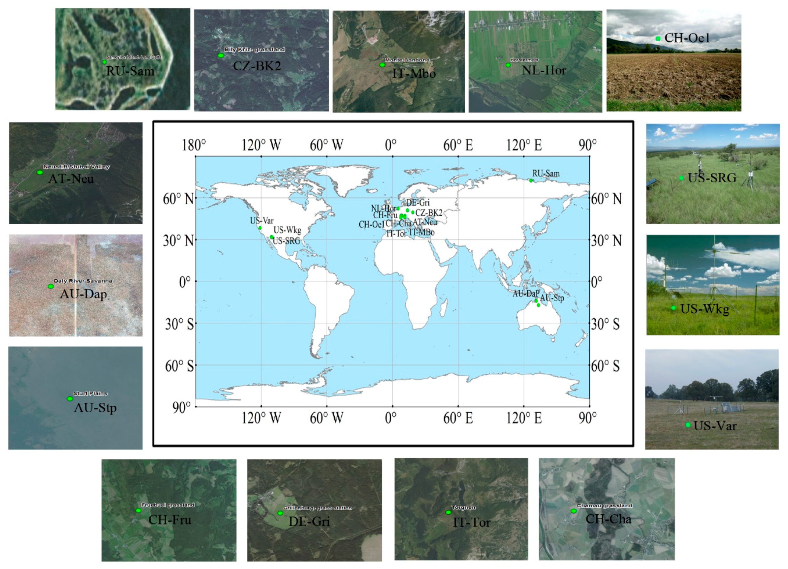
Figure 1. Distribution of 15 FLUXNET sites selected with more than five years of observations.
Remotesensing 10 01771 g001
Figure 2. Seasonal variations of GPPMOD and observed GPPEC at all study sites.
Remotesensing 10 01771 g002
Figure 3. The relationship between GPPMOD and GPPEC for all sites. The short-dashed line is a 1:1 line. The unit of RMSE was g C m−2 day−1.
Remotesensing 10 01771 g003
Figure 4. The relationship between GPPMOD and GPPEC for all sites. The short-dashed line is a 1:1 line. The unit of RMSE was g C m−2 day−1.
Remotesensing 10 01771 g004
Figure 5. The relationships between GPPEC and GPPMOD for the temperate, tropical, and alpine grassland biomes. The short-dashed line is a 1:1 line. The unit of RMSE was g C m−2 day−1.
Remotesensing 10 01771 g005
Figure 6. The relationship between GPPMOD and GPPEC for all sites with the εmax ( ε m a x -BPLUT) used in the MOD17 GPP algorithm was replaced by the estimated εmax ( ε m a x -EST). The unit of RMSE was g C m−2 day−1.
Remotesensing 10 01771 g006
Figure 7. The relationships between Wscalar of MOD17A2H GPP products and GPPEC, respectively. The solid line is a linear regression. The short-dashed line is a 1:1 line.
Remotesensing 10 01771 g007
Table 1. Basic information of FLUXNET eddy covariance tower sites selected in this study.
Site IDSite NameLATLONIGBP ClassData Range
CH-ChaChamau47.21028.4104Temperate grassland2005–2014
CH-FruFruebuel grassland47.11588.5378Temperate grassland2005–2014
CH-Oe1Oensingen grassland47.28587.7319Temperate grassland2002–2008
DE-GriGrillenburg50.949513.5125Temperate grassland2004–2014
NL-HorHorstermeer52.24045.0713Temperate grassland2004–2011
US-SRGSanta Rita Grasslan31.7894−110.8277Temperate grassland2008–2014
US-WkgWalnut Gulch Kendall grasslands31.7365−109.9419Temperate grassland2004–2014
AU-DapDaly River avanna−14.0633131.3181Tropical grassland2007–2013
AU-StpSturt Plains−17.1507133.3502Tropical grassland2008–2014
US-VarVaira Ranch-Ione38.4133−120.9507Tropical grassland2001–2014
AT-NeuNeustift47.116711.3175Alpine grassland2002–2012
CZ-Bk2Bily Kriz grassland49.494418.5429Alpine grassland2006–2012
IT-MboMonte Bondone46.014711.0458Alpine grassland2003–2013
RU-SamSamoylov72.3733126.4978Alpine grassland2002–2014
IT-TorTorgnon45.84447.5781Alpine grassland2008–2014
Table 2. Statistics of the comparison between monthly GPPMOD and GPPEC for all sites by using the linear regression model. The 95% confidence interval using the bootstrapping method is in parenthesis.
Site IDSlopeR2RMSE
AT-Neu1.89 (1.72, 2.07)0.78 (0.72, 0.83)4.05 (3.52, 4.55)
AU-Dap0.92 (0.60, 1.24)0.28 (0.14, 0.45)3.31 (2.88, 3.70)
AU-Stp0.89 (0.70, 1.07)0.53 (0.34, 0.70)1.04 (0.83, 1.24)
CH-Cha1.14 (1.03, 1.25)0.79 (0.70, 0.86)3.64 (3.29, 4.00)
CH-Fru1.27 (1.14, 1.39)0.78 (0.71, 0.84)3.19 (2.78, 3.57)
CH-Oe11.14 (0.94, 1.34)0.61 (0.48, 0.74)3.19 (2.72, 3.66)
CZ-Bk21.04 (0.93, 1.15)0.82 (0.74, 0.88)1.31 (1.05, 1.54)
DE-Gri1.15 (1.06, 1.24)0.83 (0.77, 0.89)1.90 (1.61, 2.18)
IT-Mbo1.05 (0.92, 1.18)0.67 (0.57, 0.76)2.36 (1.87, 2.82)
IT-Tor1.30 (1.01, 1.58)0.50 (0.33, 0.67)2.81 (2.23, 3.34)
NL-Hor0.86 (0.71, 1.00)0.59 (0.48, 0.68)2.05 (1.72, 2.36)
RU-Sam0.58 (0.37, 0.79)0.17 (0.08, 0.29)0.89 (0.74, 1.03)
US-SRG0.50 (0.37, 0.63)0.40 (0.18, 0.59)0.68 (0.58, 0.77)
US-Var0.91 (0.76, 1.07)0.63 (0.46, 0.76)1.72 (1.47, 1.97)
US-Wkg1.59 (1.41, 1.77)0.70 (0.61, 0.78)0.63 (0.49, 0.75)
ALL1.22 (1.18, 1.26)0.66 (0.63, 0.69)2.46 (2.33, 2.58)
Table 3. Statistics regarding the comparison between GPPEC and GPPMOD for temperate, tropical, and alpine grassland biomes using a linear regression model. The 95% confidence interval derived by the bootstrapping method is in parenthesis.
Grass TypeSlopeR2RMSE
Tropical grassland1.02 (0.83, 1.21)0.40 (0.27, 0.52)2.45 (2.13, 2.76)
Temperate grassland1.25 (1.19, 1.30)0.72 (0.68, 0.75)2.40 (2.25, 2.54)
Alpine grassland1.24 (1.17, 1.32)0.64 (0.59, 0.68)2.55 (2.30, 2.79)
Table 4. The comparison of the ε m a x between the estimated values based on the nonlinear model ( ε m a x -EST) and the values in the biome properties look-up table ( ε m a x -BPLUT) used in the MOD17 GPP algorithm. “RMSE after” and “RMSE before” referred to the RMSE between the GPPEC and GPPMOD with ε m a x -EST and ε m a x -BPLUT, respectively.
Site ID ε m a x -EST ε m a x -BPLUTRMSE AfterRMSE Before ε m a x bias
g C/MJg C/MJg Cm−2 day−1g Cm−2 day−1g C/MJ
AT-Neu1.710.862.304.050.85
AU-Dap0.870.863.303.310.01
AU-Stp0.730.860.981.04−0.13
CH_Cha0.970.863.193.640.11
CH-Fru1.280.862.243.190.42
CH-Oe11.130.862.643.190.27
CZ-Bk22.570.867.421.311.71
DE-Gri1.090.861.531.900.23
IT-Mbo0.980.862.242.360.12
IT-Tor1.130.862.552.810.27
NL-Hor0.930.862.042.050.07
RU-Sam0.930.860.890.890.07
US-SRG0.770.860.570.68−0.09
US-Var0.760.861.521.72−0.10
US-Wkg1.070.860.600.630.21

