Assessing Impacts of Urban Form on Landscape Structure of Urban Green Spaces in China Using Landsat Images Based on Google Earth Engine


1
Ministry of Education Key Laboratory for Earth System Modeling, Department of Earth System Science, Tsinghua University, Beijing 100084, China
2
Joint Center for Global Change Studies, Beijing 100875, China
*
Author to whom correspondence should be addressed.
Remote Sens. 2018, 10(10), 1569; https://doi.org/10.3390/rs10101569
Submission received: 11 August 2018
/
Revised: 25 September 2018
/
Accepted: 28 September 2018
/
Published: 1 October 2018
(This article belongs to the Special Issue Remote Sensing of Urban Ecology and Sustainability)
Abstract
:The structure of urban green spaces (UGS) plays an important role in determining the ecosystem services that they support. Knowledge of factors shaping landscape structure of UGS is imperative for planning and management of UGS. In this study, we assessed the influence of urban form on the structure of UGS in 262 cities in China based on remote sensing data. We produced land cover maps for 262 cities in 2015 using 6673 scenes of Landsat ETM+/OLI images based on the Google Earth Engine platform. We analyzed the impact of urban form on landscape structure of UGS in these cities using boosted regression tree analysis with the landscape and urban form metrics derived from the land cover maps as response and prediction variables, respectively. The results showed that the three urban form metrics—perimeter area ratio, road density, and compound terrain complexity index—were all significantly correlated with selected landscape metrics of UGS. Cities with high road density had less UGS area and the UGS in those cities was more fragmented. Cities with complex built-up boundaries tended to have more fragmented UGS. Cities with high terrain complexity had more UGS but the UGS were more fragmented. Our results for the first time revealed the importance of urban form on shaping landscape structure of UGS in 262 cities at a national scale.

1. Introduction
Urban green spaces (UGS) contribute significantly to quality of life [1,2] and sustainable development in cities [3] because they can deliver multiple ecosystem services to urban inhabitants [4,5]. UGS can regulate climate [6,7,8], remove air pollution [9], reduce stormwater run-off [10], provide recreational opportunities [5], and improve public health [11]. For example, the urban forest in Beijing could remove 772 tons of particulate matters annually [9]. In UK, urban inhabitants were found to have lower mental distresses and higher wellbeing in places with more UGS coverage [11]. Extensive studies have shown that landscape structure of UGS is closely related to ecosystem services that they can deliver [12,13,14,15]. For example, clustered UGS were found to enhance local cooling while dispersed UGS can achieve larger overall regional cooling [13]. Carbon densities were found to be strongly and positively related to the total tree cover and the proportion of tree cover in the surrounding areas [14]. Patch sizes and corridors of UGS were found to have strong positive effects on biodiversity [16]. Loss and fragmentation of UGS were found to cause declines in bird species richness [15]. Therefore, understanding the pattern of landscape structure of UGS and its shaping forces is important for urban ecosystem service management.
Remote sensing techniques have been widely used to investigate landscape structure of UGS. For example, at the single city scale, changes of landscape structure of UGS have been quantified for Jinan, China [17], Shenzhen, China [18], Hong Kong, China [19], and Hanoi, Vietnam [20] using medium (e.g., Landsat) or high resolution (e.g., Quickbird) satellite images. Spatiotemporal patterns of UGS of nine Chinese cities were investigated using ALOS, SPOT, and Landsat images [21]. The results showed that UGS in these cities were highly fragmented and dynamic. At the regional scale, landscape structure of UGS of 111 Southeast Asian cities was investigated using Landsat images and considerable variation of UGS among these cities was identified [22]. Landscape structure of urban vegetation of 100 cities around the world was quantified using Landsat images and varied percentage of urban vegetation, and different degrees of fragmentation were found for these cities [23]. So far, the majority of studies focused at single city scale and studies of large spatial scales are still limited, especially for countries and regions that are experiencing rapid urbanization such as China [24]. This might be due to the fact that obtaining landscape structure of UGS at large spatial scales using the traditional remote sensing data processing tools is labor-intensive and time-consuming. Recently, the emergence of high-performance cloud platforms like Google Earth Engine (GEE) [25] makes it possible to process massive remote sensing data more efficiently [26,27,28], and provides opportunities to study the general pattern and driving mechanism of landscape structure of UGS at large spatial scales.
Except for limited studies on landscape structure of UGS at large spatial scales, our knowledge on shaping factors of landscape structure of UGS are also limited. Existing studies have shown that cities with higher population densities tend to have smaller [22,23] and more fragmented UGS [23]. In Southeast Asia, rich cities have more UGS than poor cities [22]. Within cities, unequal economic development leads to more fragmented urban vegetation [23]. Megacities with lower annual mean temperature and higher annual precipitation were found to have more UGS relative to other large cities [28]. Apart from these climatic and socioeconomic factors, there are indications that urban form (i.e., spatial configuration of fixed elements within a city [29]) may have important influences on landscape structure of UGS. For example, a negative relationship between the extent of UGS and total length of the road network has been identified in Sheffield, UK [30]. Terrain roughness was found to be positively correlated with levels of tree canopy in Cincinnati, USA [31]. However, very few studies addressed the impact of urban form on landscape structure of UGS, especially at a large spatial scale. How urban form can affect landscape structure of UGS is still an open question.
In this study, we assessed the impact of urban form on landscape structure of UGS through a case study in China. We selected 262 Chinese cities (population >500,000) as our study sites. With information on landscape structure of UGS and urban form extracted out from Landsat images using the GEE platform, we intend to answer the following questions. What are features of landscape structure of UGS in these cities? How does the urban form of these cities affect landscape structure of UGS in these cities? Specifically, how does landscape structure of UGS vary with topography, road density, and boundary complexity?
2. Materials and Methods
2.1. Study Area
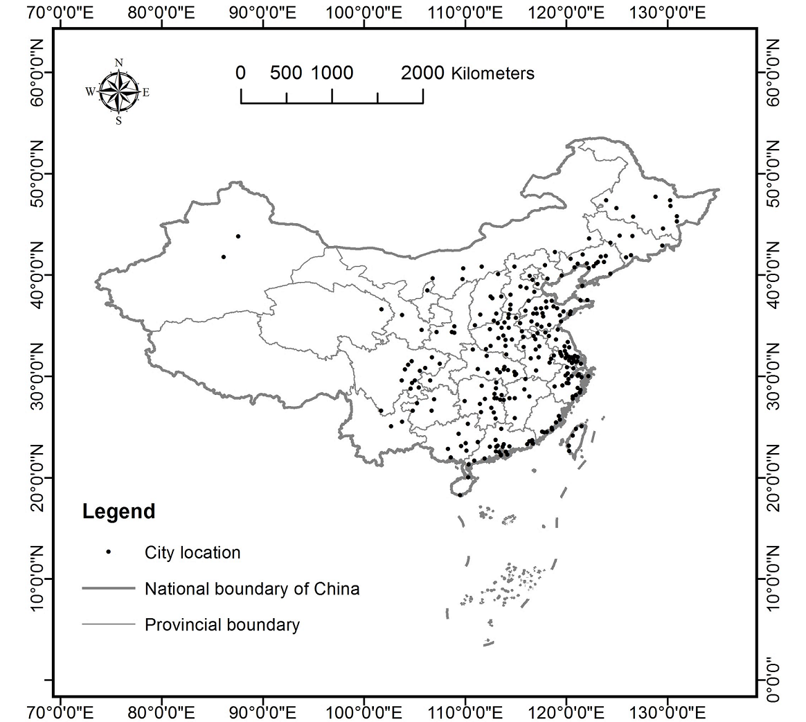
We selected 262 cities in China that had an urban population of more than 500,000 by 2014 (Figure 1, Table S1, Supplementary file 1). In total, these 262 cities accounted for 59% of China’s urban population [32]. Most of these cities are located in east China while a few cities are located in west China.
2.2. Landsat Image Processing on GEE Platform
We used 3921 scenes of standard terrain corrected (L1T) Landsat 7 ETM+ and 8 OLI/TIRS imagery with a cloud cover <70% acquired in 2015. Winter images were not used as we mainly focused on the growing season. We also included 2752 images acquired in 2014 and 2016 for 63 cities where cloud contamination was severe. The Landsat data format is the atmospherically corrected surface reflectance Landsat Collection 1 Level-1 data, which is produced by the United States Geological Survey (USGS/EROS). All images were hosted on GEE. We used the pixel_qa band of the Landsat images to mask the cloud, cloud shadow, and snow pixels [33,34,35].
We selected the blue, green, red, near infrared, and two shortwave infrared bands of Landsat images for further processing [28]. We calculated the normalized difference vegetation index (NDVI) [36], normalized difference built-up index (NDBI) [37], and modified normalized difference water index (MNDWI) [38] to enhance the information on vegetation, impervious surface, and water [28]. These calculated bands were combined with the original six bands.
We used greenest pixel compositing method [27] and percentile-based image compositing method [39] to create composited images. The greenest pixel compositing method considers associated NDVI band of each Landsat scene and selects band values from Landsat scenes that have the highest NDVI values [27]. This procedure generated a nine-band composite image for each city. For each pixel, values of NDVI and other eight bands were extracted from the same image. The percentile-based image compositing method is also a pixel-based compositing method [28]. This method first ranks all available pixel values from minimum to maximum for each specific pixel location. Then values for specific percentile can be selected. For example, value of percentile 0 represents the minimum value for a specific pixel from all available pixel values. In this study, we chose percentile values at 0%, 10%, 25%, 50%, 75%, 90%, and 100% [39] for each band. This step generated a 63-band (nine bands multiplied by seven percentile values) composite image for each city.
Images generated using the greenest pixel compositing method reflect the status of the peak growing season and were used to separate vegetation from nonvegetation. The percentile-based compositing method can capture phenology information without any explicit assumption and prior knowledge of the timing of phenology [40]. It was used to differentiate different vegetation types such as crops and grasses.
2.3. Land Cover Classification
To collect training samples, we first divided the 262 cities into three city groups according to the ‘urban ecoregions’ proposed by Schneider et al. (2010) [41]. The three city groups were Arid, semi-arid steppe in Central Asia, temperate forest in East Asia, and tropical, subtropical forest in Asia. Then we collected representative training samples of six types of land covers (i.e., water, impervious surface, bare soil, tree/shrub, grass, and crop) by referencing to high-resolution images on Google Earth (GE) [28]. We collected 500 to 5000 polygons for each class in each city group. In total, we collected 41,281 polygons as training samples. Specifically, 4900 polygons of bare soil, 6401 polygons of crop, 4319 polygons of grass, 13,073 polygons of impervious surface, 9838 polygons of tree/shrub, and 2750 polygons of water samples were collected.
We performed land cover classification on the GEE platform using the composited images, training samples, and a Random Forest (RF) classifier [42]. We first classified the percentile-based composited images into water and nonwater type. Then we classified the nonwater type into vegetation and nonvegetation type using the greenest pixel composited images. We further classified the vegetation class into tree/shrub, grass, and crop, and classified the nonvegetation type into impervious surface, and bare soil using the percentile-based composited images. The number of trees for RF was set to 100.
We conducted accuracy assessment by extracting 100 pixels for each city from the classified land cover maps as validation samples by using a stratified random sampling method [43]. The land cover classes were used as strata and the number of pixels sampled for each stratum was in proportion to the percentage of each land cover class [28]. We manually interpreted these validation samples by referencing to high-resolution images on GE and estimated classification accuracies based on the interpretation results.
2.4. UGS Extraction
Based on the land cover maps, we generated borders of urban areas for each city. We first created 1 km by 1 km impervious surface intensity (0–1) maps using the Block Statistics tool in ArcMap 10.1 (Esri Inc., Redlands, CA, USA). Next we divided the intensity maps into built/nonbuilt maps using a threshold value of 0.2 [44]. Then we converted the built/nonbuilt maps to polygons and chose the largest polygon as the core urban area of each city. We filled holes within the largest polygon using Eliminate tool in ArcMap 10.1 to form the continuous boundary of urban area. We extracted out tree/shrub and grass cover within the boundary of urban area and merged them as UGS.
2.5. Calculation of Landscape Structure Metrics
To evaluate landscape structure of UGS for each city, we calculated five landscape metrics commonly used in describing landscape structure of UGS [17,19,20,45,46]. The five landscape metrics were percentage of landscape (PLAND), patch density (PD), largest patch index (LPI), mean Euclidian nearest neighbor distance (ENN_MN), and mean patch shape index (SHAPE_MN) (Table 1). PLAND was used to quantify abundance of UGS. Cities with larger PLAND values have more UGS. LPI was used to measure dominance of UGS in the landscape. Large LPI values mean that the largest urban green space patch is more dominant in cities. PD was used to quantify the fragmentation of UGS. Cities with larger PD values have more fragmented UGS. ENN_MN was used to quantify isolation of urban green space patches. Cities with larger ENN_MN values have more dispersed UGS. SHAPE_MN was used to measure complexity of patch shapes of UGS. Cities with higher SHAPE_MN values have more complex UGS patch shapes. We calculated the landscape metrics using Fragstats 4.2 and the extracted maps of UGS [47]. We examined the correlations between these metrics using the Pearson correlation test and found they were not highly correlated with each other (R < 0.6) (Table S2).
2.6. Calculation of Urban form Metrics
We chose three commonly used urban form metrics: compound terrain complexity index (CTCI) [48,49], road density (RD) [50], and perimeter-area ratio (PARA) [45]. CTCI indicates terrain complexity of each city. It was calculated using the 30-m Shuttle Radar Topography Mission (SRTM) data [51]. CTCI was calculated as follows.
where and represent normalized standard deviation of elevation, normalized range of elevation, normalized terrain curvature, and normalized rugosity. The normalized index ( and ) was calculated as follows,
RD represents density dimension of urban form for each city, which was calculated using the road vector data downloaded from the OpenStreetMap (OSM) website (www.openstreetmap.org). The OSM is developed as a volunteered geographic information project thus the data set may include uncertainties. However, it is the most comprehensive data set on urban roads around the world that is freely available to us. RD was calculated as follows.
where L represents total length of roads, Aurban represents the size of urban area.
PARA represents shape complexity of each urban area, which was calculated using the vector boundary of continuous urban area.
where Purban represents perimeter of an urban area, Aurban represents total area of an urban area.
2.7. Statistical Analysis
Associations between landscape metrics and urban form metrics were explored using the maximal information-based nonparametric exploration (MINE) method [52]. We calculated the maximum information coefficients (MIC), Pearson correlation coefficients (ρ), and the nonlinearity coefficients (MIC-ρ2) between each landscape metric and the urban form metrics using the Java version of the MINE application [52]. The MIC values are between 0 and 1, with values near 0 representing statistically independent relationship and values near 1 representing noiseless functional relationships [52]. The MIC-ρ2 values range from 0 to 1, with values near 0 representing linear relationships and large (usually >0.2) values representing nonlinear relationships [52].
We used the boosted regression tree (BRT) model to analyze the relative importance of urban form metrics on each landscape metric. We chose the BRT model because it can handle nonlinearities and different type of variables. The BRT model was fitted using the gbm.step function of dismo package with R (version 3.3.1; R Development Core Team, Vienna, Austria). Model parameters of the learning rate, tree complexity, and bag fraction were set to 0.001, 6, and 0.75, respectively.
3. Results
3.1. Landscape Structure of UGS in 262 Chinese Cities
The mean overall classification accuracy of land cover was 88.76 ± 3.17%. The mean kappa coefficient was 0.84 ± 0.05. Confusion matrix of land cover classification for each city was listed in Supplementary file 2.
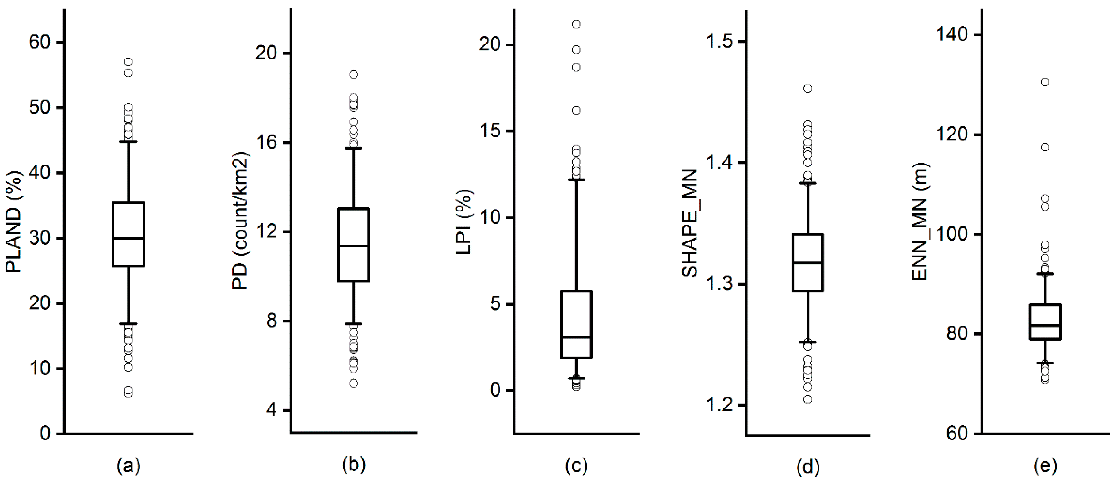
Landscape metrics of UGS for the 262 Chinese cities were shown in Figure 2. Values of the landscape metrics varied among these cities. The ENN_MN values varied from 70.73 m to 130.53 m, averaging 82.74 m (SD = 6.54 m), which showed varied dispersion of UGS patches in these cities. The mean LPI was 4.34% (SD = 3.62%), ranging from 0.22% to 21.18%. The values suggested that the dominance of the largest UGS patches is weak in most cities and variation is high among these cities. The mean SHAPE_MN was 1.32 (SD = 0.04), ranging from 1.20 to 1.46. The shape complexity of UGS did not vary much across cities. The mean PD was 11.49 count/km2 (SD = 2.48 count/km2), ranging from 5.21 to 19.06 count/km2. This wide range of PD values indicated that levels of fragmentation of UGS varied greatly in studied cities. The mean PLAND was 30.46% (SD = 8.11%), ranging from 6.17% to 57.05% (Figure 2). Clearly, abundance of UGS varied substantially among these cities.
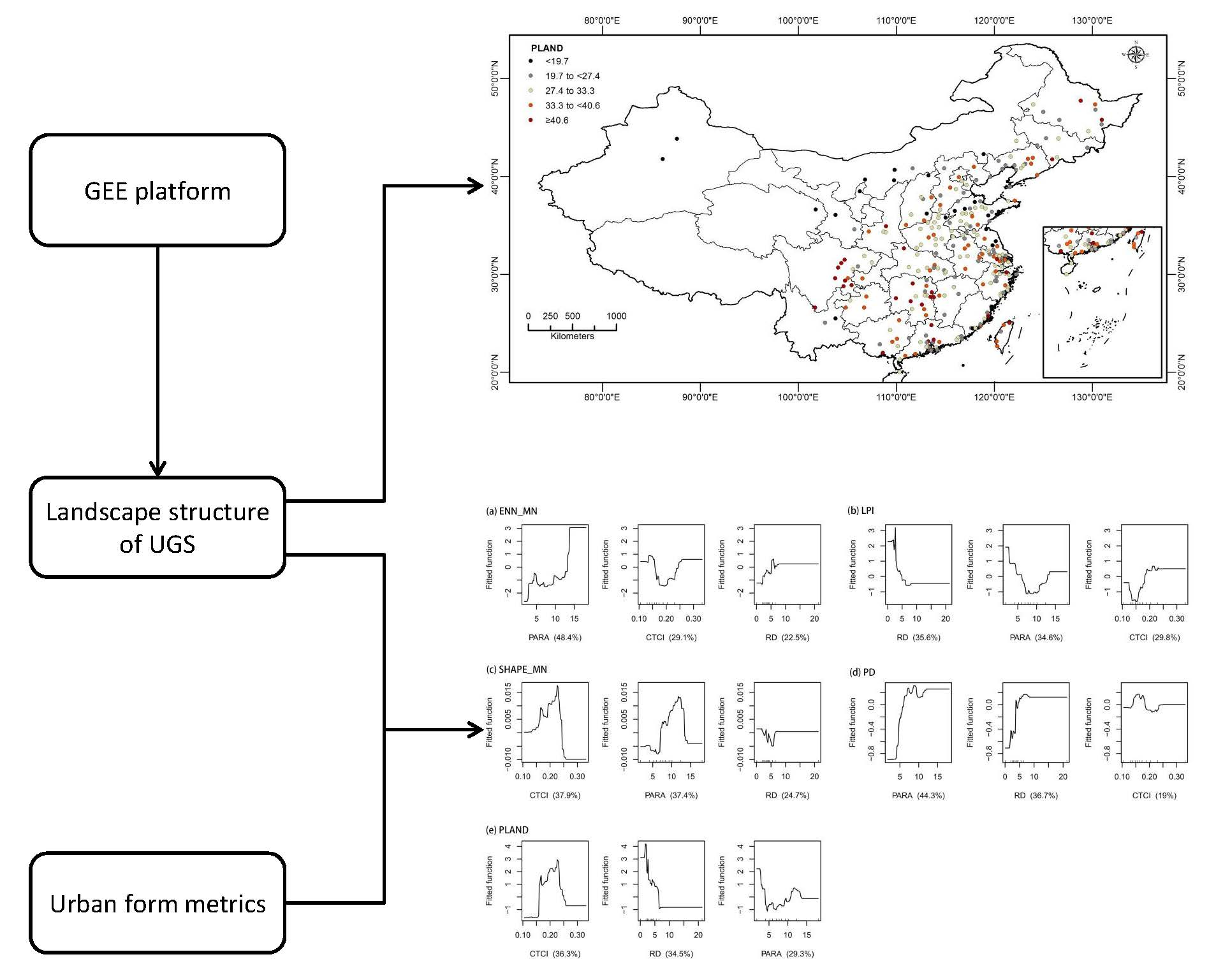
Figure 3 shows the spatial distribution of PLAND values for the 262 Chinese cities. Cities in Southwest and Central South of China had high PLAND values, which indicated that cities in these regions had high UGS coverage. However, cities in Northwestern China and North China had lower PLAND values than many other cities, which indicated that these cities had low UGS coverage (Figure 3). Spatial distributions of other four landscape metrics can be found in the supplementary file (Figures S1–S4).
3.2. Associations between Urban form Metrics and Landscape Metrics of UGS
Based on the result of MINE analysis (Table 2), CTCI was significantly correlated with SHAPE_MN and PD (p < 0.05). PARA was significantly correlated with ENN_MN and SHAPE_MN (p < 0.05). RD was significantly correlated with LPI (p < 0.05). According to the results of linear correlation, CTCI was linearly and significantly correlated with LPI and PLAND (p < 0.05). PARA was linearly and significantly correlated with ENN_MN, SHAPE_MN, and PD (p < 0.05). RD was linearly and significantly correlated with ENN_MN, LPI, and PLAND (p < 0.05) (Table 2). These results indicated that urban form metrics have significant influences on landscape structure of UGS.
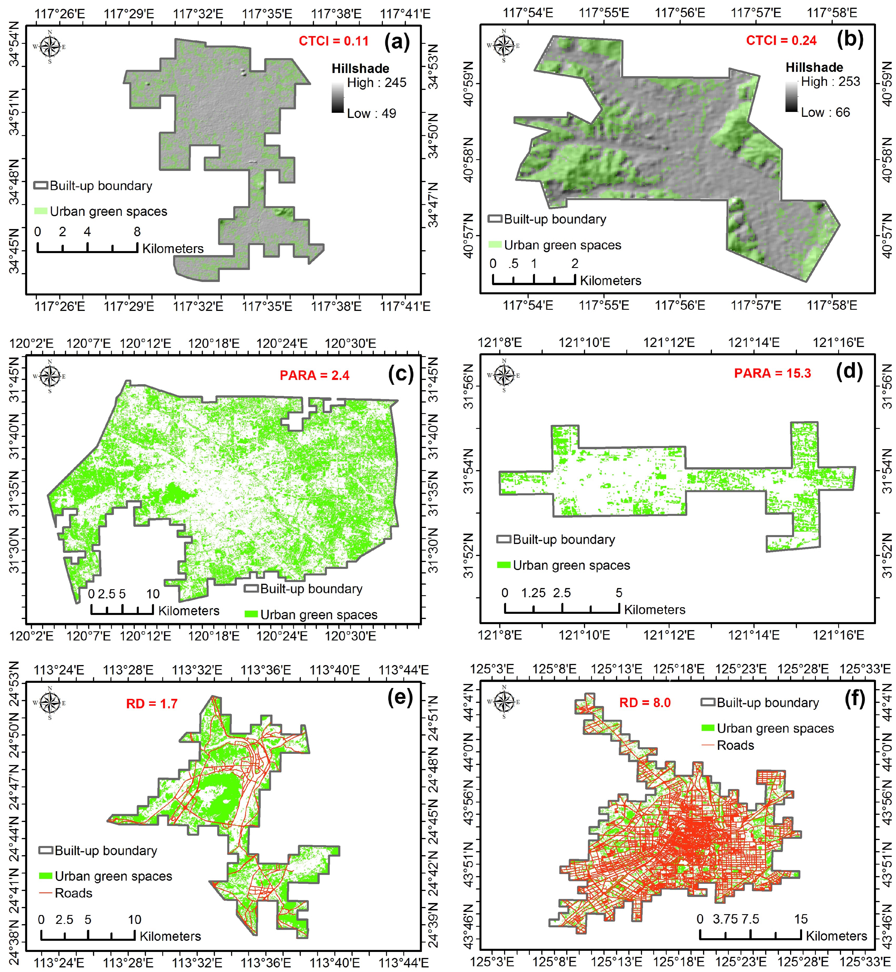
The close relationship between urban form and landscape structure can be seen from some examples (Figure 4). Chengde, Hebei (CTCI = 0.24) had a more complex terrain than Zaozhuang, Shandong (CTCI = 0.11) (Figure 4a,b). It had more UGS (PLAND = 37.5%) than Zaozhuang (PLAND = 26.6%), but UGS in Chengde (PD = 13.1 count/km2) were more fragmented than that in Zaozhuang (PD = 9.5 count/km2). This example illustrates a positive correlation between the terrain complexity of a city and the abundance and fragmentation of UGS. In addition, there was a positive correlation between the shape complexity of a city and fragmentation of UGS. For instance, Haimen, Jiangsu (PARA = 15.3) had a more complex built-up boundary than Wuxi, Jiangsu (PARA = 2.4) (Figure 4c,d). UGS in Haimen (PD = 14.0 count/km2) were more fragmented than that in Wuxi (PD = 8.2 count/km2). A negative correlation between RD and abundance of UGS and a positive correlation between RD and fragmentation of UGS were also identifiable. For example, Changchun, Jilin (RD = 8.0) had much higher RD than Shaoguan, Guangdong (RD = 1.7) (Figure 4e,f). Changchun had less (PLAND = 23.9%) and more fragmented (PD = 14.3 count/km2) UGS than Shaoguan (PLAND = 46.6%, PD = 7.9 count/km2).
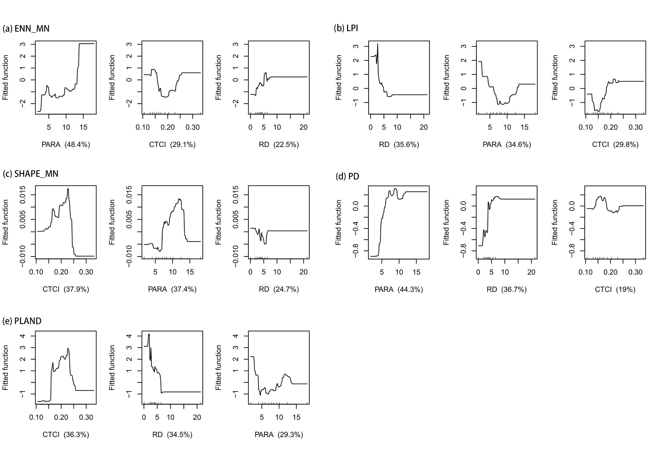
According to the results of BRT analysis (Figure 5), all three urban form metrics had important influences on the landscape metrics of UGS in China. The coefficient of variation (CV) for BRT model of ENN_MN, LPI, SHAPE_MN, PD, and PLAND were 0.205 (SE = 0.081), 0.211 (SE = 0.065), 0.349 (SE = 0.058), 0.26 (SE = 0.066), and 0.293 (SE = 0.049), respectively. The three urban form metrics can explain 23.2%, 31.6%, 31.1%, 23.3%, and 30.3% of deviance for ENN_MN, LPI, SHAPE_MN, PD, and PLAND, respectively. Among the three urban form metrics, PARA had the largest influence on ENN_MN (48.4%) and PD (44.3%). RD had strong influence on LPI (35.6%), PD (36.7%), and PLAND (34.5%). CTCI had the largest influence on SHAPE_MN (37.9%) and PLAND (36.3%). This indicated that different urban form metrics affect different dimensions of landscape structure.
4. Discussion
4.1. Landscape Structure of UGS in China
Our results revealed features of landscape structure of UGS in Chinese cities at the national scale. Dobbs et al. (2017) [23] investigated landscape structures of UGS for 100 cities worldwide and found that density of vegetation patch, nearest neighbor, and green cover of these cities were 0.33 count/ha (SD = 0.13 count/ha), 253.5 m (SD = 61.9 m), and 32.6% (SD = 12.1%), respectively. The percentage of UGS (i.e., PLAND) of Chinese cities was similar to world cities reported by Dobbs et al. (2017) [23]. However, UGS in Chinese cities were more fragmented (higher PD) and less isolated (lower ENN_MN). This agrees with a case study of nine major Chinese cities in which they found UGS of the nine cities were highly fragmented and heterogeneous [21]. This might be due to the fact that many Chinese cities have high population density (e.g., Hong Kong, Guangzhou, and Shanghai [53]), thus there are fewer spaces for large and homogeneous UGS to exist.
4.2. Impacts of Urban forms on Landscape Structure of UGS
We found that all three urban form metrics had significant effects on landscape structure of UGS. Cities with higher RD tended to have less UGS (lower PLAND value). This might because high RD is a feature of compact cities, which may have limited spaces for UGS [54]. Our results are in agreement with the study in Sheffield, UK [30] in which they found a negative relationship between extent of green space and total length of the roads network. We found that cities with higher RD tended to have more fragmented UGS (higher PD value). Urban landscape is often highly dissected by roads [55] and has fragmented UGS as a result.
Terrain complexity is a measure of terrain heterogeneity [49], which may positively affect the spatial distribution of UGS [30]. We found that CTCI affected landscape structure of UGS significantly. Cities with high terrain complexity tended to have more UGS (higher PLAND value), but UGS in these cities tended to be more fragmented (higher PD value). This observation was in agreement with the situation in Cincinnati, USA, in which the authors found that terrain roughness was positively correlated with the levels of tree canopy [31]. A study in 60 urban areas of Central Indiana, USA also found a positive relationship between urban tree canopy cover and slope of urban areas [56].
PARA indicates shape complexity of urban areas. We found that cities with complex shapes (higher PARA value) also had more fragmented UGS (higher PD value). In the USA, megapolitan areas with more complex shapes were found to have more complex and fragmented urban land covers than metropolitan areas with less complex shapes [57]. The same pattern was observed in Chinese cities through our study.
4.3. Implications for UGS Planning
Our study can provide some useful information for planning and management of UGS in China and other regions and countries facing rapid urbanization. Our results showed that urban form has a significant influence on landscape structure of UGS and must be considered in UGS planning. First, cities with high RD tended to have less and fragmented UGS. China is experiencing a rapid urbanization process and new roads are being built up consistently. When planning for new roads in Chinese cities, especially in cities with high RD, planners should pay attention to the existing UGS patches to avoid further fragmentation of UGS. Furthermore, to construct roadside greenway networks whenever possible may be a way to alleviate the negative effects associated with fragmentation caused by roads on UGS in cities with high RD. Roadside greenway networks have been found to act as important corridors for urban residents and wildlife [58]. In addition, innovative designs such as vegetated wildlife overpasses [59] and elevated linear parks [60] can be used to alleviate the fragmentation effects caused by roads. Besides, a vegetated drainage system can also be designed as a supplement to reverse habitat fragmentation and act as wildlife corridors and buffer zones [61].
Second, we found that cities with complex shapes often have more fragmented UGS. Urban planners should pay attention to the restriction caused by urban form when planning and designing the UGS system. Finally, our results showed that cities with high terrain complexities have more UGS but that these UGS are also more fragmented. There are both advantages and disadvantages when planning for UGS in cities with complex terrains. On the one hand, complex terrain may provide an opportunity to conserve green spaces in cities as it is difficult to develop on sites with complex terrain. On the other hand, planners must realize that corridors among green spaces are important for sustaining urban biodiversity [16] and should be preserved as much as possible. This task may be more difficult in cities with complex terrains because some sites are more isolated by the terrain. We call for actions to preserve natural pathways and corridors among green spaces in these cities during the development. The increased connectivity of green spaces can improve their ecological functions, such as their use as habitats by wildlife [62].
While our findings provide new knowledge on the influences of urban form on landscape structure of UGS, they should be interpreted with the limitations of the current study in mind. We only used a set of basic urban form and landscape metrics due to data availability. To use more metrics in future studies may reveal more details on the relationship between urban form and landscape structure of UGS. In addition, we only focused on cities with medium size and above where UGS are important due to their population sizes. The findings from our study may not be readily applicable to small cities. Despite these limitations, we showed that urban form has a significant influence on landscape structure of UGS using data retrieved from satellite images. The finding can contribute to better planning and management of UGS.
5. Conclusions
Landscape structure of UGS is closely related to urban ecosystem services [1,2]. Quantifying landscape structure of UGS and analyzing its influencing factors are important for managing ecosystem services for urban inhabitants’ health and wellbeing. We assessed the influences of urban form on landscape structure of UGS of 262 Chinese cities using Landsat images and the GEE platform. The GEE platform allowed us to obtain, preprocess, and classify 6673 scenes of Landsat images for 262 cities in a relatively short time. With the help of this geospatial analysis platform, we revealed the unique features of landscape structure of UGS in Chinese cities. We also showed that urban form had significant influences on landscape structure of UGS. Based on our results, we suggested that attention should be paid to urban form when planning and designing UGS. More urban form and landscape metrics can be considered in future studies to reveal more details of this relationship.
Supplementary Materials
The following are available online at https://www.mdpi.com/2072-4292/10/10/1569/s1, Table S1: Summary statistics of populations in 262 cities based on provinces, Table S2: Correlations between the five landscape metrics, Figure S1: Spatial distribution of Mean Euclidian nearest neighbor distance (ENN_MN, m) value, Figure S2: Spatial distribution of Largest Patch Index (LPI, %) value, Figure S3: Spatial distribution of Patch density (PD, count/km2) value, Figure S4: Spatial distribution of Mean patch shape index (SHAPE_MN) value, Supplementary file 1: Cities investigated in this study, and Supplementary file 2: Confusion matrix of land cover classification for each city.
Author Contributions
J.Y. designed the study and contributed to writing. C.H. conducted data analysis and wrote the paper. P.J. contributed to data analysis.
Funding
This study was supported by the National Natural Science Foundation of China (Grant number 31570458, 2016).
Acknowledgments
We want to thank Google for providing us free access to Google Earth Engine; we also thank Nicholas Clinton from Google for helping us with technical issues.
Conflicts of Interest
The authors declare no conflicts of interest.
References
- De la Barrera, F.; Reyes-Paecke, S.; Banzhaf, E. Indicators for green spaces in contrasting urban settings. Ecol. Indic. 2016, 62, 212–219. [Google Scholar] [CrossRef]
- Goddard, M.A.; Dougill, A.J.; Benton, T.G. Scaling up from gardens: Biodiversity conservation in urban environments. Trends Ecol. Evol. 2010, 25, 90–98. [Google Scholar] [CrossRef] [PubMed]
- United Nations. Sustainable Development Goals. Available online: http://www.Un.Org/sustainabledevelopment/sustainable-development-goals/ (accessed on 11 August 2018).
- Bolund, P.; Hunhammar, S. Ecosystem services in urban areas. Ecol. Econ. 1999, 29, 293–301. [Google Scholar] [CrossRef]
- Haase, D.; Larondelle, N.; Andersson, E.; Artmann, M.; Borgström, S.; Breuste, J.; Gomez-Baggethun, E.; Gren, Å.; Hamstead, Z.; Hansen, R. A quantitative review of urban ecosystem service assessments: Concepts, models, and implementation. Ambio 2014, 43, 413–433. [Google Scholar] [CrossRef] [PubMed]
- Akbari, H.; Cartalis, C.; Kolokotsa, D.; Muscio, A.; Pisello, A.L.; Rossi, F.; Santamouris, M.; Synnefa, A.; Wong, N.H.; Zinzi, M. Local climate change and urban heat island mitigation techniques–the state of the art. J. Civ. Eng. Manag. 2016, 22, 1–16. [Google Scholar] [CrossRef]
- Takács, Á.; Kiss, M.; Hof, A.; Tanács, E.; Gulyás, Á.; Kántor, N. Microclimate modification by urban shade trees–an integrated approach to aid ecosystem service based decision-making. Procedia Environ. Sci. 2016, 32, 97–109. [Google Scholar] [CrossRef]
- Zhang, Z.; Lv, Y.; Pan, H. Cooling and humidifying effect of plant communities in subtropical urban parks. Urban For. Urban Green. 2013, 12, 323–329. [Google Scholar] [CrossRef]
- Yang, J.; McBride, J.; Zhou, J.; Sun, Z. The urban forest in Beijing and its role in air pollution reduction. Urban For. Urban Green. 2005, 3, 65–78. [Google Scholar] [CrossRef]
- Zhang, B.; Li, N.; Wang, S. Effect of urban green space changes on the role of rainwater runoff reduction in Beijing, China. Landsc. Urban Plan. 2015, 140, 8–16. [Google Scholar] [CrossRef] [Green Version]
- White, M.P.; Alcock, I.; Wheeler, B.W.; Depledge, M.H. Would you be happier living in a greener urban area? A fixed-effects analysis of panel data. Psychol. Sci. 2013, 24, 920–928. [Google Scholar] [CrossRef] [PubMed]
- Maimaitiyiming, M.; Ghulam, A.; Tiyip, T.; Pla, F.; Latorre-Carmona, P.; Halik, Ü.; Sawut, M.; Caetano, M. Effects of green space spatial pattern on land surface temperature: Implications for sustainable urban planning and climate change adaptation. ISPRS J. Photogramm. Remote Sens. 2014, 89, 59–66. [Google Scholar] [CrossRef] [Green Version]
- Zhang, Y.; Murray, A.T.; Turner, B. Optimizing green space locations to reduce daytime and nighttime urban heat island effects in phoenix, arizona. Landsc. Urban Plan. 2017, 165, 162–171. [Google Scholar] [CrossRef]
- Mitchell, M.G.; Johansen, K.; Maron, M.; McAlpine, C.A.; Wu, D.; Rhodes, J.R. Identification of fine scale and landscape scale drivers of urban aboveground carbon stocks using high-resolution modeling and mapping. Sci. Total. Environ. 2018, 622, 57–70. [Google Scholar] [CrossRef] [PubMed]
- Xu, X.; Xie, Y.; Qi, K.; Luo, Z.; Wang, X. Detecting the response of bird communities and biodiversity to habitat loss and fragmentation due to urbanization. Sci. Total Environ. 2018, 624, 1561–1576. [Google Scholar] [CrossRef] [PubMed]
- Beninde, J.; Veith, M.; Hochkirch, A. Biodiversity in cities needs space: A meta-analysis of factors determining intra-urban biodiversity variation. Ecol. Lett. 2015, 18, 581–592. [Google Scholar] [CrossRef] [PubMed]
- Kong, F.; Nakagoshi, N. Spatial-temporal gradient analysis of urban green spaces in Jinan, China. Landsc. Urban Plan. 2006, 78, 147–164. [Google Scholar] [CrossRef]
- Gong, C.; Yu, S.; Joesting, H.; Chen, J. Determining socioeconomic drivers of urban forest fragmentation with historical remote sensing images. Landsc. Urban Plan. 2013, 117, 57–65. [Google Scholar] [CrossRef]
- Tian, Y.; Jim, C.; Tao, Y.; Shi, T. Landscape ecological assessment of green space fragmentation in Hong Kong. Urban For. Urban Green. 2011, 10, 79–86. [Google Scholar] [CrossRef]
- Uy, P.D.; Nakagoshi, N. Analyzing urban green space pattern and eco-network in Hanoi, Vietnam. Landsc. Ecol. Eng. 2007, 3, 143–157. [Google Scholar] [CrossRef]
- Zhou, W.; Wang, J.; Qian, Y.; Pickett, S.T.; Li, W.; Han, L. The rapid but “invisible” changes in urban greenspace: A comparative study of nine Chinese cities. Sci. Total Environ. 2018, 627, 1572–1584. [Google Scholar] [CrossRef]
- Richards, D.R.; Passy, P.; Oh, R.R. Impacts of population density and wealth on the quantity and structure of urban green space in tropical Southeast Asia. Landsc. Urban Plan. 2017, 157, 553–560. [Google Scholar] [CrossRef]
- Dobbs, C.; Nitschke, C.; Kendal, D. Assessing the drivers shaping global patterns of urban vegetation landscape structure. Sci. Total Environ. 2017, 592, 171–177. [Google Scholar] [CrossRef] [PubMed]
- Chen, B.; Nie, Z.; Chen, Z.; Xu, B. Quantitative estimation of 21st-century urban greenspace changes in Chinese populous cities. Sci. Total Environ. 2017, 609, 956–965. [Google Scholar] [CrossRef] [PubMed]
- Gorelick, N.; Hancher, M.; Dixon, M.; Ilyushchenko, S.; Thau, D.; Moore, R. Google earth engine: Planetary-scale geospatial analysis for everyone. Remote Sens. Environ. 2017, 202, 18–27. [Google Scholar] [CrossRef]
- Goldblatt, R.; You, W.; Hanson, G.; Khandelwal, A.K. Detecting the boundaries of urban areas in India: A dataset for pixel-based image classification in google earth engine. Remote Sens. 2016, 8, 634. [Google Scholar] [CrossRef]
- Trianni, G.; Lisini, G.; Angiuli, E.; Moreno, E.; Dondi, P.; Gaggia, A.; Gamba, P. Scaling up to national/regional urban extent mapping using landsat data. IEEE J. Sel. Top. Appl. Earth Obs. Remote Sens. 2015, 8, 3710–3719. [Google Scholar] [CrossRef]
- Huang, C.; Yang, J.; Lu, H.; Huang, H.; Yu, L. Green spaces as an indicator of urban health: Evaluating its changes in 28 mega-cities. Remote Sens. 2017, 9, 1266. [Google Scholar] [CrossRef]
- Anderson, W.P.; Kanaroglou, P.S.; Miller, E.J. Urban form, energy and the environment: A review of issues, evidence and policy. Urban Stud. 1996, 33, 7–35. [Google Scholar] [CrossRef]
- Davies, R.G.; Barbosa, O.; Fuller, R.A.; Tratalos, J.; Burke, N.; Lewis, D.; Warren, P.H.; Gaston, K.J. City-wide relationships between green spaces, urban land use and topography. Urban Ecosyst. 2008, 11, 269. [Google Scholar] [CrossRef]
- Berland, A.; Schwarz, K.; Herrmann, D.L.; Hopton, M.E. How environmental justice patterns are shaped by place: Terrain and tree canopy in Cincinnati, Ohio, USA. Cities Environ. 2015, 8, 1. [Google Scholar]
- United Nations. World Urbanization Prospects: The 2014 Revision; Department of Economic and Social Affairs: New York, NY, USA, 2014. [Google Scholar]
- Foga, S.; Scaramuzza, P.L.; Guo, S.; Zhu, Z.; Dilley, R.D.; Beckmann, T.; Schmidt, G.L.; Dwyer, J.L.; Hughes, M.J.; Laue, B. Cloud detection algorithm comparison and validation for operational landsat data products. Remote Sens. Environ. 2017, 194, 379–390. [Google Scholar] [CrossRef]
- Zhu, Z.; Wang, S.; Woodcock, C.E. Improvement and expansion of the fmask algorithm: Cloud, cloud shadow, and snow detection for landsats 4–7, 8, and sentinel 2 images. Remote Sens. Environ. 2015, 159, 269–277. [Google Scholar] [CrossRef]
- Zhu, Z.; Woodcock, C.E. Object-based cloud and cloud shadow detection in landsat imagery. Remote Sens. Environ. 2012, 118, 83–94. [Google Scholar] [CrossRef]
- Tucker, C.J. Red and photographic infrared linear combinations for monitoring vegetation. Remote Sens. Environ. 1979, 8, 127–150. [Google Scholar] [CrossRef] [Green Version]
- Zha, Y.; Gao, J.; Ni, S. Use of normalized difference built-up index in automatically mapping urban areas from tm imagery. Int. J. Remote Sens. 2003, 24, 583–594. [Google Scholar] [CrossRef]
- Xu, H. Modification of normalised difference water index (NDWI) to enhance open water features in remotely sensed imagery. Int. J. Remote Sens. 2006, 27, 3025–3033. [Google Scholar] [CrossRef]
- Hansen, M.C.; Potapov, P.V.; Moore, R.; Hancher, M.; Turubanova, S.; Tyukavina, A.; Thau, D.; Stehman, S.; Goetz, S.; Loveland, T. High-resolution global maps of 21st-century forest cover change. Science 2013, 342, 850–853. [Google Scholar] [CrossRef] [PubMed]
- Azzari, G.; Lobell, D. Landsat-based classification in the cloud: An opportunity for a paradigm shift in land cover monitoring. Remote Sens. Environ. 2017, 202, 64–74. [Google Scholar] [CrossRef]
- Schneider, A.; Friedl, M.A.; Potere, D. Mapping global urban areas using modis 500-m data: New methods and datasets based on ‘urban ecoregions’. Remote Sens. Environ. 2010, 114, 1733–1746. [Google Scholar] [CrossRef]
- Breiman, L. Random forests. Mach. Learn. 2001, 45, 5–32. [Google Scholar] [CrossRef]
- Olofsson, P.; Foody, G.M.; Herold, M.; Stehman, S.V.; Woodcock, C.E.; Wulder, M.A. Good practices for estimating area and assessing accuracy of land change. Remote Sens. Environ. 2014, 148, 42–57. [Google Scholar] [CrossRef] [Green Version]
- Zhou, Y.; Smith, S.J.; Zhao, K.; Imhoff, M.; Thomson, A.; Bond-Lamberty, B.; Asrar, G.R.; Zhang, X.; He, C.; Elvidge, C.D. A global map of urban extent from nightlights. Environ. Res. Lett. 2015, 10, 054011. [Google Scholar] [CrossRef] [Green Version]
- Grafius, D.R.; Corstanje, R.; Harris, J.A. Linking ecosystem services, urban form and green space configuration using multivariate landscape metric analysis. Landsc. Ecol. 2018, 33, 557–573. [Google Scholar] [CrossRef] [Green Version]
- Li, X.; Zhou, W.; Ouyang, Z.; Xu, W.; Zheng, H. Spatial pattern of greenspace affects land surface temperature: Evidence from the heavily urbanized Beijing metropolitan area, China. Landsc. Ecol. 2012, 27, 887–898. [Google Scholar] [CrossRef]
- McGarigal, K. Fragstats Help; University of Massachusetts: Amherst, MA, USA, 2015. [Google Scholar]
- Lu, H.; Liu, X.; Bian, L. Terrain Complexity: Definition, Index, and DEM Resolution. Proc. SPIE 2007, 6753, 675323. [Google Scholar]
- Yu, F.; Wang, T.; Groen, T.A.; Skidmore, A.K.; Yang, X.; Geng, Y.; Ma, K. Multi-scale comparison of topographic complexity indices in relation to plant species richness. Ecol. Complex. 2015, 22, 93–101. [Google Scholar] [CrossRef]
- Ou, J.; Liu, X.; Li, X.; Chen, Y. Quantifying the relationship between urban forms and carbon emissions using panel data analysis. Landsc. Ecol. 2013, 28, 1889–1907. [Google Scholar] [CrossRef]
- Farr, T.G.; Rosen, P.A.; Caro, E.; Crippen, R.; Duren, R.; Hensley, S.; Kobrick, M.; Paller, M.; Rodriguez, E.; Roth, L. The shuttle radar topography mission. Rev. Geophys. 2007, 45. [Google Scholar] [CrossRef]
- Reshef, D.N.; Reshef, Y.A.; Finucane, H.K.; Grossman, S.R.; McVean, G.; Turnbaugh, P.J.; Lander, E.S.; Mitzenmacher, M.; Sabeti, P.C. Detecting novel associations in large data sets. Science 2011, 334, 1518–1524. [Google Scholar] [CrossRef] [PubMed]
- Bertaud, A. The Spatial Organization of Cities: Deliberate Outcome or Unforeseen Consequence? Available online: https://escholarship.org/uc/item/5vb4w9wb (accessed on 29 September 2018).
- Jim, C.Y. Green-space preservation and allocation for sustainable greening of compact cities. Cities 2004, 21, 311–320. [Google Scholar] [CrossRef]
- Weng, Y.-C. Spatiotemporal changes of landscape pattern in response to urbanization. Landsc. Urban Plan. 2007, 81, 341–353. [Google Scholar] [CrossRef]
- Heynen, N.C.; Lindsey, G. Correlates of urban forest canopy cover: Implications for local public works. Public Works Manag. Policy 2003, 8, 33–47. [Google Scholar] [CrossRef]
- Bereitschaft, B.; Debbage, K. Regional variations in urban fragmentation among us metropolitan and megapolitan areas. Appl. Spat. Anal. Policy 2014, 7, 119–147. [Google Scholar] [CrossRef]
- Li, F.; Wang, R.; Paulussen, J.; Liu, X. Comprehensive concept planning of urban greening based on ecological principles: A case study in Beijing, China. Landsc. Urban Plan. 2005, 72, 325–336. [Google Scholar] [CrossRef]
- Corlatti, L.; Hacklaender, K.; Frey-Roos, F. Ability of wildlife overpasses to provide connectivity and prevent genetic isolation. Conserv. Boil. 2009, 23, 548–556. [Google Scholar] [CrossRef] [PubMed]
- Sinha, A. Slow landscapes of elevated linear parks: Bloomingdale trail in Chicago. Stud. Hist. Gard. Des. Landsc. 2014, 34, 113–122. [Google Scholar] [CrossRef]
- Mak, C.; Scholz, M.; James, P. Sustainable drainage system site assessment method using urban ecosystem services. Urban Ecosyst. 2017, 20, 293–307. [Google Scholar] [CrossRef]
- Jim, C.Y.; Chen, S.S. Comprehensive greenspace planning based on landscape ecology principles in compact Nanjing City, China. Landsc. Urban Plan. 2003, 65, 95–116. [Google Scholar] [CrossRef]
Figure 1.
Locations of the 262 studied Chinese cities.

Figure 2.
Summary statistics of landscape metrics of urban green spaces, (a) percentage of landscape, (b) patch density, (c) largest patch index, (d) mean patch shape index, and (e) mean Euclidian nearest neighbor distance. The box shows median, 25th and 75th percentile, and the whiskers illustrate the 5th and 95th percentile values.

Figure 3.
PLAND (percentage of landscape, %) values of UGS in 262 cities.

Figure 4.
Examples of the distribution of urban green spaces and their landscape structures for cities with: (a) low compound terrain complexity index value (Zaozhuang, Shandong), (b) high compound terrain complexity index value (Chengde, Hebei), (c) low perimeter-area ratio value (Wuxi, Jiangsu), (d) high perimeter-area ratio value (Haimen, Jiangsu), (e) low road density (Shaoguan, Guangdong), and (f) high road density value (Changchun, Jilin). CTCI, compound terrain complexity index; PARA, perimeter-area ratio; RD, road density.

Figure 5.
Partial dependence plots for boosted regression tree analysis showing the effects of urban form predictors on: (a) ENN_MN (mean Euclidian nearest neighbor distance), (b) LPI (largest patch index), (c) SHAPE_MN (mean patch shape index), (d) PD (patch density), and (e) PLAND (percentage of landscape). Numbers enclosed inside parenthesis indicated the relative importance of predictors. CTCI, compound terrain complexity index; PARA, perimeter-area ratio; RD, road density.


Table 1.
Descriptions of the landscape metrics [47].
Table 1.
Descriptions of the landscape metrics [47].
| Landscape Metrics | Description | Unit | Range |
|---|---|---|---|
| Mean Euclidian nearest neighbor distance (ENN_MN) | ENN_MN refers to mean distance to the nearest neighboring patch of urban green spaces based on the edge-to-edge distance | m | ENN_MN > 0 |
| Largest Patch Index (LPI) | LPI equals the area (m2) of the largest patch of the corresponding patch type divided by total landscape area (m2), multiplied by 100 (to convert to a percentage). | % | 0 < LPI ≤ 100 |
| Mean patch shape index (SHAPE_MN) | SHAPE_MN refers to the mean value of patch shape index | None | SHAPE_MN ≥ 1 |
| Patch density (PD) | PD equals the number of patches in the landscape, divided by total landscape area (m2), multiplied by 10,000 and 100 (to covert to 100 hectares). | count/km2 | PD > 0 |
| Percentage of landscape (PLAND) | PLAND equals the area of urban green spaces divided by the area of built-up area. | % | 0 < PLAND ≤ 100 |
Table 2.
Associations between landscape metrics and the urban form metrics.
| Factors | CTCI | PARA | RD | ||||||
|---|---|---|---|---|---|---|---|---|---|
| MIC | MIC-ρ2 | ρ | MIC | MIC-ρ2 | ρ | MIC | MIC-ρ2 | ρ | |
| ENN_MN | 0.19 | 0.19 | −0.02 | 0.26 ** | 0.23 | 0.16 * | 0.20 | 0.19 | 0.12 * |
| LPI | 0.21 | 0.20 | 0.13 * | 0.22 | 0.22 | 0.002 | 0.25 * | 0.23 | −0.14 * |
| SHAPE_MN | 0.26 ** | 0.26 | 0.07 | 0.26 ** | 0.24 | 0.13 * | 0.21 | 0.21 | −0.02 |
| PD | 0.24 * | 0.23 | 0.10 | 0.23 | 0.18 | 0.23 *** | 0.23 | 0.23 | 0.05 |
| PLAND | 0.22 | 0.20 | 0.15 * | 0.21 | 0.21 | 0.03 | 0.20 | 0.18 | −0.14 * |
MIC, maximal information coefficient; MIC-ρ2, nonlinearity coefficient; ρ, Pearson correlation coefficient. CTCI, compound terrain complexity index; PARA, perimeter-area ratio; RD, road density; ENN_MN, mean Euclidian nearest neighbor distance; LPI, largest patch index; SHAPE_MN, mean patch shape index; PD, patch density; PLAND, percentage of landscape. *** p < 0.001. ** p < 0.01. * p < 0.05.
© 2018 by the authors. Licensee MDPI, Basel, Switzerland. This article is an open access article distributed under the terms and conditions of the Creative Commons Attribution (CC BY) license (http://creativecommons.org/licenses/by/4.0/).
Share and Cite
MDPI and ACS Style
Huang, C.; Yang, J.; Jiang, P. Assessing Impacts of Urban Form on Landscape Structure of Urban Green Spaces in China Using Landsat Images Based on Google Earth Engine. Remote Sens. 2018, 10, 1569. https://doi.org/10.3390/rs10101569
AMA Style
Huang C, Yang J, Jiang P. Assessing Impacts of Urban Form on Landscape Structure of Urban Green Spaces in China Using Landsat Images Based on Google Earth Engine. Remote Sensing. 2018; 10(10):1569. https://doi.org/10.3390/rs10101569
Chicago/Turabian StyleHuang, Conghong, Jun Yang, and Peng Jiang. 2018. "Assessing Impacts of Urban Form on Landscape Structure of Urban Green Spaces in China Using Landsat Images Based on Google Earth Engine" Remote Sensing 10, no. 10: 1569. https://doi.org/10.3390/rs10101569
Note that from the first issue of 2016, this journal uses article numbers instead of page numbers. See further details here.