Multifrequency and Full-Polarimetric SAR Assessment for Estimating Above Ground Biomass and Leaf Area Index in the Amazon Várzea Wetlands

 ,
,  and
and 
Abstract
:
1. Introduction
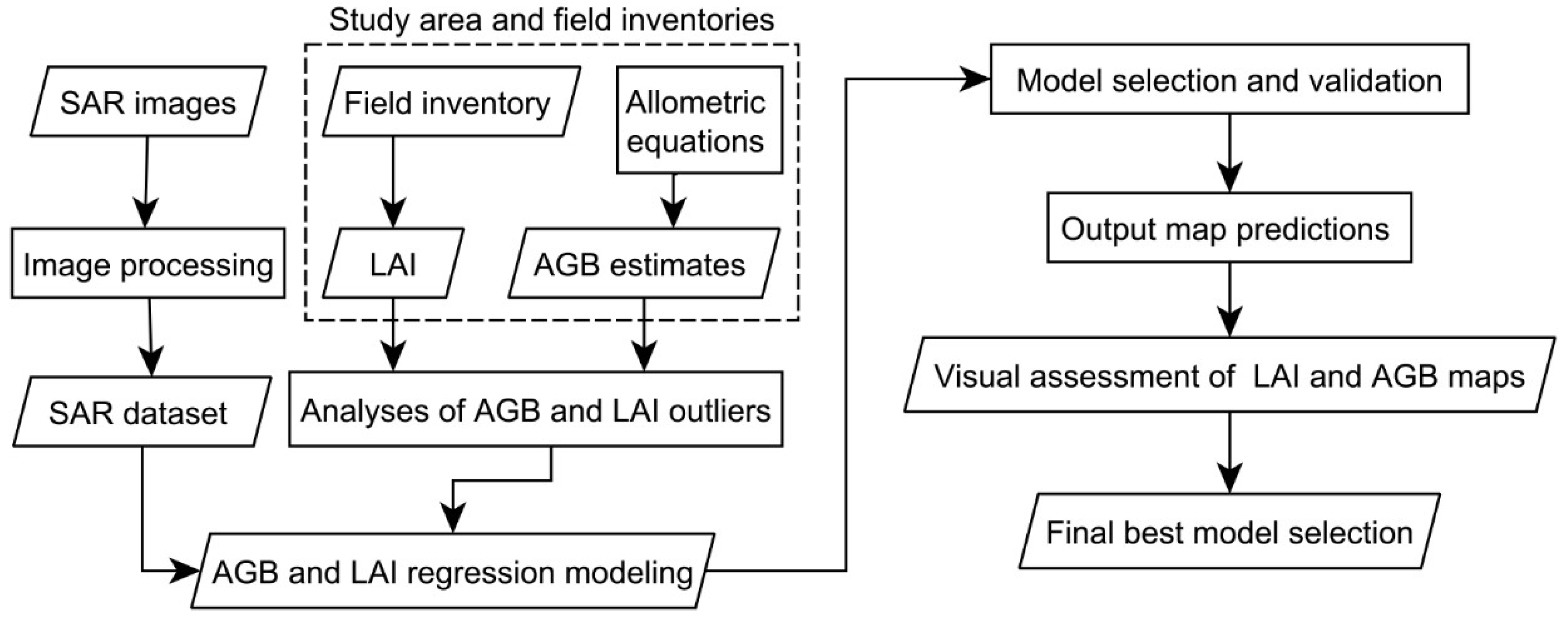
2. Materials and Methods
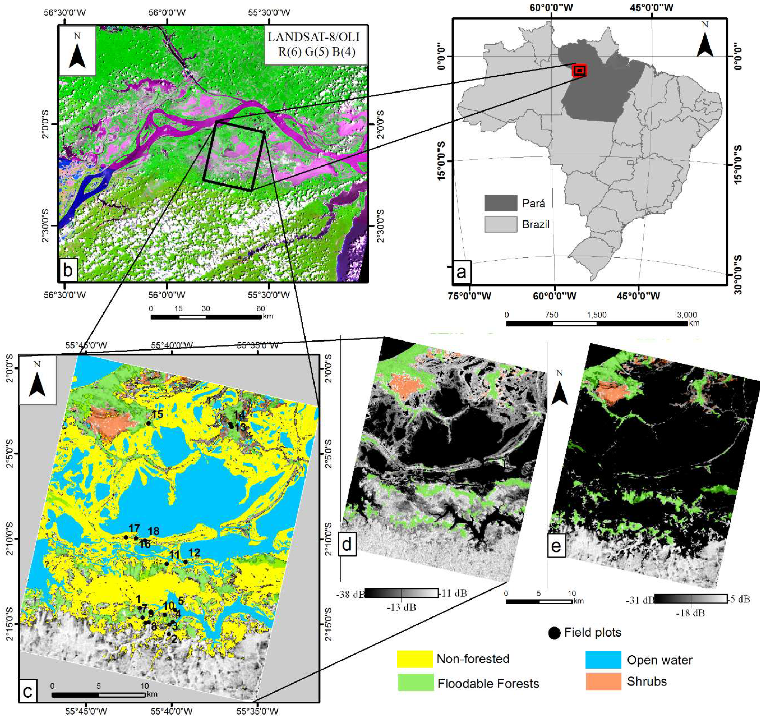
2.1. Study Area and Field Inventories
2.2. SAR Image Acquisition
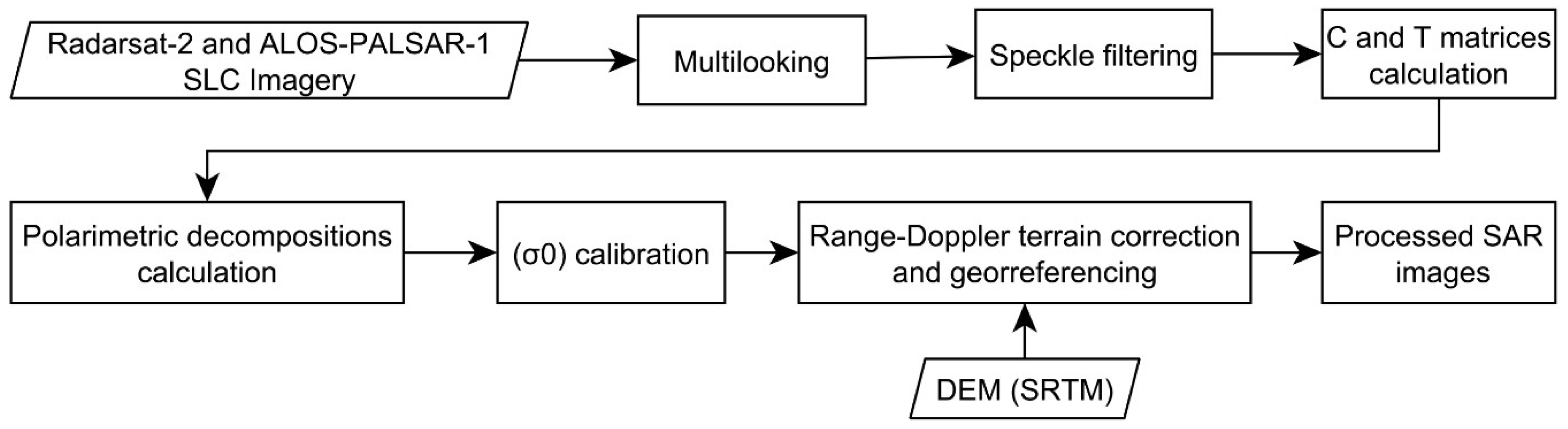
2.3. Image Processing
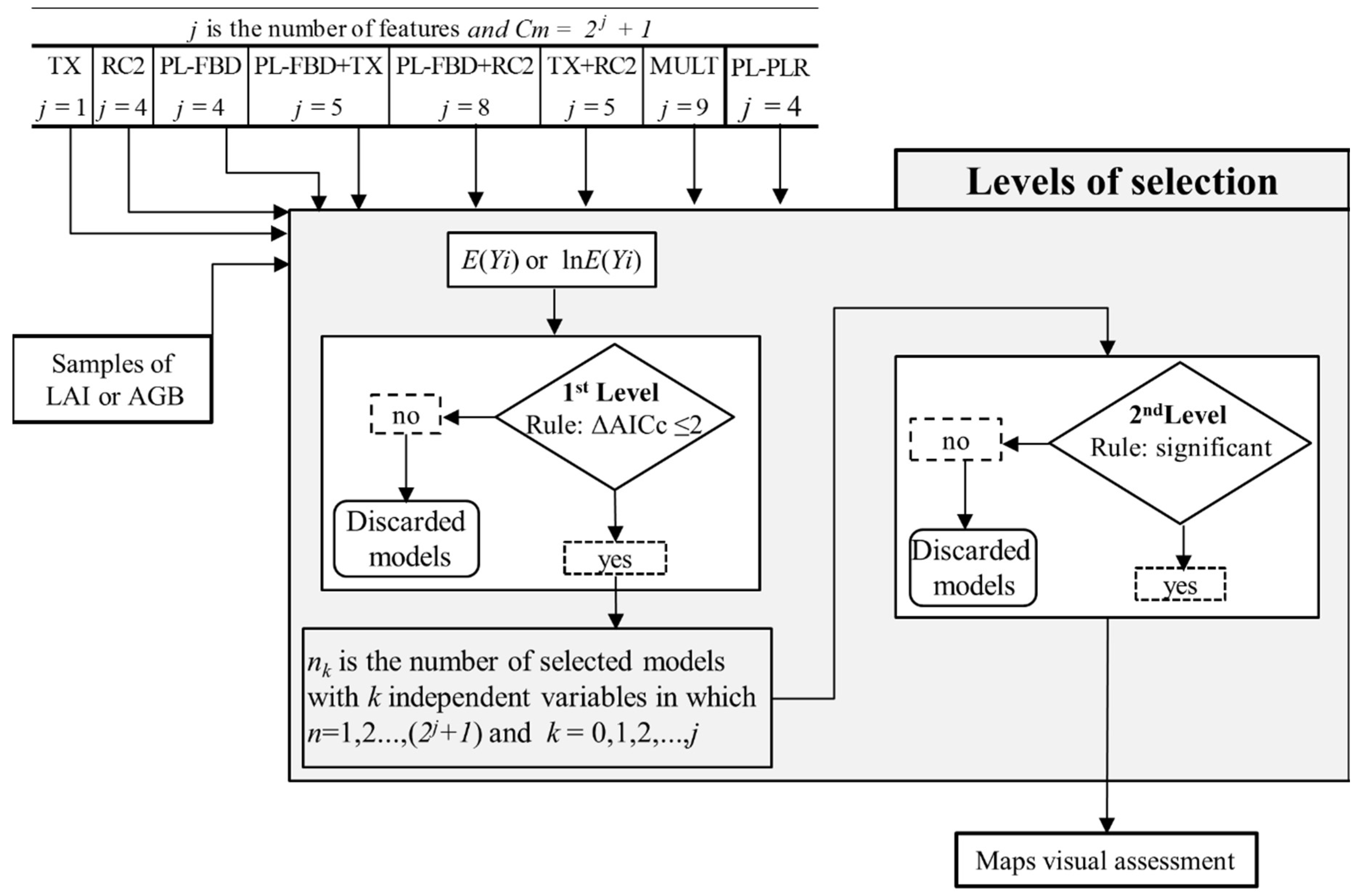
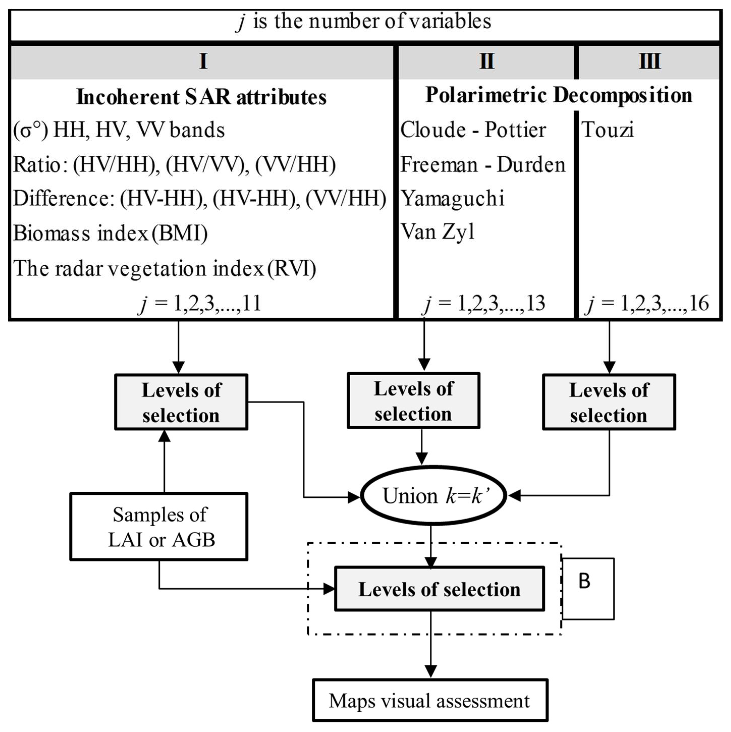
2.4. Assembly of SAR Modeling Sets
2.5. Above Ground Biomass and Leaf Area Index Modeling
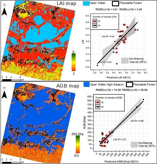
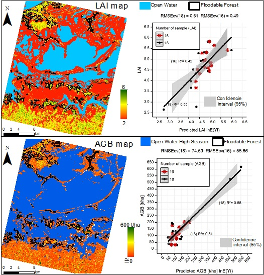
2.6. Visual Assessment of Maps LAI and AGB Maps
3. Results
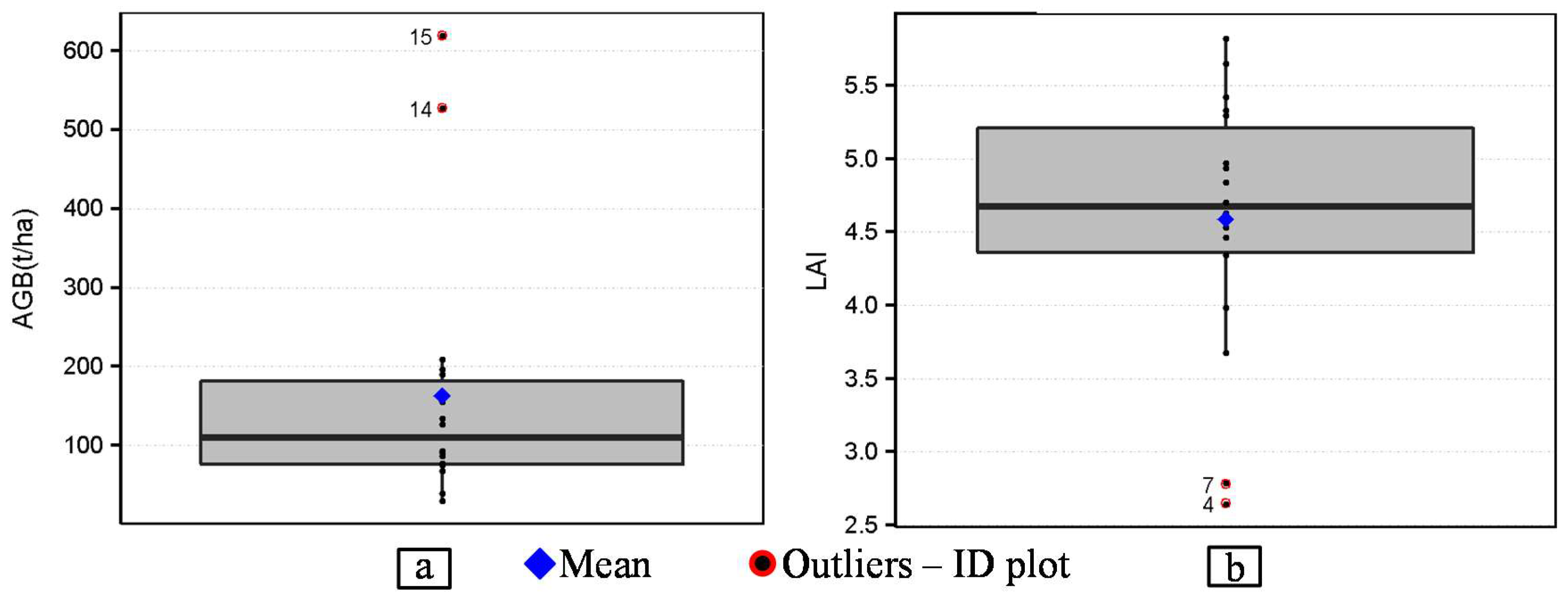
3.1. Exploratory Analysis of LAI and AGB Data
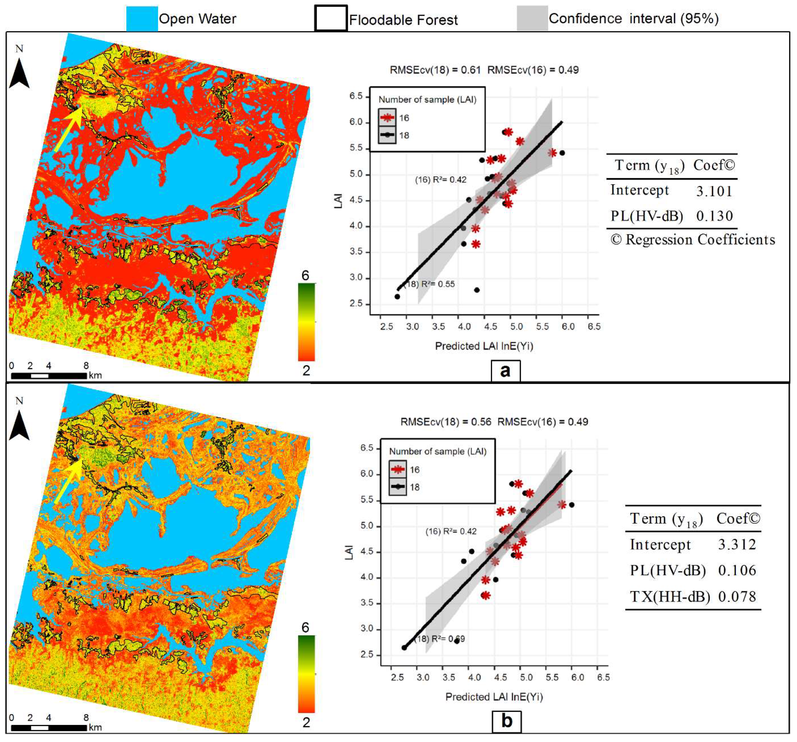
3.2. LAI Models
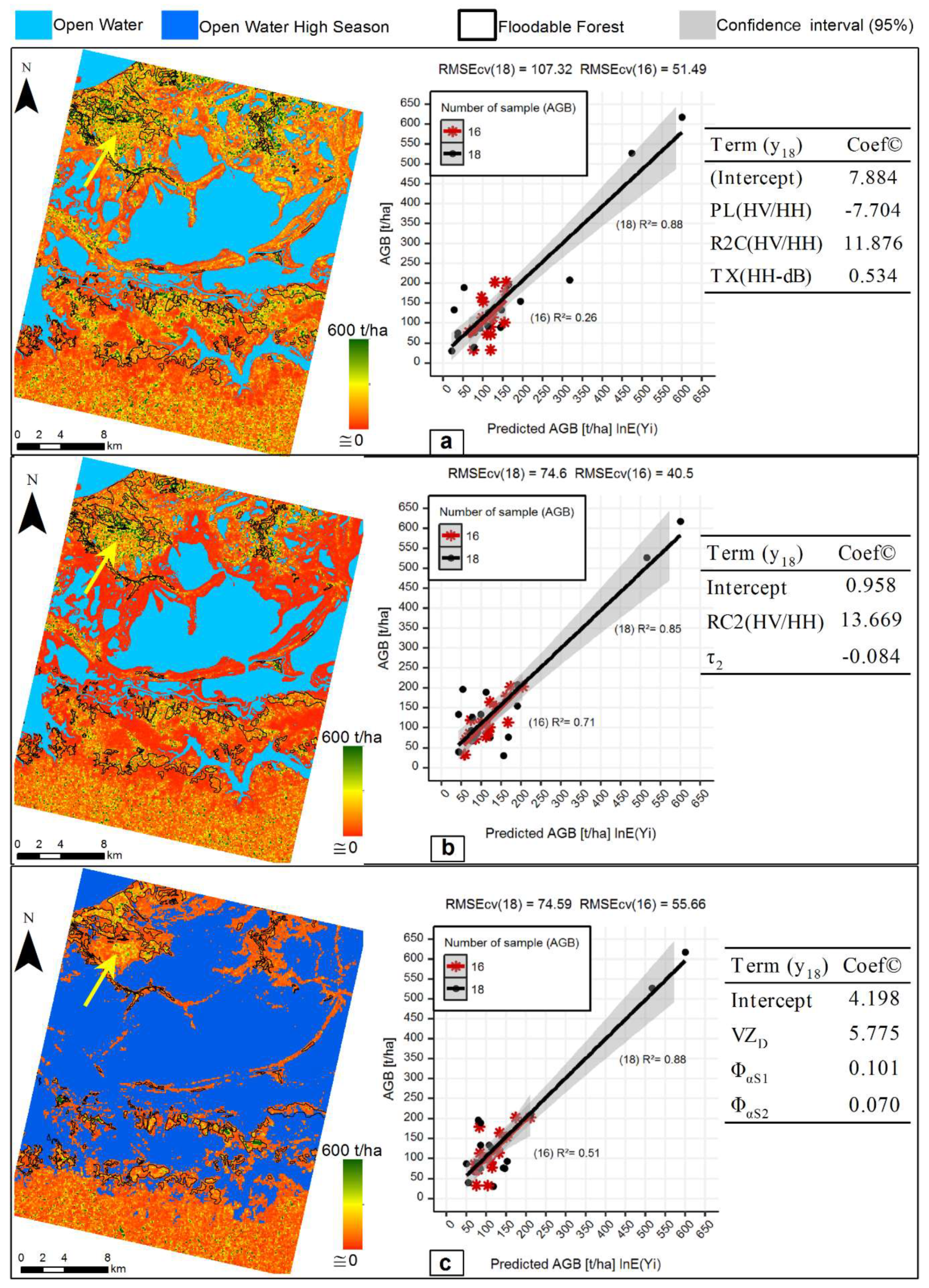
3.3. AGB Regression Models
4. Discussion
5. Conclusions
Supplementary Materials
Author Contributions
Funding
Acknowledgments
Conflicts of Interest
References
- Gibbs, H.K.; Brown, S.; Niles, J.O.; Foley, J.A. Monitoring and estimating tropical forest carbon stocks: Making redd a reality. Environ. Res. Lett. 2007, 2, 45023. [Google Scholar] [CrossRef]
- Asner, G.P. Cloud cover in Landsat observations of the brazilian Amazon. Int. J. Remote Sens. 2010, 22, 3855–3862. [Google Scholar] [CrossRef]
- Kumar, L.; Sinha, P.; Taylor, S.; Alqurashi, A.F. Review of the Use of Remote Sensing for Biomass Estimation to Support Renewable Energy Generation; SPIE: Bellingham, WA, USA, 2015; p. 28. [Google Scholar]
- Lu, D. The potential and challenge of remote sensing-based biomass estimation. Int. J. Remote Sens. 2006, 27, 1297–1328. [Google Scholar] [CrossRef]
- Lu, D.; Chen, Q.; Wang, G.; Liu, L.; Li, G.; Moran, E. A survey of remote sensing-based aboveground biomass estimation methods in forest ecosystems. Int. J. Digit. Earth 2014, 9, 63–105. [Google Scholar] [CrossRef]
- Henderson, F.M.; Lewis, A.J. Radar detection of wetland ecosystems: A review. Int. J. Remote Sens. 2008, 29, 5809–5835. [Google Scholar] [CrossRef]
- Silva, T.; Melack, J.; Streher, A.; Ferreira-Ferreira, J.; de Almeida Furtado, L. Capturing the dynamics of amazonian wetlands using synthetic aperture radar: Lessons learned and future directions. In Remote Sensing of Wetlands: Applications and Advances; CRC Press: Boca Raton, FL, USA, 2015; pp. 453–470. [Google Scholar]
- Furtado, L.F.A.; Silva, T.S.F.; Novo, E.M.L.M. Dual-season and full-polarimetric C band SAR assessment for vegetation mapping in the Amazon várzea wetlands. Remote Sens. Environ. 2016, 174, 212–222. [Google Scholar] [CrossRef]
- Hess, L.L.; Melack, J.M.; Simonett, D.S. Radar detection of flooding beneath the forest canopy: A review. Int. J. Remote Sens. 1990, 11, 1313–1325. [Google Scholar] [CrossRef]
- Silva, T.S.F.; Costa, M.P.F.; Melack, J.M. Spatial and temporal variability of macrophyte cover and productivity in the eastern Amazon floodplain: A remote sensing approach. Remote Sens. Environ. 2010, 114, 1998–2010. [Google Scholar] [CrossRef]
- Lee, J.S.; Pottier, E. Polarimetric Radar Imaging: From Basics to Applications; CRC Press: Boca Raton, FL, USA, 2009. [Google Scholar]
- Sartori, L.R.; Imai, N.N.; Mura, J.C.; Novo, E.M.L.d.M.; Silva, T.S.F. Mapping macrophyte species in the Amazon floodplain wetlands using fully polarimetric ALOS/PALSAR data. IEEE Trans. Geosci. Remote Sens. 2011, 49, 4717–4728. [Google Scholar] [CrossRef]
- Ranson, K.J.; Saatchi, S.; Guoqing, S. Boreal forest ecosystem characterization with SIR-C/XSAR. IEEE Trans. Geosci. Remote Sens. 1995, 33, 867–876. [Google Scholar] [CrossRef]
- Ranson, K.J.; Sun, G. An evaluation of AIRSAR and SIR-C/X-SAR images for mapping northern forest attributes in maine, USA. Remote Sens. Environ. 1997, 59, 203–222. [Google Scholar] [CrossRef]
- Novo, E.M.L.M.; Costa, M.P.F.; Jose, E.M.; Lima, I.B.T. Relationship between macrophyte stand variables and radar backscatter at L and C band, Tucuruí reservoir, Brazil. Int. J. Remote Sens. 2002, 23, 1241–1260. [Google Scholar] [CrossRef]
- Proisy, C.; Mougin, E.; Fromard, F.; Trichon, V.; Karam, M.A. On the influence of canopy structure on the radar backscattering of mangrove forests. Int. J. Remote Sens. 2002, 23, 4197–4210. [Google Scholar] [CrossRef]
- Saatchi, S.; Halligan, K.; Despain, D.G.; Crabtree, R.L. Estimation of forest fuel load from radar remote sensing. IEEE Trans. Geosci. Remote Sens. 2007, 45, 1726–1740. [Google Scholar] [CrossRef]
- Kovacs, J.M.; Jiao, X.; Flores-de-Santiago, F.; Zhang, C.; Flores-Verdugo, F. Assessing relationships between Radarsat-2 C-band and structural parameters of a degraded mangrove forest. Int. J. Remote Sens. 2013, 34, 7002–7019. [Google Scholar] [CrossRef]
- Huang, W.; Sun, G.; Ni, W.; Zhang, Z.; Dubayah, R. Sensitivity of multi-source SAR backscatter to changes in forest aboveground biomass. Remote Sens. 2015, 7, 9587–9609. [Google Scholar] [CrossRef]
- Sinha, S.; Jeganathan, C.; Sharma, L.K.; Nathawat, M.S. A review of radar remote sensing for biomass estimation. Int. J. Environ. Sci. Technol. 2015, 12, 1779–1792. [Google Scholar] [CrossRef] [Green Version]
- Costa, M.P.F.; Niemann, O.; Novo, E.; Ahern, F. Biophysical properties and mapping of aquatic vegetation during the hydrological cycle of the Amazon floodplain using JERS-1 and Radarsat. Int. J. Remote Sens. 2002, 23, 1401–1426. [Google Scholar] [CrossRef]
- Costa, M.P.F. Use of SAR satellites for mapping zonation of vegetation communities in the Amazon floodplain. Int. J. Remote Sens. 2004, 25, 1817–1835. [Google Scholar] [CrossRef]
- Hess, L.L.; Melack, J.M.; Davis, F.W. Mapping of floodplain inundation with multi-frequency polarimetric SAR: Use of a tree-based model. In Proceedings of the IGARSS ‘94—1994 IEEE International Geoscience and Remote Sensing Symposium, Pasadena, CA, USA, 8–12 August 1994; pp. 1072–1073. [Google Scholar]
- Pandey, U.; Kushwaha, S.; Kachhwaha, T.; Kunwar, P.; Dadhwal, V. Potential of Envisat ASAR data for woody biomass assessment. Trop. Ecol. 2010, 51, 117. [Google Scholar]
- Treuhaft, R.; Lei, Y.; Gonçalves, F.; Keller, M.; dos Santos, J.R.; Neumann, M.; Almeida, A. Tropical-forest structure and biomass dynamics from TanDEM-X radar interferometry. Forests 2017, 8, 277. [Google Scholar] [CrossRef]
- Luckman, A.; Baker, J.; Kuplich, T.M.; Corina da Costa, F.Y.; Alejandro, C.F. A study of the relationship between radar backscatter and regenerating tropical forest biomass for spaceborne SAR instruments. Remote Sens. Environ. 1997, 60, 1–13. [Google Scholar] [CrossRef]
- Kuplich, T.M.; Curran, P.J.; Atkinson, P.M. Relating SAR image texture to the biomass of regenerating tropical forests. Int. J. Remote Sens. 2005, 26, 4829–4854. [Google Scholar] [CrossRef]
- Kuplich, T.M.; Salvatori, V.; Curran, P.J. JERS-1/SAR backscatter and its relationship with biomass of regenerating forests. Int. J. Remote Sens. 2000, 21, 2513–2518. [Google Scholar] [CrossRef]
- Santos, J.R.; Pardi Lacruz, M.S.; Araujo, L.S.; Keil, M. Savanna and tropical rainforest biomass estimation and spatialization using JERS-1 data. Int. J. Remote Sens. 2002, 23, 1217–1229. [Google Scholar] [CrossRef]
- Austin, J.M.; Mackey, B.G.; Van Niel, K.P. Estimating forest biomass using satellite radar: An exploratory study in a temperate australian eucalyptus forest. For. Ecol. Manag. 2003, 176, 575–583. [Google Scholar] [CrossRef]
- Morel, A.C.; Saatchi, S.S.; Malhi, Y.; Berry, N.J.; Banin, L.; Burslem, D.; Nilus, R.; Ong, R.C. Estimating aboveground biomass in forest and oil palm plantation in sabah, Malaysian borneo using ALOS PALSAR data. For. Ecol. Manag. 2011, 262, 1786–1798. [Google Scholar] [CrossRef]
- Englhart, S.; Keuck, V.; Siegert, F. Aboveground biomass retrieval in tropical forests—The potential of combined X- and L-band SAR data use. Remote Sens. Environ. 2011, 115, 1260–1271. [Google Scholar] [CrossRef]
- Carreiras, J.M.B.; Jones, J.; Lucas, R.M.; Shimabukuro, Y.E. Mapping major land cover types and retrieving the age of secondary forests in the brazilian Amazon by combining single-date optical and radar remote sensing data. Remote Sens. Environ. 2017, 194, 16–32. [Google Scholar] [CrossRef]
- Berninger, A.; Lohberger, S.; Stängel, M.; Siegert, F. SAR-based estimation of above-ground biomass and its changes in tropical forests of Kalimantan using L- and C-Band. Remote Sens. 2018, 10, 831. [Google Scholar] [CrossRef]
- Lucas, R.; Bunting, P.; Clewley, D.; Armston, J.; Fairfax, R.; Fensham, R.; Accad, A.; Kelley, J.; Laidlaw, M.; Eyre, T.; et al. An evaluation of the ALOS PALSAR L-Band backscatter—Above ground biomass relationship queensland, Australia: Impacts of surface moisture condition and vegetation structure. IEEE J. Sel. Top. Appl. Earth Obs. Remote Sens. 2010, 3, 576–593. [Google Scholar] [CrossRef]
- Mitchard, E.T.A.; Saatchi, S.S.; Woodhouse, I.H.; Nangendo, G.; Ribeiro, N.S.; Williams, M.; Ryan, C.M.; Lewis, S.L.; Feldpausch, T.R.; Meir, P. Using satellite radar backscatter to predict above-ground woody biomass: A consistent relationship across four different African landscapes. Geophys. Res. Lett. 2009, 36. [Google Scholar] [CrossRef] [Green Version]
- Wittmann, F.; Schöngart, J.; Junk, W.J. Phytogeography, species diversity, community structure and dynamics of central amazonian floodplain forests. In Amazonian Floodplain Forests; Springer: Berlin, Germany, 2010; pp. 61–102. [Google Scholar]
- Arraut, E.M.; Marmontel, M.; Mantovani, J.E.; Novo, E.M.L.M.; Macdonald, D.W.; Kenward, R.E. The lesser of two evils: Seasonal migrations of amazonian manatees in the western Amazon. J. Zool. 2010, 280, 247–256. [Google Scholar] [CrossRef]
- Arantes, C.C.; Castello, L.; Cetra, M.; Schilling, A. Environmental influences on the distribution of arapaima in Amazon floodplains. Environ. Boil. Fishes 2013, 96, 1257–1267. [Google Scholar] [CrossRef]
- Melack, J.M.; Hess, L.L. Remote sensing of the distribution and extent of wetlands in the Amazon basin. In Amazonian Floodplain Forests; Springer: Berlin, Germany, 2010; pp. 43–59. [Google Scholar]
- Hawes, J.E.; Peres, C.A.; Riley, L.B.; Hess, L.L. Landscape-scale variation in structure and biomass of amazonian seasonally flooded and unflooded forests. For. Ecol. Manag. 2012, 281, 163–176. [Google Scholar] [CrossRef]
- Castello, L.; McGrath, D.G.; Hess, L.L.; Coe, M.T.; Lefebvre, P.A.; Petry, P.; Macedo, M.N.; Renó, V.F.; Arantes, C.C. The vulnerability of Amazon freshwater ecosystems. Conserv. Lett. 2013, 6, 217–229. [Google Scholar] [CrossRef] [Green Version]
- Renó, V.; Novo, E.; Suemitsu, C.; Rennó, C.; Silva, T. Assessment of deforestation in the lower Amazon floodplain using historical Landsat MSS/TM imagery. Remote Sens. Environ. 2011, 115, 3446–3456. [Google Scholar] [CrossRef]
- Fragal, E.H.; Silva, T.S.F.; Novo, E.M.L.D.M. Reconstructing historical forest cover change in the lower Amazon floodplains using the landtrendr algorithm. Acta Amaz. 2016, 46, 13–24. [Google Scholar] [CrossRef]
- Inoue, Y. Synergy of remote sensing and modeling for estimating ecophysiological processes in plant production. Plant Prod. Sci. 2003, 6, 3–16. [Google Scholar] [CrossRef]
- Rudorff, C.M.; Melack, J.M.; Bates, P.D. Flooding dynamics on the lower Amazon floodplain: 1. Hydraulic controls on water elevation, inundation extent, and river-floodplain discharge. Water Resour. Res. 2014, 50, 619–634. [Google Scholar] [CrossRef] [Green Version]
- Junk, W.J.; Piedade, M.T.F.; Schöngart, J.; Wittmann, F. A classification of major natural habitats of amazonian white-water river floodplains (várzeas). Wetl. Ecol. Manag. 2012, 20, 461–475. [Google Scholar] [CrossRef]
- Junk, W.J.; Bayley, P.B.; Sparks, R.E. The flood pulse concept in river-floodplain systems. Can. Spec. Publ. Fish. Aquat. Sci. 1989, 106, 110–127. [Google Scholar]
- Wittmann, F.; Schongart, J.; Brito, J.M.D.; Wittmann, A.D.O.; Piedade, M.T.F.; Parolin, P.; Junk, W.J.; Guillaumet, J.-L. Manual of Trees from Central Amazonian Várzea Floodplains: Taxonomy, Ecology and Use Manual de Árvores de Várzea da Amazônia Central: Taxonomia, Ecologia e Uso; Editora INPA: Manaus, AM, Brasil, 2010.
- Schöngart, J.; Wittmann, F. Biomass and net primary production of central amazonian floodplain forests. In Amazonian Floodplain Forests: Ecophysiology, Biodiversity and Sustainable Management; Junk, J.W., Piedade, F.M.T., Wittmann, F., Schöngart, J., Parolin, P., Eds.; Springer: Dordrecht, The Netherlands, 2011; pp. 347–388. [Google Scholar]
- Cannell, M.G.R. Woody biomass of forest stands. For. Ecol. Manag. 1984, 8, 299–312. [Google Scholar] [CrossRef]
- Hubert, M.; Vandervieren, E. An adjusted boxplot for skewed distributions. Comput. Stat. Data Anal. 2008, 52, 5186–5201. [Google Scholar] [CrossRef]
- Rosenqvist, A.; Shimada, M.; Ito, N.; Watanabe, M. ALOS PALSAR: A pathfinder mission for global-scale monitoring of the environment. IEEE Trans. Geosci. Remote Sens. 2007, 45, 3307–3316. [Google Scholar] [CrossRef]
- Burini, A.; Schiavon, G. RADARSAT-2: Main features and near real-time applications. In Proceedings of the 2009 European Radar Conference (EuRAD), Rome, Italy, 30 September–2 October 2009; pp. 153–155. [Google Scholar]
- Roth, A. TerraSAR-X: A new perspective for scientific use of high resolution spaceborne SAR data. In Proceedings of the 2003 2nd GRSS/ISPRS Joint Workshop on Remote Sensing and Data Fusion over Urban Areas, Berlin, Germany, 22–23 May 2003; pp. 4–7. [Google Scholar]
- Hansen, M.C.; Potapov, P.V.; Moore, R.; Hancher, M.; Turubanova, S.A.; Tyukavina, A.; Thau, D.; Stehman, S.V.; Goetz, S.J.; Loveland, T.R.; et al. High-resolution global maps of 21st-century forest cover change. Science 2013, 342, 850–853. [Google Scholar] [CrossRef] [PubMed]
- Cloude, S.R.; Pottier, E. A review of target decomposition theorems in radar polarimetry. IEEE Trans. Geosci. Remote Sens. 1996, 34, 498–518. [Google Scholar] [CrossRef]
- Touzi, R. Target scattering decomposition in terms of roll-invariant target parameters. IEEE Trans. Geosci. Remote Sens. 2007, 45, 73–84. [Google Scholar] [CrossRef]
- Yamaguchi, Y.; Yajima, Y.; Yamada, H. A four-component decomposition of POLSAR images based on the coherency matrix. IEEE Geosci. Remote Sens. Lett. 2006, 3, 292–296. [Google Scholar] [CrossRef]
- Van Zyl, J.J. Application of cloude’s target decomposition theorem to polarimetric imaging radar data. Proc. SPIE 1992, 1748, 184–212. [Google Scholar]
- Pope, K.; Benayas, J.; Paris, J. Radar remote sensing of forest and wetland ecosystems in the central american tropics. Remote Sens. Environ. 1994, 48, 205–219. [Google Scholar] [CrossRef]
- Kim, Y.; Zyl, J.J.V. A time-series approach to estimate soil moisture using polarimetric radar data. IEEE Trans. Geosci. Remote Sens. 2009, 47, 2519–2527. [Google Scholar]
- Bhang, K.J.; Schwartz, F.W.; Braun, A. Verification of the vertical error in C-Band SRTM DEM using ICESat and Landsat-7, otter tail county, mn. IEEE Trans. Geosci. Remote Sens. 2007, 45, 36–44. [Google Scholar] [CrossRef]
- Pottier, E.; Ferro-Famil, L. PolSARPro v5.0: An esa educational toolbox used for self-education in the field of POLSAR and POL-INSAR data analysis. In Proceedings of the 2012 IEEE International Geoscience and Remote Sensing Symposium, Munich, Germany, 22–27 July 2012; pp. 7377–7380. [Google Scholar]
- ESA. Sentinel-1 Toolbox. Available online: https://sentinel.esa.int/web/sentinel/toolboxes/sentinel-1 (accessed on 7 June 2016).
- Shimada, M.; Isoguchi, O.; Tadono, T.; Isono, K. PALSAR radiometric and geometric calibration. IEEE Trans. Geosci. Remote Sens. 2009, 47, 3915–3932. [Google Scholar] [CrossRef]
- Breit, H.; Fritz, T.; Balss, U.; Lachaise, M.; Niedermeier, A.; Vonavka, M. TerraSAR-X SAR processing and products. IEEE Trans. Geosci. Remote Sens. 2010, 48, 727–740. [Google Scholar] [CrossRef]
- Dobson, A.J.; Barnett, A. An Introduction to Generalized Linear Models; CRC Press: Boca Raton, FL, USA, 2008. [Google Scholar]
- R Development Core Team R: A Language and Environment for Statistical Computing; R Foundation for Statistical Computing: Vienna, Austria, 2016.
- Calcagno, V. Glmulti: Model Selection and Multimodel Inference Made Easy, R Package. 2013. Available online: https://cran.r-project.org/web/packages/glmulti/glmulti.pdf (accessed on 15 January 2018).
- Burnham, K.; Anderson, D.; Huyvaert, K. Aic model selection and multimodel inference in behavioral ecology: Some background, observations, and comparisons. Behav. Ecol. Sociobiol. 2011, 65, 23–35. [Google Scholar] [CrossRef]
- Arnesen, A.S.; Silva, T.S.F.; Hess, L.L.; Novo, E.M.L.M.; Rudorff, C.M.; Chapman, B.D.; McDonald, K.C. Monitoring flood extent in the lower Amazon river floodplain using ALOS/PALSAR scansar images. Remote Sens. Environ. 2013, 130, 51–61. [Google Scholar] [CrossRef]
- Furtado, L.F.d.A.; Silva, T.S.F.; Fernandes, P.J.F.; Novo, E.M.L.d.M. Land cover classification of lago grande de curuai floodplain (Amazon, Brazil) using multi-sensor and image fusion techniques. Acta Amaz. 2015, 45, 195–202. [Google Scholar] [CrossRef]
- Liesenberg, V.; Gloaguen, R. Evaluating SAR polarization modes at L-band for forest classification purposes in eastern Amazon, Brazil. Int. J. Appl. Earth Obs. 2013, 21, 122–135. [Google Scholar] [CrossRef]
- Martins, F.S.R.V.; Santos, J.R.; Galvão, L.S.; Xaud, H.A.M. Sensitivity of ALOS/PALSAR imagery to forest degradation by fire in northern Amazon. Int. J. Appl. Earth Obs. 2016, 49, 163–174. [Google Scholar] [CrossRef]
- Toan, T.L.; Beaudoin, A.; Riom, J.; Guyon, D. Relating forest biomass to SAR data. IEEE Trans. Geosci. Remote Sens. 1992, 30, 403–411. [Google Scholar] [CrossRef]
- Treuhaft, R.; Gonçalves, F.; Santos, J.R.D.; Keller, M.; Palace, M.; Madsen, S.N.; Sullivan, F.; Graça, P.M.L.A. Tropical-forest biomass estimation at X-Band from the spaceborne TanDEM-X interferometer. IEEE Geosci. Remote Sens. Lett. 2015, 12, 239–243. [Google Scholar] [CrossRef]
- Li, X.; Touzi, R.; Guo, H. Land cover characterization and classification using polarimetric ALOS PALSAR. In Proceedings of the IGARSS 2008—2008 IEEE International Geoscience and Remote Sensing Symposium, Boston, MA, USA, 7–11 July 2008; pp. IV-1276–IV-1279. [Google Scholar]
- Storie, J.; Lawson, A.; Storie, C. Using L-band SAR images to map coastal wetlands. In Proceedings of the 2012 IEEE International Geoscience and Remote Sensing Symposium, Munich, Germany, 22–27 July 2012; pp. 757–759. [Google Scholar]
- Touzi, R.; Omari, K.; Gosselin, G.; Sleep, B. Polarimetric L-band ALOS for peatland subsurface water monitoring. In Proceedings of the 2013 Asia-Pacific Conference on Synthetic Aperture Radar (APSAR), Tsukuba, Japan, 23–27 September 2013; pp. 53–56. [Google Scholar]
- Feldpausch, T.R.; Banin, L.; Phillips, O.L.; Baker, T.R.; Lewis, S.L.; Quesada, C.A.; Affum-Baffoe, K.; Arets, E.J.M.M.; Berry, N.J.; Bird, M.; et al. Height-diameter allometry of tropical forest trees. Biogeosciences 2011, 8, 1081–1106. [Google Scholar] [CrossRef] [Green Version]
- Kaasalainen, S.; Holopainen, M.; Karjalainen, M.; Vastaranta, M.; Kankare, V.; Karila, K.; Osmanoglu, B. Combining Lidar and synthetic aperture radar data to estimate forest biomass: Status and prospects. Forests 2015, 6, 252–270. [Google Scholar] [CrossRef]
- Feldpausch, T.R.; Lloyd, J.; Lewis, S.L.; Brienen, R.J.W.; Gloor, M.; Monteagudo Mendoza, A.; Lopez-Gonzalez, G.; Banin, L.; Abu Salim, K.; Affum-Baffoe, K.; et al. Tree height integrated into pantropical forest biomass estimates. Biogeosciences 2012, 9, 3381–3403. [Google Scholar] [CrossRef] [Green Version]
- Mitchard, E.T.A.; Feldpausch, T.R.; Brienen, R.J.W.; Lopez-Gonzalez, G.; Monteagudo, A.; Baker, T.R.; Lewis, S.L.; Lloyd, J.; Quesada, C.A.; Gloor, M.; et al. Markedly divergent estimates of Amazon forest carbon density from ground plots and satellites. Glob. Ecol. Biogeogr. 2014, 23, 935–946. [Google Scholar] [CrossRef] [PubMed] [Green Version]
- Moreira, A.; Krieger, G.; Younis, M.; Hajnsek, I.; Papathanassiou, K.; Eineder, M.; Zan, F.D. Tandem-L: A mission proposal for monitoring dynamic earth processes. In Proceedings of the 2011 IEEE International Geoscience and Remote Sensing Symposium, Vancouver, BC, Canada, 24–29 July 2011; pp. 1385–1388. [Google Scholar]
- Krieger, G.; Hajnsek, I.; Papathanassiou, K.; Eineder, M.; Younis, M.; Zan, F.D.; Huber, S.; Lopez-Dekker, P.; Prats, P.; Werner, M.; et al. Tandem-L: And innovative interferometric and polarimetric SAR mission to monitor earth system dynamics with high resolution. In Proceedings of the 2010 IEEE International Geoscience and Remote Sensing Symposium, Honolulu, HI, USA, 25–30 July 2010; pp. 253–256. [Google Scholar]
- Nasa Science Missions, Global Ecosystem Dynamics Investigation Lidar (GEDI). Available online: http://science.nasa.gov/missions/gedi/ (accessed on 1 December 2017).
- Ho Tong, D.; Le Toan, T.; Rocca, F.; Tebaldini, S.; Villard, L.; Réjou-Méchain, M.; Phillips, O.L.; Feldpausch, T.R.; Dubois-Fernandez, P.; Scipal, K.; et al. SAR tomography for the retrieval of forest biomass and height: Cross-validation at two tropical forest sites in french guiana. Remote Sens. Environ. 2016, 175, 138–147. [Google Scholar] [CrossRef] [Green Version]
- Rosen, P.A.; Kim, Y.; Kumar, R.; Misra, T.; Bhan, R.; Sagi, V.R. Global persistent SAR sampling with the NASA-ISRO SAR (NISAR) mission. In Proceedings of the 2017 IEEE Radar Conference (RadarConf), Seattle, WA, USA, 8–12 May 2017; pp. 0410–0414. [Google Scholar]
- Ningthoujam, R.K.; Balzter, H.; Tansey, K.; Feldpausch, T.R.; Mitchard, E.T.A.; Wani, A.A.; Joshi, P.K. Relationships of S-band radar backscatter and forest aboveground biomass in different forest types. Remote Sens. 2017, 9, 1116. [Google Scholar] [CrossRef]
- Ningthoujam, R.K.; Balzter, H.; Tansey, K.; Morrison, K.; Johnson, S.C.M.; Gerard, F.; George, C.; Malhi, Y.; Burbidge, G.; Doody, S.; et al. Airborne S-band SAR for forest biophysical retrieval in temperate mixed forests of the UK. Remote Sens. 2016, 8, 609. [Google Scholar] [CrossRef]
- Ningthoujam, R.K.; Tansey, K.; Balzter, H.; Morrison, K.; Johnson, S.C.M.; Gerard, F.; George, C.; Burbidge, G.; Doody, S.; Veck, N.; et al. Mapping forest cover and forest cover change with airborne S-band radar. Remote Sens. 2016, 8, 577. [Google Scholar] [CrossRef]


| Sensor | Band | Wavelength band (cm) | Operation Mode | Polarization | Observation Date | Spatial resolution (m) |
|---|---|---|---|---|---|---|
| TerraSAR-X | Band-X | ~3.1 | Multi Look Ground Range Detected (MGD) | HH | Oct. 19st 2011 | 20 × 20 |
| Radarsat-2 | Band-C | ~5.6 | Standard Qual-Pol (SQ) | Full-polarimetric | Oct. 20st 2011 | 20 × 20 |
| PALSAR-1 | Band-L | ~23.6 | Fine-beam dual (FBD) | HH and HV | Oct. 25st 2010 | 19 (in range) × 10 (in azimuth) |
| PALSAR-1 | Fine-beam dual (FBD) | HH and HV | Oct. 08st 2010 | |||
| PALSAR-1 | Band-L | ~23.6 | Polarimetric (PLR) | Full-polarimetric | Mar. 30st 2009 | 23 × 23 |
| PALSAR-1 | Polarimetric (PLR) | Full-polarimetric | May. 15st 2009 |
 Mosaicked images.
| Polarimetric Decomposition | Symbol | Description |
| Cloude-Pottier [57] | ||
| α angle | α | Dominant scattering type. |
| Entropy | H | Proportional importance of the dominant scattering type. |
| Anisotropy | A | Proportional importance of secondary and tertiary scattering types. |
| Freeman–Durden (Freeman & Durden 1998) | ||
| Volumetric scattering | FDV | Proportion of volumetric scattering. |
| Double-bounce scattering | FDD | Proportion of double-bounce scattering. |
| Odd scatering | FDS | Proportion of odd (surface) scattering. |
| Touzi [58] | ||
| Scattering type magnitude | αS1; αS2; αS3; αSm; | Angle of the symmetric scattering vector direction in the trihedral-dihedral basis. Similar to Cloude-Pottier’s α angle. |
| Scattering type phase difference | ΦαS1, ΦαS2, ΦαS3, ΦαSm | Phase difference between trihedral and dihedral scattering. |
| Helicity | τ1; τ2; τ3; τm | Symmetric nature of target scattering. If τ = 0, target is isotropic. |
| Orientation angle | ψ1; ψ2; ψ3; ψm | Target tilt angle. |
| Yamaguchi [59] | ||
| Volumetric scattering | YV | Proportion of volumetric scattering. |
| Double-bounce scattering | YD | Proportion of double-bounce scattering. |
| Odd scattering | YS | Proportion of odd (surface) scattering. |
| Van Zyl [60] | ||
| Volumetric scattering | VZV | Proportion of volumetric scattering. |
| Double-bounce scattering | VZD | Proportion of double-bounce scattering. |
| Odd scattering | VZS | Proportion of odd (surface) scattering. |
| Incoherent SAR Features | Acronyms | Description of Features |
| (σ°) HH band | * HH-dB | Backscatter coefficient (dB) |
| (σ°) HV band | * HV-dB | Backscatter coefficient (dB) |
| (σ°) VV band | * VV-dB | Backscatter coefficient (dB) |
| Ratio (HV/VV) | * (HV/VV) | Linear units |
| Ratio (HV/HH) | * (HV/HH) | Linear units |
| Ratio (VV/HH) | * (VV/HH) | Linear units |
| Difference (HV/VV) | * (HV-VV) | Linear units |
| Difference (HV/HH) | * (HV-HH) | Linear units |
| Difference (VV/HH) | * (VV-HH) | Linear units |
| SPAN | SPAN | [11] (Linear units) |
| Biomass index | BMI | (HH + VV)/2-magnitude images [61] (Linear units) |
| The radar vegetation index | RVI | + [62] (dB) |
| Data type | Data source | Acronyms of dataset | Dataset description (Features) | j = numbers of features |
|---|---|---|---|---|
| SAR single and dual-pol | TerraSAR-X | TX | TX(HH-dB) | 1 |
| Radarsat-2 | RC2 | R2C(HH-dB), R2C(HV-dB), R2C(HV/HH), R2C(HV-HH) | 4 | |
| ALOS/PALSAR-1 FBD | PL-FBD | PL(HH-dB), PL(HV-dB), PL(HV/HH), PL(HV-HH) | 4 | |
| ALOS/PALSAR-1 PLR | PL-PLR | PLR(HH-dB), PLR(HV-dB), PLR(HV-HH), PLR(HV-HH) | 4 | |
| Multifrequecy | PL-FBD+TX | PL-FBD+TX | Same acronyms of features PL-FBD+TX dataset | 5 |
| PL-FBD+RC2 | PL-FBD+RC2 | Same acronyms of featuresPL-FBD+RC2 dataset | 8 | |
| TX+RC2 | TX+RC2 | Same acronyms of features TX+RC2dataset | 5 | |
| PL-FBD+RC2+TX | MULT | Same acronyms of features TX+RC2+PL-FBD dataset | 9 | |
| Full-polarimetric | Radarsat-2 | RC2(POL) | Table 2 | 40 |
| ALOS/PALSAR-1 PLR | PL-PLR(POL) | Table 2 | 40 |
| TX | |||||||||||||||||||
| TX18 | TX16 | ||||||||||||||||||
| GLM | Model | AICc | R2 | RMSEcv | Fp-value | 5% | ARE | Rel. RMSE | Bias | GLM | Model | AICc | R2 | RMSEcv | Fp-value | 5% | ARE | Rel. RMSE | Bias |
| lnE(Yi) | TX(HH-dB) | 45.1 | 0.36 | 0.78 | 8.7E-03 | ❶ sig | 13.6 | 17 | 0.002 | lnE(Yi) | ❷ intercept | 32.3 | NA | 0.61 | NA | NA | NA | NA | NA |
| E(Yi) | TX(HH-dB) | 44.2 | 0.39 | 0.76 | 5.6E-03 | sig | 13.0 | 17 | 0.000 | E(Yi) | intercept | 32.3 | NA | 0.61 | NA | NA | NA | NA | NA |
| RC2 | |||||||||||||||||||
| RC218 | RC216 | ||||||||||||||||||
| GLM | Model | AICc | R2 | RMSEcv | Fp-value | 5% | ARE | Rel. RMSE | Bias | GLM | Model | AICc | R2 | RMSEcv | Fp-value | 5% | ARE | Rel. RMSE | Bias |
| lnE(Yi) | R2C(HH-dB) + R2C(HV-HH) | 47.0 | 0.41 | 0.81 | 2.0E-02 | sig | 13.9 | 18 | 0.002 | lnE(Yi) | intercept | 32.3 | NA | 0.61 | NA | NA | NA | NA | NA |
| E(Yi) | R2C(HH-dB) + R2C(HV-HH) | 46.2 | 0.43 | 0.80 | 1.4E-02 | sig | 13.4 | 17 | 0.000 | E(Yi) | intercept | 32.3 | NA | 0.61 | NA | NA | NA | NA | NA |
| PL-FBD | |||||||||||||||||||
| PL-FBD18 | PL-FBD16 | ||||||||||||||||||
| GLM | Model | AICc | R2 | RMSEcv | Fp-value | 5% | ARE | Rel. RMSE | Bias | GLM | Model | AICc | R2 | RMSEcv | Fp-value | 5% | ARE | Rel. RMSE | Bias |
| lnE(Yi) | PL(HV-dB) | 38.7 | 0.55 | 0.61 | 4.3E-04 | sig | 10.3 | 13 | 0.002 | lnE(Yi) | PL(HV-dB) | 26.8 | 0.42 | 0.49 | 7.0E-03 | sig | 7.9 | 10 | 0.001 |
| E(Yi) | PL(HV-dB) + PL(HV-HH) | 35.9 | 0.69 | 0.63 | 1.9E-04 | sig | 9.2 | 14 | −0.004 | E(Yi) | PL(HV-dB) | 26.2 | 0.44 | 0.49 | 5.3E-03 | sig | 7.8 | 10 | 0.000 |
| PL-FBD+TX | |||||||||||||||||||
| PL-FBD+TX18 | PL-FBD+TX16 | ||||||||||||||||||
| GLM | Model | AICc | R2 | RMSEcv | Fp-value | 5% | ARE | Rel. RMSE | Bias | GLM | Model | AICc | R2 | RMSEcv | Fp-value | 5% | ARE | Rel. RMSE | Bias |
| lnE(Yi) | PL(HV-dB) + TX(HH-dB) | 36.2 | 0.69 | 0.56 | 2.2E-04 | sig | 8.9 | 12 | −0.005 | lnE(Yi) | MSEq PL-FBD16 | 26.8 | 0.42 | 0.49 | 7.0E-03 | sig | 7.9 | 10 | 0.001 |
| E(Yi) | PL(HV-dB) + TX(HH-dB) | 35.3 | 0.69 | 0.59 | 1.5E-04 | sig | 8.9 | 13 | 0.000 | E(Yi) | MSEq PL-FBD16 | 26.2 | 0.44 | 0.49 | 5.3E-03 | sig | 7.8 | 10 | 0.000 |
| PL-FBD+RC2 | |||||||||||||||||||
| PL-FBD+RC218 | PL-FBD+RC216 | ||||||||||||||||||
| GLM | Model | AICc | R2 | RMSEcv | Fp-value | 5% | ARE | Rel. RMSE | Bias | GLM | Model | AICc | R2 | RMSEcv | Fp-value | 5% | ARE | Rel. RMSE | Bias |
| lnE(Yi) | ❸ MSEq PL-FBD18 | 38.7 | 0.55 | 0.61 | 4.3E-04 | sig | 10.3 | 13 | 0.002 | lnE(Yi) | MSEq PL-FBD16 | 26.8 | 0.42 | 0.49 | 7.0E-03 | sig | 7.9 | 10 | 0.001 |
| E(Yi) | MSEq PL-FBD18 | 35.9 | 0.69 | 0.63 | 1.9E-04 | sig | 9.2 | 14 | −0.004 | E(Yi) | MSEq PL-FBD16 | 26.2 | 0.44 | 0.49 | 5.3E-03 | sig | 7.8 | 10 | 0.000 |
| TX+RC2 | |||||||||||||||||||
| TX+RC218 | TX+RC216 | ||||||||||||||||||
| GLM | Model | AICc | R2 | RMSEcv | Fp-value | 5% | ARE | Rel. RMSE | Bias | GLM | Model | AICc | R2 | RMSEcv | Fp-value | 5% | ARE | Rel. RMSE | Bias |
| lnE(Yi) | MSEq TX18 | 45.1 | 0.36 | 0.78 | 8.7E-03 | sig | 13.6 | 17 | 0.002 | lnE(Yi) | intercept | 32.3 | NA | 0.61 | NA | NA | NA | NA | NA |
| E(Yi) | MSEq to TX18 | 44.2 | 0.39 | 0.76 | 5.6E-03 | sig | 13.0 | 17 | 0.000 | E(Yi) | intercept | 32.3 | NA | 0.61 | NA | NA | NA | NA | NA |
| MULT | |||||||||||||||||||
| MULT18 | MULT16 | ||||||||||||||||||
| GLM | Model | AICc | R2 | RMSEcv | Fp-value | 5% | ARE | Rel. RMSE | Bias | GLM | Model | AICc | R2 | RMSEcv | Fp-value | 5% | ARE | Rel. RMSE | Bias |
| lnE(Yi) | MSEq PL-FBD+TX18 | 36.2 | 0.69 | 0.56 | 2.2E-04 | sig | 8.9 | 12 | −0.005 | lnE(Yi) | MSEq PL-FBD16 | 26.8 | 0.42 | 0.49 | 7.0E-03 | sig | 7.9 | 10 | 0.001 |
| E(Yi) | MSEq PL-FBD+TX18 | 35.3 | 0.69 | 0.59 | 1.5E-04 | sig | 8.9 | 13 | 0.000 | E(Yi) | MSEq PL-FBD16 | 26.2 | 0.44 | 0.49 | 5.3E-03 | sig | 7.8 | 10 | 0.000 |
| RC2(POL) | |||||||||||||||||||
| RC2(POL)18 | RC2(POL)16 | ||||||||||||||||||
| GLM | Model | AICc | R2 | RMSEcv | Fp-value | 5% | ARE | Rel. RMSE | Bias | GLM | Model | AICc | R2 | RMSEcv | Fp-value | 5% | ARE | Rel. RMSE | Bias |
| lnE(Yi) | R2C(HV-dB) + R2C(VV-dB) + R2C(SPAN) + R2C(BMI) + R2C(HV-VV) + ΦαS2 + ψ2 | 34.4 | 0.94 | 0.50 | 1.9E-05 | sig | 3.9 | 11 | 0.002 | lnE(Yi) | R2C(HV-VV) | 29.7 | 0.30 | 0.56 | 2.9E-02 | sig | 8.0 | 12 | 0.000 |
| E(Yi) | R2C(HV-dB) + R2C(VV-dB) + R2C(SPAN) + R2C(BMI)+ R2C(HV-VV) + ΦαS2 + ψ2 | 31.3 | 0.95 | 0.43 | 8.2E-06 | sig | 3.7 | 9 | 0.000 | E(Yi) | R2C(HV-VV) | 30.0 | 0.29 | 0.57 | 3.2E-02 | sig | 8.2 | 12 | 0.000 |
| PL-PLR | |||||||||||||||||||
| PL-PLR18 | PL-PLR16 | ||||||||||||||||||
| GLM | Model | AICc | R2 | RMSEcv | Fp-value | 5% | ARE | Rel. RMSE | Bias | GLM | Model | AICc | R2 | RMSEcv | Fp-value | 5% | ARE | Rel. RMSE | Bias |
| lnE(Yi) | PL(HV-dB) + PL(HV-HH) | 49.0 | 0.34 | 0.85 | 4.6E-02 | sig | 12.6 | 19 | 0.000 | lnE(Yi) | PL(HV-dB) + PL(HV-HH) | 24.2 | 0.60 | 0.41 | 2.5E-03 | sig | 5.7 | 8 | 0.000 |
| E(Yi) | PL(HV-dB) + PL(HV-HH) | 49.0 | 0.34 | 0.87 | 4.6E-02 | sig | 12.6 | 19 | 0.000 | E(Yi) | PL(HV-dB) + PL(HV-HH) | 24.1 | 0.61 | 0.41 | 2.4E-03 | sig | 5.7 | 8 | 0.000 |
| PL-PLR(POL) | |||||||||||||||||||
| PL-PLR(POL)18 | PL-PLR(POL)16 | ||||||||||||||||||
| GLM | Model | AICc | R2 | RMSEcv | Fp-value | 5% | ARE | Rel. RMSE | Bias | GLM | Model | AICc | R2 | RMSEcv | Fp-value | 5% | ARE | Rel. RMSE | Bias |
| lnE(Yi) | MSEq PL-PLR18 | 49.0 | 0.34 | 0.85 | 4.6E-02 | sig | 12.6 | 19 | 0.000 | lnE(Yi) | MSEq PL-PLR16 | 24.2 | 0.60 | 0.41 | 2.5E-03 | sig | 5.7 | 8 | 0.000 |
| E(Yi) | MSEq PL-PLR18 | 49.0 | 0.34 | 0.87 | 4.6E-02 | sig | 12.6 | 19 | 0.000 | E(Yi) | MSEq PL-PLR18 | 24.1 | 0.61 | 0.41 | 2.4E-03 | sig | 5.7 | 8 | 0.000 |
| TX | |||||||||||||||||||
| TX18 | TX16 | ||||||||||||||||||
| GLM | Model | AICc | R2 | RMSEcv | Fp-value | 5% | ARE | Rel. RMSE | Bias (t.ha) | GLM | Model | AICc | R2 | RMSEcv | Fp-value | 5% | ARE | Rel. RMSE | Bias (t.ha) |
| lnE(Yi) | TX(HH-dB) | 232.8 | 0.34 | 149.56 | 1.2E-02 | sig | 66.8 | 92 | −4.1 | lnE(Yi) | TX(HH-dB) | 175.4 | 0.24 | 51.49 | 4.6E-02 | sig | 49.5 | 46.2 | −0.2 |
| E(Yi) | TX(HH-dB) | 235.0 | 0.25 | 150.04 | 3.5E-02 | sig | 79.8 | 92 | 0.0 | E(Yi) | intercept | 177.0 | NA | 55.85 | NA | NA | NA | NA | NA |
| RC2 | |||||||||||||||||||
| RC218 | RC216 | ||||||||||||||||||
| GLM | Model | AICc | R2 | RMSEcv | Fp-value | 5% | ARE | Rel. RMSE | Bias (t.ha) | GLM | Model | AICc | R2 | RMSEcv | Fp-value | 5% | ARE | Rel. RMSE | Bias (t.ha) |
| lnE(Yi) | R2C(HH-dB) + RC2(HV/HH) + R2C(HV-HH) | 222.1 | 0.82 | 107.90 | 1.5E-04 | sig | 48.9 | 66 | −30.3 | lnE(Yi) | intercept | 177.0 | NA | 55.85 | NA | NA | NA | NA | NA |
| E(Yi) | RC2(HV/HH) | 235.5 | 0.23 | 159.43 | 4.5E-02 | sig | 91.3 | 98 | 0.0 | E(Yi) | intercept | 177.0 | NA | 55.85 | NA | NA | NA | NA | NA |
| PL-FBD | |||||||||||||||||||
| PL-FBD18 | PL-FBD16 | ||||||||||||||||||
| GLM | Model | AICc | R2 | RMSEcv | Fp-value | 5% | ARE | Rel. RMSE | Bias (t.ha) | GLM | Model | AICc | R2 | RMSEcv | Fp-value | 5% | ARE | Rel. RMSE | Bias (t.ha) |
| lnE(Yi) | intercept | 237.2 | NA | 163.22 | NA | NA | NA | NA | NA | lnE(Yi) | intercept | 177.0 | NA | 55.85 | NA | NA | NA | NA | NA |
| E(Yi) | intercept | 237.2 | NA | 163.22 | NA | NA | NA | NA | NA | E(Yi) | intercept | 177.0 | NA | 55.85 | NA | NA | NA | NA | NA |
| PL-FBD+TX | |||||||||||||||||||
| PL-FBD+TX18 | PL-FBD+TX16 | ||||||||||||||||||
| GLM | Model | AICc | R2 | RMSEcv | Fp-value | 5% | ARE | Rel. RMSE | Bias (t.ha) | GLM | Model | AICc | R2 | RMSEcv | Fp-value | 5% | ARE | Rel. RMSE | Bias (t.ha) |
| lnE(Yi) | MSEq TX18 | 232.8 | 0.34 | 149.56 | 1.2E-02 | sig | 66.8 | 92 | −4.1 | lnE(Yi) | MSEq TX16 | 175.4 | 0.24 | 51.49 | 4.6E-02 | sig | 49.5 | 46.2 | −0.2 |
| E(Yi) | MSEq TX18 | 235.0 | 0.25 | 150.04 | 3.5E-02 | sig | 79.8 | 92 | 0.0 | E(Yi) | intercept | 177.0 | NA | 55.85 | NA | NA | NA | NA | NA |
| PL-FBD+RC2 | |||||||||||||||||||
| PL-FBD+RC218 | PL-FBD+RC216 | ||||||||||||||||||
| GLM | Model | AICc | R2 | RMSEcv | Fp-value | 5% | ARE | Rel. RMSE | Bias (t.ha) | GLM | Model | AICc | R2 | RMSEcv | Fp-value | 5% | ARE | Rel. RMSE | Bias (t.ha) |
| lnE(Yi) | PL(HV/HH) + R2C(HH-dB) + R2C(HV/HH) + R2C(HV-HH) | 218.9 | 0.86 | 107.95 | 4.0E-05 | sig | 37.7 | 66 | 50.3 | lnE(Yi) | intercept | 177.0 | NA | 55.85 | NA | NA | NA | NA | NA |
| E(Yi) | PL(HV/HH) + R2C(HV-dB) | 233.6 | 0.44 | 142.10 | 1.6E-02 | sig | 70.7 | 87 | 2.2 | E(Yi) | intercept | 177.0 | NA | 55.85 | NA | NA | NA | NA | NA |
| TX+RC2 | |||||||||||||||||||
| TX+RC218 | TX+RC216 | ||||||||||||||||||
| GLM | Model | AICc | R2 | RMSEcv | Fp-value | 5% | ARE | Rel. RMSE | Bias (t.ha) | GLM | Model | AICc | R2 | RMSEcv | Fp-value | 5% | ARE | Rel. RMSE | Bias (t.ha) |
| lnE(Yi) | MSEq RC218 | 222.1 | 0.82 | 107.90 | 1.5E-04 | sig | 48.9 | 66 | −30.3 | lnE(Yi) | MSEq TX16 | 175.4 | 0.26 | 51.49 | 4.6E-02 | sig | 49.5 | 46.2 | −0.2 |
| E(Yi) | MSEq TX18 | 235.0 | 0.25 | 150.04 | 3.5E-02 | sig | 79.8 | 92 | 0.0 | E(Yi) | intercept | 177.0 | NA | 55.85 | NA | NA | NA | NA | NA |
| MULT | |||||||||||||||||||
| MULT18 | MULT16 | ||||||||||||||||||
| GLM | Model | AICc | R2 | RMSEcv | Fp-value | 5% | ARE | Rel. RMSE | Bias (t.ha) | GLM | Model | AICc | R2 | RMSEcv | Fp-value | 5% | ARE | Rel. RMSE | Bias (t.ha) |
| lnE(Yi) | PL(HV/HH) + RC2(HV/HH) + TX(HH-dB) | 211.0 | 0.88 | 107.32 | 2.1E-06 | sig | 35.1 | 66 | −11.4 | lnE(Yi) | MSEq TX16 | 175.4 | 0.26 | 51.49 | 4.6E-02 | sig | 49.5 | 46.2 | −0.2 |
| E(Yi) | PL(HV/HH) + RC2(HV-HH) + TX(HH-dB) | 232.8 | 0.57 | 130.47 | 1.4E-02 | sig | 71.1 | 80 | 1.4 | E(Yi) | intercept | 177.0 | NA | 55.85 | NA | NA | NA | NA | NA |
| RC2(POL) | |||||||||||||||||||
| RC2(POL)18 | RC2(POL)16 | ||||||||||||||||||
| GLM | Model | AICc | R2 | RMSEcv | Fp-value | 5% | ARE | Rel. RMSE | Bias (t.ha) | GLM | Model | AICc | R2 | RMSEcv | Fp-value | 5% | ARE | Rel. RMSE | Bias (t.ha) |
| lnE(Yi) | RC2(HV/HH) + τ2 | 210.3 | 0.85 | 74.60 | 9.8E-07 | sig | 51.9 | 46 | −8.2 | lnE(Yi) | YD + αS2 + ΦαS1 + τm | 173.4 | 0.71 | 40.50 | 5.1E-03 | sig | 28.4 | 36.4 | 0.1 |
| E(Yi) | RC2(VV-dB) +RC2(HV/HH) + RC2(HV-dB) + RC2(HV/VV) + VZS +τ2 + αSm | 226.4 | 0.88 | 83.77 | 4.9E-05 | sig | 43.9 | 52 | −2.5 | E(Yi) | αS2 + ΦαS1 + τm | 172.6 | 0.62 | 42.18 | 7.4E-03 | sig | 33.0 | 37.9 | 0.0 |
| PL-PLR | |||||||||||||||||||
| PL-PLR18 | PL-PLR16 | ||||||||||||||||||
| GLM | Model | AICc | R2 | RMSEcv | Fp-value | 5% | ARE | Rel. RMSE | Bias (t.ha) | GLM | Model | AICc | R2 | RMSEcv | Fp-value | 5% | ARE | Rel. RMSE | Bias (t.ha) |
| lnE(Yi) | intercept | 237.2 | NA | 163.22 | NA | NA | NA | NA | lnE(Yi) | intercept | 177.0 | NA | 55.85 | NA | NA | NA | NA | NA | |
| E(Yi) | intercept | 237.2 | NA | 163.22 | NA | NA | NA | NA | E(Yi) | intercept | 177.0 | NA | 55.85 | NA | NA | NA | NA | NA | |
| PL-PLR(POL) | |||||||||||||||||||
| PL-PLR(POL)18 | PL-PLR(POL)16 | ||||||||||||||||||
| GLM | Model | AICc | R2 | RMSEcv | Fp-value | 5% | ARE | Rel. RMSE | Bias (t.ha) | GLM | Model | AICc | R2 | RMSEcv | Fp-value | 5% | ARE | Rel. RMSE | Bias (t.ha) |
| lnE(Yi) | VZD + ΦαS1 + ΦαS2 | 208.9 | 0.88 | 74.59 | 9.2E-07 | sig | 46.4 | 46 | −4.9 | lnE(Yi) | VZD + ΦαS1 + ψ2 | 176.6 | 0.51 | 55.66 | 3.1E-02 | sig | 36.9 | 50.0 | -0.3 |
| E(Yi) | VZD + ΦαS1 + ΦαS2 | 224.8 | 0.72 | 109.92 | 4.1E-04 | sig | 75.5 | 68 | 0.0 | E(Yi) | VZD +ΦαS2 + ψ2 | 175.5 | 0.54 | 47.53 | 2.1E-02 | sig | 36.5 | 42.7 | 0.0 |
© 2018 by the authors. Licensee MDPI, Basel, Switzerland. This article is an open access article distributed under the terms and conditions of the Creative Commons Attribution (CC BY) license (http://creativecommons.org/licenses/by/4.0/).
Share and Cite
Pereira, L.O.; Furtado, L.F.A.; Novo, E.M.L.M.; Sant’Anna, S.J.S.; Liesenberg, V.; Silva, T.S.F. Multifrequency and Full-Polarimetric SAR Assessment for Estimating Above Ground Biomass and Leaf Area Index in the Amazon Várzea Wetlands. Remote Sens. 2018, 10, 1355. https://doi.org/10.3390/rs10091355
Pereira LO, Furtado LFA, Novo EMLM, Sant’Anna SJS, Liesenberg V, Silva TSF. Multifrequency and Full-Polarimetric SAR Assessment for Estimating Above Ground Biomass and Leaf Area Index in the Amazon Várzea Wetlands. Remote Sensing. 2018; 10(9):1355. https://doi.org/10.3390/rs10091355
Chicago/Turabian StylePereira, Luciana O., Luiz F. A. Furtado, Evlyn M. L. M. Novo, Sidnei J. S. Sant’Anna, Veraldo Liesenberg, and Thiago S. F. Silva. 2018. "Multifrequency and Full-Polarimetric SAR Assessment for Estimating Above Ground Biomass and Leaf Area Index in the Amazon Várzea Wetlands" Remote Sensing 10, no. 9: 1355. https://doi.org/10.3390/rs10091355