Article

The Development of Near Real-Time Biomass and Cover Estimates for Adaptive Rangeland Management Using Landsat 7 and Landsat 8 Surface Reflectance Products

by
Vincent S. Jansen
1,*,
Crystal A. Kolden
1 and
Heidi J. Schmalz
2,*
1
Department of Forest, Rangeland, and Fire Sciences, University of Idaho, 875 Perimeter Dr., Moscow, ID 83843, USA
2
The Nature Conservancy, 906 S. River Street, Enterprise, OR 97828, USA
*
Authors to whom correspondence should be addressed.
Remote Sens. 2018, 10(7), 1057; https://doi.org/10.3390/rs10071057
Submission received: 20 May 2018 / Revised: 15 June 2018 / Accepted: 26 June 2018 / Published: 4 July 2018

Abstract

:
Rangelands are critical working landscapes and are the focus of considerable conservation planning efforts globally. A key conservation challenge in these landscapes is that high interannual variability in both climatic conditions and land use greatly limits the utility of outdated or static vegetation maps for management decision-making. One potential solution to this problem lies in remote sensing-derived information; however, prospective users must have continuous and timely access to vegetation products tailored to their needs. Google Earth Engine (GEE) can overcome the many storage, processing, and visualization barriers associated with creating ready-to-use remote sensing products for the public. While GEE provides a platform for building tools to analyze data and share results with users in near real-time for adaptive management, monitoring products need to (1) provide accurate and stable estimates over time and (2) align with management goals and the ecology of the rangeland system in question. Here, we assess estimates of vegetation cover and above-ground biomass at two dominant phenological time periods (summer/green and fall/brown), as modeled from the Landsat 7 and Landsat 8 Climatic Data Record (CDR) product. Using a best-subset regression modeling approach, we modeled vegetation cover and biomass, finding that the best predictors vary by season, corresponding to vegetation phenology. We also found that sensor-specific models decreased the relative differences between mapped cover and biomass estimates when comparing Landsat 7 and Landsat 8 scenes one day apart in the summer and fall. Ultimately, we developed an automated model selection process driven by sensor and vegetation greenness that can run in GEE to monitor and analyze vegetation amounts across the grazing season for adaptive management.

Graphical Abstract

1. Introduction

Rangelands are estimated to cover more than 30–40% of Earth’s ice-free land and 70% of the western United States [1,2]. Today, rangelands continue to be at high risk of conversion and fragmentation [3,4] due to their marginality for income production for land owners [5] compared to the high value of the land [6]. Many rangelands have been degraded by overgrazing and continue to be threatened by poor grazing management and invasive species [5,6]. Rangelands are described as working landscapes and are being included in conservation planning because of their value for protecting and enhancing existing ecosystem services [6] while maintaining livelihoods. Management decisions (e.g., setting stocking rates, herd size, rotations) aimed at balancing economic profitability and ecosystem services are challenging in rangelands due to interannual climate variability as well as the changes in social systems, such as commodity prices or governmental policies [7,8]. These challenges will likely grow as anthropogenic climate change amplifies variability in coupled socioecological systems characteristic of working rangelands [9]. To support socioecological resilience and conservation of ecosystem services, there is a need to monitor short- and long-term ecological indicators that respond to management actions at relevant conservation and management scales [7].
Providing relevant data to ranchers and land managers to improve management outcomes has proved difficult using traditional in-field monitoring approaches [10,11,12]. Qualitative methods are highly subjective and cannot robustly be compared over time and between areas or observers [13,14]. In-field quantitative methods have been critiqued because data acquisition is expensive, data may not be representative of conditions outside of sampling sites, and the scale of data collection seldom matches the spatial and temporal scales of management [15,16,17]. By contrast, remotely sensed data are spatiotemporally consistent and objective, overcoming these critiques, and can provide valuable information on rangeland condition when coupled with field data [18,19].
In rangeland systems, data from Landsat and the moderate resolution imaging spectroradiometer (MODIS) are commonly used to analyze vegetation amounts because they are free and provide long-term continuous datasets. Tradeoffs between the two sensors such as spatial scale (30 m versus 250–1000 m), temporal scale (16 day versus daily), and the spectral bands desired for analysis are important considerations. Landsat data is often preferred over MODIS because it provides a longer continuous dataset and the 30-m resolution is more appropriate for mapping heterogenous rangeland vegetation [20] and assessing distinct management areas [21]. Also, timely processing of this data to at-surface reflectance is now made possible by the Landsat Climate Data Record (CDR). One of Landsat’s known drawbacks is the 16-day acquisition interval, but this interval is reduced when there are multiple Landsat platforms in orbit (currently Landsat 7 and Landsat 8) and overlapping scenes at higher latitudes [22].
Using any remotely sensed dataset to provide accurate vegetation monitoring data across the year (or years) presents challenges. Specific to the Landsat CDR record, the multiple sensors have different spectral response functions, sensor configurations [22], and data processing algorithms [23]. Sensor differences are highlighted by Holden and Woodcock [23], who suggest several methods to integrate data from the two current Landsat sensors for time-series analysis, including image normalization, modeling attribute data such as vegetation cover separately for each sensor, or using a dummy variable within the time-series model.
Spatial and temporal variation in phenology make it difficult to assess vegetation amounts with only one vegetation index across the year [21,24]. For example, the amount of senescent early season growth or standing dead material (prior year’s growth) impacts the ability of spectral data to accurately quantify vegetation amounts [25,26,27,28]. This is especially important in heterogenous rangeland landscapes because green vegetation canopies often include senesced plant material [25,29], particularly in areas far from water or rested from grazing the prior year [19,28]. Jacques et al. [30] suggest that a dry-season forage index should be able to resolve the difference between soil and dry vegetation, vegetation structure, biochemical state, and disturbance such as fire. This rationale can be extended to the entire growing season, especially in rangeland systems, where residual dry vegetation remains standing from previous years. To address the difficulties of monitoring vegetation amounts irrespective of phenology, Marsett et al. [31] found the soil-adjusted total vegetation index (SATVI) represented vegetation cover, and the near-infrared red (NIR) represented plant height and biomass. This study focused on the arid southwestern U.S., and when modeling biomass and plant height, eliminated field sites with >30% forb cover. Hagen et al. [19] extended this research to the MODIS sensor across western U.S. rangelands, but only analyzed total vegetation cover. While both studies demonstrate the ability of remotely sensed data to monitor vegetation cover across the year, neither created robust models for biomass across grasslands, which can often include forb cover greater than 30%. Jansen et al. [21] analyzed the ability of Landsat 7 Enhanced Thematic Mapper Plus (ETM+) to monitor vegetation biomass and cover across the grazing season and demonstrated that the best spectral predictors changed as vegetation senesced; however, this study was limited to only one year and a limited sample size (N = 32).
An adaptive management framework that incorporates remote sensing products will be most effective when vegetation estimates are readily available in near real-time. While previous research in rangeland systems highlights the ability of remotely sensed data to assess vegetation over time or monitor grazing effects, ranchers and others who must adapt their management to changing conditions still need easily accessible, spatiotemporally consistent data products. For example, management decisions may depend on multiple estimates of vegetation across the grazing season [21] or on residual vegetation amounts after vegetation has senesced (e.g., [30,32]). New developments in the automatic post-processing of raw remote sensing data (e.g., Landsat CDR surface reflectance products) and cloud computing and storage makes this increasingly achievable. This is demonstrated by Google Earth Engine (GEE), which was developed to help overcome many of the challenges of making remote sensing products available to a broad range of end users.
Google Earth Engine is a broad platform with diverse uses, from simple downloads of satellite data to an all-in-one platform to gather, analyze, and visualize remotely sensed data. The GEE image catalog is continuously updated with new Landsat CDR products, negating the need to download, process, store, and disseminate large amounts of data on local servers [33]. GEE-based tools can be configured to produce and visualize near real-time monitoring data to end users by applying algorithms that process new images as soon as they become available. The GEE platform also allows users to upload personal data (such as management units) via Google fusion tables, tailoring the analysis to their own property. Google Earth Engine is uniquely suited for users to utilize the platform at various steps in a project workflow. For example, it can be used to analyze changes in global forest cover [34] or facilitate sharing of near real-time remotely sensed data in a streamlined and cost-effective way (see ClimateEngine.org [35]). However, the powerful benefits of leveraging GEE for rangeland management decision-making can only be realized if the underlying algorithms (1) provide accurate and stable estimates of vegetation metrics over time and (2) align with management goals and the ecology of the rangeland system in question.
Our ongoing goal is to develop a GEE-based rangeland monitoring tool that uses Landsat 7 and Landsat 8 CDR surface reflectance products to estimate vegetation cover and biomass across the grazing season. To meet this goal, the specific objective of this study is to assess the accuracy and stability of these cover and biomass metrics between Landsat 7 and Landsat 8 as phenology changes across the grazing season. Here, we first create and compare Landsat 7- and Landsat 8-derived models of vegetation cover and biomass at three phenological (temporal) periods: (1) peak vegetation biomass (summer), (2) senescent vegetation (fall), and (3) a combined dataset (summer and fall data). Next, over the study area, we assess the stability of these models across both Landsat sensors by calculating the relative differences between the modeled vegetation using paired scenes one day apart. We then identify sensor-specific greenness (Normalized Difference Vegetation Index (NDVI)) thresholds to align the appropriate models with plant phenology. Lastly, we explore what biophysical, sensor, and sample design variables most influence model accuracy. The resulting algorithms from this research are encoded in GEE to deliver analysis products to land managers and ranchers in a new tool under development which leverages the ClimateEngine [35].

2. Materials and Methods
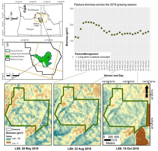
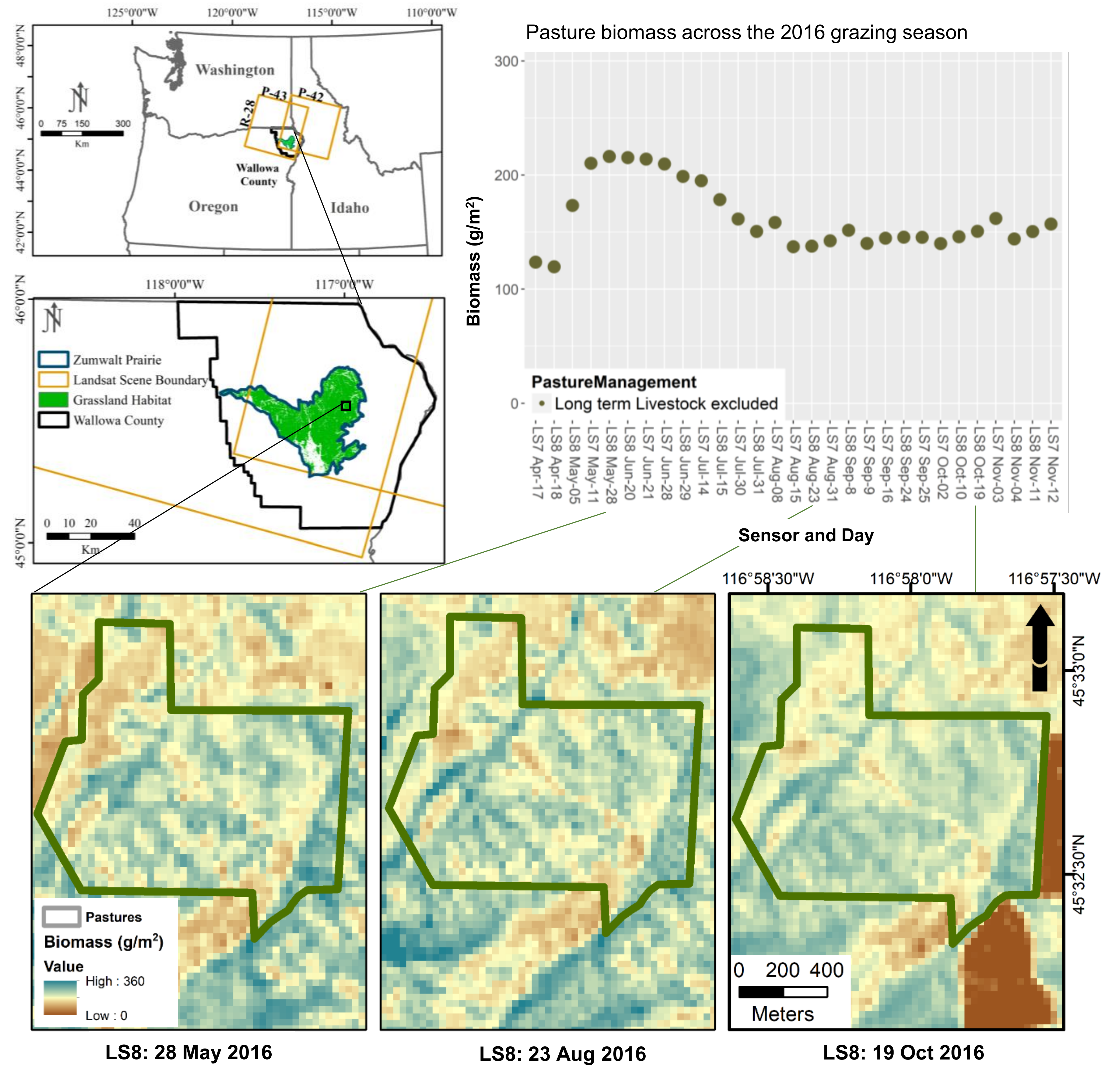
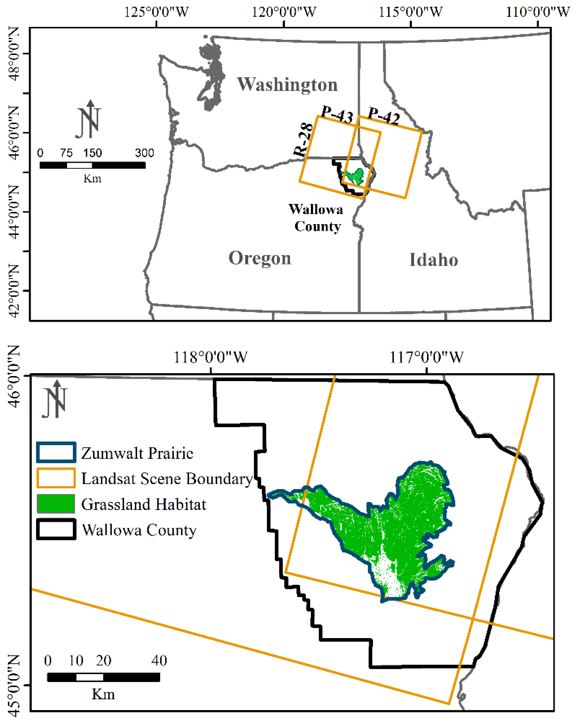
2.1. Study Area

The study area covers approximately 26,300 hectares across six different private land holdings on the Zumwalt Prairie in northeastern Oregon (Figure 1). The Zumwalt Prairie is a grassland dominated by C3 grasses including Idaho fescue (Festuca idahoensis Elmer), bluebunch wheatgrass (Pseudoroegneria spicata (Pursh) A. Love), and Sandberg’s bluegrass (Poa secunda J. Presl). Average yearly rainfall is 352 mm, with 42% coming between 1 April and 1 July; average monthly temperatures range from −3.3 °C in January to 17.8 °C in July (Zumwalt Weather Station 2006–2017 data, https://www.conservationgateway.org). Most soils are classified as xerolls, with parent material coming from basalt, loess, and colluvium [36].

2.2. Sampling Design

Field data was collected over three years (2014 to 2016) across a suitable habitat sampling area on the Zumwalt prairie. The suitable habitat area was delineated by excluding (1) nongrassland habitat types (developed, agriculture, rock, or forest) as defined by the ReGap Ecological Systems data [37]; (2) slopes greater than 45%; and (3) any area falling within 50 m of stock ponds, roads, and fence lines. Sample sites were located at least 200 m away from other sites for each field campaign, and for efficiency purposes, sites were located within 1.1 km of access roads. The sample site locations were located using a stratified random sampling approach generated iteratively for each season and year. Sampling strata were divided by quartiles of predicted biomass amounts derived initially using vegetation models created for this study area [21] and then subsequently updated as new data were collected and analyzed for each season. This stratification was performed for more informed and efficient sampling across a gradient of vegetation amounts. Sites were located within relatively homogenous areas of vegetation and in pastures with various levels of stocking, timing of grazing, and grazing rotation strategies. Sampling was performed at two dominant phenological time periods: during peak biomass (i.e., summer, when green vegetation is dominant) in 2015 and 2016, and during full senescence (i.e., autumn, when brown vegetation is dominant) in 2014, 2015, and 2016.

2.3. Data

2.3.1. Field Data

During the study period (2014–2016), data on standing crop biomass, vegetation cover, soil surface, and utilization were collected at total of 272 sample sites. Field data was collected across three parallel 60-m transects located 30 m apart and oriented east to west with the middle 60-m transect intersecting the site center (Supplemental Materials Figure S1). Vegetation cover, color/condition (i.e., green/photosynthetically active, brown/senesced, and grey/standing dead) and soil surface data were collected every meter across all transects using line–point intercept [38], providing 180 measures per site. Total above-ground biomass was collected using an adapted photo-enhanced comparative yield method described by Friedel and Bastin [39]. Our method involved field observers estimating dry vegetation weight using photographic standards obtained across the Zumwalt Prairie. Biomass collection at each sample site was performed using the photo standards to estimate the weight of standing crop within 39 1.0 × 0.4 m quadrats located every 5 m along each transect. We corrected the field estimated biomass by creating individual observer calibration equations for each year and seasonal data collection bout. This was done by clipping standing crops at four quadrats (at 30 m along the northern and southern transect and 20 m and 40 m along the middle transect) to 0.5 cm above ground surface, and oven drying at 60 °C for 48 h to obtain a dry weight. For each observer, calibration equations were then created using the estimated plot weight and the actual clipped weight. The resulting equations were then applied to each observer’s estimate. Utilization was also assessed at each 1 × 0.4 m quadrat in unison with biomass estimates by visually estimating the amount of vegetation removed by grazing animals. The methods followed double-weight sampling described by Parsons et al. [40].

2.3.2. Remotely Sensed Data

The climate data record (CDR) Collection 1 Level 2 products for Landsat 7 ETM+ and Landsat 8 Operational Land Imager (OLI) were downloaded from USGS Earth Explorer (https://earthexplorer.usgs.gov/, accessed 5 December 2017). Each scene is terrain-corrected and processed to at-surface reflectance based on the sensor type; Landsat 7 ETM+ data is processed with the Landsat Ecosystem Disturbance Adaptive Processing System (LEDAPS) algorithm [41] and Landsat 8 OLI with the Landsat 8 Surface Reflectance Code (LaSRC) [42]. This data product also includes a pixel quality assurance (pixel_qa) band derived largely from the CFMask algorithm [43], which was used to filter pixels containing clouds or shadows over the study site. The location of this study area falls on swath edge paths, enabling each Landsat sensor to pass over every 8 days, and providing Landsat 7 and Landsat 8 scene acquisitions one day apart (e.g., [22]). We selected images that were mostly cloud-free and closest in date to the field campaigns which also had a one-day paired sensor scene (Supplemental Materials Table S1). The paired scenes facilitated a comparison of modeled biomass and cover between sensors. For each of the selected scenes, we masked out bad data by applying the pixel_qa mask. This included the no-data pixels associated with the permanent failure of the Landsat 7 ETM+ scan line corrector in 2006, as well as clouds and shadows across both Landsat 7 and Landsat 8 datasets. For one scene, imaged on 17 October 2015 from Landsat 8, we further applied a manual cloud mask due to error of omission with the pixel_qa mask. Next, we obtained the common spectral bands, and computed 12 vegetation indices and the wetness, greenness, and brightness tasseled cap transformation [44] using the coefficients for reflectance data [45] (Supplemental Materials Table S2) based on previous studies across grassland and dryland systems. For each field sample site, we averaged pixel values across a 2 × 2 pixel window surrounding the sample site to fully capture the field site extent, as the field sites did not fall directly within individual pixels.

2.4. Statistical Analysis

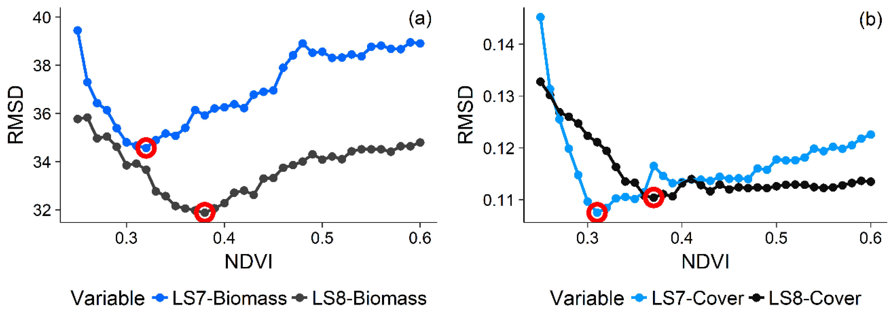
2.4.1. Variable Selection

Using a best-subset regression modeling approach [21,46], we determined which spectral indices (Supplemental Materials Table S2) were most commonly selected for a defined number of variables [46] when estimating vegetation biomass and cover for nine different data combinations based on the sensor and time of year (sensor-time). The best-subset approach exhaustively searches all possible single and multiple variable linear models (with model size defined by the user) and selects the models with the best fit [46]. The sensor–time data combinations consisted of three sensor groupings (Landsat 7, Landsat 8, and Landsat 7/8 combined) and three time groupings that aligned with the dominant phenological periods: peak biomass (i.e., summer, when green vegetation is dominant), full senescence (i.e., autumn, when brown vegetation is dominant), and the combined dataset (i.e., all year). To limit the influence that outlier observations can have on variable selection for each of the nine sensor–time combinations, we ran 1000 iterations, guided by Crowley [47], of a random selection with replacement of two-thirds of the data and performed a best-subset regression (regsubsets in the leaps package in R) [48,49] for each run. We then summed the predictor variables selected as “best” across the 1000 runs to guide the creation of candidate models for each combination.

2.4.2. Model Creation

For each of the nine sensor–time data groups, we divided the valid sample sites into training and testing sets by selecting 75% of the data for training and leaving 25% out for testing. Using the variables selected as “best” from the previous variable selection step (see Section 2.4.1), coefficients for each candidate model were obtained by averaging the coefficient values from 1000 linear models built by randomly selecting two-thirds of the training data for each model run. Using these coefficients, we then created linear models and computed measures of model performance (i.e., relative root mean squared error (rRMSD) and root mean squared deviation (RMSD) [50]) for both the training and testing datasets. Linear model residuals were tested for normality using the Lilliefors test [51] and visually inspected for homoscedasticity. When candidate models had more than one predictor variable, the variance inflation factor (VIF) was calculated. Guided by Graham [52], only candidate models with a VIF of less than 2 were considered for further analysis. From the candidate models, we selected the “best” model as the ones that most consistently had the lowest model errors, while giving priority to vegetation models that contained the same spectral variables across the three sensor data groups for each dominant phenological time period.

2.4.3. Model Comparison across Landsat 7 and Landsat 8 Scenes for Summer and Fall

Once the best model was selected for each of the 9 sensor–time data groups, we compared modeled vegetation amounts between models by applying each model to the paired Landsat 7 and Landsat 8 scenes. We did this for the summer and fall time periods separately due to notable increases in accuracy when modeling the summer vegetation data separately from the fall data. By separating the data in this way, there are nine comparisons when applying each model to each scene (Supplemental Materials Figure S2, step 4: all combinations explored). Across the study area for each scene and model combination, a relative difference raster was calculated as:
% RelDif = ((x − y)/((x + y)*0.5)*100)
where x represents the modeled vegetation amount derived from Landsat 8 scene data and y represents the modeled vegetation amount derived from Landsat 7 data. Next, to minimize the effect of forward and back-scatter, we combined all paired scene pixel differences for the summer and fall periods for a total dataset comparison. We computed the median and mean percent relative differences for each of the six scene date comparisons for each temporal period as well as averages across the six scenes for both the summer and fall periods.

2.4.4. Exploring Pixel-Wise Phenology-Driven Model Application

Due to the impact that vegetation phenology has on accurately estimating vegetation amounts with remotely sensed data [21,53,54] and the desire to automate the application of the appropriate phenological models across the grazing season, we estimated vegetation amounts using an ‘if-else’ statement, whereby if the sampling site value of the NDVI is greater than x, apply the summer model, else apply the fall model. To determine the threshold for each metric (biomass or cover) and sensor, we created a sequential range of NDVI values from 0.25 to 0.60 with a 0.01 step and applied our ‘if-else’ statement to predict a vegetation amount for each site. This sequential range of NDVI values was based on the overlapping span of NDVI values from the summer and fall sampling (Supplemental Materials Figure S5h). For each sensor and vegetation (cover and biomass) dataset and NDVI value between 0.25 and 0.60, we randomly selected 75% of the data and computed measures of model performance (rRMSE and RMSD) on the estimated versus the observed data, with 500 iterations. We averaged measures of model performance across all 500 runs and selected the thresholds that minimized the RMSD. We then compared the three ways to model vegetation across the year with (1) the nonautomated application of summer and fall models based on season; (2) the automated application of models based on phenology (i.e., NDVI threshold); and (3) the consistent application of the all-year models, with the full datasets of Landsat 8 and Landsat 7 separately for each vegetation metric (i.e., cover and biomass).

2.4.5. Analysis of Model Residuals

To understand what physical, environmental, or sampling components most likely influence model error in the cover and biomass threshold algorithms, we correlated the algorithm residuals to ancillary environmental, topographic, in-field, and sensor data using the Spearman’s rank method. Variables related to the sensor and sampling included: in-field sample date (i.e., Julian day), sensor date, number of days between field data collection date and scene acquisition date (days off), and number of days since last measured rainfall prior to overpass. Ecological variables collected at the site included percent foliar cover by plant functional group (perennial grass, perennial forb, annual grass, annual forb) and litter cover. Other data included soil surface variables when no canopy was observed, such as percent soil, moss and lichen cover, and rock. We also further explored the impacts of vegetation color (green, brown, standing dead (grey)) as well as an estimate of percent utilization collected at each sample site. The topographic variables, slope and aspect, were derived from the 30-m national elevation dataset (NED) and averaged across a 2 × 2-pixel window to match the scale of the remotely sensed data (Supplemental Materials Table S3).

3. Results

3.1. Biomass and Cover Field Data

Across the 272 field sites visited during the study period, the average biomass was 133.23 g/m2 and the average percent foliar cover was 0.56%. Biomass and cover data collected in summer exhibited greater average vegetation amounts when compared to data collected in the fall (Table 1). Our sampling design captured a gradient of vegetation amounts exhibited by the high range in biomass and cover amounts for both the summer and fall datasets.

3.2. Variable Selection

The “best” predictor variables selected from the bootstrapped best-subset regression were relatively consistent between Landsat 7 and Landsat 8 across the three time data groupings. For the summer datasets, across all sensor groupings, the variables selected most for cover and biomass were the normalized difference infrared index 7 (NDII7) and the normalized difference water index (NDWI). When exploring the summer datasets with two-variable models, the NDII7 variable was most often selected, but the second variable varied between the sensor groups and the vegetation metric (Supplemental Materials Tables S4 and S7). For both the fall and all-year (summer + fall) data, across all sensor groupings, the normalized difference tillage index (NDTI) was selected as the best predictor variable, while the NDII7 was selected as the second-best predictor (see Supplemental Materials Figures S3–S5 for scatterplots). The variables selected most for the two-variable models differed between the fall and the all-year datasets. The two-variable fall models contained the NDTI variable within each model, with the second variable again varying across the vegetation metric and sensor group. The all-year two-variable models for cover and biomass relied most heavily on the NDTI, NDII7, and to a lesser extent the NDWI (Supplemental Materials Tables S4–S9).

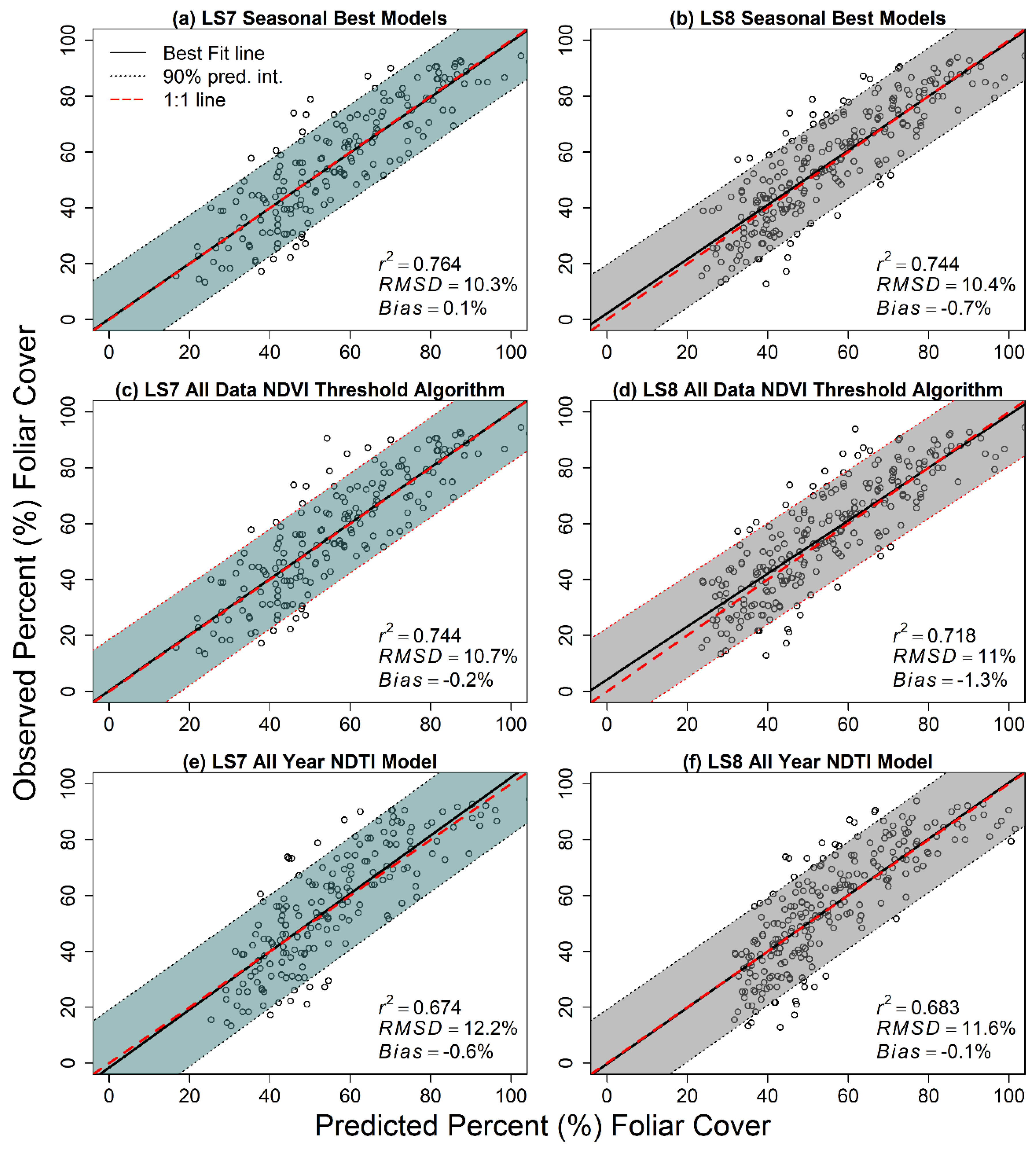
3.3. Candidate Model Comparisons and Model Selection

Across all three time periods analyzed, the two-variable models with variance inflation factors (VIF) under two did not consistently (across training and testing datasets) outperform the one-variable models by more than 1.5% rRMSE, or more than 1% for cover, or 1 g for biomass RMSD (Supplemental Materials Tables S10 and S11). The highest-ranked one-variable models for each time and sensor combination were all significant, with coefficients of determination (r2) ranging from 0.65 to 0.81, and with rRMSE ranging from 13.00% to 30.88%.
Since the NDII7-based models had the lowest predictor error across the majority of the summer cover and biomass modeling datasets, we selected the NDII7 models for further analysis. The NDII7 models for cover had rRMSE values less than 18% and RMSD values less than 11% (r2 > 0.70), with similar model evaluation statistics observed between the training and testing datasets. For biomass, model evaluation statistics for the training data had rRMSE values less than 23% and RMSD values less than 40 g/m2 (r2 > 0.69), while the testing dataset had lower rRMSE values (<21.5%) and RMSD values (<35 g/m2) and higher r2 coefficients (>0.8) (Table 2).
Across the fall and all-year datasets, the NDTI-based models were selected because this predictor minimized errors across every sensor group for both cover and biomass when compared to the other one-variable models. For fall cover data, the NDTI-based models had r2 values greater than 0.72, with rRMSE values less than 23% and RMSD values less than 13%. For fall biomass data, the NDTI based models had r2 values greater than 0.67, with rRMSE under 31% and RMSD under 33 g/m2. Including both the summer and fall data together for the all-year datasets, the NDTI biomass models had r2 values ranging from 0.67 to 0.77, with rRMSE less than 30% and RMSD ranging from 35.11 to 40.52 g/m2. Cover NDTI models had r2 values ranging from 0.65 to 0.72, with rRMSE less than 23% and RMSD ranging from 0.12 to 0.13%.
The relative root mean squared errors (rRMSE) were smaller on average when modeling summer vegetation datasets as compared to modeling the fall vegetation data, and the vegetation cover metric had lower rRMSE values compared to the biomass metric. While the rRMSE values were lower for the summer dataset, this pattern was not observed with the RMSD statistic for the biomass metric, which showed improvements in prediction accuracy for the fall data versus the summer data across all sensor groups and testing and training datasets, except the LS8 testing dataset.
When removing all sampling locations which were only valid for one sensor, so that we could compare model accuracy between sensors using an identical dataset of field data, we observed that for vegetation cover, the Landsat 7 and Landsat 8 data products provide very similar model fit estimates (i.e., within 1.5% rRMSE of each other) across all three temporal datasets (summer, fall, all year). When modeling summer biomass, the Landsat 8 sensor-based model was more accurate than the Landsat 7 biomass model, having a lower rRMSE of 3% and 2% with the training and testing data, respectively. When modeling the fall biomass data, the Landsat 7 biomass model reduced errors when compared to the Landsat 8-based model, with a 0.5% and 3% reduction of the rRMSE with the training and testing data, respectively (Supplemental Materials Tables S12 and S13).

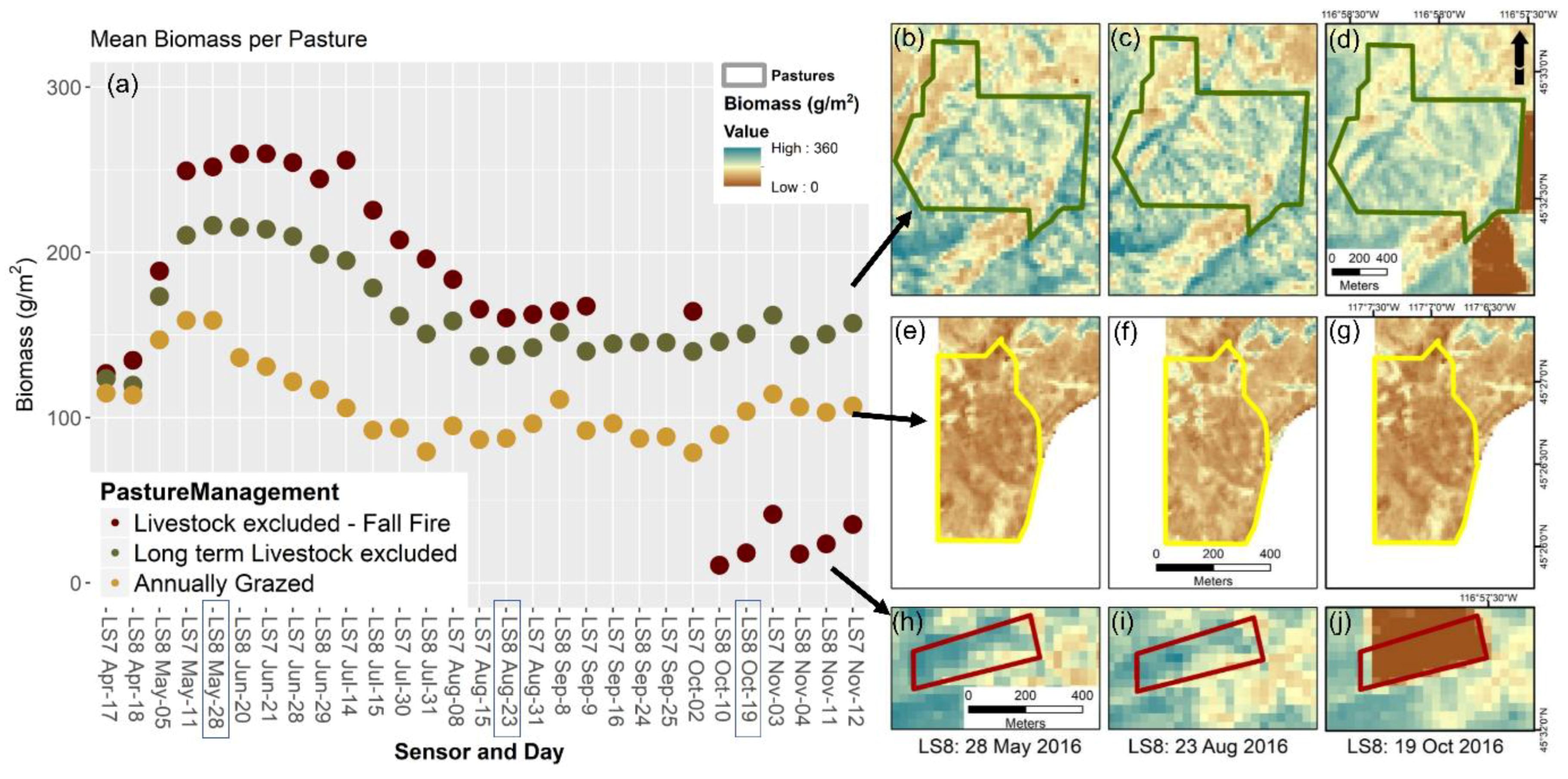
3.4. Relative Differences in Modeled Vegetation across Paired Landsat 7 and Landsat 8 Scenes

The cover and biomass vegetation models that aligned to each sensor (sensor-aligned models; i.e., applying the Landsat 8 model to Landsat 8 data) had the smallest differences between estimated vegetation across the scene pairs for both summer and fall (Figure 2 and Figure 3). For biomass, applying the sensor-aligned models across the six summer scene pairs resulted in a range of median percent relative differences from −2.73% (Landsat 7 bias) to 2.63% (Landsat 8 bias) with an average median percent relative difference of 0.33%. Across the six fall scenes, using the sensor-aligned biomass models, the median percent relative differences ranged from −4.54% to 3.55% with an average median percent relative difference of −0.39% (Supplemental Materials Table S14). These results are similar to the sensor-aligned cover models for both summer (median range = −1.62% to 2.00%, average median = 0.49%) and fall (median range = −3.87% to 2.21%, average median = −0.58%) (Supplemental Materials Table S15).
Across the six summer scene pairs, we observed a positive bias (average median percent relative difference of +2.22%) in NDII7 values from Landsat 8 as compared to Landsat 7. Across the six fall scene pairs, we observed a small negative bias (average median percent relative difference of −1.16%) in NDTI values with Landsat 8 data as compared to Landsat 7. Applying the sensor-data aligned models to the Landsat 7 and Landsat 8 data decreased sensor bias for the resulting vegetation amounts in both the summer and fall time periods (Supplemental Materials Tables S14 and S15).

3.5. Assessing a Pixel-Wise Phenologically (NDVI) Driven Model Application across the Grazing Season

The NDVI threshold values that guide application of season-specific models for biomass were 0.38 and 0.32 for Landsat 8 and Landsat 7 data, respectively. Cover thresholds were very similar to that of biomass, with the RMSD minimized at NDVI values of 0.37 for Landsat 8 data and 0.31 for Landsat 7 data (Figure 4).
The RMSD varied less than 1.5 g/m2 for biomass (Figure 5) and less than 1% for cover (Figure 6) when comparing the season-specific model (Figure 5a,b and Figure 6a,b) to the NDVI-threshold algorithm method (Figure 5c,d and Figure 6c,d). The all-year NDTI-based models (Figure 5e,f and Figure 6e,f) also performed well, but had the largest RMSD across both sensors and vegetation metrics when compared to the other two methods of applying the models’ Landsat data.

3.6. Correlation of NDVI Threshold Model Error with Sensor, Sampling, and Field Variables

For both the cover and biomass metrics, the maximum significant correlation had an absolute correlation coefficient (r) of 0.41. Only percent perennial grass, percent litter, prior rain events, and percent moss and lichen had r values over 0.30 for any sensor/vegetation metric (Table 3).

4. Discussion

To provide near real-time data for adaptive management, we developed and tested an approach to automate the quantification and mapping of vegetation cover and biomass using Landsat 7 and Landsat 8 CDR products across the grazing season (i.e., changing phenological conditions) by relying on NDVI thresholds to guide season-specific model application. We showed that using NDVI to select from seasonal models for application increased accuracies when modeling vegetation amounts at varying growth stages compared to the single variable all-year NDTI models. Our finding that Landsat 8 has a larger NDVI threshold value as compared to Landsat 7 aligns with previous literature that found that Landsat 8-derived NDVI values are greater than those of Landsat 7 [22,23]. These sensor-specific algorithms enable efficient mapping, analysis, and accessibility of biomass and cover estimates throughout the grazing season as vegetation changes due to phenology and management. This is a substantial improvement over point-based quantitative observations or plot-based qualitative assessments. The vegetation maps provide a richer, more complete representation of vegetation amounts for land managers and ranchers to use in assessing the outcomes of their management actions. One example application of this model at the pasture scale reveals the differences in biomass corresponding to various management strategies (Figure 7).
Our results from season-specific modeling, using data from the summer sampling period, determined that NDII7 was the most accurate spectral predictor of biomass and cover; this is in contrast to the wide use of NDVI as a proxy for rangeland vegetation [55]. We attribute this result to the fact that over one-third of our summer sampling sites had more than 30% brown or standing dead vegetation cover, since the relationship between total biomass and NDVI is affected by the amount of standing dead (prior year’s growth) or senescent (current year’s growth that is no longer photosynthetically active) vegetation [27]. Furthermore, in rangelands where species diversity and heterogenous soil conditions create high phenological variability within a single pixel as well as over the study area, the impact of nonphotosynthetically active vegetation is especially important to take into account when modeling vegetation metrics for rangeland monitoring [28,31].
For the fall sampling period, the best predictor (NDTI) contained the two shortwave infrared bands, which correlate to cellulose and lignin in vegetation [29,30,56]. Vegetation indices such as the soil tillage index (STI), the normalized difference tillage index (NDTI), and the soil adjusted total vegetation index (SATVI), which rely in part on the shortwave infrared (SWIR) bands, have been used to estimate dry vegetation and total vegetation in semiarid rangelands across the African Sahel [30], the southwest USA [19,31], and photosynthetic and nonphotosynthetic vegetation across the Australian savanna [57]. Our ability to explain the variance of dry vegetation amounts in both cover and biomass is comparable and slightly better than that of Jacques et al. [30], who found an r2 of 0.67 when linearly relating biomass and STI across the year, an r2 of 0.59 when using only the dry season measures, and an r2 of 0.66 during the wet season. We attribute this slight improvement to our dataset containing fewer years’ data, being collected across a smaller, more similar habitat type, and the higher spatial resolution of Landsat compared to MODIS. Furthermore, compared to Jansen et al. [21], we observed improved model accuracy as well as simplified models (one-variable models compared to multivariable models). Model improvement is especially evident for the fall biomass models, exhibited by an increase of the r2 from 0.35 in Jansen et al. [21] to 0.67 in this study. This is likely due to our larger in-field plot size, improved in-field biomass estimates, as well as the fact that we sampled a greater range of vegetation amounts and had a much larger sample size. Similar to Jacques et al. [30], NDTI also performed quite well across both the summer and fall periods of this study. These findings support the idea that SWIR vegetation indices are sensitive to both green and brown vegetation [58] in grassland systems with darker soil. The parent material that makes up the Zumwalt Prairie soils comes from basalt and loess, creating dark soils in contrast to the bright soils of the Sahel [30].
Comparing the relative differences between paired scenes showed that sensor-specific models decreased differences in predicted vegetation amounts between Landsat 7 and Landsat 8 scenes. Across the Zumwalt study area, we observed a small positive bias with the Landsat 8 summer time NDII7 (also known as the Normalized Burn Ratio (NBR)) and a small negative bias with the Landsat 8 fall NDTI (Supplemental Materials Tables S14 and S15). Using sensor-specific models for vegetation biomass and cover eliminates the need to normalize images across the image analysis stack [23]. While we observed reduced bias between scenes with sensor-specific models, the individual scene pair comparisons did vary, with bias not always trending in the same direction for each Landsat 7/Landsat 8 scene pair. This is likely due to differences in atmospheric effects and pixels missed by the pixel quality assurance (pixel_qa) mask that contained clouds, shadows, and aerosols. For example, we had to apply a manual cloud mask to the 17 October 2015 scene, due to errors of omission of the pixel_qa mask with high cirrus clouds and shadows. Such errors can lead to spurious results, necessitating the collection of field data across many years [21] and careful screening of scenes to effectively remove spurious data due to clouds, shadows, and aerosol effects [22] for more accurate models and their associated vegetation products.
Another important aspect of understanding the accuracy of these models for decision-making tools is assessing where or when they may produce unreliable estimates. Places where the model tended to underestimate vegetation amounts were in highly productive areas of deep soil with dense, multi-layered vegetation canopies (potentially due to shadowing), areas where annual grass has filled interspaces between bunchgrasses, and areas of dense, continuous annual grass cover (Figure 8). Further evidence of this underestimation is our finding that both perennial and annual grass cover were negatively correlated to model residuals.
Overestimation seemed to be associated with several different factors. Sites where the models tended to overpredict vegetation amounts, especially vegetation cover, were in areas with high vegetation heterogeneity, such as on mima mounds [59] or areas with greater rock cover (Figure 9).
Cover and biomass on sites with a greater percentage of moss/lichen cover also tended to be overestimated. This aligns with Rodriquez-Caballero et al. [60], who found that NDVI and the enhanced vegetation index (EVI) were impacted by biological crust cover, resulting in higher vegetation index values. Litter cover was another factor contributing to overestimation, which is likely due to the models and associated vegetation indices not being sensitive to the difference between attached and unattached plant material. Litter has been cited as a source of error when estimating biophysical parameters in grassland systems [25]. The NDII7 and NDTI vegetation indices used to model cover and biomass are sensitive to both green and brown plant material [58,61,62], such as crop residue, because the SWIR band (around 2100 nm) effectively differentiates plant material (cellulose and lignin) from soil [29,63,64]. Overestimation observed with rain lag is likely due to the SWIR bands also being sensitive to water content [63,65], with greater reflectance occurring with drier conditions as opposed to greater absorption with more moisture [65,66,67].
This study revealed challenges and tested the feasibility of using Landsat’s surface reflectance products to model vegetation amounts that are applicable to rangeland management across the grazing season. Improvements can be made with more technical and automated cloud and shadow filtering. For example, Roy et al. [22] used the blue-band filter to remove pixels with significant surface change from the image pair. Exploring different modeling methods such as random forests [68], artificial neural networks (e.g., [69]), or support vector machines [70] may improve model accuracy. We did explore improving the model accuracy of cover data with quadratic polynomial models and found that they did not decrease the rRMSE by more than 1% consistently across the training and testing sets (Supplemental Materials Figure S6 and Table S16). Combining remotely sensed datasets such as Landsat and Sentinel-2, which has a global median average revisit time of less than three days [71], would allow for further improvement of near real-time multitemporal monitoring of vegetation at management scales. Other options would be to use fusion algorithms relying on MODIS data, such as the spatial and temporal adaptive reflectance fusion model, StarFM [72], or the spatial temporal adaptive algorithm for mapping reflectance change (STAARCH) [73]. Remote sensing science and availability of data products in GEE will continue to improve, making it increasingly realistic to deliver accurate data in near real-time to decision-makers.
To date, one of the biggest obstacles facing rangeland ecologists is consistently sharing information derived from remotely sensed analysis with managers and ranchers. We are utilizing GEE by leveraging the ClimateEngine [35] to distribute these modeled cover and biomass vegetation products to stakeholders in a timely, cost-effective, and automated way. One of the initial goals of this research was to provide accessible, timely, and zero-cost estimates of vegetation amounts across the grazing season to enable adaptive management and monitoring at the pasture, ranch, and landscape scale. A landscape-wide vegetation dataset such as this one can provide consistent unbiased data for making comparisons and sharing successful management strategies across property lines over time. As climate change continues to amplify the annual and interannual variability in rangeland ecosystems [9], sharing successful adaptation and management strategies between ranchers and researchers will become increasingly necessary [74]. The analyses undertaken here support tool development by (1) testing the sensitivity of models across sensors and across the grazing season (2) and by empirically identifying a threshold for phenologically aligned model application.

5. Conclusions

Near real-time estimates of vegetation cover and biomass are critical to adaptive rangeland management. NDVI has been widely used for rangeland monitoring tools and can provide a rough proxy of vegetation production and phenology, but is less accurate when vegetation contains high proportions of standing dead or senescent vegetation. Developing phenology-driven predictive models specific to each Landsat 7 and 8 CDR product yielded consistent and nonbiased estimates of total vegetation cover and above-ground biomass across the grazing season. Applying these models in Google Earth Engine provides a platform for land managers and ranchers to utilize timely, cost-effective, and unbiased information to meet objectives and improve outcomes. We suggest that future ecological applications of remote sensing products that are developed with Google Earth Engine or other platforms should also seek to incorporate seasonality into product development and conduct sensitivity analyses, and validate the models with field data to ensure accurate performance under short- and long-term dynamic vegetation conditions.

Supplementary Materials

The following are available online at https://www.mdpi.com/2072-4292/10/7/1057/s1, Figure S1: Sampling site plot layout, Table S1. Paired Landsat 7 and Landsat 8 scenes used in model building (including timing of in-field vegetation sampling) and for sensor model comparisons, Table S2. Candidate vegetation indices used in the best subset modeling step, Figure S2. Workflow diagram for final algorithm development, Table S3. The field, sensor and topographic variables used to correlate with residuals from the NDVI threshold algorithm, Table S4. Variable Selection using a bootstrapped best subset model approach for green (summer) biomass data, Table S5. Variable Selection using a bootstrapped best subset model approach for brown (fall) biomass data, Table S6. Variable Selection using a bootstrapped best subset model approach for All Year (Green + Brown) biomass data, Table S7. Variable Selection using a bootstrapped best subset model approach for green (summer) cover data, Table S8. Variable Selection using a bootstrapped best subset model approach for the fall (brown) cover data, Table S9. Variable Selection using a bootstrapped best subset model approach for the complete dataset (All Year) cover data, Table S10. Top candidate models for Cover, Table S11. Top candidate models for Biomass, Table S12. Paired Cover models, Table S13. Paired Biomass models, Figure S3. Scatter plots between in-field estimates of cover and biomass with select vegetation indices (NDTI, NDII7, NDVI) using Landsat 7 data. Figure S4. Scatter plots between in-field estimates of cover and biomass with select vegetation indices (NDTI, NDII7, NDVI) using Landsat 8 data. Figure S5. Scatter plots between in-field estimates of cover and biomass with select vegetation indices (NDTI, NDII7, NDVI) using Landsat 7 and Landsat 8 data. Table S14. Table of Median and Mean pixel differences in Biomass across scene pairs across all model combinations and the associated vegetation index (NDII7 for Green, NDTI for Brown), Table S15. Table of Median and Mean differences in Cover between scene pairs across all model combinations and the associated vegetation index (NDII7 for Green, NDTI for Brown), Figure S6. Scatter plots of simple and polynomial linear regressions using the summer, fall, and all-year cover data for both Landsat 7 and Landsat 8, Figure S16. Model fit statistics for simple and polynomial linear regressions using the summer and fall cover data. References [75,76,77,78,79,80,81,82,83,84,85] are cited in the supplementary materials.

Author Contributions

V.S.J. and C.A.K. conceptualized this research paper, with V.S.J. and H.J.S. leading the field work; V.S.J. performed the formal analysis, with H.J.S. performing in-field assessment and validation of the end biomass and cover products. V.S.J. led the manuscript writing with C.A.K. and H.J.S. providing reviewing and editing.

Funding

This research was funded by the Priscilla Bullitt Collins Trust Northwest Conservation Fund and The Nature Conservancy.

Acknowledgments

The authors would like to thank the people at ClimateEngine, specifically Katherine Hegewisch, for all the tool development; all the individuals who assisted with the collection of field data; as well as Robert V. Taylor for his vision and insight and Jason Dingeldein for guidance and encouragement. We also thank Jeff Fields and Derek Johnson, and the Oregon Chapter of TNC for support. Lastly, the authors thank the four anonymous reviewers for comments that improved the manuscript.

Conflicts of Interest

The authors declare no conflict of interest.

References

  1. Asner, G.P.; Elmore, A.J.; Olander, L.P.; Martin, R.E.; Harris, T.A. Grazing Systems, Ecosystem Responses, and Global Change. Annu. Rev. Environ. Resour. 2004, 29, 261–299. [Google Scholar] [CrossRef]
  2. Fleishchner, T.L. Ecological Costs of Livestock Grazing in Western North America. Soc. Conserv. Biol. 1994, 8, 629–644. [Google Scholar] [CrossRef]
  3. Brunson, M.W.; Huntsinger, L. Ranching as a Conservation Strategy: Can Old Ranchers Save the New West? Rangel. Ecol. Manag. 2008, 61, 137–147. [Google Scholar] [CrossRef]
  4. Sullins, M.J.; Theobald, D.T.; Jones, J.R.; Burgess, L.M.; Knight, R.L.; Gilgert, W.C.; Marston, E. Lay of the Land: In Ranching West of the 100th Meridian: Culture, Ecology, and Economics; Island Press: Washington, DC, USA, 2002; ISBN 1-55963-826-5. [Google Scholar]
  5. Sayre, N.F.; McAllister, R.R.; Bestelmeyer, B.T.; Moritz, M.; Turner, M.D. Earth Stewardship of rangelands: Coping with ecological, economic, and political marginality. Front. Ecol. Environ. 2013, 11, 348–354. [Google Scholar] [CrossRef]
  6. Huntsinger, B.L.; Sayre, N.F. Introduction: The Working Landscapes Special Issue. Rangelands 2007, 29, 3–4. [Google Scholar] [CrossRef]
  7. Stafford Smith, D.M.; McKeon, G.M.; Watson, I.W.; Henry, B.K.; Stone, G.S.; Hall, W.B.; Howden, S.M. Learning from episodes of degradation and recovery in variable Australian rangelands. Proc. Natl. Acad. Sci. USA 2007, 104, 20690–20695. [Google Scholar] [CrossRef] [PubMed] [Green Version]
  8. Mckeon, G.; Day, K.; Howden, S.; Mott, J.; Orr, D.; Scattini, W.; Weston, E. Australian savannas: Management for pastoral production. J. Biogeogr. 1990, 17, 355–372. [Google Scholar] [CrossRef]
  9. Joyce, L.A.; Briske, D.D.; Brown, J.R.; Polley, W.H.; McCarl, B.A.; Bailey, D.W. Climate Change and North American Rangelands: Assessment of Mitigation and Adaptation Strategies. Rangel. Ecol. Manag. 2013, 66, 512–528. [Google Scholar] [CrossRef] [Green Version]
  10. Sayre, N.F.; deBuys, W.; Bestelmeyer, B.T.; Havstad, K.M. “The Range Problem” After a Century of Rangeland Science: New Research Themes for Altered Landscapes. Rangel. Ecol. Manag. 2012, 65, 545–552. [Google Scholar] [CrossRef]
  11. Bestelmeyer, B.T.; Briske, D.D. Grand Challenges for Resilience-Based Management of Rangelands. Rangel. Ecol. Manag. 2012, 65, 654–663. [Google Scholar] [CrossRef]
  12. Washington-Allen, R.A.; West, N.E.; Ramsey, R.D.; Efroymson, R.A. A Protocol for Retrospective Remote Sensing—Based Ecological Monitoring of. Rangel. Ecol. Manag. 2006, 59, 19–29. [Google Scholar] [CrossRef]
  13. Briske, D.D.; Fuhlendorf, S.D.; Smeins, F.E. State-and-Transition Models, Thresholds, and Rangeland Health: A Synthesis of Ecological Concepts and Perspectives. Rangel. Ecol. Manag. 2005, 58, 1–10. [Google Scholar] [CrossRef]
  14. Pyke, D.; Herrick, J.; Shaver, P.; Pellant, M. Rangeland health attributes and indicators for qualitative assessment. J. Range Manag. 2002, 55, 584–597. [Google Scholar] [CrossRef]
  15. Weltz, M.A.; Dunn, G.; Reeder, J.; Frasier, G. Ecological Sustainability of Rangelands. Arid L. Res. Manag. 2003, 369–388. [Google Scholar] [CrossRef]
  16. West, N.E. History of Rangeland Monitoring in the USA. Arid Land Res. Manag. 2003, 17, 495–545. [Google Scholar] [CrossRef]
  17. Briske, D.D.; Washington-Allen, R.A.; Johnson, C.R.; Lockwood, J.A. Catastrophic Thresholds: A Synthesis of Concepts, Perspectives, and Applications. Ecol. Soc. 2010, 15, 37. [Google Scholar] [CrossRef]
  18. Herrick, J.E.; Lessard, V.C.; Spaeth, K.E.; Shaver, P.L.; Dayton, R.S.; Pyke, D.A.; Jolley, L.; Goebel, J.J. National ecosystem assessments supported by scientific and local knowledge. Front. Ecol. Environ. 2010, 8, 403–408. [Google Scholar] [CrossRef]
  19. Hagen, S.C.; Heilman, P.; Marsett, R.; Torbick, N.; Salas, W.; van Ravensway, J.; Qi, J. Mapping Total Vegetation Cover across Western Rangelands with Moderate-Resolution Imaging Spectroradiometer Data. Rangel. Ecol. Manag. 2012, 65, 456–467. [Google Scholar] [CrossRef]
  20. Ikeda, H.; Okamoto, K.; Fukuhara, M. Estimation of aboveground grassland phytomass with a growth model using Landsat TM and climate data. Int. J. Remote Sens. 1999, 20, 2283–2294. [Google Scholar] [CrossRef]
  21. Jansen, V.S.; Kolden, C.A.; Taylor, R.V.; Newingham, B.A. Quantifying livestock effects on bunchgrass vegetation with Landsat ETM+ data across a single growing season. Int. J. Remote Sens. 2016, 37, 150–175. [Google Scholar] [CrossRef]
  22. Roy, D.P.; Kovalskyy, V.; Zhang, H.K.; Vermote, E.F.; Yan, L.; Kumar, S.S.; Egorov, A. Characterization of Landsat-7 to Landsat-8 reflective wavelength and normalized difference vegetation index continuity. Remote Sens. Environ. 2016, 185, 57–70. [Google Scholar] [CrossRef]
  23. Holden, C.E.; Woodcock, C.E. An analysis of Landsat 7 and Landsat 8 under flight data and the implications for time series investigations. Remote Sens. Environ. 2016. [Google Scholar] [CrossRef]
  24. Butterfield, H.S.; Malmström, C.M. The effects of phenology on indirect measures of aboveground biomass in annual grasses. Int. J. Remote Sens. 2009, 30, 3133–3146. [Google Scholar] [CrossRef]
  25. Xu, D.; Guo, X.; Li, Z.; Yang, X.; Yin, H. Measuring the dead component of mixed grassland with Landsat imagery. Remote Sens. Environ. 2014, 142, 33–43. [Google Scholar] [CrossRef]
  26. Van Leeuwen, W.J.D.; Huete, A.R. Effects of standing litter on the biophysical interpretation of plant canopies with spectral indices. Remote Sens. Environ. 1996, 55, 123–138. [Google Scholar] [CrossRef]
  27. Huete, A.R.; Jackson, R.D. Suitability of spectral indices for evaluating vegetation characteristics on arid rangelands. Remote Sens. Environ. 1987, 23, 213–218. [Google Scholar] [CrossRef]
  28. Todd, S.W.; Hoffer, R.M.; Milchunas, D.G. Biomass estimation on grazed and ungrazed rangelands using spectral indices. Int. J. Remote Sens. 1998, 19, 427–438. [Google Scholar] [CrossRef]
  29. Elvidge, C. Visible and near infrared reflectance characteristics of dry plant materials. Int. J. Remote Sens. 1990, 11, 1775–1795. [Google Scholar] [CrossRef]
  30. Jacques, D.C.; Kergoat, L.; Hiernaux, P.; Mougin, E.; Defourny, P. Monitoring dry vegetation masses in semi-arid areas with MODIS SWIR bands. Remote Sens. Environ. 2014, 153, 40–49. [Google Scholar] [CrossRef]
  31. Marsett, R.C.; Qi, J.; Heilman, P.; Biedenbender, S.H.; Watson, M.C.; Amer, S.; Weltz, M.; Goodrich, D.; Marsett, R. Remote Sensing for Grassland Management in the Arid Southwest. Rangel. Ecol. Manag. 2006, 59, 530–540. [Google Scholar] [CrossRef] [Green Version]
  32. Guerschman, J.P.; Scarth, P.F.; Mcvicar, T.R.; Renzullo, L.J.; Malthus, T.J.; Stewart, J.B.; Rickards, J.E.; Trevithick, R. Assessing the effects of site heterogeneity and soil properties when unmixing photosynthetic vegetation, non-photosynthetic vegetation and bare soil fractions from Landsat and MODIS data. Remote Sens. Environ. 2015, 161, 12–26. [Google Scholar] [CrossRef]
  33. Gorelick, N.; Hancher, M.; Dixon, M.; Ilyushchenko, S.; Thau, D.; Moore, R. Google Earth Engine: Planetary-scale geospatial analysis for everyone. Remote Sens. Environ. 2017, 202, 18–27. [Google Scholar] [CrossRef]
  34. Hansen, M.C.; Potapov, P.V.; Moore, R.; Hancher, M.; Turubanova, S.A.; Tyukavina, A.; Thau, D.; Stehman, S.V.V.; Goetz, S.J.; Loveland, T.R.; et al. High-Resolution Global Maps of 21st-Century Forest Cover Change. Science 2013, 342, 850–854. [Google Scholar] [CrossRef] [PubMed]
  35. Huntington, J.L.; Hegewisch, K.C.; Daudert, B.; Morton, C.G.; Abatzoglou, J.T.; McEvoy, D.J.; Erickson, T. Climate engine: Cloud computing and visualization of climate and remote sensing data for advanced natural resource monitoring and process understanding. Bull. Am. Meteorol. Soc. 2017, 98, 2397–2409. [Google Scholar] [CrossRef]
  36. Schmalz, H.J.; Taylor, R.V.; Johnson, T.N.; Kennedy, P.L.; DeBano, S.J.; Newingham, B.A.; McDaniel, P.A. Soil Morphologic Properties and Cattle Stocking Rate Affect Dynamic Soil Properties. Rangel. Ecol. Manag. 2013, 66, 445–453. [Google Scholar] [CrossRef]
  37. Kagan, J.; Ohmann, J.; Gregory, M.; Tobalske, C.; Hak, J.; Fried, J. Final Report on Land Cover Mapping Methods: Map Zones 8 and 9, PNW ReGAP; Institute for Natural Resources, Oregon State University: Corvallis, OR, USA, 2006. [Google Scholar]
  38. Herrick, J.E.; Van Zee, J.W.; Havstad, K.M.; Burkett, L.M.; Whitford, W.G.; Pyke, D.A.; Remmenga, M.D.; Shaver, P.L. Monitoring Manual for Grassland, Shrubland and Savanna Ecosystems; USDA-ARS Jornada Experimental Range: Las Cruces, NM, USA, 2005; p. 236. [Google Scholar]
  39. Friedel, M.H.; Bastin, G.N. Photographic standards for estimating compariative yield in arid rangelands. Aust. Rangel. J. 1988, 10, 34–38. [Google Scholar] [CrossRef]
  40. Parsons, C.T.; Momont, P.A.; Delcurto, T.; Mcinnis, M.; Porath, L.; Marni, L. Cattle distribution patterns and vegetation use in mountain riparian areas. J. Range Manag. 2003, 56, 334–341. [Google Scholar] [CrossRef]
  41. Masek, J.G.; Vermote, E.F.; Saleous, N.E.; Wolfe, R.; Hall, F.G.; Huemmrich, K.F.; Gao, F.; Kutler, J.; Lim, T. A Landsat Surface Reflectance Dataset. IEEE Geosci. Remote Sens. Lett. 2006, 3, 68–72. [Google Scholar] [CrossRef]
  42. Vermote, E.; Justice, C.; Claverie, M.; Franch, B. Preliminary analysis of the performance of the Landsat 8/OLI land surface reflectance product. Remote Sens. Environ. 2016. [Google Scholar] [CrossRef]
  43. Zhu, Z.; Woodcock, C.E. Object-based cloud and cloud shadow detection in Landsat imagery. Remote Sens. Environ. 2012, 118, 83–94. [Google Scholar] [CrossRef]
  44. Kauth, R.J.; Thomas, G.S. The Tasselled Cap—A Graphic Description of the Spectral-Temporal Development of Agricultural Crops as Seen by LANDSAT. In Proceedings of the Symposium on Machine Processing of Remotely Sensed Data, Purdue University, West LaFayette, IN, USA, 29 June–1 July 1976. [Google Scholar]
  45. Crist, E.P. A TM Tasseled Cap equivalent transformation for reflectance factor data. Remote Sens. Environ. 1985, 17, 301–306. [Google Scholar] [CrossRef]
  46. Hudak, A.T.; Crookston, N.L.; Evans, J.S.; Falkowski, M.J.; Smith, A.M.S.; Gessler, P.E.; Morgan, P. Regression modeling and mapping of coniferous forest basal area and tree density from discrete-return lidar and multispectral satellite data. Can. J. Remote Sens. 2006, 32, 126–138. [Google Scholar] [CrossRef]
  47. Crowley, P.H. Resampling methods for computation-intensive data analysis in ecology and evolution. Annu. Rev. Ecol. Syst. 1992, 23, 405–447. [Google Scholar] [CrossRef]
  48. Thomas, L. R package Version 3.0. Leaps: Regression Subset Selection. 2017. Available online: https://cran.r-project.org/package=leaps (accessed on 4 July 2018).
  49. R Development Core Team. R: A Language and Environment for Statistical Computing; R Found. Stat. Computing: Vienna, Austria, 2016; ISBN 3-900051-07-0. Available online: http://www.R-project.org/ (accessed on 4 July 2018).
  50. Pineiro, G.; Perelman, S.; Guerschman, J.P.; Jose, P.M. How to evaluate models: Observed vs. predicted or predicted vs. observed? Ecol. Modell. 2008, 216, 316–322. [Google Scholar] [CrossRef]
  51. Lilliefors, H. On the Kolmogorov-Smirnov test for normality with mean and variance unknown. J. Am. Stat. Assoc. 1967, 62, 399–402. [Google Scholar] [CrossRef]
  52. Graham, M.H. Confronting multicollinearity in ecological Multiple Regression. Ecology 2003, 84, 2809–2815. [Google Scholar] [CrossRef]
  53. Vescovo, L.; Gianelle, D. Using the MIR bands in vegetation indices for the estimation of grassland biophysical parameters from satellite remote sensing in the Alps region of Trentino (Italy). Adv. Sp. Res. 2008, 41, 1764–1772. [Google Scholar] [CrossRef]
  54. Malmstrom, C.M.; Butterfield, H.S.; Barber, C.; Dieter, B.; Harrison, R.; Qi, J.; Riaño, D.; Schrotenboer, A.; Stone, S.; Stoner, C.J.; et al. Using Remote Sensing to Evaluate the Influence of Grassland Restoration Activities on Ecosystem Forage Provisioning Services. Restor. Ecol. 2009, 17, 526–538. [Google Scholar] [CrossRef]
  55. Svoray, T.; Perevolotsky, A.; Atkinson, P.M. Ecological sustainability in rangelands: The contribution of remote sensing. Int. J. Remote Sens. 2013, 34, 6216–6242. [Google Scholar] [CrossRef]
  56. Roberts, D.A.; Smith, M.O.; Adams, J.B. Green vegetation, nonphotosynthetic vegetation, and soils in AVIRIS data. Remote Sens. Environ. 1993, 44, 255–269. [Google Scholar] [CrossRef]
  57. Guerschman, J.P.; Hill, M.J.; Renzullo, L.J.; Barrett, D.J.; Marks, A.S.; Botha, E.J. Estimating fractional cover of photosynthetic vegetation, non-photosynthetic vegetation and bare soil in the Australian tropical savanna region upscaling the EO-1 Hyperion and MODIS sensors. Remote Sens. Environ. 2009, 113, 928–945. [Google Scholar] [CrossRef]
  58. Renier, C.; Waldner, F.; Jacques, D.C.; Babah Ebbe, M.A.; Cressman, K.; Defourny, P. A dynamic vegetation senescence indicator for near-real-time desert locust habitat monitoring with MODIS. Remote Sens. 2015, 7, 7545–7570. [Google Scholar] [CrossRef]
  59. Cramer, M.D.; Barger, N.N. Are mima-like mounds the consequence of long-term stability of vegetation spatial patterning? Palaeogeogr. Palaeoclimatol. Palaeoecol. 2014, 409, 72–83. [Google Scholar] [CrossRef]
  60. Rodríguez-Caballero, E.; Knerr, T.; Weber, B. Importance of biocrusts in dryland monitoring using spectral indices. Remote Sens. Environ. 2015, 170, 32–39. [Google Scholar] [CrossRef]
  61. Zheng, B.; Campbell, J.B.; Serbin, G.; Daughtry, C.S.T. Multitemporal remote sensing of crop residue cover and tillage practices: A validation of the minNDTI strategy in the United States. J. Soil Water Conserv. 2013, 68, 120–131. [Google Scholar] [CrossRef]
  62. McNairn, H.; Protz, R. Mapping Corn Residue Cover on Agricultural Fields in Oxford County, Ontario, Using Thematic Mapper. Can. J. Remote Sens. 1993, 19, 152–159. [Google Scholar] [CrossRef]
  63. Daughtry, C.S.T. Agroclimatology: Discriminating crop residues from soil by shortwave infrared reflectance. Agron. J. 2001, 93, 125–131. [Google Scholar] [CrossRef]
  64. Daughtry, C.S.T.; Hunt, E.R.; Doraiswamy, P.C.; McMurtrey, J.E. Remote Sensing the Spatial Distribution of Crop Residues. Agron. J. 2005, 97, 864. [Google Scholar] [CrossRef] [Green Version]
  65. Daughtry, C.S.T.; Hunt, E.R. Mitigating the effects of soil and residue water contents on remotely sensed estimates of crop residue cover. Remote Sens. Environ. 2008, 112, 1647–1657. [Google Scholar] [CrossRef]
  66. Knipling, E. Physical and physiological basis for the reflectance of visible and near-infrared radiation from vegetation. Remote Sens. Environ. 1970, 1, 155–159. [Google Scholar] [CrossRef]
  67. Tucker, C. Remote sensing of leaf water content in the near infrared. Remote Sens. Environ. 1980, 10, 23–32. [Google Scholar] [CrossRef]
  68. Breiman, L. Random Forests. Mach. Learn. 2001, 45, 5–32. [Google Scholar] [CrossRef] [Green Version]
  69. Yang, S.; Feng, Q.; Liang, T.; Liu, B.; Zhang, W.; Xie, H. Modeling grassland above-ground biomass based on artificial neural network and remote sensing in the Three-River Headwaters Region. Remote Sens. Environ. 2018, 204, 448–455. [Google Scholar] [CrossRef]
  70. Wang, L.; Zhou, X.; Zhu, X.; Dong, Z.; Guo, W. Estimation of biomass in wheat using random forest regression algorithm and remote sensing data. Crop J. 2016, 4, 212–219. [Google Scholar] [CrossRef]
  71. Li, J.; Roy, D.P. A Global Analysis of Sentinel-2A, Sentinel-2B and Landsat-8 Data Revisit Intervals and Implications for Terrestrial Monitoring. Remote Sens. 2017, 9, 902. [Google Scholar] [CrossRef]
  72. Gao, F.; Masek, J.; Schwaller, M.; Hall, F. On the blending of the Landsat and MODIS surface reflectance: Predicting daily Landsat surface reflectance. IEEE Trans. Geosci. Remote Sens. 2006, 44, 2207–2218. [Google Scholar] [CrossRef]
  73. Hilker, T.; Wulder, M.A.; Coops, N.C.; Linke, J.; McDermid, G.; Masek, J.G.; Gao, F.; White, J.C. A new data fusion model for high spatial- and temporal-resolution mapping of forest disturbance based on Landsat and MODIS. Remote Sens. Environ. 2009, 113, 1613–1627. [Google Scholar] [CrossRef]
  74. Knapp, C.N.; Fernandez-Gimenez, M.E. Knowledge in Practice: Documenting Rancher Local Knowledge in Northwest Colorado. Rangel. Ecol. Manag. 2009, 62, 500–509. [Google Scholar] [CrossRef]
  75. Tucker, C.J. Red and photographic infrared linear combinations for monitoring vegetation. Remote Sens. Environ. 1979, 8, 127–150. [Google Scholar] [CrossRef] [Green Version]
  76. Roujean, J.; Breon, F. Estimating PAR absorbed by vegetation from bidirectional reflectance measurements. Remote Sens. Environ. 1995, 51, 375–384. [Google Scholar] [CrossRef]
  77. Haboudane, D. Hyperspectral vegetation indices and novel algorithms for predicting green LAI of crop canopies: Modeling and validation in the context of precision agriculture. Remote Sens. Environ. 2004, 90, 337–352. [Google Scholar] [CrossRef]
  78. hang, C.; Guo, X. Monitoring northern mixed prairie health using broadband satellite imagery. Int. J. Remote Sens. 2008, 29, 2257–2271. [Google Scholar] [CrossRef]
  79. Merzlyak, M.N.; Gitelson, A.A.; Chivkunova, O.B.; Rakitin, Y. Non-destructive optical detection of pigment changes during leaf senescence and fruit ripening. Physiol. Plant. 1999, 106, 135–141. [Google Scholar] [CrossRef]
  80. Hardisky, M.A.; Smart, R.M.; Klemas, V. Seasonal Spectral Characteristics and Aboveground Biomass of the Tidal Marsh Plant, Spartina alterniflora. Photogramm. Eng. Remote Sens. 1983, 49, 85–92. [Google Scholar]
  81. Key, C.H.; Benson, N.C. Landscape Assessment (LA) Sampling and Analysis Methods. In FIREMON: Fire Effects Monitoring and Inventory System; Lutes, D.C., Keane, R.E., Carati, J.F., Key, C.H., Benson, N.C., Gangi, L.J., Eds.; General Technical Report RMRS-GTR-164-CD; Rocky Mountains Research Station, USDA Forest Service: Fort Collins, CO, USA, 2006; p. 51. [Google Scholar]
  82. Gao, B. NDWI A Normalized Difference Water Index for Remote Sensing of Vegetation Liquid Water from Space. Remote Sens. Environ. 1996, 3, 257–266. [Google Scholar] [CrossRef]
  83. Huete, A.R. A soil-adjusted vegetation index (SAVI). Remote Sens. Environ. 1988, 25, 295–309. [Google Scholar] [CrossRef]
  84. Deventer, A.P.; Ward, A.D.; Gowda, P.H.; Lyon, J.G. Using thematic mapper data to identify contrasting soil plains and tillage practices. Photogramm. Eng. Remote Sens. 1997, 63, 87–93. [Google Scholar]
  85. Liu, H.Q.; Huete, A. Feedback based modification of the NDVI to minimize canopy background and atmospheric noise. IEEE Trans. Geosci. Remote Sens. 1995, 33, 457–465. [Google Scholar] [CrossRef]
Figure 1. Study area map of the grassland habitat across the Zumwalt Prairie in Wallowa County, OR, USA. The study area intersects two Landsat scenes falling on row 28 (R-28) and paths 42 and 43 (P-42 and P-43).
Remotesensing 10 01057 g001
Figure 2. Boxplots of pixel-by-pixel comparison of estimated biomass for all paired Landsat 7 and Landsat 8 scenes using all model/scene combinations for the summer (green (a)) and fall (brown (b)) Landsat 7 and Landsat 8 scenes. LS7S: Landsat 7 scene, LS8S: Landsat 8 scene, LS7M: Landsat 7 data model, LS8M: Landsat 8 data model, LS78M: combined Landsat 7 and Landsat 8 data model.
Remotesensing 10 01057 g002
Figure 3. Boxplots of pixel-by-pixel comparison of estimated cover for all paired Landsat 7 and Landsat 8 scenes using all model/scene combinations for the summer (green (a)) and fall (brown (b)) Landsat 7 and Landsat 8 scenes. LS7S: Landsat 7 scene, LS8S: Landsat 8 scene, LS7M: Landsat 7 data model, LS8M: Landsat 8 data model, LS78M: combined Landsat 7 and Landsat 8 data model.
Remotesensing 10 01057 g003
Figure 4. The Normalized Difference Vegetation Index (NDVI) threshold value that minimizes the relative root mean squared difference (RMSD) when applying the summer and fall models to a balanced summer and fall dataset for Landsat 7 (LS7) and Landsat 8 (LS8) data separately to predict (a) biomass and (b) cover across the grazing season. The minimum RMSD values are highlighted with red circles.
Remotesensing 10 01057 g004
Figure 5. Observed versus predicted biomass using three approaches to model vegetation biomass using all the sampling data: (1) applying the seasonal best models (Table 3 summer/fall models) to (a) Landsat 7 (LS7) and (b) Landsat 8 (LS8) data based on a calendar date; (2) applying the seasonal best models based on the NDVI threshold by sensor (c,d) and (3) applying single all-year models (Table 3) to (e) LS7 and (f) LS8 data. The shaded area represents the 90% prediction interval, the black line represents the best fit line, and the dashed red line represents the one-to-one line.
Remotesensing 10 01057 g005
Figure 6. Observed versus predicted cover using three approaches to model vegetation cover using all the sampling data: (1) applying the seasonal best models (Table 3 summer/fall models) to (a) Landsat 7 (LS7) and (b) Landsat 8 (LS8) data based on a calendar date; (2) applying the seasonal best models based on the NDVI threshold by sensor (c,d) and (3) applying single all-year models (Table 3) to (e) LS7 and (f) LS8 data. The shaded area represents the 90% prediction interval, the black line represents the best fit line, and the dashed red line represents the one-to-one line.
Remotesensing 10 01057 g006
Figure 7. (a) Estimating the mean biomass (g/m2) with the Landsat 7 and 8 Climate Data Record (CDR) products across three selected pastures with different management actions for the 2016 grazing season (17 April to 12 November). Mapping biomass (bj) using three 2016 scenes (28 May, 23 August, 19 October) across the three selected pastures with different management action ((bd) long-term livestock excluded, (eg) annually grazed, (h,i) livestock excluded: fall fire).
Remotesensing 10 01057 g007
Figure 8. Sites with high underestimation of cover data as estimated by Landsat 8 cover models: (a) Homogenous deep soiled meadow area. Remotely Sensed (RS) estimate = 59%; Field estimate = 85%; (b) Homogenous annual grass dominated with rock. RS estimate = 55%; Field estimate = 78%; (c) Heterogenous perennial grass/annual grass. RS estimate = 64%; Field estimate = 87%.
Remotesensing 10 01057 g008
Figure 9. Sites with high overestimation of cover data as estimated by Landsat 8 cover models: (a) Highly heterogenous on big mima mounds. Remotely Sensed (RS) estimated cover = 49%; LPI field estimated cover 27%; (b) Homogenous rock cover. RS estimate = 40%; LPI field estimated cover = 22%.
Remotesensing 10 01057 g009
Table 1. Summary statistics of in-field measures of biomass and cover collected across the study sites and sampling period.
Biomass (g/m2)Cover (%)
SummerFallTotalSummerFallTotal
N124148272124148272
Mean162.61108.61133.230.610.520.56
Min39.5912.1912.190.210.130.13
Max366.10302.97366.100.940.940.94
SD71.2559.5970.400.190.210.21
Median158.3694.50120.670.630.520.57
Table 2. Model evaluation statistics for final linear models to estimate biomass and cover, for both the training and testing datasets. LS7: Landsat 7, LS8: Landsat 8, NDII7: Normalized Difference Infrared Index 7, NDTI: Normalized Difference Tillage Index, Veg: vegetation, r2: correlation of determination, rRMSE; relative root mean squared error, RMSD: root mean squared deviation.
MetricTimeSensorVeg IndexTrainingValidation
NIntSloper2rRMSERMSDNr2rRMSERMSD
BiomassSummerLS7NDII760104.06343.180.6922.8439.27200.8121.2534.87
SummerLS8NDII793101.09330.250.8020.0732.08300.8116.8628.96
SummerLS78NDII7153102.18335.950.7621.3835.07500.8118.5030.89
FallLS7NDTI78−56.451042.000.7130.4632.67250.7724.1926.43
FallLS8NDTI99−58.041070.640.6730.8831.20320.7026.6932.02
FallLS78NDTI177−55.301044.670.6930.7331.80570.7325.8629.54
All-yearLS7NDTI120−36.53944.630.6729.3240.52400.7625.9437.26
All-yearLS8NDTI184−41.741028.000.7426.3435.38620.7727.2235.32
All-yearLS78NDTI304−38.08984.320.7027.8837.821020.7626.1035.11
CoverSummerLS7NDII7600.440.950.7016.890.11200.7017.390.11
SummerLS8NDII7930.430.940.7816.070.10300.7513.000.08
SummerLS78NDII71530.440.940.7516.440.10500.7214.840.09
FallLS7NDTI78−0.093.880.7819.870.10260.8117.070.09
FallLS8NDTI99−0.103.970.7221.730.11320.7222.710.13
FallLS78NDTI177−0.093.910.7520.920.11580.7320.690.11
All-yearLS7NDTI1200.072.700.6522.850.13400.7221.000.12
All-yearLS8NDTI1840.062.950.6920.550.12620.7021.020.12
All-yearLS78NDTI3040.072.820.6721.710.121020.7020.740.12
Table 3. Sensor, sampling, and ecological variables significantly correlated (Spearman rank) to NDVI threshold algorithm residuals used to model vegetation amounts across the grazing season. LPI: line point intercept, r: correlation coefficient, SD: standing dead vegetation (last years growth), NS: not significant at the 0.05 p-value.
MetricVariableVariable SourceLandsat 7Landsat 8
r-Valp-Valr-Valp-Val
Biomass% Perennial GrassLPI (canopy)−0.210.001−0.150.006
Biomass% LitterLPI (canopy)0.200.0130.180.006
BiomassRain Lag (days)Sensor (Field)0.360.0270.240.006
Biomass% Moss/LichenLPI (soil surface)0.130.0140.004NS
Biomass% RockLPI (soil surface)0.010.046−0.0578NS
Biomass% Mean UtilizationUtilizationNSNS0.100.003
Cover% Perennial GrassLPI (canopy)−0.4070.000−0.35460.000
Cover% Annual GrassLPI (canopy)−0.1740.018−0.21500.000
Cover% Annual ForbLPI (canopy)−0.2640.000−0.19810.0322
CoverField Data Lag (Days)Sensor (Field)−0.1780.016−0.18000.0233
Cover% Brown and SD ColorLPI (color)−0.1780.016−0.1700NS
Cover% LitterLPI (canopy)0.3150.0000.23790.000
CoverRain Lag (days)Sensor (Weather Station)0.3270.0000.18150.000
Cover% RockLPI (soil surface)0.2770.0000.183170.000
Cover% SoilLPI (soil surface)0.1620.0290.2110.001
Cover% Moss/LichenLPI (soil surface)0.3810.0000.3040.000
Cover% Green ColorLPI (color)0.1780.0160.1700NS

