Characterizing Tropical Forest Cover Loss Using Dense Sentinel-1 Data and Active Fire Alerts
by
 , ,
, ,
Johannes Reiche
1,* ,
,
Rob Verhoeven
2,
Jan Verbesselt
1,
Eliakim Hamunyela
1,
Niels Wielaard
2 and
Martin Herold
1 1
Laboratory of Geo-Information Science and Remote Sensing, Wageningen University & Research, Droevendaalsesteeg 3, 6708 PB Wageningen, The Netherlands
2
Satelligence, Hooghiemstraplein 121, 3514 AZ Utrecht, The Netherlands
*
Author to whom correspondence should be addressed.
Remote Sens. 2018, 10(5), 777; https://doi.org/10.3390/rs10050777
Submission received: 28 March 2018
/
Revised: 7 May 2018
/
Accepted: 16 May 2018
/
Published: 17 May 2018
(This article belongs to the Section Forest Remote Sensing)
Abstract
:Fire use for land management is widespread in natural tropical and plantation forests, causing major environmental and economic damage. Recent studies combining active fire alerts with annual forest-cover loss information identified fire-related forest-cover loss areas well, but do not provide detailed understanding on how fires and forest-cover loss are temporally related. Here, we combine Sentinel-1-based, near real-time forest cover information with Visible Infrared Imaging Radiometer Suite (VIIRS) active fire alerts, and for the first time, characterize the temporal relationship between fires and tropical forest-cover loss at high temporal detail and medium spatial scale. We quantify fire-related forest-cover loss and separate fires that predate, coincide with, and postdate forest-cover loss. For the Province of Riau, Indonesia, dense Sentinel-1 C-band Synthetic Aperture Radar data with guaranteed observations of at least every 12 days allowed for confident and timely forest-cover-loss detection in natural and plantation forest with user’s and producer’s accuracy above 95%. Forest-cover loss was detected and confirmed within 22 days in natural forest and within 15 days in plantation forest. This difference can primarily be related to different change processes and dynamics in natural and plantation forest. For the period between 1 January 2016 and 30 June 2017, fire-related forest-cover loss accounted for about one third of the natural forest-cover loss, while in plantation forest, less than ten percent of the forest-cover loss was fire-related. We found clear spatial patterns of fires predating, coinciding with, or postdating forest-cover loss. Only the minority of fires in natural and plantation forest temporally coincided with forest-cover loss (13% and 16%) and can thus be confidently attributed as direct cause of forest-cover loss. The majority of the fires predated (64% and 58%) or postdated forest-cover loss (23% and 26%), and should be attributed to other key land management practices. Detailed and timely information on how fires and forest cover loss are temporally related can support tropical forest management, policy development, and law enforcement to reduce unsustainable and illegal fire use in the tropics.
1. Introduction
Indonesia’s forest-cover-loss rates are among the highest globally [1,2] and are driven mainly by expansion of and conversion to industrial forest plantations [3]. Fire use in natural and plantation forest is considered a major illegal and unsustainable land management practice in Indonesia, and results in large-scale environmental damage, health problems and financial losses [3,4]. In particular, large greenhouse gas emissions are associated with fire-related forest-cover loss [5,6,7]. The majority of fires in Indonesia are human-induced, and only very few are natural [5,8]. While prohibited by law, fire use is widespread in both industrial and small holder plantations (e.g., palm oil) and are often used to expand cultivatable land [5,9,10]. Fire is used for a diversity of land management practices and its temporal relationship with forest-cover loss can vary largely [8,11,12]. While some fires predate forest-cover loss and are used, for example, to remove forest understory to allow access for later harvesting operations, some fires coincide with forest-cover loss or are lit to directly clear the forest. Others postdate forest-cover loss and are used to prepare already cleared land for cultivation [9,12,13,14]. Consistent information on the temporal relationship between fires and forest-cover loss are currently missing, but can help to better understand fire-related management practices in tropical natural and plantation forest [5,12,15,16].
Active fire alerts are operationally provided twice-daily at 1 km resolution from Moderate Resolution Imaging Spectroradiometer (MODIS) [17], and since 2014 at 375 m resolution from the Visible Infrared Imaging Radiometer Suite (VIIRS) I-band on board the Suomi National Polar-orbiting Partnership (S-NPP) satellite [18]. When compared to the 1 km MODIS alerts, the higher resolution VIIRS alerts show improved response to small-scale fires [18]. Active fire alerts combined with mono-temporal Sentinel-1 based forest cover loss information [19] or annual Landsat based forest-cover-loss products [5,10,16,20] have been used to identify fire-related forest-cover loss. Relying on annual forest cover loss information, however, does not allow a detailed assessment of the temporal relationship between fires and forest-cover loss. This requires consistent and frequent satellite-based forest-cover-loss information [19].
In this context, medium spatial scale (10–30 m) satellite data are essential in order to capture small-scale forest-cover loss which accounts for a substantial part of changes in many tropical forest areas [21,22,23]. Monitoring systems employing coarse spatial resolution data [24,25] either omit small-scale changes or detect them with a temporal delay once the affected area has reached a larger size [21,26]. Currently, the Landsat-based GLAD alerts [21] are the only operational forest-cover-loss alerts at medium resolution scale. The lack of cloud-free Landsat observations in many parts of the tropics, however, reduces the capacity to provide regular and temporal frequent information [21,23,27].
With the Copernicus Sentinel-1 Synthetic Aperture Radar (SAR) mission, for the first time, temporally dense and regular information at medium spatial scale are available globally, independent of weather, season and location [28,29]. Launched in 2014 and 2016, the Sentinel-1A and -1B C-band SAR satellites operate in tandem and provide at least 12-day repeated acquisitions for all tropical regions in dual-polarization mode (VV and VH polarization) [30]. Less frequent observations are available for the period before the operation of Sentinel-1B in 2016 with many tropical regions covered with primarily single-polarized VV data only [28]. The global acquisition strategy and the open data distribution of Sentinel-1 overcomes the limitation for large-scale SAR data use of most past and current SAR missions due to fragmented and inconsistent data archives, non-global acquisitions strategies and commercial data distribution [31].
Despite the potential of Sentinel-1 to improve the timeliness and consistency of forest cover loss detection in the tropics, only few studies have yet demonstrated the use for mapping forest cover loss [19,32] and for near real-time forest cover loss detection [33]. In our recent study [33], we used Sentinel-1 data for near real-time forest cover loss detection at a dry tropical forest site in Bolivia dominated by large-scale industrial logging. The lack of available dual-polarized Sentinel-1 data for the region restricted the study to single-polarized VV-backscatter data [33]. The application to forest areas with different change dynamics and scales, e.g., large-scale commercial logging in plantation forest versus small-scale deforestation in natural forest, and the potential of dense cross-polarized VH time series has not been demonstrated. In summary, the combination of daily information on active fire locations with medium-resolution, temporally dense and gap-free forest-cover loss information from Sentinel-1 offers the potential to address some of the key questions on how fires and forest-cover loss are temporally related.
Here, we study the relationship between Sentinel-1-based, near real-time forest-cover loss information and daily VIIRS active fires alerts to characterize fire-related forest-cover loss in the Province of Riau, Indonesia. To do so, we first evaluate how timely and accurate forest-cover loss in natural and plantation forest can be detected with confidence using dense Sentinel-1 C-band SAR data. We compare the spatial and temporal accuracy for VV and VH, separately for natural and plantation forest. Secondly, we combine the forest cover loss information with active fire alerts and assess how forest cover loss and active fires are temporally related. We quantify the fraction of fire-related forest-cover loss and separate active fires that predate, coincide with, and postdate forest-cover loss.
2. Study Area
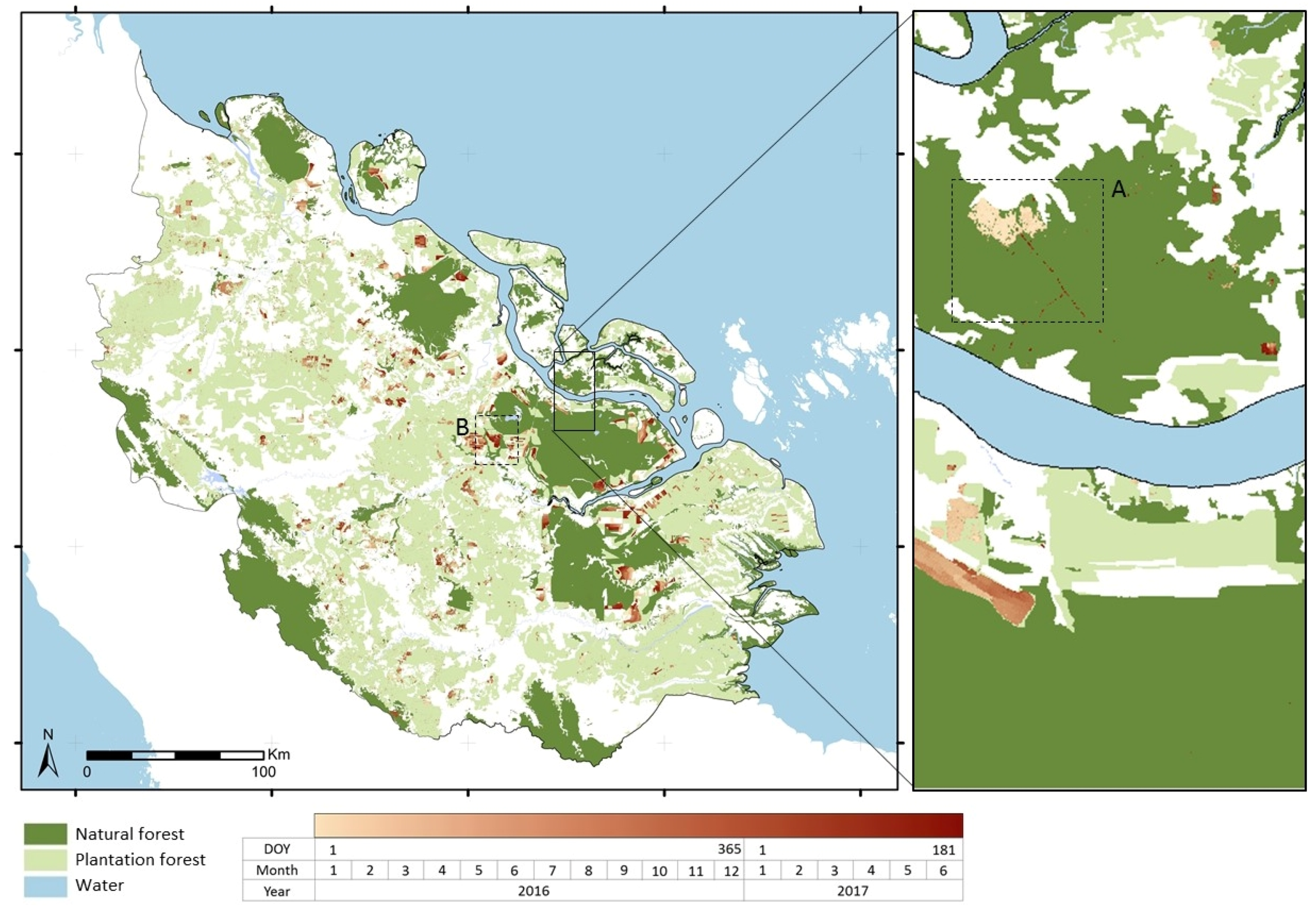
The province of Riau (Figure 1) is located in central Sumatra, Indonesia (centered at 1°N, 102°E), and covers about 9 million ha with elevations up to 1200 m. About 6.4 million people live in Riau. Riau experiences tropical equatorial climate with persistent cloud cover throughout the entire year. Annual precipitation is 2000–3000 mm. The dry season commonly ranges from April to November [5]. Primary and secondary dryland and swamp and mangrove forest dominate the natural forest. Riau has the highest forest-cover-loss rates in Indonesia [1] mainly driven by expansion and conversion to oil palm, acacia, coconut, and rubber plantations [34]. Although forbidden by law, fire use for forest removal is still wide-spread in Riau [5,10]. Figure 1 depicts the 2015 forest land cover map of Indonesia’s Ministry of Environment and Forestry [35] that we used as forest benchmark map for this study. In 2015, remaining natural forest covered ~1.67 million ha (18.5% of Riau’s land area), while plantation forest covered ~3.58 million ha (41.8%). A detailed description on the method used to generate the forest land cover map and a class description can be found in [35]. We follow Indonesia’s forest definition [35] and consider areas with less than 0.25 ha and less than 30% canopy cover as non-forest.
3. Data and Methods
3.1. Sentinel-1 Synthetic Aperture Radar Dataset
Sentinel-1A and -1B C-band SAR images in Interferometric Wide Swath mode (IW, 250 km swath width) were acquired for the period between 1 October 2014 and 30 June 2017 from the Copernicus Open Access Hub [28,29]. In total, 1050 dual-polarized (VV and VH) images were retrieved in ascending (tracks 69 and 171) and descending (tracks 18, 91 and 164) mode provided in Level-1 Ground Range Detected (GRD) format. Starting from 2016, at least 12 daily acquisitions were available (~3.3 observations/month) for most areas, while for earlier periods, fewer observations were available (~2.4 observations/month). We applied automated Sentinel-1 time series processing, including individual image pre-processing and geocoding, quality control, mosaicking, and multi-temporal filtering. Individual image pre-processing using ESA’s (European Space Agency) Sentinel Application Platform (SNAP) toolbox [36] consisted of data import and format conversion, multi-looking (2 × 2 pixel), radiometric calibration (gamma-naught), topographic normalization [37] and geocoding to 20 m pixel resolution (WGS84, Latitude/longitude). Geocoding was done automatically, using ESA Precise Orbits with an estimated absolute geolocation accuracy of below 5 m [38]. The output was geocoded and topographically normalized gamma-naught backscatter images at 20 m resolution. We removed corrupted images and images with geometric artifacts. We applied adaptive multi-temporal SAR filtering [39] to reduce SAR speckle in the data. Finally, we mosaicked all backscatter images acquired at the same date individually for VV and VH polarization.
3.2. Sentinel-1-Based, Near Real-Time Forest Cover Loss Detection
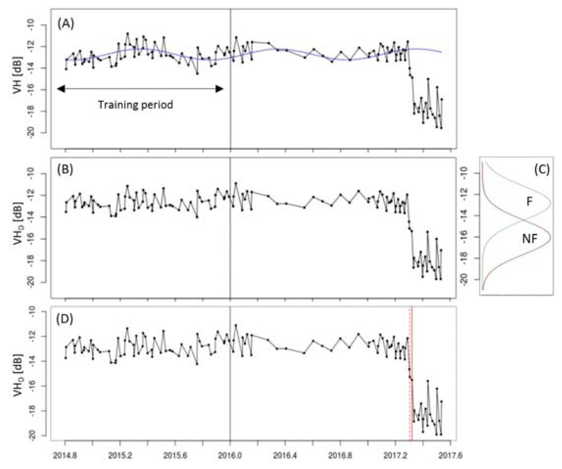
To detect forest-cover loss in near real-time in dense Sentinel-1 time series, we applied a pixel-based time series method on each of the pixels included in the benchmark forest mask. We used the period between 1 October 2014 and 31 December 2015 as training period and the period between 1 January 2016 and 30 June 2017 as monitoring period to detect new forest-cover loss. Figure 2 illustrates the main steps of the method for a single pixel VH backscatter time series covering a dry forest area with a forest-cover-loss event in April 2017. Based on observations during the training period, we first fitted a harmonic model to account for the forest seasonality in the time series (Figure 2A). The harmonic model was subsequently used to remove the forest seasonality (Figure 2B) (Section 3.2.1). Next, the deseasonalized observation in the training period were used to derived pixel specific forest (F) and non-forest (NF) distributions in a data-driven manner (Figure 2C) (Section 3.2.2). The F and NF distributions were used to parameterize a probabilistic approach [40] that was used to detected forest cover loss in near real-time during the monitoring period (Figure 2D) (Section 3.2.3). Finally, we assessed the spatial and temporal accuracy of the method separately for natural forest and plantation forest, and compared the results for VV and VH (Section 3.2.4).
3.2.1. Removing Forest Seasonality Using Harmonic Model Fitting
We fitted a first order harmonic model [41] to the observations in the defined training period using Ordinary Least Squares (OLS) fitting:
with the dependent variable at time t being expressed by the sum of the intercept α, a first-order harmonic component representing seasonality and the residual term εt. γ and δ are the amplitude and phase of the harmonic component. f is the frequency of the time-series. We adapted the initial model of Verbesselt et al. [41] following modifications proposed by DeVries et al. [22]. We fitted a simple first-order harmonic model instead of a multi-order harmonic-trend model to account for forest seasonality while avoiding overfitting, considering the short training period of less than two years. Additionally, the trend component was removed to avoid predicting a possible forest regrowth trend into the monitoring period, which would lead to unrealistic high values [22]. Figure 2A shows the example time series and the fitted first-order harmonic model in blue.
Next, time series observations from the training period and new observations in the monitoring period were deseasonalized by removing the seasonal component estimated in Equation (1):
with being the deseasonalized observation at time t. The deseasonalized VV and VH time series observations are hereafter denoted as VVD and VHD. Figure 2B shows the deseasonalized VHD time series observations for the single pixel example.
3.2.2. Deriving Forest and Non-Forest Distributions
Here, we use a pixel-based and data-driven approach to derive the F and NF distributions from the deseasonalized observations. We assumed all observations during the training period to represent stable F and did not consider possible change and regrowth processes. We calculated the median () and standard deviation (σ) of the F observations during the training period and used them to define the F and NF distributions. We used the median of the F observations during the training period instead of the mean as it is more robust against outliers. We assumed a Gaussian distribution of F and NF based on findings of previous studies for a variety of tropical evergreen and dry forest conditions and for different optical and SAR sensors, including Sentinel-1 [33,40,42]. We defined the F distribution as N(,), with and defining the expectation (mean, median and mode) and the standard deviation of the Gaussian distribution (N). We defined the NF distribution as N(,); with the expectation of NF being below the expectation of the F distribution. This is based on tests done in Sumatra, and confirmed results obtained for Sentinel-1 at a different test site in Bolivia [33]. Deriving F and NF distributions using the proposed pixel-based and data-driven approach considers the pixel-specific variability of the F backscatter signal, a major advantage over approaches that use F and NF training data representing the entire study area [33,40]. In this way, forest pixels with a relatively large variability of the forest signal result in F and NF distributions that are further distant. This reduces unwanted false detections as a result of the high variability of the forest signal. Figure 2C shows the derived F and NF distributions for the single pixel example. The derived F and NF distributions were used as parameterization of the probabilistic approach in the next step.
3.2.3. Probabilistic Approach for Near Real-Time Forest Cover Loss Detection
To detect forest-cover loss in near real-time in the deseasonalized backscatter time series, we used the probabilistic approach proposed in Reiche et al. [40], and available as open-source “bayts” package for R [43]. A brief description is provided here since the probabilistic approach is described in detail in Reiche et al. [40]. We considered a near real-time scenario with past (t-1), current (t) and future observations (t + 1) where individual observations were added chronologically to the time series from the start of the monitoring period onwards (1 January 2016). First, each newly available observation (t = current) was converted to the conditional NF probability using the specific F and NF distributions following Bayes’ theorem. The derived conditional NF probability was added to the time series of conditional NF probabilities derived from the previous observations (t–i). Second, we flagged a potential forest cover loss event in the case that the conditional NF probability was larger than 0.5. We calculated the probability of forest-cover loss using iterative Bayesian updating. Future observations (t + i) were used to update the probability of forest cover loss in order to confirm or reject the flagged forest-cover-loss event. Forest-cover-loss events were confirmed if the conditional probability of forest-cover loss exceeded a defined threshold χ. The χ threshold value can range between 0 and <1 with higher χ threshold values increasing the confidence of confirmed forest-cover-loss events. In case the conditional probability of forest-cover loss decreased below 0.5, we considered it to be falsely indicated, unflagged the event, and continued monitoring [40]. Figure 2D shows the detected forest cover loss for the example VH time series. The time of flagged (red dotted line) and confirmed changes (red line) are shown.
3.2.4. Assessing the Spatial and Temporal Accuracy
We validated the proposed method for Sentinel-1-based forest-cover loss detection with respect to its near real-time performance. We analyzed the results for increasing χ threshold values from χ = 0.5 to χ = 0.975 in steps of 0.025, separately for VV and VH. We used land cover information from Indonesia’s Ministry of Environment and Forestry (Figure 1; [35]) to assess the forest-cover loss separately for natural and plantation forest. We followed Indonesia’s forest definition and removed isolated areas smaller 0.25 ha.
We estimated the spatial and temporal accuracy for the forest-cover loss maps, separately for natural and plantation forest. In the absence of suitable reference data, we followed Olofsson et al. [44] and generated an initial forest-cover loss map using a high χ threshold value of 0.9. Forest-cover loss was 0.83% (13 833 ha) of the natural forest area, and 7.91% (282,921 ha) of plantation forest area. Separately for natural forest and plantation forest, we generated 600 sample points using probability sampling [45]. We allocated 100 sample points to the change stratum (forest cover loss) to account for the small area proportion and to ensure a reliable estimation of the producer’s and user’s accuracy of the class. The remaining 500 points were allocated to the no-change stratum (stable forest cover). We checked each of the sample points for showing forest-cover loss during the monitoring period by systematically tracing the images of the VV and VH time series (Figure 3). This was supported by visual interpretation using high spatial resolution imagery available in Google Earth and the Planet Labs data archive [46]. Misclassified samples were assigned to the correct class. For the change pixels, we also documented the date at which the forest-cover loss was visible for the first time (tref). The approach is consistent with approaches used in previous studies [21,22,33,47,48].
We calculated the area-adjusted overall accuracy (OA), producer’s accuracy (PA; 1—omission error), and user’s accuracy (UA; 1—commission error) following Olofsson et al. [44]. We treated detected forest-cover-loss events that have been flagged earlier than first visible in the time series as commission errors. Due to the very small area proportion of the change class, the OA is mainly driven by the UA and PA of the dominating no-change stratum and is not a good measure to assess the method performance to detect forest-cover loss. The UA and PA of the change stratum is a more useful measure.
To estimate the temporal accuracy, we followed Reiche et al. [33] and calculated the adjusted mean time lag of confirmed forest cover loss events (MTL), and the adjusted mean time lag of the time at which the confirmed forest cover loss events were initially flagged (MTLF). By calculating the adjusted mean time lag, we reduced the imprecision of the reference date. While the date at which forest cover loss was first visible in the time series (Tref) is commonly considered as reference date, it does not represent the true date of change. The true date of change instead occurred sometime in between Tref and the previous time step (Tref_previous). We therefore calculated the adjusted reference time (Tref_adjusted) to be right in between Tref and Tref_previous [33]. Figure 2 illustrates a sample validation pixel showing forest-cover loss between 2017 (136) (tref_previous) and 2017 (147) (tref). For the validation pixel, Tref_adjusted was 2017 (141.5). For the entire reference dataset, the mean time difference between Tref and Tref_preveeous was 11.9 ± 1.5 days (95%) at natural forest and 9.5 ± 1.3 days (95%) at plantation forest. Using Tref_adjusted as a reference to calculate the time lag reduced the bias of the reference date to 5.95 ± 0.75 days (95%) and 4.75 ± 0.63 days (95%), for natural and plantation forest, respectively.
3.3. Characterizing Fire-Related Forest-Cover Loss Using Active Fire Alerts
We used VIIRS active fire alerts (V14IMGTDL_NRT, [18]) to (i) determine the fraction of fire-related forest-cover loss and (ii) compare the timing of active fires and forest-cover loss, and separate active fires that predate, coincide with, and postdate forest-cover loss. VIIRS provides active fire alerts every 12 h at 375 m resolution [18]. All VIIRS active fire alerts available for the monitoring period and six months before and after (1 July 2015 and 31 December 2017) were downloaded from the Fire Management and Resource Management System (FIRMS). Including alerts from six months before and after the monitoring period considers fires that predate or postdate the forest cover loss events detected at the beginning and end of the monitoring period. In total, 3080 alerts were available for natural forest and 10,979 were available for plantation forest.
We identified fire-related forest cover loss by co-locating clumped forest cover loss pixels with active fire alerts. This approach is consistent with approaches used in previous studies combining active fire alerts with remote-sensing-based forest-change products [5,10,16,19]. We used the 2015 forest land cover (Figure 1; [35]) of Indonesia’s Ministry of Environment and Forestry to separate fire-related changes for different natural forest classes.
We compared the timing of active fire alerts and forest-cover-loss events. First, we calculated the median detection date of all 20 m Sentinel-1 pixels detected as forest-cover loss within a 375 m VIIRS pixel. We used the date at which forest-cover-loss events were first flagged. Secondly, we corrected the median detection date by subtracting the calculated MTLF. The corrected median detection date represents a more realistic estimate of the true date of forest-cover loss. Thirdly, we calculated the time difference of the VIIRS active fire alert and the corrected median detection date. Next, we separate active fires that predate, coincide with, or postdate forest-cover loss. Next, we added the remaining uncertainty of the reference data (natural forest: 5.95 ± 0.75 days (95%): plantation forest: 4.75 ± 0.63 days (95%)), and the uncertainty of the MTLF (natural forest: 7.5 ± 3.8 days (95%); plantation forest 7.2 ± 2.4 days (95%); taken from results in Section 4.1). Fire alerts with a time difference in the range of the added uncertainty were considered to coincide with forest cover loss. Fire alerts with a time difference exceeding the added uncertainty were considered as fires predating or postdating forest-cover loss.
4. Results
4.1. Sentinel-1-Based, Near Real-Time Forest Cover Loss Detection
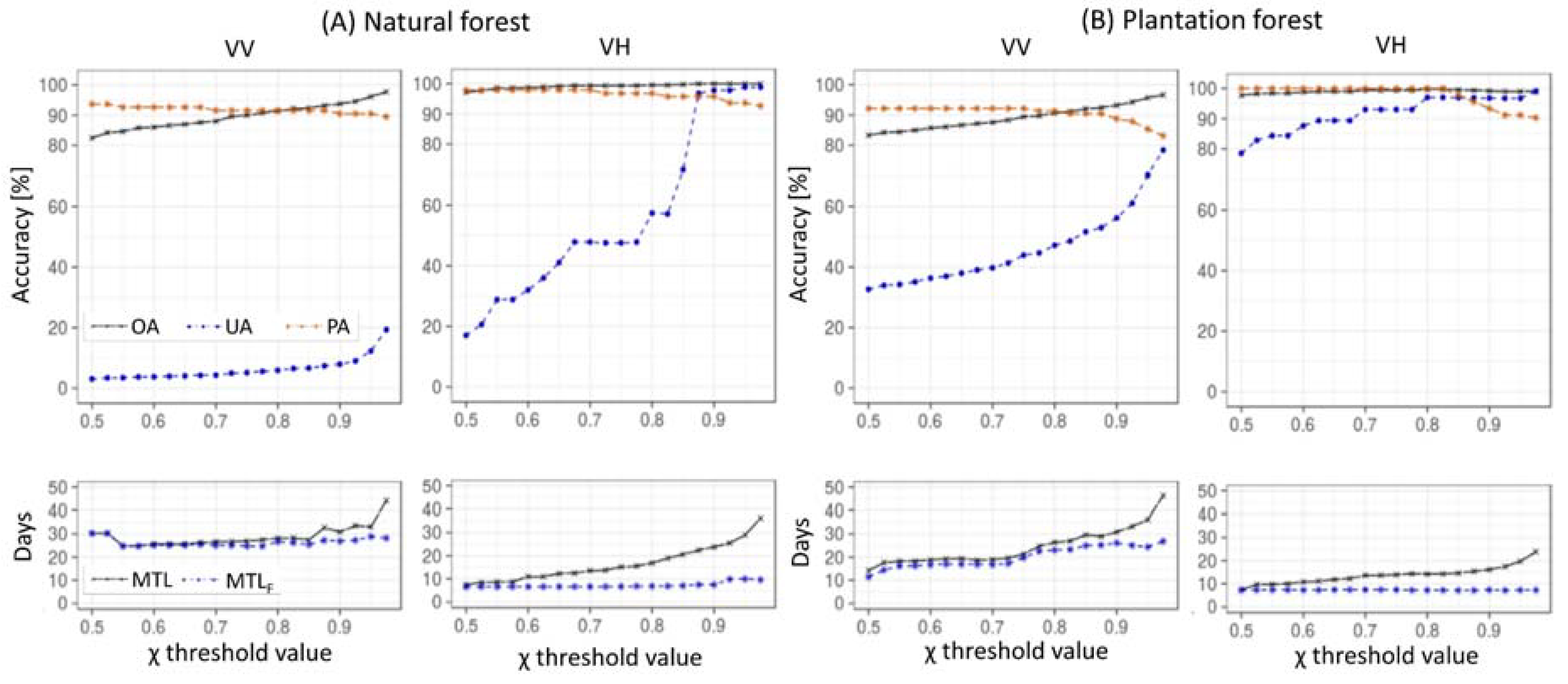
The spatial accuracy (OA; PA and UA of the forest-cover-loss class) and temporal accuracy (MTL and MTLF) for Sentinel-1-based, near real-time forest-cover-loss detection using VV and VH are shown in Figure 4 for increasing χ threshold values, separately for natural and plantation forest. The results can be summarized as follows. For all scenarios, we found increasing UA and PA of the change class (forest-cover loss) for increasing χ threshold values. The UA and PA for the no-change class (not shown in Figure 4) were generally higher than the UA and PA for the change class. The MTL increased with increasing χ threshold values while the MTLF was similar for all χ threshold values.
For both natural and plantation forest, the spatial and temporal accuracies found for VV were consistently lower when compared to VH. Results for VH in natural forest (Figure 4A) showed a UA/PA cross-over point at χ = 0.875 with a UA of 96.8% and a PA of 95.8%. The MTL was found to be 22.4 ± 3.9 days (95%) and the MTLF was 7.5 ± 3.8 days (95%). The highest UA was achieved for χ = 0.975 and was 98.8%. For χ = 0.975, the PA was 92.7% and the MTL was 36.2 ± 4.8 days (95%). Results for VH in plantation forest (Figure 4B) showed higher UA’s and lower MTL’s. As for natural forest, the UA/PA cross-over point was found at χ = 0.875 with a UA of 96.9% and a PA of 95.6%. The MTL was 15.4 ± 2.8 days (95%) and the MTLF was 7.2 ± 2.4 days (95%).
We generated a final forest-cover loss map using a χ threshold value of 0.875 for VH (Figure 5). This corresponds to the UA/PA cross-over point for both natural and plantation forest with both UA and PA above 95%. This allows for high confident forest-cover-loss detection, which is important for a robust comparison with active fire alerts. Figure 6 provides detailed maps showing encroachment into natural forest (Figure 6A), and large-scale plantation dynamics (Figure 6B).
4.2. Fire-Related Forest Cover Loss
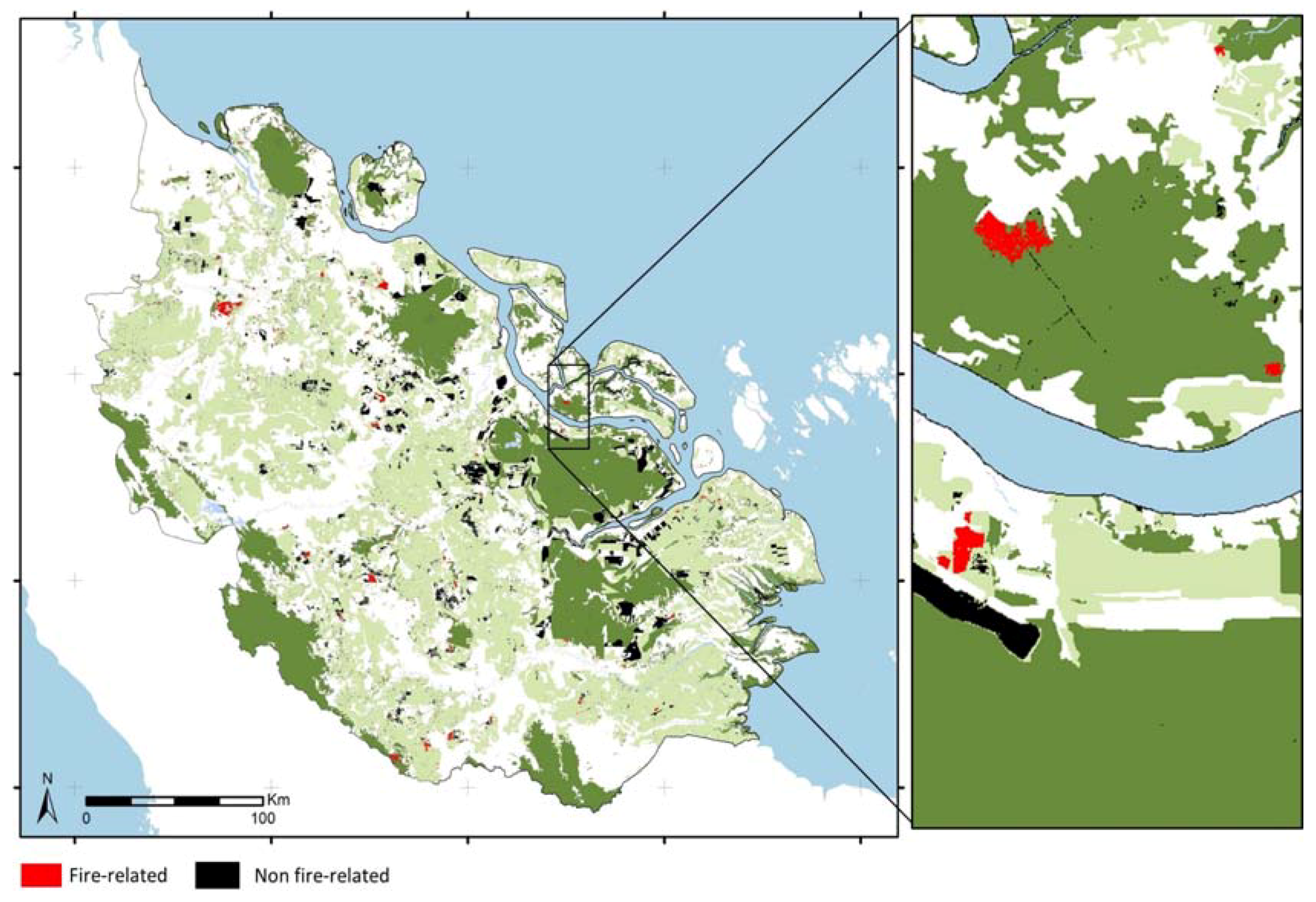
Figure 7 depicts fire-related versus non-fire-related forest-cover loss for the study area. For the 18-month monitoring period, natural forest-cover loss accounted for 14,372 ha (0.86% of the natural forest area), of which 33.6% (4823 ha) was fire-related. The large majority of the fire-related natural forest-cover loss was detected over secondary forest (4757 ha of 14,022 ha), and only a small percentage over primary forest (66 ha of 350 ha). Comparing the major natural forest-cover types showed that fire-related forest-cover loss in dryland, swamp, and mangrove forest was 1937 ha, 2835 ha, and 41 ha, respectively. The mean size of natural forest-cover-loss pixel clusters was 2.2 ha. Plantation forest-cover loss accounted for 295,205 ha (~8.2% of the plantation area), of which 8.4% (24,792 ha) was fire-related. The mean size of forest-cover-loss pixel clusters in plantations was 8.1 ha.
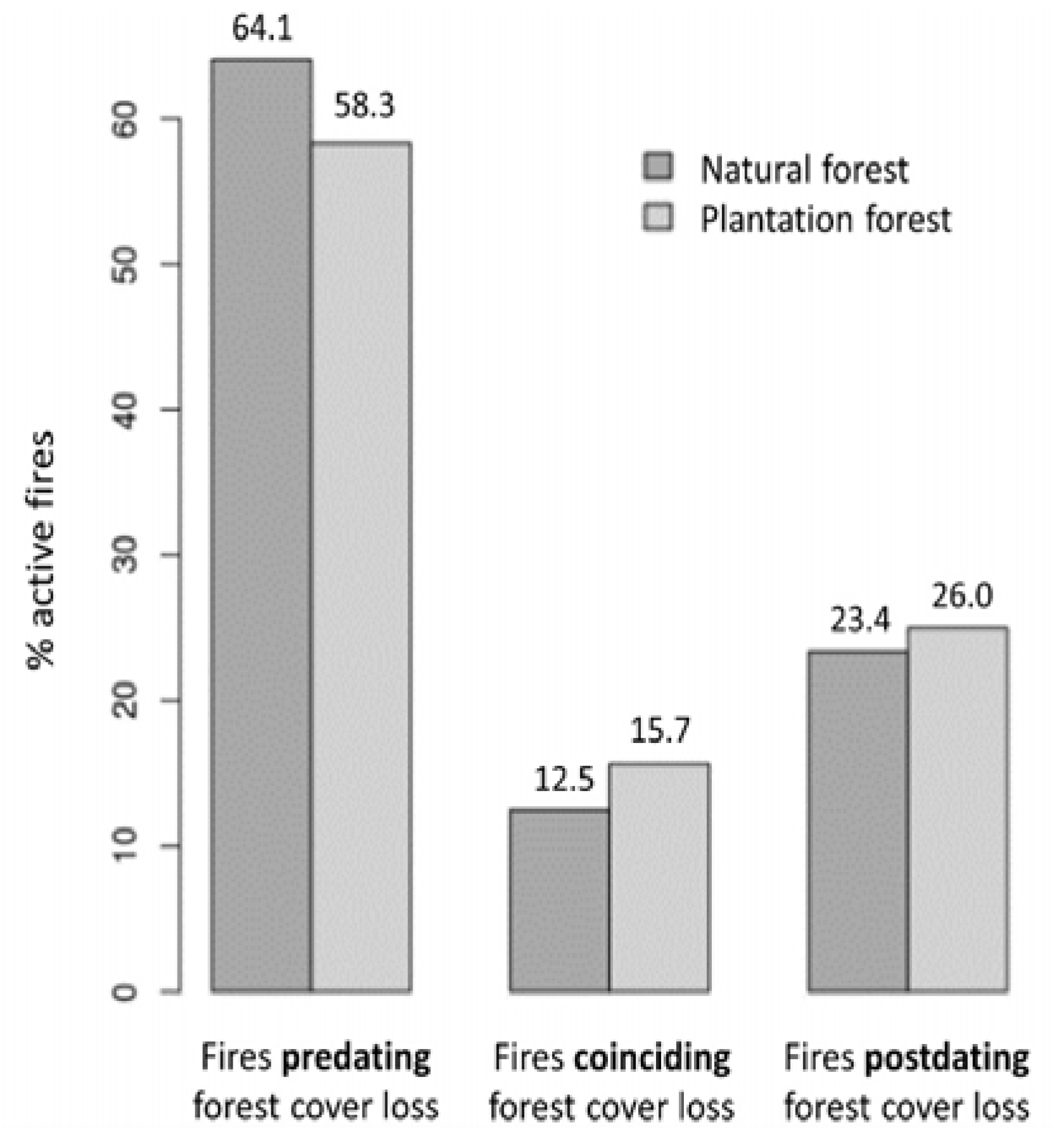
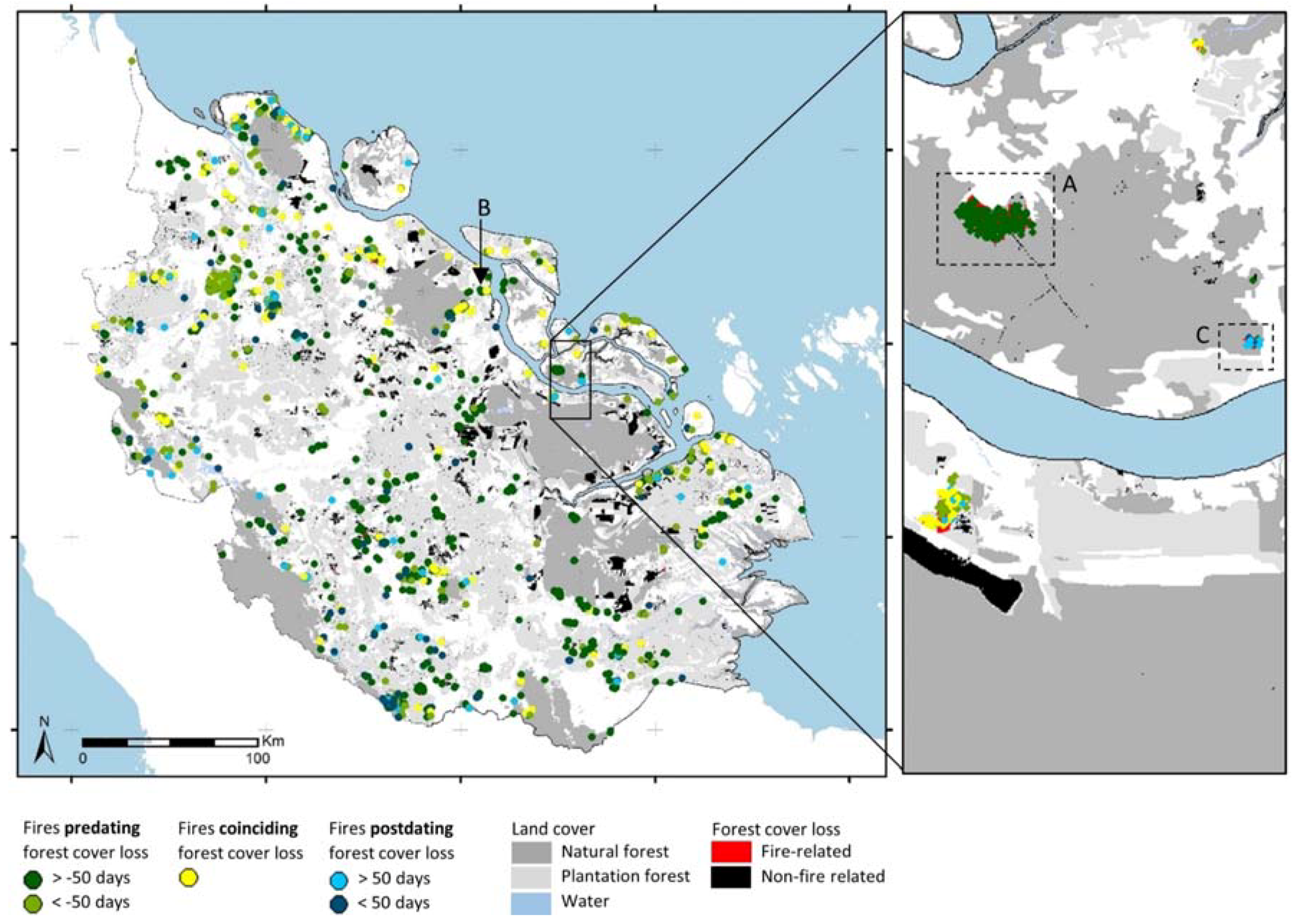
Figure 8 shows percentages of active fires predating, coinciding with, and postdating forest cover loss. In natural forest, active fires that predated, coincided with, and postdated forest cover loss accounted for 64.1%, 12.5%, and 23.4% of the total forest-cover-loss-related fires. In plantation forest, active fires that predated, coincided with and postdated forest-cover loss accounted for 58.3%, 15.7% and 26% of the total forest-cover-loss-related fires. Active fires were found to occur an average of 57.9 ± 10.3 days (95%) and 67.4 ± 6.3 days (95%) before forest-cover loss in natural and plantation forest, respectively. Active fire alerts were found to occur up to more than 200 days before and after the forest-cover loss events. Figure 9 depicts the spatial pattern of fires predating, coinciding with and postdating forest-cover loss. Figure 10 shows three detailed maps with fire (Figure 10A) predating, (Figure 10B) coinciding with, and (Figure 10C) postdating forest-cover loss; supported by high-resolution satellite imagery and pixel time series examples.
5. Discussion
In this study, we combined temporally dense Sentinel-1-based forest-cover loss information with active fire alerts to characterize tropical forest-cover loss in the Province of Riau, Indonesia. For the 18-month period between 1 January 2016 and 30 June 2017, we detected 14,372 ha of natural forest-cover loss, of which 33.6% (4823 ha) was fire-related. We detected 2835 ha of fire-related forest cover loss over highly threatened swamp forest, which can be linked to large greenhouse gas emissions [5,49]. About 64% of the fires in natural forest predated forest-cover loss, about 13% coincided with forest-cover loss, and 23% postdated forest-cover loss. In plantation forest, we detected 256,349 ha of forest-cover loss due to mainly plantation dynamics, of which 8.4% (24,792 ha) was fire-related. The low percentage of fire-related forest cover loss in plantation forest confirms the decreasing trend found by Noojipady et al. [10] being linked to effective implementation of certification schemes for fire-free plantation management [50]. About 58% of the fires in plantation forest predated forest-cover loss, about 16% coincided with forest-cover loss, and 26% postdated forest-cover loss.
5.1. Sentinel-1-Based, Near Real-Time Forest Cover Loss Detection
Results demonstrate the potential of dense Sentinel-1 C-band SAR data with guaranteed observations of at least every 12 days to provide confident, timely and gap-free forest-cover loss information in a heterogeneous tropical forest environment with varying change dynamics and scales. Here, we applied a pixel-based time series method to detect forest-cover loss in near real-time in Sentinel-1 time series. We first used harmonic model-fitting [22,51] to account for forest seasonality, and subsequently used a probabilistic approach [40] to detect forest-cover loss in near real-time. Using pixel-based harmonic model fitting [51] enabled to account for forest seasonality in Riau varying from no (swamp forest) (Figure 6A) to stronger forest seasonality (dryland forest) (Figure 2), confirming results of many other studies [22,51,52]. While in previous studies at small test sites [33,40], training data for forest and non-forest was used to represent the entire study area to parameterize the probabilistic approach, here we proposed a pixel-based and data-driven approach to derive the forest and non-forest distributions. This enabled the application of the probabilistic approach to a larger area with heterogeneous forest types. A limitation of the pixel-based approaches is the relatively low number of observations during the training period (~40 to 70) used to derive the forest distributions. With Sentinel-1 continuously acquiring data, an increasing number of training observations will be available for future studies, improving the robustness of the proposed pixel-based approach.
While forest-cover loss was detected with UA’s and PA’s above 95% (χ = 0.875) for both natural and plantation forest, it required an average of 7 days longer to confirm forest-cover loss in natural forest (MTL = 22 days) when compared to plantation forest (MTL = 15 days). This can primarily be related to different change processes and dynamics in natural and plantation forest. Plantation forest was characterized by large-scale loss of forest cover in monocultures (average patch size = 8.1 ha) with all trees and understory being removed entirely to prepare the plantation concessions for new cultivation (Figure 6B). This leads to large forest/non-forest contrast in the C-band SAR signal, requiring few observations to confirm a forest-cover loss event with high confidence. In contrast, forest-cover loss in natural forest was often small-scale (average patch size = 2.2 ha) with more subtle changes (Figure 6A). After forest logging, understory vegetation often remains, causing a more subtle forest/non-forest contrast in the C-band signal as C-band interacts in a similar way with forest canopy and understory vegetation [53]. More observations were required to confirm forest-cover loss with high confidence. Results showed that forest-cover loss was detected with more timeliness and more accuracy for VH when compared to VV, reflecting the higher sensitivity of cross-polarized VH to detect forest change when compared to single-polarized VV [54,55]. Results for plantation forest obtained for VV are very similar to the results found for large-scale harvesting dynamics in Bolivia [33].
Our results confirm the clear trade-off between spatial and temporal accuracy which are inherent for time-series-based, near real-time forest-monitoring systems [22,33,52,56]. While we used a χ threshold values of 0.875 (UA/PA cross-over) to detect forest-cover loss with high confidence in order to allow a robust integration with active fire alerts, different use case scenarios may be considered. A lower χ threshold value, for example, results in forest-cover loss events being confirmed in a timelier manner, but at the costs of increased false detections. Using a χ threshold values of 0.725 results in forest-cover loss being confirmed over natural forest within 14 days (MTL = 13.8 days), but it is associated with a lower PA of 47.9%. This shows the flexibility of our approach to adjust for different user needs. Ultimately, user needs decide upon which scenario to choose [33].
We corrected the forest-cover loss detection dates using the calculated adjusted mean time lag [33]. This resulted in a robust estimation of the true date of forest-cover loss, and in turn, a valid comparison of the timing with VIIRS active fire alerts. Having detailed information on the remaining uncertainty of the mean time lag of detected changes and the reference date derived from the dense and regular Sentinel-1 time series enabled us to identify fires that significantly predated and postdated forest-cover loss.
5.2. Characterizing Fire-Related Forest-Cover Loss
For the first time, the temporal relation between active fires and tropical forest-cover loss was analyzed at high temporal detail. In contrast to studies relating active fire alerts with annual forest change and thus are limited to quantifying fire-related forest change [5,10,16,19,20], here we were able to separate fires that predate, coincide with, and postdate forest-cover loss. Clear spatial-temporal patterns were found with entire patches where active fires either predated, coincided with, or postdated forest cover loss (Figure 9 and Figure 10).
The minority of fires in natural and plantation forest temporally coincided with forest-cover loss (13% and 16%) and can thus be confidently attributed as a direct cause of the forest-cover loss. Fire use for forest removal is a common management practice by plantation operators and smallholder farmers [13,57]. For smallholders, fire use is the most cost–efficient way to remove forest and expand agricultural land, where machinery which can reduce the costs of logging operations is not available [57,58]. Fires lit by communities which accidently spread to nearby forest areas are also a potential driver of fires coinciding with forest-cover loss [13]. Fires predating forest-cover loss can often be attributed to pre-logging fires used to remove the forest understory in order to make it more accessible for later logging operations [59]. Also, logging operations after natural fires that did not lead to the actual removal of the forest canopy may contribute. Fires postdating forest-cover loss can often be attributed to post-harvest burning in order to remove the remaining vegetation and prepare the land for new cultivation [5,13]. However, it is still unclear if only remaining vegetation is burned and the timber removed or whether the timber is piled up and burned [12]. While it is possible to attribute potential reasons for human-induced fires which predate, coincide with, and postdate forest-cover loss, it’s difficult to separate human-induced fires from natural fires. However, only the minority of fires in Indonesia are natural [5,8].
Results for both natural forest and plantation forest suggest that active fires occurred an average of around 58 and 67 days before forest-cover loss, with some active fires occurring more than 200 days before and after forest-cover loss events. While fires temporally close to forest-cover loss can be related with high certainty, it is unclear how long before and after the event that fires are likely to still be related to forest-cover loss. Studies showed that fire may continue up to 1–3 years after forest removal to complete the burning of remaining vegetation [12]; however, it is unlikely that fires occurring 1–3 years before the forest-cover-loss event are related in a similar manner. In summary, to attribute key fire-management practices in a robust manner to forest-cover-loss events requires further insights and assumptions.
Combining 375 m VIIRS active fire alerts with forest-cover loss alerts at 20 m spatial resolution can be used to identify small-scale fire-related forest-cover loss. Further studying the spatial-temporal pattern of fire-related forest-cover loss may allow locating individual ignition sources that, for example, give rise to uncontrolled fires during drought periods [14].
Optical and SAR sensor difference should be considered when linking active fire data with remote sensing-based forest-cover loss information. While C-band SAR only detect the effect of fires where the forest canopy is, to a large extent, removed [60,61], optical sensors can detect the effect of crown fires through burned canopy foliage. Using optical data, however, does not allow a straightforward separation of fires which result in only burned canopy foliage and those which result in actual forest-cover loss [62]. This, however, has a large effect on the greenhouse gas emissions. A combination of active fire alerts with dense Sentinel-1 and optical Sentinel-2 data may allow a further characterization and attribution of fire-related change processes in tropical forest, towards improved estimates of greenhouse gas emissions from fire.
6. Conclusions
This study combines temporally dense Sentinel-1 data and active fire alerts to characterize fire-related tropical forest-cover loss. We first evaluated Sentinel-1-based, near real-time forest-cover-loss detection in natural and plantation forest. Next, we combined the Sentinel-1-based forest-cover-loss information with active fire alerts, and separated active fires that predate, coincide with and postdate forest-cover loss. Results for the Province of Riau, Indonesia show that dense Sentinel-1 C-band SAR time series provide confident, timely, and gap-free forest-cover-loss detection in both natural and plantation forest. Having such dense and regular information on forest-cover loss available enabled an assessment of the temporal relation between active fires and tropical forest-cover loss at high temporal detail. Fire-related forest-cover loss accounted for about one third of the natural forest-cover loss, while in plantation forest, less than ten percent of the forest-cover loss was fire-related. Clear spatial patterns of fires predating, coinciding with, or postdating forest-cover loss patches were found. We discussed the attribution of management practices. Only the minority of fires in natural and plantation forest temporally coincided with forest-cover loss and can thus be confidently attributed as the direct cause of forest-cover loss. The majority of the fires predated or postdated forest-cover loss and should be attributed to other key management practices. While this paper addressed some of the questions on how fire and forest-cover loss are temporally related, further research is needed for a robust characterization of fire-related forest-cover loss towards a more accurate estimation of greenhouse gas emissions from fires. The work presented in this study may lead the way forward to a fully-integrated near real-time system linking active fire alerts with Sentinel-1-based forest-cover-loss information. Such systems can support stakeholders, companies and watchdog organizations for more effective and timely law enforcement to reduce the illegal and unsustainable use of fires in tropical natural and plantation forest.
Author Contributions
All authors conceived and designed the experiments; J.R. and R.V. processed the data. J.R. carried out the method development, performed the experiments, and wrote the paper.
Funding
This research was partly funded by the European Commission Horizon 2020 BACI project [grant number 640176] and the European Commission Horizon 2020 openEO project [grant number 776242].
Acknowledgments
The work of J.R. and M.H. was funded by the European Commission Horizon 2020 BACI project (grant number 640176) and European Commission Horizon 2020 openEO project (grant agreement 776242). The work of E.H. was funded by the Center for International Forestry Research (CIFOR). The work of J.V. was funded by the European Commission 2020 openEO project (grant number 776242). This work was supported by the Global Forest Observation Initiative (GFOI) research and development program. This work contains modified Copernicus Sentinel-1 data (2014–2017). We acknowledge the use of data and imagery from LANCE FIRMS operated by the NASA/GSFC/Earth Science Data and Information System (ESDIS) with funding provided by NASA/HQ. Planet data was provided through the Planet ambassador program. We acknowledge Frank-Martin Seifert from ESA for his support, and Fred Stolle from World Resource Institute (WRI) for his valuable input. Thanks to Sarah Carter from Wageningen University for proof-reading the manuscript.
Conflicts of Interest
The authors declare no conflict of interest.
References
- Margono, B.A.; Potapov, P.V.; Turubanova, S.; Stolle, F.; Hansen, M.C. Primary forest cover loss in Indonesia over 2000–2012. Nat. Clim. Chang. 2014, 4, 730–735. [Google Scholar] [CrossRef]
- Hansen, M.C.; Potapov, P.V.; Moore, R.; Hancher, M.; Turubanova, S.A.; Tyukavina, A.; Thau, D.; Stehman, S.V.; Goetz, S.J.; Loveland, T.R.; et al. High-resolution global maps of 21st-century forest cover change. Science 2013, 342, 850–853. [Google Scholar] [CrossRef] [PubMed]
- Tsujino, R.; Yumoto, T.; Kitamura, S.; Djamaluddin, I.; Darnaedi, D. History of forest loss and degradation in Indonesia. Land use policy 2016, 57, 335–347. [Google Scholar] [CrossRef]
- Harrison, M.E.; Page, S.E.; Limin, S.H. The global impact of Indonesian forest fires. Biologist 2009, 56, 156–163. [Google Scholar]
- Gaveau, D.L.A.; Salim, M.A.; Hergoualc’H, K.; Locatelli, B.; Sloan, S.; Wooster, M.; Marlier, M.E.; Molidena, E.; Yaen, H.; DeFries, R.; et al. Major atmospheric emissions from peat fires in Southeast Asia during non-drought years: Evidence from the 2013 Sumatran fires. Sci. Rep. 2014, 4, 1–7. [Google Scholar] [CrossRef] [PubMed] [Green Version]
- Roy, D.P.; Wulder, M.A.; Loveland, T.R.; Woodcock, C.E.; Allen, R.G.; Anderson, M.C.; Helder, D.; Irons, J.R.; Johnson, D.M.; Kennedy, R.; et al. Landsat-8: Science and product vision for terrestrial global change research. Remote Sens. Environ. 2014, 145, 154–172. [Google Scholar] [CrossRef]
- Van Der Werf, G.R.; Randerson, J.T.; Giglio, L.; Van Leeuwen, T.T.; Chen, Y.; Rogers, B.M.; Mu, M.; Van Marle, M.J.E.; Morton, D.C.; Collatz, G.J.; et al. Global fire emissions estimates during 1997–2016. Earth Syst. Sci. Data 2017, 9, 697–720. [Google Scholar] [CrossRef]
- Qadri, S.T. Fire, smoke, and Haze: The ASEAN Response Strategy; 2001; Volume 10, ISBN 971-561-338-1. [Google Scholar]
- Cattau, M.E.; Harrison, M.E.; Shinyo, I.; Tungau, S.; Uriarte, M.; DeFries, R. Sources of anthropogenic fire ignitions on the peat-swamp landscape in Kalimantan, Indonesia. Glob. Environ. Chang. 2016, 39, 205–219. [Google Scholar] [CrossRef]
- Noojipady, P.; Morton, D.C.; Schroeder, W.; Carlson, K.M.; Huang, C.; Gibbs, H.K.; Burns, D.; Walker, N.F.; Prince, S.D. Managing fire risk during drought: The influence of certification and El Ninõ on fire-driven forest conversion for oil palm in Southeast Asia. Earth Syst. Dyn. 2017, 8, 749–771. [Google Scholar] [CrossRef]
- Gaveau, D.L.A.; Sloan, S.; Molidena, E.; Yaen, H.; Sheil, D.; Abram, N.K.; Ancrenaz, M.; Nasi, R.; Quinones, M.; Wielaard, N.; et al. Four Decades of Forest Persistence, Clearance and Logging on Borneo. PLoS ONE 2014, 9, e101654. [Google Scholar] [CrossRef] [PubMed] [Green Version]
- Morton, D.C.; Defries, R.S.; Randerson, J.T.; Giglio, L.; Schroeder, W.; van der Werf, G.R. Agricultural intensification increases deforestation fire activity in Amazonia. Glob. Chang. Biol. 2008, 14, 2262–2275. [Google Scholar] [CrossRef]
- Dennis, R.A.; Mayer, J.; Applegate, G.; Chokkalingam, U.; Colfer, C.J.P.; Kurniawan, I.; Lachowski, H.; Maus, P.; Permana, R.P.; Ruchiat, Y.; et al. Fire, people and pixels: Linking social science and remote sensing to understand underlying causes and impacts of fires in Indonesia. Hum. Ecol. 2005, 33, 465–504. [Google Scholar] [CrossRef]
- Carlson, K.M.; Curran, L.M.; Asner, G.P.; Pittman, A.M.; Trigg, S.N.; Marion Adeney, J. Carbon emissions from forest conversion by Kalimantan oil palm plantations. Nat. Clim. Chang. 2012, 3, 283–287. [Google Scholar] [CrossRef]
- Stolle, F.; Chomitz, K.M.; Lambin, E.F.; Tomich, T.P. Land use and vegetation fires in Jambi Province, Sumatra, Indonesia. For. Ecol. Manag. 2003, 179, 277–292. [Google Scholar] [CrossRef]
- Miettinen, J.; Shi, C.; Liew, S.C. Fire Distribution in Peninsular Malaysia, Sumatra and Borneo in 2015 with Special Emphasis on Peatland Fires. Environ. Manag. 2017, 60, 747–757. [Google Scholar] [CrossRef] [PubMed]
- Giglio, L.; Schroeder, W.; Justice, C.O. The collection 6 MODIS active fire detection algorithm and fire products. Remote Sens. Environ. 2016, 178, 31–41. [Google Scholar] [CrossRef]
- Schroeder, W.; Oliva, P.; Giglio, L.; Csiszar, I.A. The New VIIRS 375m active fire detection data product: Algorithm description and initial assessment. Remote Sens. Environ. 2014, 143, 85–96. [Google Scholar] [CrossRef]
- Lohberger, S.; Stängel, M.; Atwood, E.C.; Siegert, F. Spatial evaluation of Indonesia’s 2015 fire-affected area and estimated carbon emissions using Sentinel-1. Glob. Chang. Biol. 2017, 1–11. [Google Scholar] [CrossRef] [PubMed]
- Schroeder, T.A.; Wulder, M.A.; Healey, S.P.; Moisen, G.G. Mapping wildfire and clearcut harvest disturbances in boreal forests with Landsat time series data. Remote Sens. Environ. 2011, 115, 1421–1433. [Google Scholar] [CrossRef]
- Hansen, M.C.; Krylov, A.; Tyukavina, A.; Potapov, P.V.; Turubanova, S.; Zutta, B.; Ifo, S.; Margono, B.; Stolle, F.; Moore, R. Humid tropical forest disturbance alerts using Landsat data. Environ. Res. Lett. 2016, 11, 34008. [Google Scholar] [CrossRef]
- DeVries, B.; Verbesselt, J.; Kooistra, L.; Herold, M. Robust monitoring of small-scale forest disturbances in a tropical montane forest using Landsat time series. Remote Sens. Environ. 2015, 161, 107–121. [Google Scholar] [CrossRef]
- Souza, C.M.; Siqueira, J.V.; Sales, M.H.; Fonseca, A.V.; Ribeiro, J.G.; Numata, I.; Cochrane, M.A.; Barber, C.P.; Roberts, D.A.; Barlow, J. Ten-Year Landsat Classification of Deforestation and Forest Degradation in the Brazilian Amazon. Remote Sens. 2013, 5, 5493–5513. [Google Scholar] [CrossRef]
- Hammer, D.; Kraft, R.; Wheeler, D. Alerts of forest disturbance from MODIS imagery. Int. J. Appl. Earth Obs. Geoinform. 2014, 33, 1–9. [Google Scholar] [CrossRef]
- Watanabe, M.; Koyama, C.; Hayashi, M.; Kaneko, Y.; Shimada, M. Development of early-stage deforestation detection algorithm (advanced) with PALSAR-2/ScanSAR for JICA-JAXA program (JJ-FAST). IEEE Int. Geosci. Remote Sens. Symp. 2017, 2446–2449. [Google Scholar] [CrossRef]
- Hansen, M.C.; Loveland, T.R. A review of large area monitoring of land cover change using Landsat data. Remote Sens. Environ. 2012, 122, 66–74. [Google Scholar] [CrossRef]
- Sannier, C.; McRoberts, R.E.; Fichet, L.-V.; Makaga, E.M.K. Using the regression estimator with Landsat data to estimate proportion forest cover and net proportion deforestation in Gabon. Remote Sens. Environ. 2014, 151, 138–148. [Google Scholar] [CrossRef]
- Potin, P.; Rosich, B.; Miranda, N.; Grimont, P. Sentinel-1 Mission Status. Procedia Comput. Sci. 2016, 100, 1297–1304. [Google Scholar] [CrossRef]
- Torres, R.; Snoeij, P.; Geudtner, D.; Bibby, D.; Davidson, M.; Attema, E.; Potin, P.; Rommen, B.; Floury, N.; Brown, M.; et al. GMES Sentinel-1 mission. Remote Sens. Environ. 2012, 120, 9–24. [Google Scholar] [CrossRef]
- ESA. Sentinel High Level Operations Plan (HLOP); ESA: Paris, France, 2017. [Google Scholar]
- Reiche, J.; Lucas, R.; Mitchell, A.L.; Verbesselt, J.; Hoekman, D.H.; Haarpaintner, J.; Kellndorfer, J.M.; Rosenqvist, A.; Lehmann, E.A.; Woodcock, C.E.; et al. Combining satellite data for better tropical forest monitoring. Nat. Clim. Chang. 2016, 6. [Google Scholar] [CrossRef]
- Delgado-Aguilar, M.J.; Fassnacht, F.E.; Peralvo, M.; Gross, C.P.; Schmitt, C.B. Potential of TerraSAR-X and Sentinel 1 images to map deforested areas and derive degradation status in complex rain forests of Ecuador. Int. For. Rev. 2017, 19, 102–118. [Google Scholar] [CrossRef]
- Reiche, J.; Hamunyela, E.; Verbesselt, J.; Hoekman, D.; Herold, M. Improving near-real time deforestation monitoring in tropical dry forests by combining dense Sentinel-1 time series with Landsat and ALOS-2 PALSAR-2. Remote Sens. Environ. 2018, 204, 147–161. [Google Scholar] [CrossRef]
- Uryu, Y.; Mott, C.; Foead, N.; Yulianto, K.; Budiman, A.; Takakai, F.; Purastuti, E.; Fadhli, N.; Jaenicke, J.; Hatano, R.; et al. Deforestation, Forest Degradation, Biodiversity Loss and CO2 Emissions in Riau, Sumatra, Indonesia. WWF Indones. Tech. Rep. 2008, 1–80. [Google Scholar]
- MoEF. National Forest Reference Emission Level For Deforestation and Forest Degradation: In the Context of Decision 1/CP. 16 Para 70 UNFCCC (Encourages Developing Country Parties to Contribute to Mitigation Actions in the Forest Sector); MoEF: New Delhi, India, 2015; ISBN 9786027306615. [Google Scholar]
- ESA SNAP—ESA Sentinel Application Platform v2.0.2. 2017. Available online: http://step.esa.int. (accessed on 20 April 2017).
- Hoekman, D.H.; Vissers, M.A.M.; Wielaard, N. PALSAR wide-area mapping of Borneo: methodology and map validation. IEEE J. Sel. Top. Appl. Earth Obs. Remote Sens. 2010, 3, 605–617. [Google Scholar] [CrossRef]
- Schubert, A.; Miranda, N.; Geudtner, D.; Small, D. Sentinel-1A/B combined product geolocation accuracy. Remote Sens. 2017, 9, 1–16. [Google Scholar] [CrossRef]
- Quegan, S.; Yu, J.J. Filtering of multichannel SAR images. IEEE Trans. Geosci. Remote Sens. 2001, 39, 2373–2379. [Google Scholar] [CrossRef]
- Reiche, J.; de Bruin, S.; Hoekman, D.H.; Verbesselt, J.; Herold, M. A Bayesian Approach to Combine Landsat and ALOS PALSAR Time Series for Near Real-Time Deforestation Detection. Remote Sens. 2015, 7, 4973–4996. [Google Scholar] [CrossRef]
- Verbesselt, J.; Herold, M.; Zeileis, A. Near real-time disturbance detection using satellite image time series. Remote Sens. Environ. 2012, 123, 98–108. [Google Scholar] [CrossRef]
- Shimada, M.; Itoh, T.; Motooka, T.; Watanabe, M.; Shiraishi, T.; Thapa, R.; Lucas, R. New global forest/non-forest maps from ALOS PALSAR data (2007–2010). Remote Sens. Environ. 2014, 155, 13–31. [Google Scholar] [CrossRef]
- Reiche, J. Jreiche/Bayts—New Release for Zenodo Archiving [Data Set] (Version v1.0); Zenodo: Geneva, Switzerland, 2017. [Google Scholar]
- Olofsson, P.; Foody, G.M.; Herold, M.; Stehman, S.V.; Woodcock, C.E.; Wulder, M.A. Good practices for estimating area and assessing accuracy of land change. Remote Sens. Environ. 2014, 148, 42–57. [Google Scholar] [CrossRef]
- Stehman, S.V. Sampling designs for accuracy assessment of land cover. Int. J. Remote Sens. 2009, 30, 5243–5272. [Google Scholar] [CrossRef]
- Planet Team. Planet Team Planet Application Program Interface: In Space for Life on Earth; Planet: San Francisco, CA, USA, 2017. [Google Scholar]
- Cohen, W.B.; Yang, Z.; Kennedy, R. Detecting trends in forest disturbance and recovery using yearly Landsat time series: 2. TimeSync-Tools for calibration and validation. Remote Sens. Environ. 2010, 114, 2911–2924. [Google Scholar] [CrossRef]
- Zhu, Z.; Woodcock, C.E. Continuous change detection and classification of land cover using all available Landsat data. Remote Sens. Environ. 2014, 144, 152–171. [Google Scholar] [CrossRef]
- Jauhiainen, J.; Hooijer, A.; Page, S.E. Carbon dioxide emissions from an Acacia plantation on peatland in Sumatra, Indonesia. Biogeosciences 2012, 9, 617–630. [Google Scholar] [CrossRef] [Green Version]
- Pirker, J.; Mosnier, A.; Kraxner, F.; Havlík, P.; Obersteiner, M. What are the limits to oil palm expansion? Glob. Environ. Chang. 2016, 40, 73–81. [Google Scholar] [CrossRef] [Green Version]
- Verbesselt, J.; Hyndman, R.; Newnham, G.; Culvenor, D. Detecting trend and seasonal changes in satellite image time series. Remote Sens. Environ. 2010, 114, 106–115. [Google Scholar] [CrossRef]
- Zhu, Z.; Woodcock, C.E.; Olofsson, P. Continuous monitoring of forest disturbance using all available Landsat imagery. Remote Sens. Environ. 2012, 122, 75–91. [Google Scholar] [CrossRef]
- Woodhouse, I.; van der Sanden, J.J.; Hoekman, D.H. Scatterometer observations of seasonal backscatter variation over tropical rain forest. IEEE Trans. Geosci. Remote Sens. 1999, 37, 859–861. [Google Scholar] [CrossRef]
- Woodhouse, I.H. Introduction to Microwave Remote Sensing; CRC Press: Boca Raton, FL, USA, 2005. [Google Scholar]
- Hoekman, D.H.; Quiriones, M.J. Land cover type and biomass classification using AirSAR data for evaluation of monitoring scenarios in the Colombian Amazon. IEEE Trans. Geosci. Remote Sens. 2000, 38, 685–696. [Google Scholar] [CrossRef]
- Reiche, J.; Verbesselt, J.; Hoekman, D.; Herold, M. Fusing Landsat and SAR time series to detect deforestation in the tropics. Remote Sens. Environ. 2015, 156, 276–293. [Google Scholar] [CrossRef]
- Suyanto, S.; Applegate, G.; Permana, R.P.; Khususiyah, N.; Kurniawan, I. The Role of Fire in Changing Land Use and Livelihoods in Riau-Sumatra. Ecol. Soc. 2004, 9. [Google Scholar] [CrossRef]
- Varma, A. The economics of slash and burn: A case study of the 1997–1998 Indonesian forest fires. Ecol. Econ. 2003, 46, 159–171. [Google Scholar] [CrossRef]
- Alencar, A.; Nepstad, D.; Del Carmen Vera Diaz, M. Forest understory fire in the Brazilian Amazon in ENSO and non-ENSO years: Area burned and committed carbon emissions. Earth Interact. 2006, 10. [Google Scholar] [CrossRef]
- Tanase, M.A.; Santoro, M.; De La Riva, J.; Pérez-Cabello, F.; Le Toan, T. Sensitivity of X-, C-, and L-band SAR backscatter to burn severity in Mediterranean pine forests. IEEE Trans. Geosci. Remote Sens. 2010, 48, 3663–3675. [Google Scholar] [CrossRef]
- Imperatore, P.; Azar, R.; Cal, F.; Stroppiana, D.; Brivio, P.A.; Member, S.; Lanari, R.; Pepe, A. Effect of the Vegetation Fire on Backscattering: An Investigation Based on Sentinel-1 Observations. IEEE J. Sel. Top. Appl. Earth Obs. Remote Sens. 2017, 10, 4478–4492. [Google Scholar] [CrossRef]
- Roy, D.P.; Boschetti, L.; Justice, C.O.; Ju, J. The collection 5 MODIS burned area product - Global evaluation by comparison with the MODIS active fire product. Remote Sens. Environ. 2008, 112, 3690–3707. [Google Scholar] [CrossRef]
Figure 1.
Study area, Province of Riau (Indonesia), and 2015 forest land cover [35]. Six natural forest classes and plantation forest are shown. Non-forest land cover is not shown.
Figure 1.
Study area, Province of Riau (Indonesia), and 2015 forest land cover [35]. Six natural forest classes and plantation forest are shown. Non-forest land cover is not shown.

Figure 2.
Single-pixel Sentinel-1 VH time series example illustrating the main steps of the method for near real-time forest cover loss detection. The pixel covers a tropical dry forest with a forest cover loss event in April 2017. (A) VH time series observations and the fitted first order harmonic model (blue line); (B) deseasonalized VH time series observations (VHD); (C) derived F (green) and NF Gaussian distributions (red); (D) detected forest cover loss. Time of flagged (red dotted line) and confirmed forest cover loss (red line) are shown.

Figure 3.
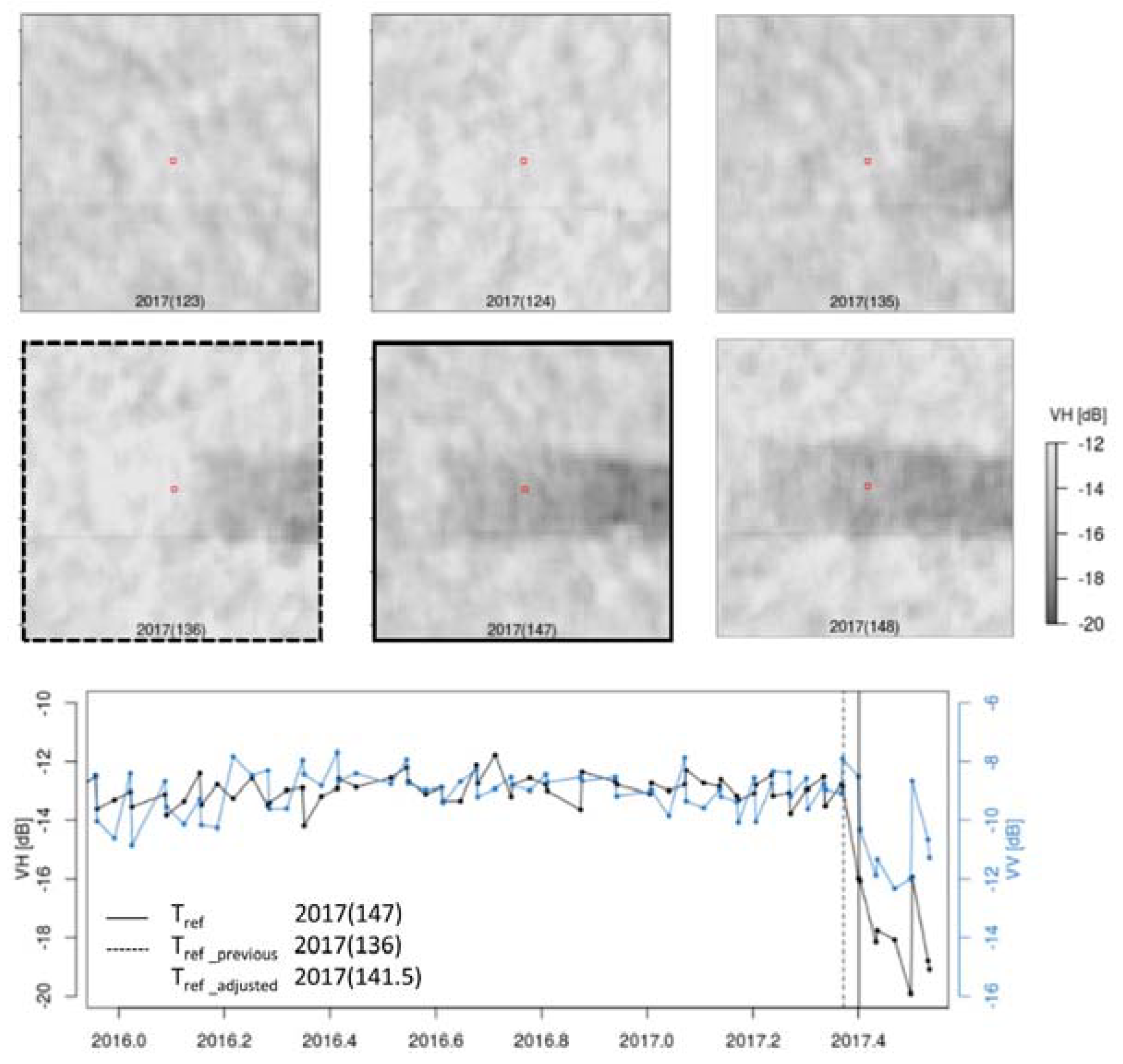
Sample validation pixel (red outline) showing forest-cover loss between 2017 (136) and 2017 (147). The VH backscatter image time series is shown in the top panels and the VH (black) and VV (blue) pixel time series for the validation pixel is shown in the bottom time series graph panel. The pixel time series shows the lower forest/non-forest difference for C-band VV when compared to VH.
Figure 3.
Sample validation pixel (red outline) showing forest-cover loss between 2017 (136) and 2017 (147). The VH backscatter image time series is shown in the top panels and the VH (black) and VV (blue) pixel time series for the validation pixel is shown in the bottom time series graph panel. The pixel time series shows the lower forest/non-forest difference for C-band VV when compared to VH.

Figure 4.
Spatial accuracy (OA, PA and UA of the forest cover loss class), and temporal accuracy (MTL = mean time lag of confirmed forest cover loss events; MTLF = mean time lag of the date at which confirmed forest cover loss events were first flagged) for VV and VH as a function of increasing χ threshold values, separately for natural forest (A) and plantation forest (B).

Figure 5.
Forest-cover loss in Riau, Indonesia detected for the period 1 January 2016–30 January 2017. Areas indicated by (A) and (B) are shown as detailed maps in Figure 6.
Figure 5.
Forest-cover loss in Riau, Indonesia detected for the period 1 January 2016–30 January 2017. Areas indicated by (A) and (B) are shown as detailed maps in Figure 6.

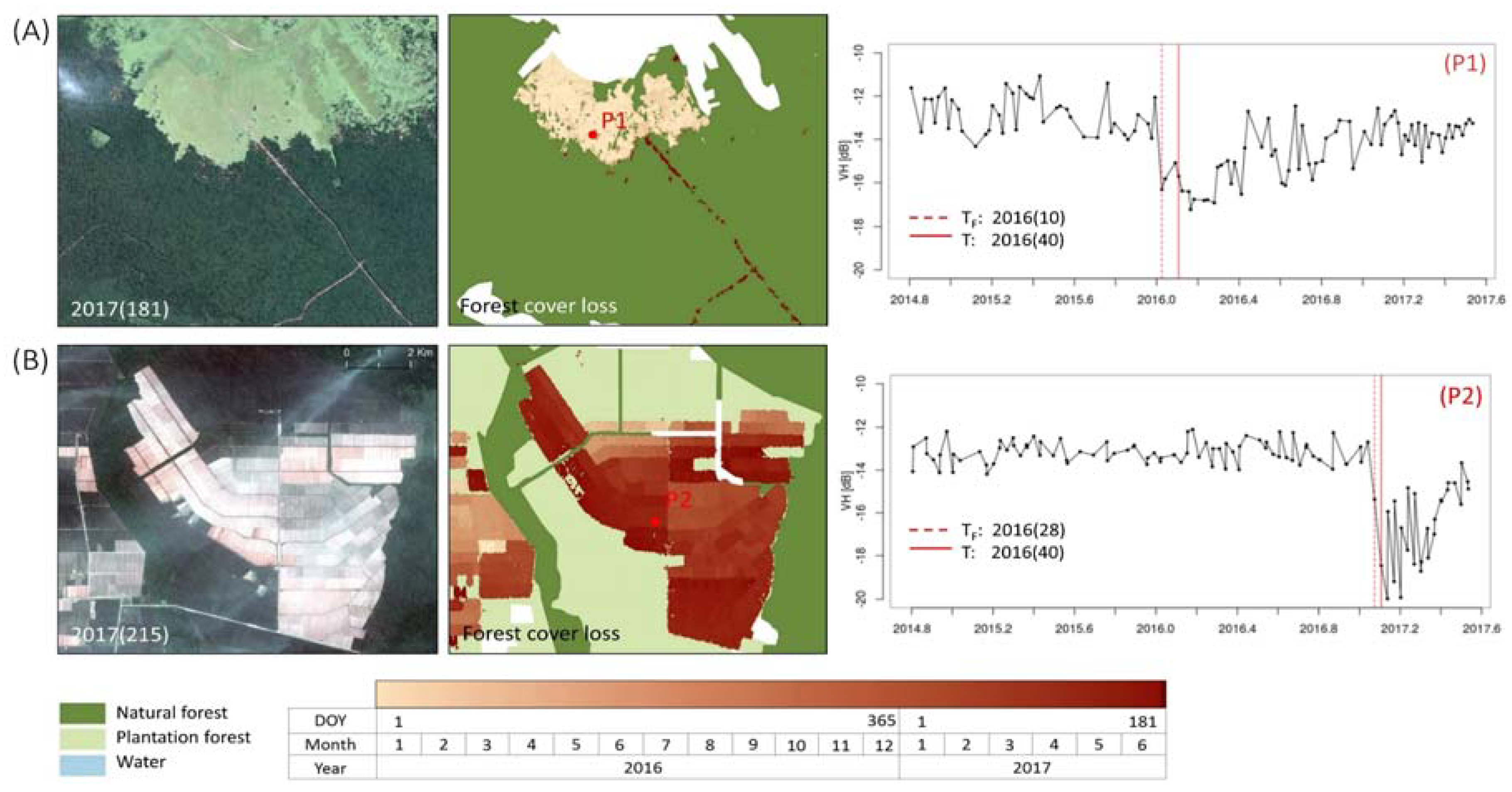
Figure 6.
Detailed maps of forest-cover loss due to (A) encroachment including road construction into natural forest (0.87°N, 102.52°E); and (B) large-scale plantation dynamics (0.56°N, 102.12°E). High resolution satellite images from PlanetScope (3 m resolution, [46]). Example time series (right panel) indicating the dates at which forest-cover loss was flagged (red dotted line) and confirmed (red line).

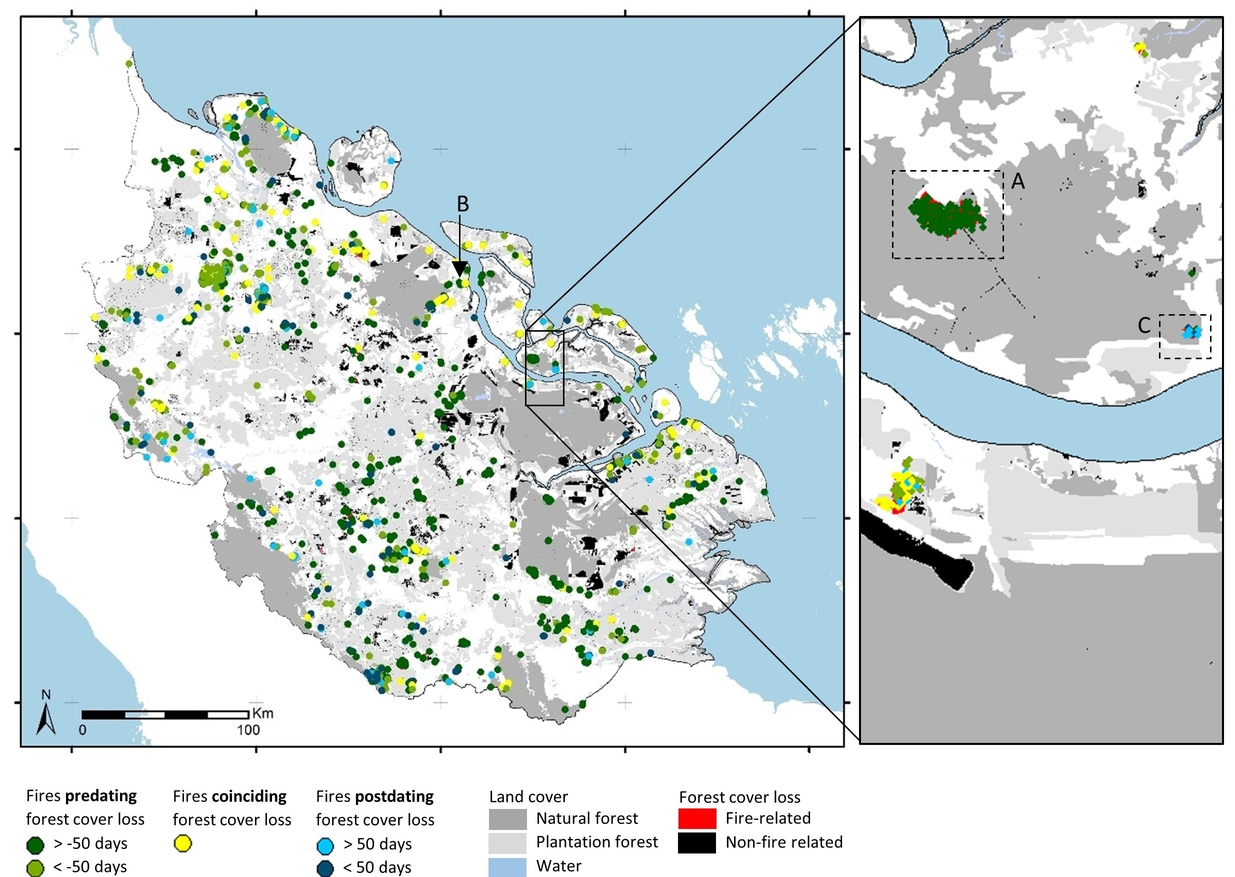
Figure 7.
Fire-related (red) versus non-fire-related forest cover loss (black) in Riau, Indonesia for the period 1 January 2016–30 January 2017. Detail map (right panel) shows an area with partly fire-related forest-cover loss in both natural (dark green) and plantation forest (light green).
Figure 7.
Fire-related (red) versus non-fire-related forest cover loss (black) in Riau, Indonesia for the period 1 January 2016–30 January 2017. Detail map (right panel) shows an area with partly fire-related forest-cover loss in both natural (dark green) and plantation forest (light green).

Figure 8.
Percentage of active fires predating, coinciding with and postdating forest-cover loss, separately for natural (dark grey) and plantation forest (light grey).
Figure 8.
Percentage of active fires predating, coinciding with and postdating forest-cover loss, separately for natural (dark grey) and plantation forest (light grey).

Figure 9.
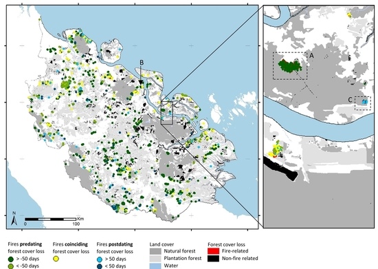
Spatial pattern of fires predating (green), coinciding with (yellow), and postdating (blue) forest-cover loss in Riau, Indonesia. Areas indicated by (A); (B–C) are shown as detailed maps in Figure 10.
Figure 9.
Spatial pattern of fires predating (green), coinciding with (yellow), and postdating (blue) forest-cover loss in Riau, Indonesia. Areas indicated by (A); (B–C) are shown as detailed maps in Figure 10.

Figure 10.
Three examples showing: (A) fire predating forest cover loss in natural forest (0.87°N, 102.52°E); (B) fire coinciding with forest cover loss in plantation forest (1.27°N, 102.14°E); (C) fire predating forest cover loss in natural forest (0.86°N, 102.5°E). High resolution satellite image from PlanetScope (3 m resolution, [46]) (left panel). Pixel time series examples (right panel) indicating the dates at which forest cover loss was flagged (red dotted line) and confirmed (red line), as well as the date of the active fire event (blue line).

© 2018 by the authors. Licensee MDPI, Basel, Switzerland. This article is an open access article distributed under the terms and conditions of the Creative Commons Attribution (CC BY) license (http://creativecommons.org/licenses/by/4.0/).
Share and Cite
MDPI and ACS Style
Reiche, J.; Verhoeven, R.; Verbesselt, J.; Hamunyela, E.; Wielaard, N.; Herold, M. Characterizing Tropical Forest Cover Loss Using Dense Sentinel-1 Data and Active Fire Alerts. Remote Sens. 2018, 10, 777. https://doi.org/10.3390/rs10050777
AMA Style
Reiche J, Verhoeven R, Verbesselt J, Hamunyela E, Wielaard N, Herold M. Characterizing Tropical Forest Cover Loss Using Dense Sentinel-1 Data and Active Fire Alerts. Remote Sensing. 2018; 10(5):777. https://doi.org/10.3390/rs10050777
Chicago/Turabian StyleReiche, Johannes, Rob Verhoeven, Jan Verbesselt, Eliakim Hamunyela, Niels Wielaard, and Martin Herold. 2018. "Characterizing Tropical Forest Cover Loss Using Dense Sentinel-1 Data and Active Fire Alerts" Remote Sensing 10, no. 5: 777. https://doi.org/10.3390/rs10050777
Note that from the first issue of 2016, this journal uses article numbers instead of page numbers. See further details here.