Estimation of Surface Duct Using Ground-Based GPS Phase Delay and Propagation Loss

Abstract

The propagation of Global Positioning System (GPS) signals at low-elevation angles is significantly affected by a surface duct. In this paper, we present an improved algorithm known as NSSAGA, in which simulated annealing (SA) is combined with the non-dominated sorting genetic algorithm II (NSGA-II). Matched-field processing was used to remotely sense the refractivity structure by using the data of ground-based GPS phase delay and propagation loss from multiple antenna heights. The performance was checked by simulation data with and without noise. In comparison with NSGA-II, the new hybrid algorithm retrieved the refractivity structure more efficiently under various noise conditions. We then modified the objective function and found that matched-field processing is more effective than the conventional least-squares method for inferring the refractivity parameters. Comparing the inversion results and in situ sounding data suggests that the improved method presented herein can capture refractivity characteristics in realistic environments.

1. Introduction

An atmospheric duct is an atmospheric layer in which strong vertical gradients of refractivity determined by temperature and humidity affect the propagation of electromagnetic waves. The electromagnetic waves are trapped within the ducting layer with weak propagation loss and enhanced propagation range, usually known as atmospheric ducting [1,2]. Turton et al. [3] presented a classification of different radio-propagation conditions and corresponding atmospheric ducting effects. They pointed out that ducting may be associated with the following five meteorological processes: (1) sea-surface evaporation, (2) anticyclonic subsidence, (3) subsidence of cold air beneath frontal surfaces, (4) nocturnal radiative cooling over land, and (5) advection. A strong temperature inversion is often present at the top of a well-mixed marine boundary layer in these meteorological processes [4]. Obviously, there exists a correlation between ducting and boundary-layer inversion. When warm and dry air masses from land travel over cooler water, there exists sharp differences of temperature and humidity vertically, which may result in ducting formation. Propagation loss for radar radio waves within a duct will usually be much less than that in a non-ducting atmospheric environment, and hence radar can detect targets at greater distances. A radar “hole” may also appear just above the duct because of short detection ranges [5]. These characteristics have significant impacts on radar target detection and target tracking because failure to consider a ducting environment may yield false radar returns. Therefore, the study of atmospheric ducts can not only improve the performance of radar or communications systems but can also contribute to research into the atmospheric boundary layer [6,7,8,9].

It is a difficult problem to quantify the patterns of an atmospheric duct in time and space. The methods of sounding refractivity profiles—such as radiosondes, microwave refractometers, and evaporation duct sensors—have been developed [10,11,12,13,14]. However, these methods are direct sensing techniques and have lower sparse sampling rates. Krolik and Tabrikian [15] first used radar clutter data to retrieve atmospheric refractivity profiles. Afterward, the technique of refractivity from clutter (RFC) was developed substantially. A variety of intelligent algorithms have been used to estimate refractivity profiles, for example, the genetic algorithm (GA) [16,17], the Bayesian-Markov-chain Monte Carlo method [18], the support vector machine [19], and others [20,21,22,23]. However, these algorithms have some defects in practical applications [24,25].

A promising approach for sensing refractivity profiles remotely is the use of Global Positioning System (GPS) signals [10,26]. Hitney [27] demonstrated the capability of estimating the trapping layer’s base height from ultrahigh frequency (UHF) signal strengths. Anderson [28] inferred the refractivity structure in the lower atmosphere based on the phase delay from a ground-based GPS receiver as the satellite rose or set on the horizon. Lowery et al. [29] and Lin et al. [30] estimated the refractivity structure using a ray-tracing model to fit measured GPS phase delays with least-squares and evaluated the potential and limitations of this method [31]. Subsequently, other scholars [32,33] also inferred refractivity profiles from measured excess phase path. However, only one type of observational data is used in these methods, such as the GPS signal strength or phase delay. Therefore, Wu et al. [34] tried to combine the GPS phase delay and bending angle to retrieve refractivity profiles, but they neglected the fact that the observed phase delay and bending angles are not independent. For this reason, Liao et al. [35] used the non-dominated sorting genetic algorithm II (NSGA-II) to retrieve the atmospheric refractivity structure based on the ground-based GPS phase delay and propagation loss. Although the combination of ground-based GPS phase delay and propagation loss can infer refractivity parameters effectively, its performance is limited by the weak global search capability of NSGA-II. Therefore, in the present paper, we propose an improved algorithm based on NSGA-II in which the method of electromagnetic match-field processing is applied [36]. Furthermore, we also integrate the GPS phase delay and propagation loss from multiple antenna heights to infer the refractivity parameters.

The present paper is a sequel to Liao et al. [35] and is aimed at quantifying the performance of the joint inversion for two types of observation using improved NSGA-II. Here, the objective function is match-field processing. The remainder of this paper is organized as follows. Section 2 introduces the forward model, including models of GPS phase delay and radio signal propagation. Section 3 proposes a new algorithm—the non-dominated sorting and simulated annealing genetic algorithm (NSSAGA)—which is an improved version of NSGA-II that includes simulated annealing (SA), and it describes the algorithm implementation step by step. Section 3 also introduces a simplified mathematical model of a surface duct and a related objective function. Section 4 presents the NSSAGA algorithm used for refractivity-profile estimation. Finally, conclusions from this work are summarized in Section 5.

2. Forward Model

2.1. Phase-Delay Model

In this section, some basic concepts regarding the ground-based GPS phase-delay model are introduced briefly. Because of variations in atmospheric temperature $T$, pressure $P$, and water vapor pressure $e$, the atmospheric refractivity $N$ is approximated by a formula due to Smith and Weintraub [37]:

$$N=77.6\times p/T+3.73\times {10}^5\times (e/T^2)$$

(1)

where the unit of $T$ is K and the unit of $P$ and $e$ is hPa. The modified refractivity $M$, which considers the Earth’s curvature, is related to the radio refractivity $N$ as follows [38]:

$$M=N+0.157\times r$$

(2)

Differentiating with respect to $r$, we get

$$dM/dr=dN/dr+0.157$$

(3)

where $r$ is the altitude in meters and $M$ is the modified refractivity. The unit of $dM/dr$ is M-units/km. Equations (2) and (3) are applied for all radio frequencies with little error. Referring to Almond and Clarke [39], $dN/dr$—which is the gradient of refractivity $N$ with respect to altitude $r$—is used to classify the profiles and its unit is N-units/km. Normally, the atmospheric refractivity has a negative gradient when the electromagnetic waves bend toward the Earth. However, if the refractivity gradient is less than −160 N-units/km, an atmospheric duct occurs. The atmospheric structure, especially a surface duct, may delay the GPS signal at low elevation. Hence, this study used the GPS phase delay to retrieve the surface duct.

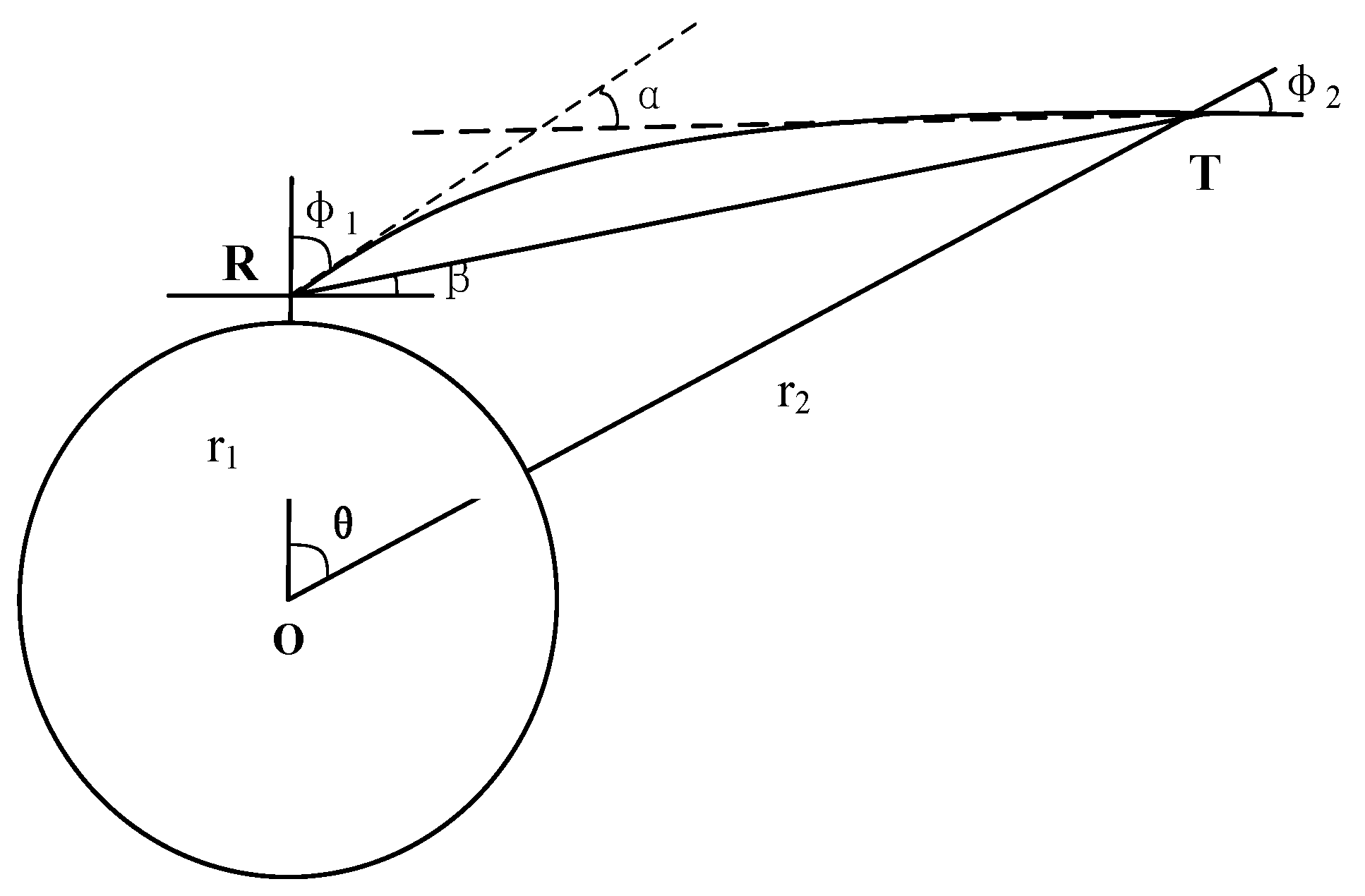
Figure 1 shows the geometry of the ray path in a ground-based GPS occultation, where $R$ and $T$ are the GPS receiver and transmitter, respectively, and $r_1$ and $r_2$ are the distances from the geocenter $O$ to the receiver and transmitter, respectively.

Assuming that the atmosphere is a spherically symmetric and layered refractive medium, the GPS signal path is approximated as a function of $r$ only. The phase path is determined according to Sheng et al. [32]:

$$S={\displaystyle \underset{r_1}{\overset{r_2}{\int }}n(r)dl}$$

(4)

where $dl=\sqrt{d{r}^2+r^{2}d{\theta }^2}$ is a differential length along the ray path and $n$ is the refractive index with $N=(n-1)\times {10}^6$. Using Bouger’s law—namely, $a=nr\sin \phi$, where $a$ is a constant impact parameter associated with the ray path—and substituting $dl=dr/\cos \phi$, Equation (4) can be represented as:

$$S={\displaystyle \underset{r_1}{\overset{r_2}{\int }}r\cdot n^2/\sqrt{r^2\cdot n^2-a^2}}dr={\displaystyle \underset{x_1}{\overset{x_2}{\int }}x\cdot \left[1-(x/n)dn/dx\right]/\sqrt{x^2-a^2}}dx$$

(5)

where $x=rn(r)$ denotes the refractive radius. The ray path in a vacuum can be determined as:

$$S_0=\sqrt{r_1^2+r_2^2-2r_{{}^1}\cdot r_2\cdot \cos \theta }$$

(6)

where the angle $\theta$ is the spherical angle between $r_1$ and $r_2$. Hence, the excess phase path is defined as:

$$\Delta S=S-S_0$$

(7)

2.2. Propagation-Loss Model

To use the propagation loss of ground-based GPS, a forward-propagation model is established. The electromagnetic wave propagation equation (PE), derived from the wave equation by the parabolic approximation, is widely used to model refractive effects on GPS signal propagation [40]. Teti [41] explains the PE theory in detail. Considering the spherical shape of the Earth, the two-dimensional (2D) narrow-angle forward PE can be written as:

$$\partial u(x,z)/\partial x=i/(2\cdot k)\cdot {\partial }^{2}u(x,z)/\partial z^2+i\cdot k/2\cdot (M^2(x,z)-1)\cdot u(x,z)$$

(8)

where $x$ and $z$ represent the horizontal axis (range) and the vertical axis (height), respectively, $k$ is the wavenumber in free space, $M(x,z)$ is the modified refractivity, and $u(x,z)$ is the electromagnetic field component at range $x$ and height $z$. Equation (8) can be used for both horizontal and vertical polarization.

If the initial field is provided, the split-step Fourier transform (SSFT) is used to calculate low-elevation GPS signal propagation in a tropospheric duct. This can be substituted by a sine or cosine transform because the bottom boundary approximates to a perfectly conducting surface. The SSFT solution of propagated wave equation is expressed as [26]:

$$u(x+\Delta x,z)=\exp (ik(M^2-1)\Delta x/2)F^{-1}\{\exp (-i{\pi }^2{p}^2\Delta x/(2k))F[u(x,z)]\}$$

(9)

where $F$ and $F^{-1}$ are the Fourier transform and inverse Fourier transform, respectively. Here, $\Delta x$ is the range step, $p=2k\sin \theta$ represents the transform variable for which $\theta$ is the angle from the horizontal, and $u(x,z)$ is the initial field. Balvedi and Walter [42] give a more detailed process for solving the parabolic equation.

To model the GPS signal propagation, the single-way propagation loss $L(x,z)$ of ground-based GPS signals is used to describe the objective function [18]:

$$L(x,z)=20\log (f)+20\log (x)+C$$

(10)

where $f$ represents the propagation factor and $C$ is a constant parameter. In a rectangular coordinate system, the propagation can be calculated as:

$$f=\sqrt{x}\left|u(x,z)\right|$$

(11)

3. Improved Inversion Algorithm

3.1. Proposed NSSAGA Algorithm

Combining the GPS phase delay and propagation loss is a multiobjective optimization process. Hence, we used NSGA-II—a multiobjective optimization algorithm—to search for the best fit [35,43]. Considering that NSGA-II is an improvement of NSGA, one of the first evolutionary algorithms (EAs) for finding multiple Pareto-optimal solutions, the former retains premature convergence, which is a common problem with conventional GAs. In other words, the solving procedure becomes trapped at a local optimum and the inversion parameters converge to a suboptimal solution [44].

The SA algorithm was first proposed by Metropolis et al. [45]. It is based on the physical principle of heating a material and then slowly lowering the temperature to decrease defects, further minimizing the system energy [46]. SA is a probabilistic technique for approximating the global optimum of a given function. Combining SA and NSGA-II could overcome premature convergence effectively and find the global optimum instead of a local one [47]. Therefore, we combined them into a hybrid algorithm, namely, NSSAGA, that we used for surface-duct retrieval.

3.2. Implementation Steps

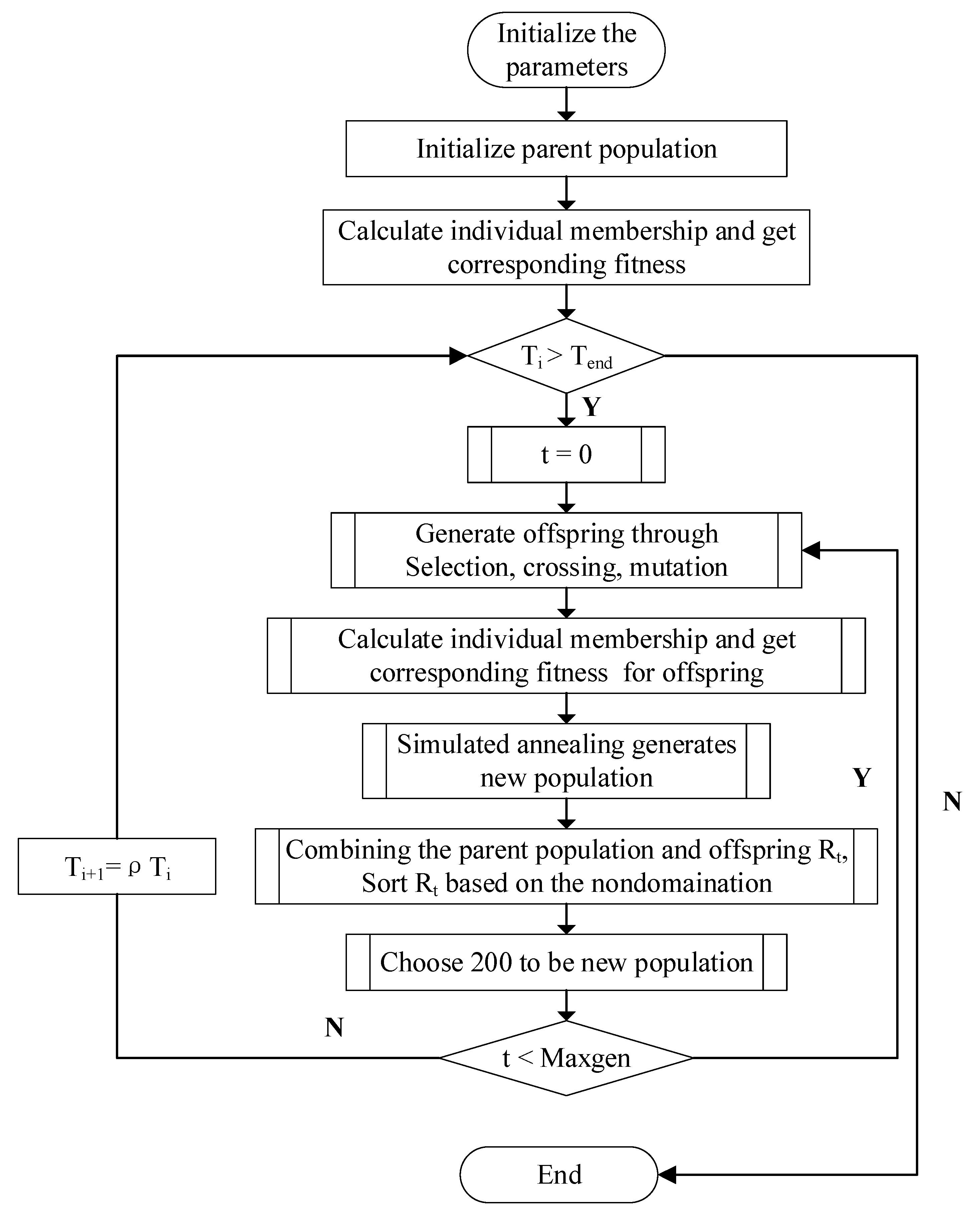
Based on the above ideas, the procedure of the proposed hybrid algorithm is shown in Figure 2. The detailed design steps for parameter estimation by the NSSAGA algorithm are realized as follows.

Step 1: Initialize the parameter values of the hybrid algorithm. The population size is 200 and the maximum number of generations is set to 10. In NSSAGA, the population size is the number of candidate solutions and the number of generations is the number of program iterations. The numbers of objective functions and variable parameters in the program are set to 2 and 4, respectively. A variable parameter is a physical variable to be inverted. For the real-coded NSSAGA, a multi-parent extension of the simulated binary crossover (SBX) operator is used, and the distribution indexes for the crossover and mutation operators are set to ${\eta }_c=20$ and ${\eta }_m=20$, respectively. The crossover and mutation operators ${\beta }_i$ are defined by

$${\beta }_i=\{\begin{array}{c}(2u_i{)}^{1/(\eta +1)}\\ {[1/(2(1-u_i))]}^{1/(\eta +1)}\end{array}\begin{array}{c}if{u}_i\le 0.5\\ Otherwise\end{array}$$

(12)

Here, $u_i$ determines the probability of crossing or mutating and is chosen randomly from the interval [0,1], where $i$ is the generation number. We set the initial temperature as $T_o=100$ and the end temperature as $T_{end}=0$. The cooling factor $\rho$ is 0.8, determining the rate of change of temperature required in SA.

Step 2: Initially, a parent population $P_t=[x_1,x_2,x_3,\cdots ,x_{200}]$ is generated randomly within the boundaries of the solution while calculating the corresponding function value. The SA time $i$ is zero.

Step 3: Begin the main loop. If the SA condition $T_i>T_{end}$ is met, we set the generation variable as $t=0$. Otherwise, the program ends.

Step 4: The usual binary tournament selection, cross operators, and mutation operators are used to create an offspring $Q_t=[x_1,x_2,x_3,\cdots ,x_{200}]$ with the corresponding function value. Here, the usual binary tournament selection involves running several “tournaments” among a few individuals chosen at random from the population.

Step 5: The Metropolis criterion is the core of the SA algorithm, which derives from the importance-sampling method proposed by Metropolis et al. [45]. Designing the system energy $E$ as the function value $J$, let $\Delta =J_{new}-J_{old}$ and move the system to the new state if the random variable $p$, distributed uniformly over (0,1), satisfies

$$p\le \exp (-\Delta /T_i)$$

(13)

where $T_i$ is the current temperature.

Step 6: A combined population $R_t=P_t\cup Q_t$ is formed, where $R_t$ = 400. In a typical multiobjective optimization problem, there exists a set of solutions that are superior to the other solutions in the search space when all objectives are considered but are inferior to other solutions in the space in one or more objectives. These solutions are called as non-dominated solutions [46]. The population $R_t$ is sorted based on the non-domination levels, and 200 individuals in the population $R_t$ are chosen to be the new parent population $P_{t+1}$. We update the generation variable $t=t+1$ and archive the best individual in the new population to the vector $P_{t,best}$. If the iteration condition meets $t<Maxgen$, repeat Steps 4–6. Otherwise, we achieve the best individual from $P_{t,}{}_{best}$ to $S_{i,best}$ and repeat Steps 3–6, updating the number $i=i+1$.

Step 7: Once we have completed Steps 3–6 and the SA condition $T_i<T_{end}$ is met, the process stops, and the system is considered to have frozen to the lowest temperature as defined by the annealing schedule. Output the best of $S_{i,best}$.

3.3. Modeling Refractivity Profile and Objective Function

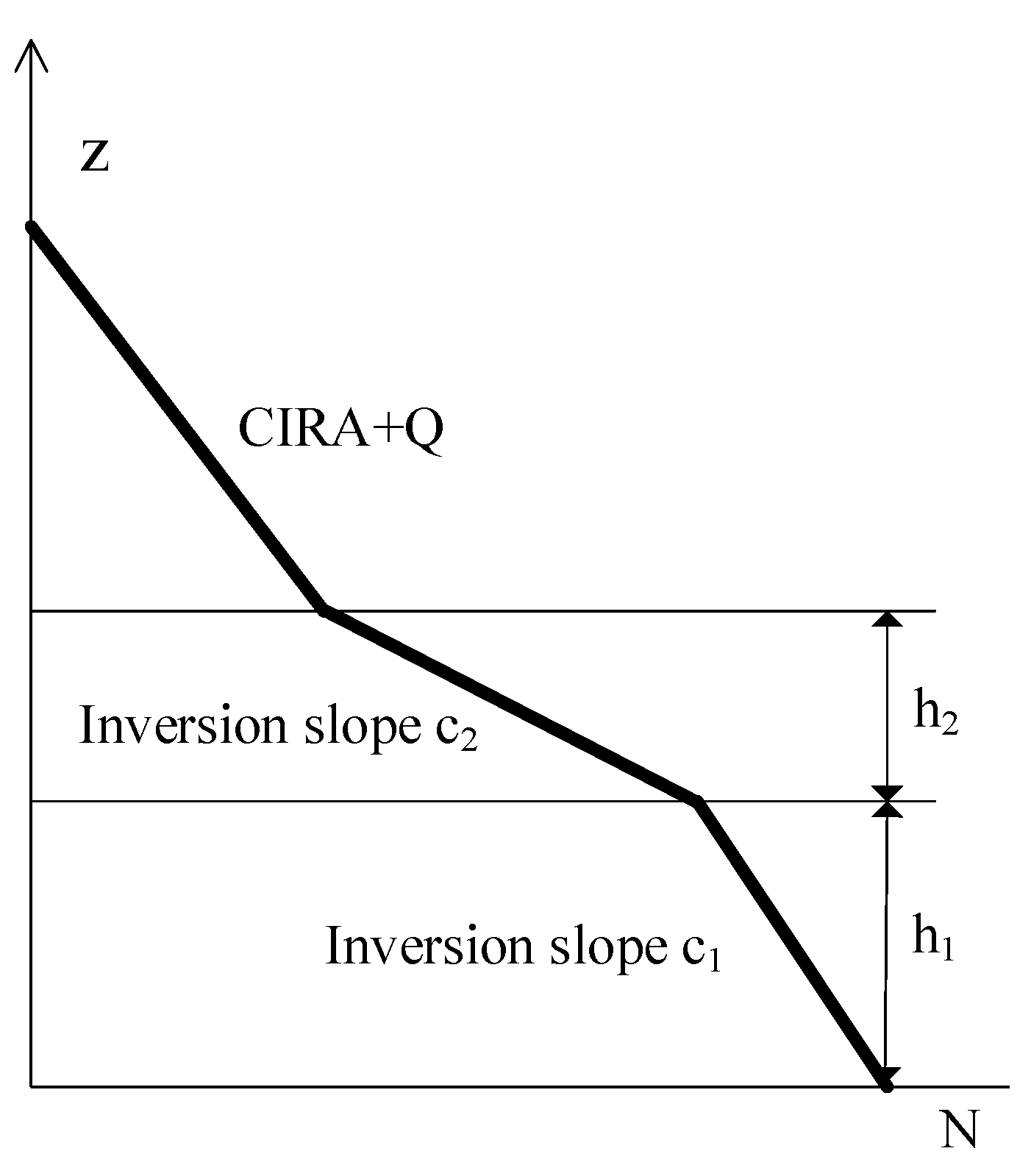
A surface duct always forms when a relatively warm, dry air mass travels over a cooler, moister air mass [26], and it may cause substantial errors in propagation calculations for low-elevation GPS signals [47]. The modified refractivity profile is commonly employed for a surface duct. The following is a four-parameter trilinear model [48] that parameterizes the atmospheric refractivity structure (Figure 3):

$$M(z)=M_0+\{\begin{array}{c}{c}_{1}z\\ c_1{h}_1+c_2(z-h_1)\\ c_1{h}_1+c_2{h}_2+0.118z\end{array}\begin{array}{c}z<h_1\\ h_1<z<h_1+h_2\\ z>h_1+h_2\end{array}$$

(14)

where $h_1$ is the trapping-layer based height, $c_1$ is the base slope, $h_2$ is the inversion-layer thickness, and $c_2$ is the slope from $h_1$ to $h_1+h_2$. The slope of the top layer is 0.118 M-units/m, considering the layer as the standard refractivity condition.

To reconstruct the refractivity profile, a multiobjective cost function [35] (Liao et al., 2016) is usually defined as:

$$\{\begin{array}{c}{J}_1(\mathbf{x})={(\Delta S{(\mathbf{x})}^{obs}-\Delta S{(\mathbf{x})}^{\mathrm{mod}})}^2=\min !\\ J_2(\mathbf{x})={(P_c{(\mathbf{x})}^{obs}-P_c{(\mathbf{x})}^{\mathrm{mod}})}^2=\min !\end{array}$$

(15)

where $\mathbf{x}={(c_1,c_2,h_1,h_2)}^{\mathrm{T}}$ is a vector, $\Delta S{(\mathbf{x})}^{obs}$ and $\Delta S{(\mathbf{x})}^{\mathrm{mod}}$ are the observed and simulated GPS phase delays, respectively, at the same antenna height, and $P_c{(\mathbf{x})}^{obs}$ and $P_c{(\mathbf{x})}^{\mathrm{mod}}$ are the observed and received GPS propagation losses, respectively, at the same antenna height. Here, the objective function is the least-squares function. However, the ordinary least-squares (OLS) function cannot be minimized directly when the parameters acquire small errors in some cases.

The Bartlett objective function, which is broadly used in the field of marine acoustic tomography, achieves good results in estimating refractivity conditions [10]. Hence, we adopted the Bartlett power function as the new cost function. Referring to Gerstoft et al. [10], the objective function is defined as:

$$\{\begin{array}{c}{J}_1(\mathbf{x})={(\Delta S{(\mathbf{x})}^{obs}-\Delta S{(\mathbf{x})}^{\mathrm{mod}})}^2=\min !\\ J_2(\mathbf{x})=\frac{1}{N_{dep}{N}_{element}}{\displaystyle \sum _{k=1}^{N_{dep}}{\displaystyle \sum _{i=1}^{N_{element}}[{{\displaystyle \sum _{j=1}^{N_x}\left|p_{i,j,k}\right|}}^2-\frac{\left|{\displaystyle \sum _{j=1}^{N_x}{P}_{i,j,k}^T{Q}_{i,j,k}}\right|}{{\displaystyle \sum _{j=1}^{N_x}{Q}_{i,j,k}}}]}}=\min !\end{array}$$

(16)

where $P_{i,j,k}$ and $Q_{i,j,k}$ are the observed and calculated data, respectively, in dB form; they are the elements of the propagation loss matrices. Term $N_{dep}$ is the height, $N_x$ is the range, and $N_{element}$ is the number of GPS receivers at the same antenna height. Here, the receiver heights are 20 m, 50 m, 100 m, 150 m, and 400 m. There is only one receiving antenna at a given height level.

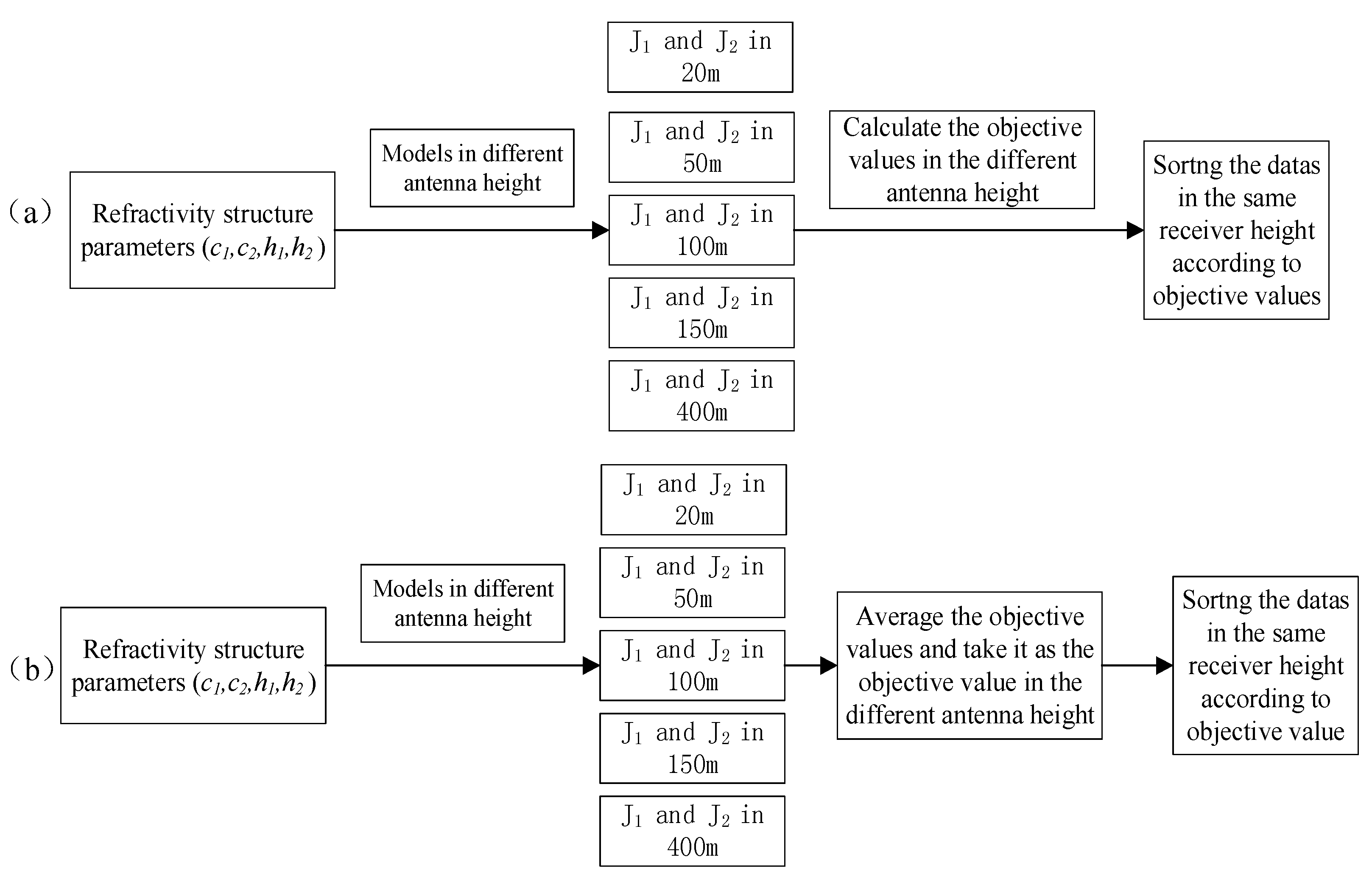
Section 3.2 noted that the population is sorted by the solutions sets $J_1$ and $J_2$ according to non-domination. For different antenna heights, the same values of the refractivity parameters may produce a different set of solutions. Thus, when inferring refractivity parameters based on data sets collected from antenna of differing height, we must sort the individuals according to whether the height dependence of the data (phase delay and propagation loss) is considered. Considering the change in receiver height means that each datum from an antenna of a given height calculates its own objective function, whereupon individuals associated with the same height are sorted according to their objective values (Figure 4a). Otherwise, we take the average objective value of the different antenna heights and take it as the objective function of data sets with different antenna heights, sorting individuals associated with the same height according to Figure 4b. Finally, the inversion method must average the optimal parameters $S_{i,best}$ from the different heights as the final result.

Herein, we define the Bartlett function as Bartlett1 if we consider the receiver height or as Bartlett2 if we do not. In contrast to the Bartlett function, the OLS function, which considers the change in receiver height, is taken into account in Section 4 as part of the NSSAGA-OLS algorithm.

4. Results

The simulations assumed a GPS elevation angle of 1°, a transmitting frequency of 1500 MHz, and a beam width of 16°. To verify the feasibility and anti-noise ability, the simulated conditions contain 0%, 3%, 5%, 7%, or 10% Gaussian white noise; the 0% level is the ideal condition. Here, the Gaussian white noise was added into the propagation loss only and the phase delay is kept accurate. However, the elevation angle seriously affects the error of phase delay. This uncertainty is estimated to be about 8–10 mm from the zenith, increasing to about 8–10 cm at an elevation angle of 5° [49]. Therefore, noise of delay information is also necessary to consider and becomes the follow-up research.

4.1. Comparison between NSSAGA and NSGA-II

In this section, we compare the performance of NSSAGA with that of NSGA-II, using the same objective function and the same receiver height. Here, the objective function is Equation (15).

Table 1. The value of inversion parameters under noiseless and added noise conditions (bold font indicates best retrieved parameters).

Parameters		Inversion Slope c1	Height h1	Inversion Slope c2	Height h2
Units		N-units/m	m	N-units/m	m
Lower bound		−0.1	50	−0.4	250
Upper bound		0	150	0	350
True value		−0.02	100	−0.2	300
NSSAGA	20 m	−0.0302 (51%)	107.4749 (7.5%)	−0.1979 (−1.1%)	296.8430 (−1.1%)
	100 m	−0.0524 (162%)	116.8249 (16.8%)	−0.1894 (−5.3%)	295.6861 (−1.4%)
	150 m	−0.0264 (32%)	104.6840 (4.7%)	−0.1952 (−2.4%)	305.6387 (1.9%)
	400 m	−0.0414 (107%)	106.5472 (6.6%)	−0.1966 (−1.7%)	286.0859 (−4.6%)
NSGA-II	20 m	−0.0247 (23.5%)	51.3844 (−48.6%)	−0.2103 (5.2%)	288.6211 (−3.8%)
	100 m	−0.0615 (207.5%)	83.1727 (−16.8%)	−0.2213 (10.7%)	255.8522 (−14.7%)
	150 m	−0.0767 (283.5%)	111.1971 (11.2%)	−0.1633 (−18.4%)	326.9079 (9.0%)
	400 m	−0.0021 (−89.5%)	77.9154 (−22.1%)	−0.2430 (21.5%)	253.9479 (−15.4%)

lists the limits of inverting parameters and the true values. The inversion results for different antenna heights are also given in Table 1. From Table 1, the synthetic parameters retrieved by NSSAGA are better than those retrieved by the compared algorithm NSGA-II for the same antenna height under the ideal condition. Moreover, it is difficult to compare the inversion results for different antenna heights using the same algorithm.

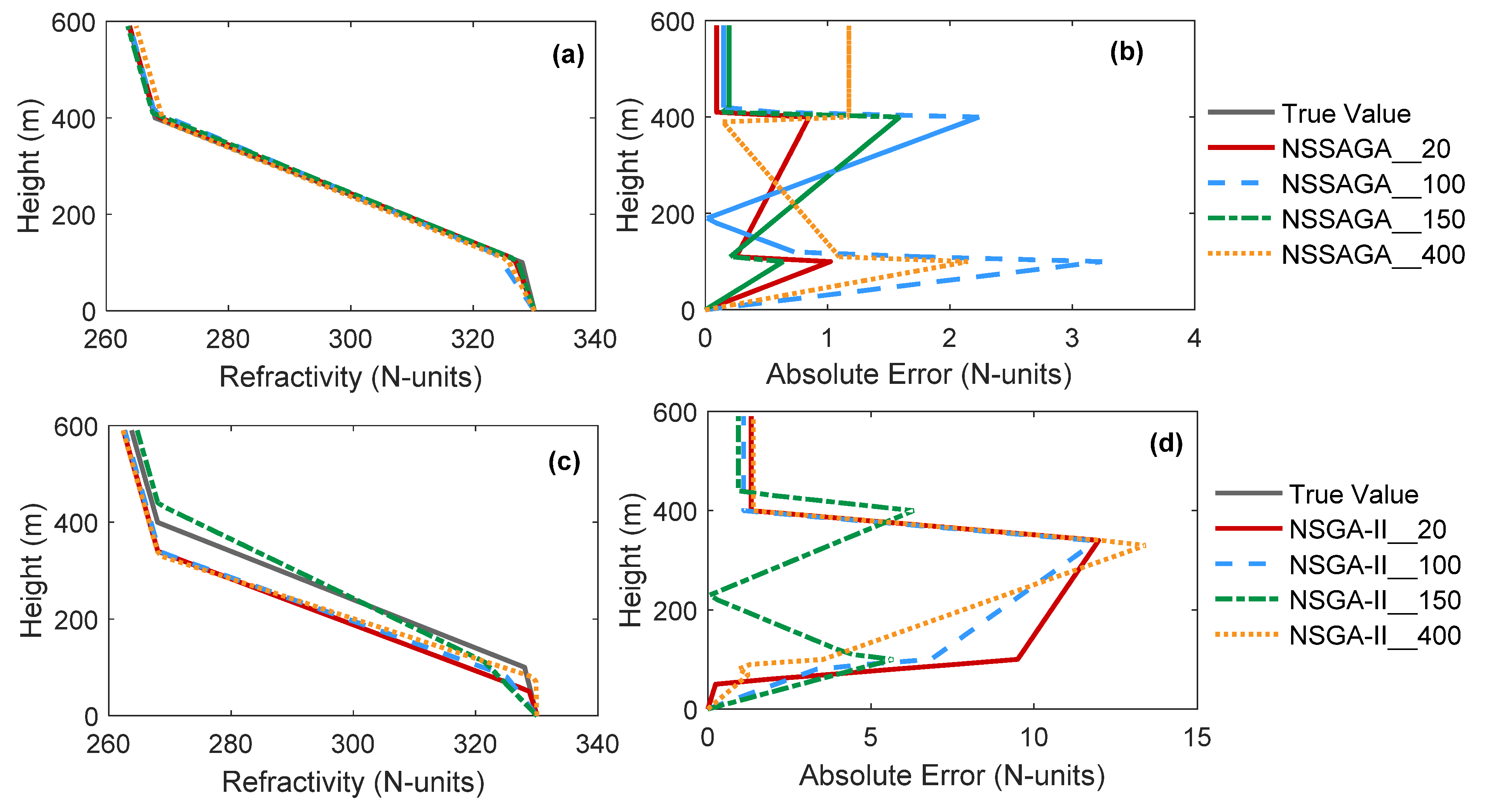
Figure 5 illustrates the retrieved refractivity profile and the corresponding absolute error. The numbers in the legends represent the antenna height. Because the discrepancy between the retrieved and simulated profiles is large for the antenna height of 50 m, Figure 5 gives the retrieved profile excluding its results. Obviously, the retrieved profile based on NSSAGA for the same antenna height is closer to the real profile than those based on NSGA-II. The absolute error also shows that NSSAGA performs better than NSGA-II. The error of NSSAGA_20 versus height is less than 1 N-unit, while the error of NSSAGA_150 is less than that of the other algorithms except NSSAGA_20. Thus, the best retrieval results are achieved when the receiver is located inside the duct. In general, the new algorithm NSSAGA outperforms NSGA-II in multiobjective inversion. In other words, adding the SA algorithm has improved NSGA-II.

4.2. NSSAGA with Different Levels of Gaussian Noise

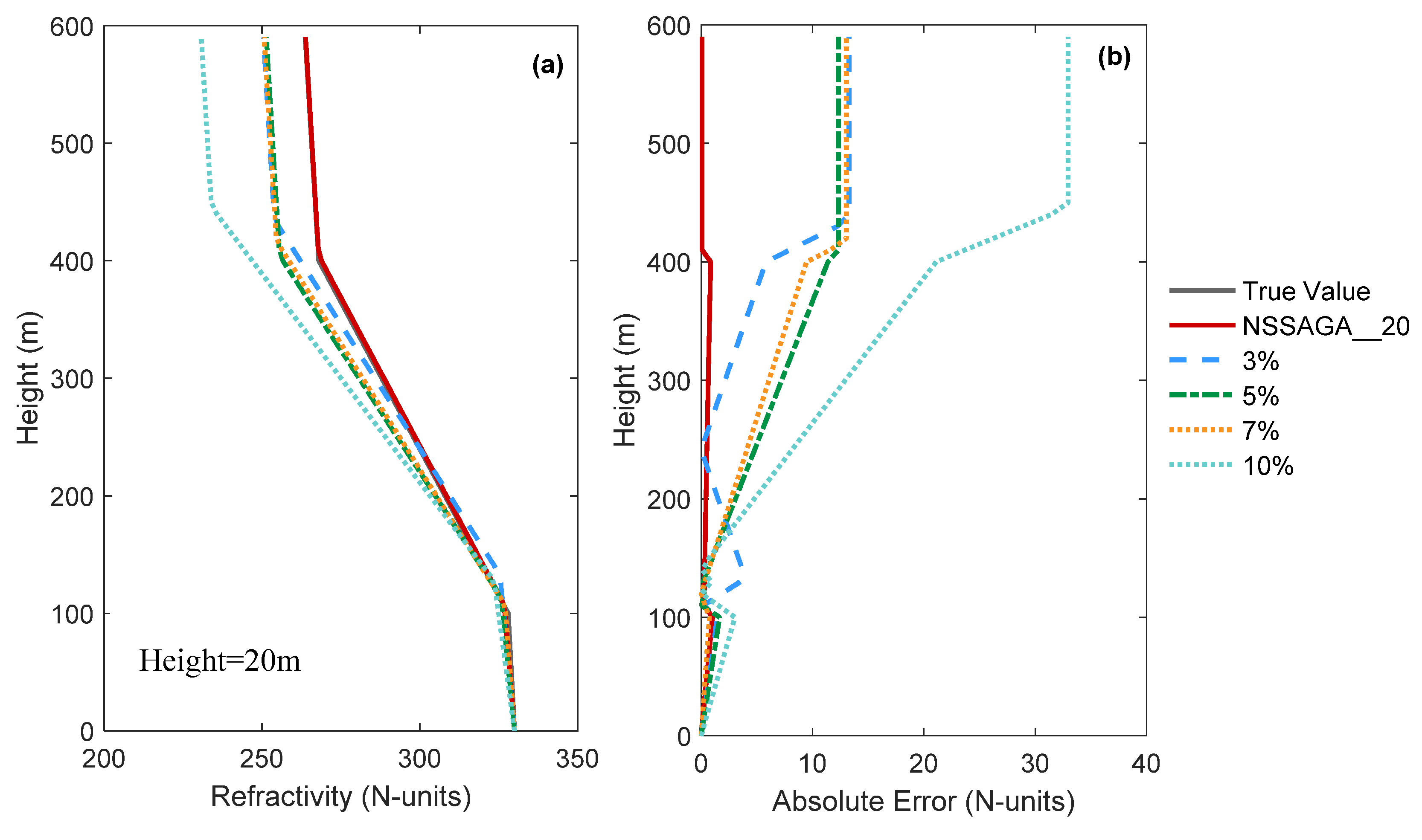
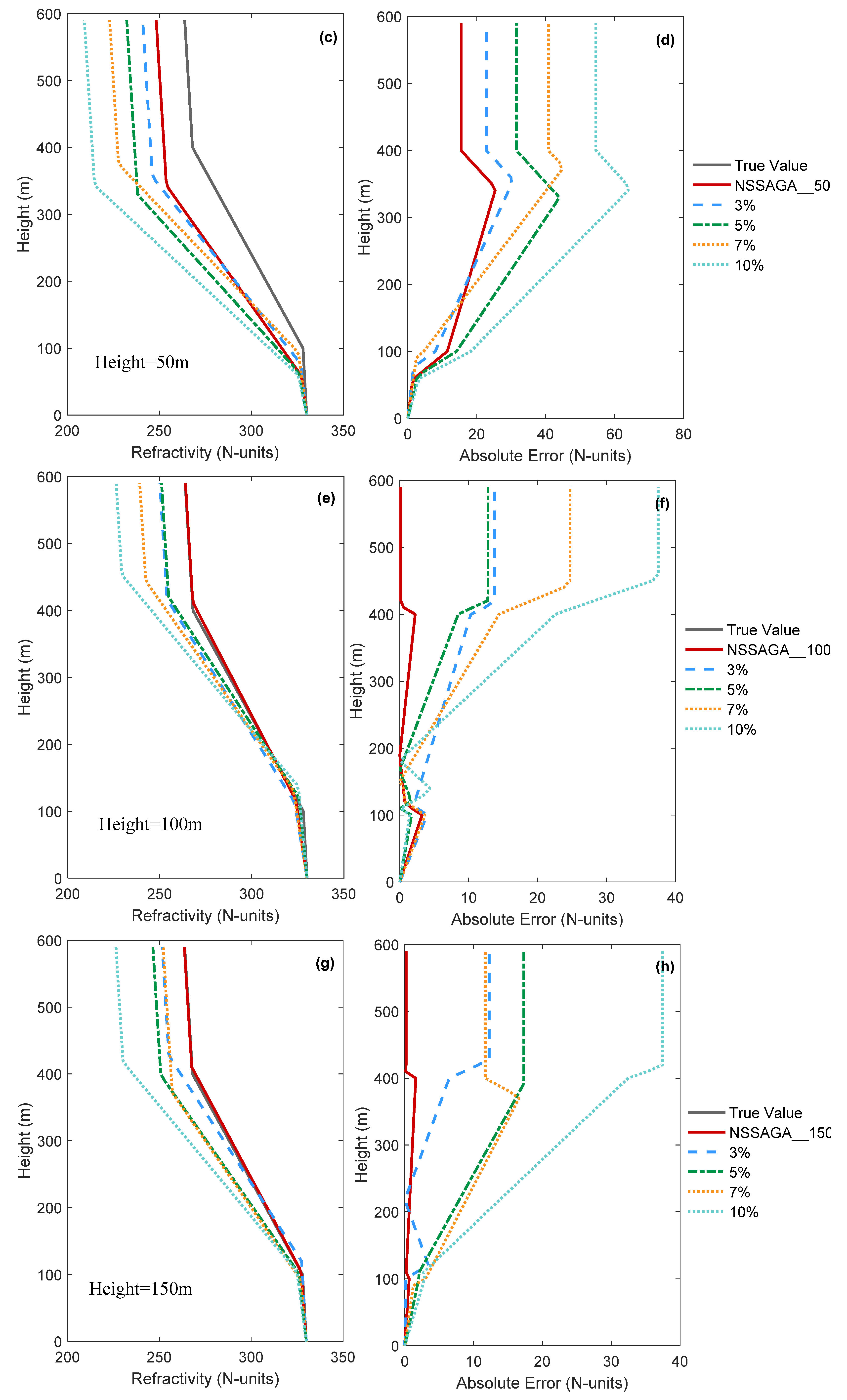
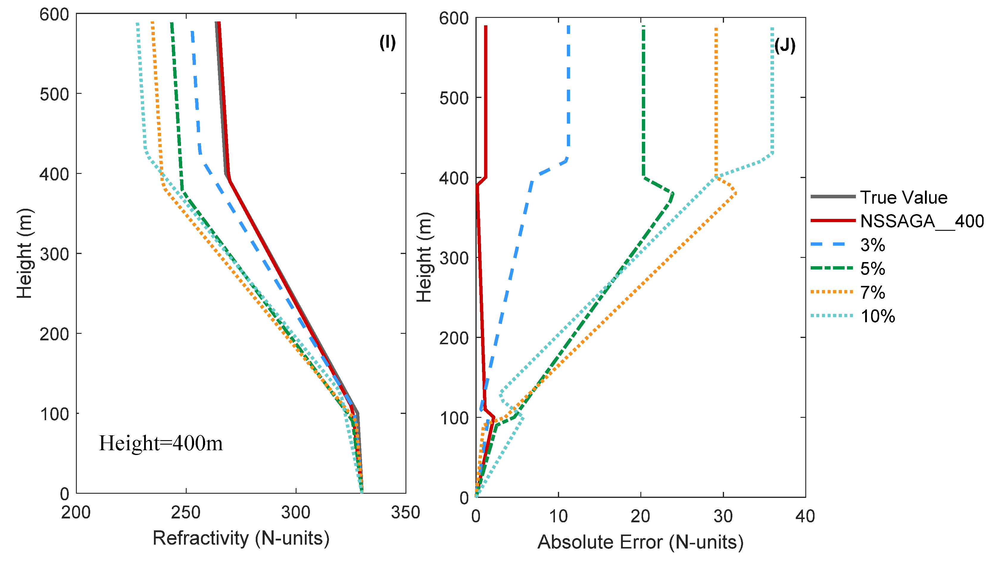
Most practical applications of GPS observations involve measurement errors. In this section, we present retrieval simulations that involve measurement errors that we assume obey Gaussian statistics. The detailed retrieval results are presented in Figure 6 and

Table 2. The value of inversion parameters under different antenna heights and Gaussian noise levels (bold font indicates best retrieved parameters).

Antenna Height and Gaussian Noise Level		Inversion Slope c1	Height h1	Inversion Slope c2	Height h2
20 m	3%	−0.0345 (72.5%)	132.8208 (32.8%)	−0.2367 (18.4%)	302.0072 (0.7%)
	5%	−0.0366 (83%)	113.3292 (13.3%)	−0.2415 (20.8%)	290.9717 (−3%)
	7%	−0.0274 (37%)	106.8854 (6.9%)	−0.2338 (16.9%)	310.0565 (3.4%)
	10%	−0.0504 (152%)	127.7177 (27.7%)	−0.2816 (40.8%)	318.0503 (6%)
50 m	3%	−0.0419 (109.5%)	76.6365 (−23.4%)	−0.2886 (44.3%)	279.2205 (−6.9%)
	5%	−0.0650 (225%)	63.5319 (−36.5%)	−0.3299 (65.0%)	265.9958 (11.3%)
	7%	−0.0476 (138%)	93.6565 (−6.3%)	−0.3476 (73.8%)	281.2179 (−6.3%)
	10%	−0.0737 (268.5%)	59.1222 (−40.9%)	−0.39 (95%)	284.2965 (−5.2%)
100 m	3%	−0.0597 (198.5%)	113.8418 (13.8%)	−0.2289 (14.5%)	302.8125 (0.9%)
	5%	−0.0372 (86%)	120.9352 (20.9%)	−0.2364 (18.2%)	299.3216 (−0.2%)
	7%	−0.0565 (182.5%)	132.5776 (32.6%)	−0.2576 (28.8%)	311.2225 (3.7%)
	10%	−0.0344 (72%)	136.8554 (36.9%)	−0.3036 (−51.8%)	316.0985 (5.4%)
150 m	3%	−0.0213 (6.50%)	120.1325 (20.1%)	−0.2355 (17.8%)	307.1159 (2.4%)
	5%	−0.0402 (101%)	102.1663 (2.2%)	−0.2540 (27%)	295.8991 (−1.4%)
	7%	−0.0337 (68.5%)	92.4479 (−7.6%)	−0.2503 (25.2%)	279.4482 (−6.9%)
	10%	−0.0487 (143.5%)	104.5684 (4.6%)	−0.3024 (51.2%)	313.3066 (4.4%)
400 m	3%	−0.0350 (75%)	106.1164 (6.1%)	−0.2218 (11.0%)	315.5805 (5.2%)
	5%	−0.0476 (138%)	91.6220 (−8.4%)	−0.2701 (35.1%)	286.7822 (−4.4%)
	7%	−0.03 (50%)	90.6699 (−9.3%)	−0.2999 (50.0%)	293.5933 (−2.1%)
	10%	−0.0774 (287%)	126.2492 (26.3%)	−0.2969 (48.5%)	298.8726 (−0.4%)

, where the black line in Figure 6 is the true refractivity profile. The inverted refractivity profiles marked by the red solid line, the blue dash line, and the dash-dot or dotted lines of various colors correspond to 0%, 3%, 5%, 7%, and 10% Gaussian noise, respectively. To make the comparison more intuitive, we used bold font for the best inferred refractivity parameters. It is obvious that NSSAGA gives the best inversion results when the antenna height is 20 m. The hybrid algorithm performs worst when the antenna height is 50 m. These results are also shown in Figure 6.

Figure 6 shows that noise degrades the retrieval, especially for the antenna height of 50 m, which is why those data were excluded from the comparison in Section 4.1. For the 20 m antenna height, the simulation without noise gives the best results. The retrieval errors are similar for the 3%, 5%, and 7% noise conditions, with the discrepancies not exceeding 15 N-units. Besides the antenna height of 20 m, the error for 150 m is also within 20 N-units when adding no more than 7% Gaussian noise. The retrievals for the 100 m and 400 m antenna heights are much better than that for 50 m but poorer that those for 20 m and 150 m. Thus, the hybrid algorithm has strong noise immunity according to its performance with different levels of Gaussian noise.

4.3. Analysis of Retrieved Propagation Loss

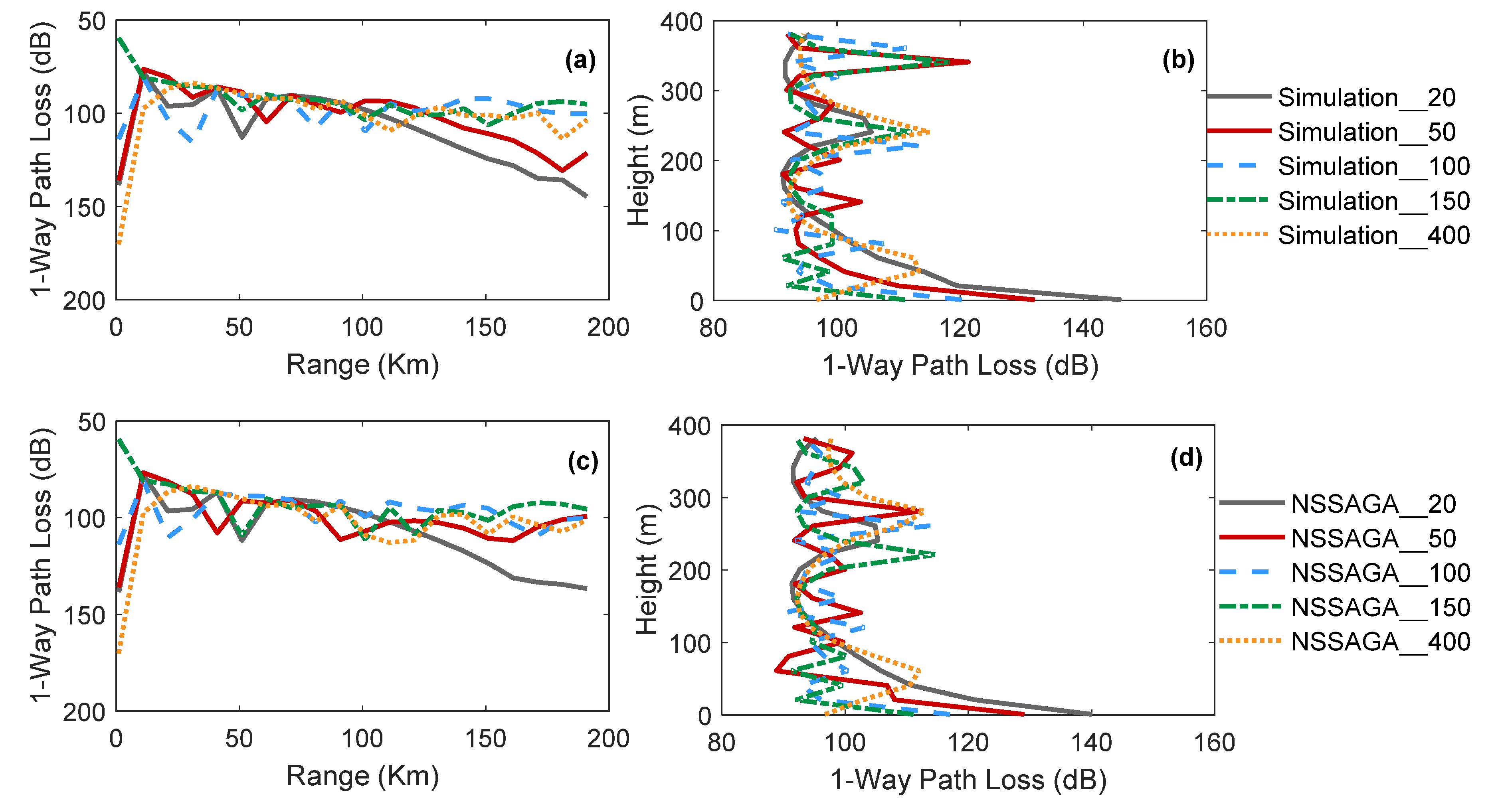
Figure 7a,c depict the propagation loss of the GPS signal over horizontal distances of 0–200 km at a height of 100 m for different antenna heights, showing that the propagation loss decreases with range in each case. Obviously, the overall trend of the propagation loss remains the same for different antenna heights. The amplitude of the propagation loss does not change, but changes in interference pattern alter its position. Those positional changes demonstrate that propagation losses for different antenna heights could be combined to retrieve the refractivity profile more effectively. Based on this feature, we integrated the measurements from different receivers and constructed the Bartlett function to retrieve the atmospheric refractivity structure. Figure 7b,d show how the propagation loss of the GPS signal changes with height at a distance of 100 km. The amplitude of the propagation loss in the duct layer remains around 100 dB, indicating vividly the trapping effect of the surface duct. As Figure 7 shows, the retrieved and simulated propagation losses differ little.

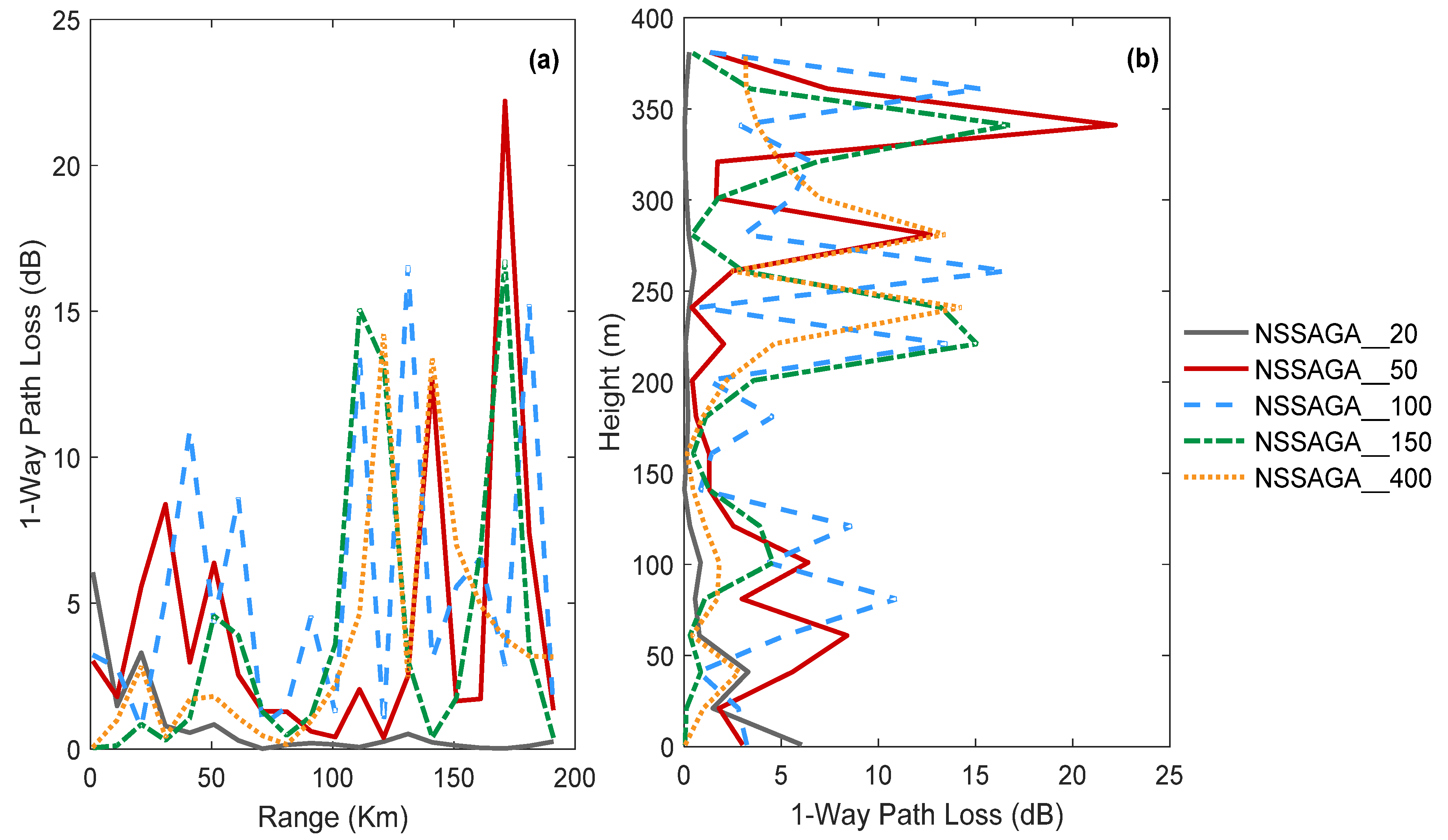
Figure 8 shows the absolute error between the inversion results and the simulated true value. It is found that NSSAGA keeps the absolute error within modest bounds. Because of the model’s defects, a larger error arises beyond 100 km, but the inverted profile can still depict the refractivity environment roughly. Overall, based on the retrieved propagation loss, NSSAGA is highly capable of retrieving the refractivity structure at distances up to 100 km.

4.4. NSSAGA with Different Objective Functions

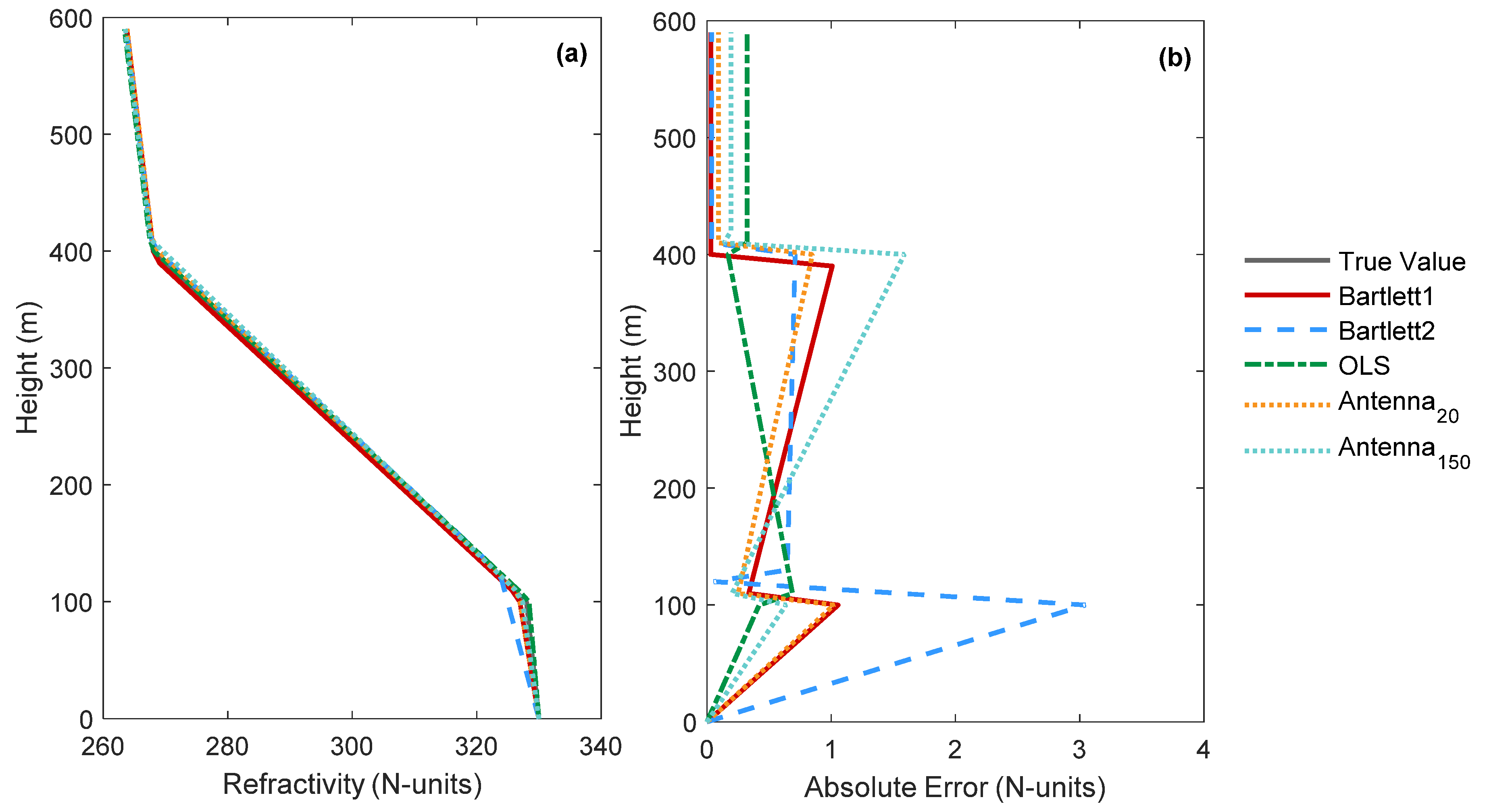
Next, we integrated all the data from antenna of different heights and used them to retrieve the refractivity structure. Figure 9 shows the distinctions among the different objective functions, and the objective functions of Equations (14) and (15) are compared in

Table 3. The value of inversion parameters by NSSAGA with different objective functions (bold font indicates best retrieved parameters).

Objective Function		Inversion Slope c1	Height h1	Inversion Slope c2	Height h2
NSSAGA	Bartlett1	−0.0306 (53%)	104.3187 (4.3%)	−0.2024 (1.2%)	289.7689 (−3.4%)
	Bartlett2	−0.0505 (152.5%)	124.6875 (24.7%)	−0.1998 (−0.1%)	279.5246 (−6.8%)
	OLS	−0.0158 (−21%)	101.5392 (1.5%)	−0.2018 (0.9%)	301.2038 (0.4%)
	20 m	−0.0302 (51%)	107.4749 (7.5%)	−0.1979 (−1.1%)	296.8430 (−1.1%)
	150 m	−0.0264 (32%)	104.6840 (4.7%)	−0.1952 (−2.4%)	305.6387 (1.9%)

. From Table 3, it is easily seen that OLS offers the best performance in retrieving refractivity parameters. However, this good parametric inversion does not mean that the inversion profiles are closer to the true profiles.

Figure 9 illustrates the results obtained with the Bartlett objective function and the least-squares function. Bartlett1 (the red solid line) takes the antenna height information into account, whereas Bartlett2 (the blue dashed line) does not. OLS provides inversion results from all data based on the least-squares method considering the antenna height information. In comparison with Antenna₂₀ and Antenna₁₅₀, Bartlett1 provides fairly good estimates and is even better than Bartlett2. Here, Antenna₂₀ and Antenna₁₅₀ imply the reconstructed results from the received information at 20 m and 150 m. Because the lots of detection information could improve the accuracy of inversion, OLS is expected to perform better than Antenna₂₀ and Antenna₁₅₀. The discrepancy in absolute error between Bartlett1 and OLS is less than 1 N-unit, meaning that Bartlett1 is an acceptable alternative for refractivity inversion.

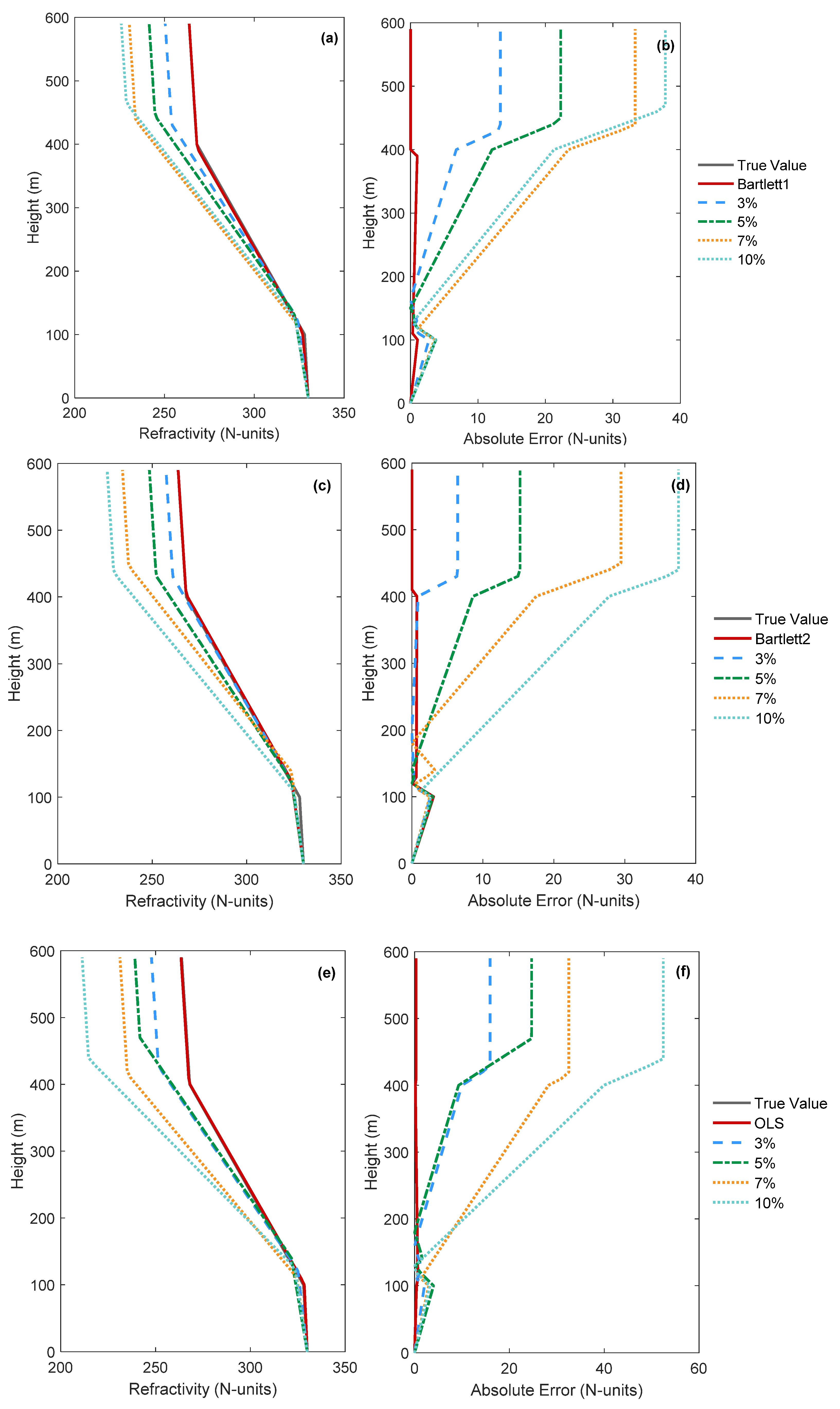
To assess the performance of NSSAGA with three objective functions under different Gaussian noise conditions, the optimal refractivity retrievals are provided in Figure 10 and

Table 4. The value of inversion parameters by NSSAGA with different objective functions and Gaussian noise (bold font indicates best retrieved parameters).

Objective Function and Noise Level		Inversion Slope c1	Height h1	Inversion Slope c2	Height h2
Bartlett1	3%	−0.0476 (138%)	125.2315 (25.2%)	−0.2287 (14.4%)	306.4400 (2.2%)
	5%	−0.0578 (189%)	132.5299 (32.5%)	−0.2484 (24.2%)	312.4563 (4.2%)
	7%	−0.0557 (178.5%)	117.3913 (17.4%)	−0.2791 (39.6%)	321.0724 (7.0%)
	10%	−0.0572 (186%)	125.0450 (25.1%)	−0.2768 (38.4%)	339.8595 (13.3%)
Bartlett2	3%	−0.0461 (130.5%)	119.1744 (19.2%)	−0.2043 (2.2%)	311.4039 (3.8%)
	5%	−0.0497 (148.5%)	123.1673 (23.2%)	−0.2330 (16.5%)	308.2942 (2.8%)
	7%	−0.0453 (126.5%)	138.2198 (38.2%)	−0.2799 (40.0%)	308.1836 (2.7%)
	10%	−0.0470 (135%)	109.1366 (9.1%)	−0.2911 (45.6%)	327.2096 (9.1%)
OLS	3%	−0.0408 (104%)	123.0645 (23.1%)	−0.2418 (20.9%)	304.0172 (1.3%)
	5%	−0.0599 (199.5%)	140.5727 (40.6%)	−0.2423 (21.2%)	329.4880 (9.8%)
	7%	−0.0498 (149%)	111.2574 (11.3%)	−0.2934 (46.7%)	304.5782 (1.5%)
	10%	−0.0523 (161.5%)	125.7983 (25.8%)	−0.3477 (73.9%)	312.7544 (4.3%)

. Using the Bartlett objective function improves the inversion ability of NSSAGA under Gaussian noise conditions, and Bartlett1 is more accurate than Bartlett2 below 100 m. The limited simulations presented herein suggest that Bartlett1 provides better inversion results and has stronger noise immunity for refractivity estimation.

4.5. Experimental Data Testing

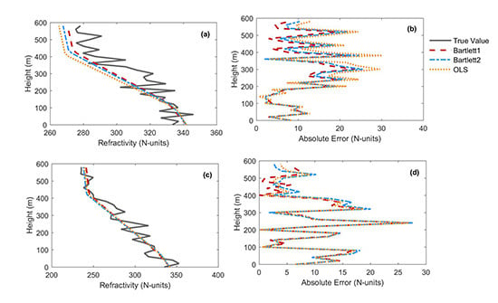
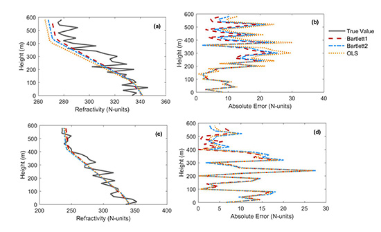
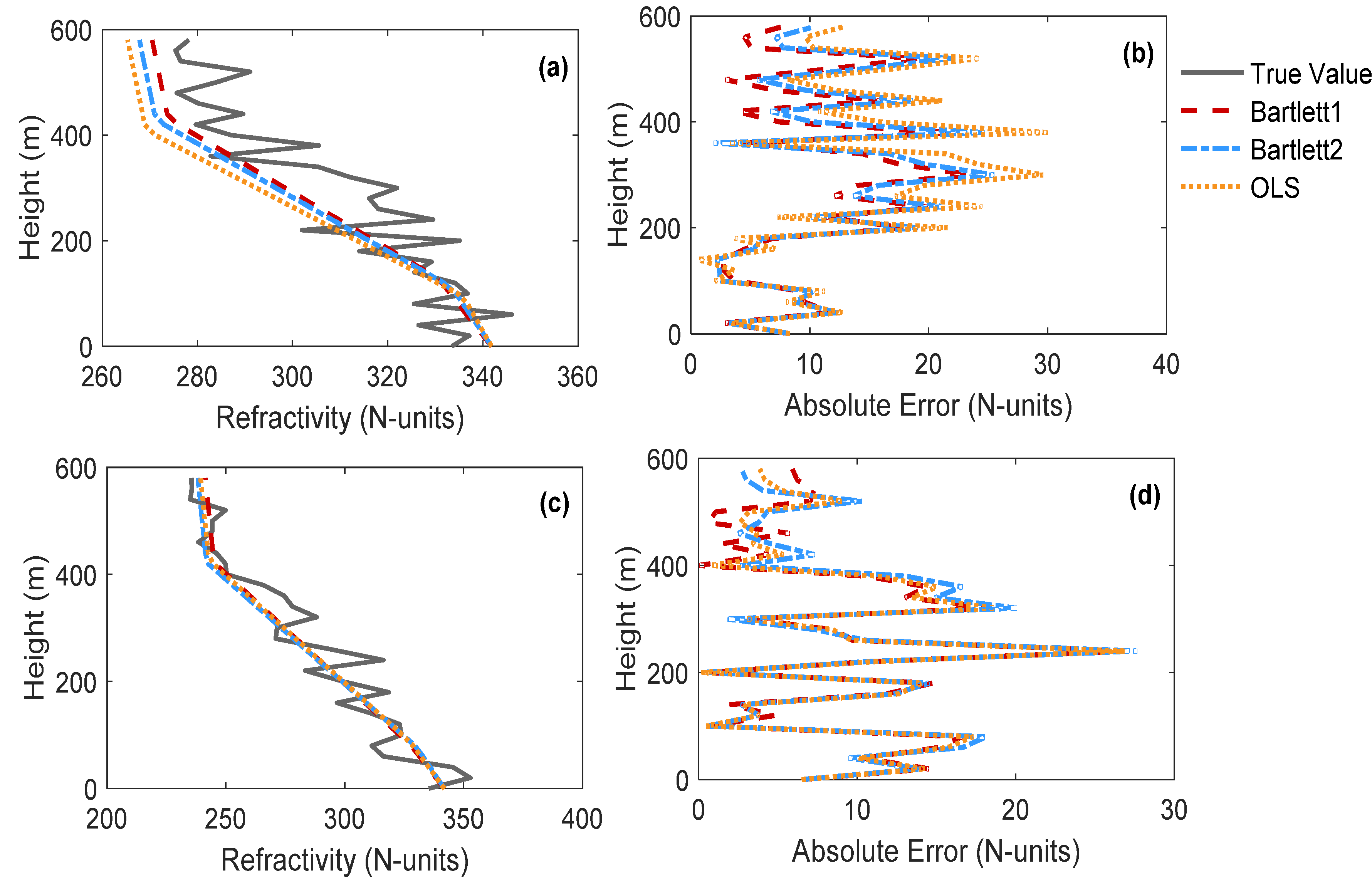
To demonstrate that the NSSAGA can provide sufficient retrieval accuracy under realistic conditions, the excess phase and propagation loss measured by ground-based GPS receiver were used. The excess phase was estimated using a modified version of the Bernese v5.0 software, and the propagation loss was calculated according to the receiving power density of the antenna [35]. Zero-differenced observations were processed in precise point positioning module and the tropospheric zenith delay (phase delay) module produces cleaned post-fit residuals and forms baselines. Finally, slant tropospheric delay was determined through parameter estimation [50]. The corresponding sounding data were obtained from meteorological-rocket detection data (~4 m sampling at altitudes less than 1.5 km) and low-resolution radiosondes (~50 m sampling at altitudes less than 6 km). These experimental data were collected from observations made in the vicinity of Poyang Lake, China (115.27°E, 29.11°N).

Table 5. The value of inversion parameters by different inversion methods.

Parameters		Inversion Slope c1 (N-Units/m)	Height h1 (m)	Inversion Slope c2 (N-Units/m)	Height h2 (m)	RMS Error (N)
Case1	Bartlett1	−0.0746	110.9846	−0.1960	317.8961	11.4734
	Bartlett2	−0.0867	127.4610	−0.1875	303.5692	12.6298
	OLS	−0.0627	94.7159	−0.2120	314.6175	14.3666
Case2	Bartlett1	−0.1689	77.0123	−0.2138	341.3519	8.9907
	Bartlett2	−0.1477	76.1761	−0.2549	351.2348	9.0134
	OLS	−0.1619	87.1056	−0.2513	342.0737	9.2483

gives the inversion parameters obtained using different inversion methods, and Figure 11 shows the differences between the estimated results and the sounding data. Here, only two groups of ground-based GPS data were retrieved (Figure 11a,b: the observed time is 06:17, and Figure 11c,d: the observed time is 18:42).

In Figure 11, the estimated profiles along with the measured profiles are on the left side of the figure. Although the real data contain some observation errors, the estimated profiles are consistent with the measured profiles in general. In these observed cases, Bartlett1 and Bartlett2 provide better fits. However, the absolute error demonstrates that the refractivity profiles estimated using Bartlett1 are much closer to the real refractivity environment than is the case for Bartlett2 or OLS. Also, from the root-mean-square errors of the different inversion methods in the two cases, we conclude that Bartlett1 can be applied to realistic conditions with sufficient retrieval accuracy.

5. Conclusions

A surface duct can substantially affect the performance of radar or communication systems designed according to standard atmospheric conditions. Hence, estimating refractivity profiles plays an important role in predicting the performance of electromagnetic systems [26]. In this paper, based on previous work [35], we put forward an improved retrieval method, using the hybrid NSSAGA algorithm with match-field processing to retrieve tropospheric refractivity profiles. The present study made use of ground-based GPS phase delay and propagation loss from antenna of multiple heights to estimate the surface duct. In the simulations, conventional NSGA-II was chosen to test the performance of NSSAGA under different levels of noise. The presented results demonstrated that NSSAGA is more accurate and that the inverting profiles for the hybrid algorithm are much closer to the simulated profile than those for NSGA-II when using the same objective function. Under Gaussian noise of different levels, the estimated results demonstrated that NSSAGA has strong noise immunity and can be applied to practical situations.

Furthermore, in comparing two objective functions, the match-field processing method gave results that were better than those of the least-squares method in simulations. The refractivity-profile estimates by Bartlett1 under Gaussian noise of different levels were very good, whereas those by other inversion methods were less accurate. The simulations demonstrated that Bartlett1 is an acceptable alternative for refractivity inversion. Actual measurements were also used to test the improved inversion method, and the retrieved results showed that the new method can depict the real refractivity environment. However, the effect of elevation angle on the improved inversion method was not considered herein and will be the subject of future investigations.

References

- Wang, B.; Wu, Z.S.; Zhao, Z.W.; Wang, H.G. A Passive Technique to Monitor Evaporation Duct Height Using Coastal GNSS-R. IEEE Geosci. Remote Sens. 2011, 8, 587–591. [Google Scholar] [CrossRef]
- Sun, Z.; Ning, H.; Song, S.; Yan, D. First observations of elevated ducts associated with intermittent turbulence in the stable boundary layer over Bosten Lake, China. J. Geophys. Res. Atmos. 2016, 121. [Google Scholar] [CrossRef]
- Turton, J.D.; Bennetts, D.A.; Farmer, S.F.G. An introduction to radio ducting. Meteorol. Mag. 1988, 117, 245–254. [Google Scholar]
- Ding, J.; Fei, J.; Huang, X.; Cheng, X.; Hu, X. Observational Occurrence of Tropical Cyclone Ducts from GPS Dropsonde Data. J. Appl. Meteorol. Clim. 2013, 52, 1221–1236. [Google Scholar] [CrossRef]
- Thompson, W.T.; Haack, T. An Investigation of Sea Surface Temperature Influence on Microwave Refractivity: The Wallops-2000 Experiment. J. Appl. Meteorol. Clim. 2011, 50, 2319–2337. [Google Scholar] [CrossRef]
- Atkinson, B.W.; Li, J.-G.; Plant, R.S. Numerical Modeling of the Propagation Environment in the Atmospheric Boundary Layer over the Persian Gulf. J. Appl. Meteorol. 2001, 40, 586–603. [Google Scholar] [CrossRef]
- Haack, T.; Burk, S.D. Summertime Marine Refractivity Conditions along Coastal California. J. Appl. Meteorol. 2001, 40, 673–687. [Google Scholar] [CrossRef]
- Feng, Y.-C.; Fabry, F.; Weckwerth, T.M. Improving Radar Refractivity Retrieval by Considering the Change in the Refractivity Profile and the Varying Altitudes of Ground Targets. J. Atmos. Ocean. Technol. 2016, 33, 989–1004. [Google Scholar] [CrossRef]
- Wagner, M.; Gerstoft, P.; Rogers, T. Estimating refractivity from propagation loss in turbulent media. Radio Sci. 2016, 51. [Google Scholar] [CrossRef]
- Gerstoft, P.; Gingras, D.F.; Rogers, L.T.; Hodgkiss, W.S. Estimation of radio refractivity structure using matched-field array processing. IEEE Trans. Antennas Propag. 2000, 48, 345–356. [Google Scholar] [CrossRef]
- Zeng, Y.; Blahak, U.; Neuper, M.; Jerger, D. Radar Beam Tracing Methods Based on Atmospheric Refractive Index. J. Atmos. Ocean. Technol. 2014, 31, 2650–2670. [Google Scholar] [CrossRef]
- Shume, E.; Ao, C. Remote sensing of tropospheric turbulence using GPS radio occultation. Atmos. Meas. Tech. 2016, 9, 3175–3182. [Google Scholar] [CrossRef]
- Fountoulakis, V.; Earls, C. Duct heights inferred from radar sea clutter using proper orthogonal bases. Radio Sci. 2016, 51. [Google Scholar] [CrossRef]
- Hallali, R.; Dalaudier, F.; Parent du Chatelet, J. Comparison between Radar and Automatic Weather Station Refractivity Variability. Bound.-Layer Meteorol. 2016, 160, 299–317. [Google Scholar] [CrossRef]
- Krolik, J.; Tabrikian, J. Tropospheric refractivity estimation using radar clutter from the sea surface. In Proceedings of the Battlespace Atmospheric Conference, San Diego, CA, USA, 2–4 December 1997. [Google Scholar]
- Gerstoft, P.; Rogers, L.T.; Hodgkiss, W.S.; Wagner, L.J. Refractivity estimation using multiple elevation angles. IEEE J. Ocean. Eng. 2003, 28, 513–525. [Google Scholar] [CrossRef]
- Gerstoft, P.; Rogers, L.T.; Krolik, J.L.; Hodgkiss, W.S. Inversion for refractivity parameters from radar sea clutter. Radio Sci. 2003, 38. [Google Scholar] [CrossRef]
- Sheng, Z. The estimation of lower refractivity uncertainty from radar sea clutter using the Bayesian—MCMC method. Chin. Phys. B 2013, 22. [Google Scholar] [CrossRef]
- Douvenot, R.; Fabbro, V.; Gerstoft, P.; Bourlier, C.; Saillard, J. A duct mapping method using least squares support vector machines. Radio Sci. 2008, 43. [Google Scholar] [CrossRef] [Green Version]
- Yardim, C.; Gerstoft, P.; Hodgkiss, W.S. Tracking Refractivity from Clutter Using Kalman and Particle Filters. IEEE Trans. Antennas Propag. 2008, 56, 1058–1070. [Google Scholar] [CrossRef]
- Wen, D.; Yuan, Y.; Ou, J.; Zhang, K. Ionospheric Response to the Geomagnetic Storm on August 21, 2003 over China Using GNSS-Based Tomographic Technique. IEEE Trans. Geosci. Remote Sens. 2010, 48, 3212–3217. [Google Scholar] [CrossRef]
- Sheng, Z.; Wang, J.; Zhou, S.; Zhou, B. Parameter estimation for chaotic systems using a hybrid adaptive cuckoo search with simulated annealing algorithm. Chaos 2014, 24. [Google Scholar] [CrossRef] [PubMed]
- Zhao, X.; Huang, S. Atmospheric Duct Estimation Using Radar Sea Clutter Returns by the Adjoint Method with Regularization Technique. J. Atmos. Ocean. Technol. 2014, 31, 1250–1262. [Google Scholar] [CrossRef]
- Karimian, A.; Yardim, C.; Gerstoft, P.; Hodgkiss, W.S.; Barrios, A.E. Refractivity estimation from sea clutter: An invited review. Radio Sci. 2011, 46. [Google Scholar] [CrossRef]
- Zhao, X.; Yardim, C.; Wang, D.; Howe, B.M. Estimating range-dependent evaporation duct height. J. Atmos. Ocean. Technol. 2017, 34, 1113–1123. [Google Scholar] [CrossRef]
- Zhang, J.; Wu, Z.; Wang, B.; Wang, H.; Zhu, Q. Modeling low elevation GPS signal propagation in maritime atmospheric ducts. J. Atmos. Sol.-Terr. Phys. 2012, 80, 12–20. [Google Scholar] [CrossRef]
- Hitney, H.V. Remote sensing of refractivity structure by direct radio measurements at UHF. In AGARD, Remote Sensing of the Propagation Environment 6 p; (SEE N92-22790 13-46); Naval Ocean Systems Center: San Diego, CA, USA, 1992. [Google Scholar]
- Anderson, K.D. Tropospheric refractivity profiles inferred from low elevation angle measurements of Global Positioning System (GPS) signals. In Proceedings of the AGARD Conference the Sensor and Propagation Panel Symposium, Bremerhaven, Germany, 19–22 September 1994. [Google Scholar]
- Lowry, A.R.; Rocken, C.; Sokolovskiy, S.V.; Anderson, K.D. Vertical profiling of atmospheric refractivity from ground-based GPS. Radio Sci. 2002, 37. [Google Scholar] [CrossRef]
- Lin, L.K.; Zhao, Z.W.; Zhang, Y.R.; Zhu, Q.L. Tropospheric refractivity profiling based on refractivity profile model using single ground-based global positioning system. IET Radar Sonar Navig. 2011, 5, 7–11. [Google Scholar] [CrossRef]
- Zus, F.; Dick, G.; Heise, S.; Wickert, J. A forward operator and its adjoint for GPS slant total delays. Radio Sci. 2015, 50, 393–405. [Google Scholar] [CrossRef]
- Sheng, Z.; Fang, H.-X. Monitoring of ducting by using a ground-based GPS receiver. Chin. Phys. B 2013, 22. [Google Scholar] [CrossRef]
- Wu, X.; Wang, X.; Lü, D. Retrieval of vertical distribution of tropospheric refractivity through ground-based GPS observation. Adv. Atmos. Sci. 2014, 31. [Google Scholar] [CrossRef]
- Wu, Y.-Y.; Hong, Z.-J.; Guo, P.; Zheng, J. Simulation of Atmospheric Refractive Profile Retrieving from Low-Elevation Ground-Based GPS Observations. Chin. J. Geophys. 2010, 53, 639–645. [Google Scholar] [CrossRef]
- Liao, Q.; Sheng, Z.; Shi, H. Joint Inversion of Atmospheric Refractivity Profile Based on Ground-Based GPS Phase Delay and Propagation Loss. Atmosphere 2016, 7, 12. [Google Scholar] [CrossRef]
- Gingras, D.F.; Gerstoft, P.; Gerr, N.L. Electromagnetic matched-field processing: Basic concepts and tropospheric simulations. IEEE Trans. Antennas Propag. 1997, 45, 1536–1545. [Google Scholar] [CrossRef]
- Smith, E.K.; Weintraub, S. The Constants in the Equation for Atmospheric Refractive Index at Radio Frequencies. Proc. IRE 1953, 41, 1035–1037. [Google Scholar] [CrossRef]
- Zhao, X.; Huang, S.; Xiang, J.; Shi, W.L. Remote sensing of atmospheric duct parameters using simulated annealing. Chin. Phys. B 2011, 9. [Google Scholar] [CrossRef]
- Almond, T.; Clarke, J. Considerations of the usefulness of the microwave prediction methods on air-to-ground paths. IEEE Proc. Part F 1973, 130, 649–656. [Google Scholar] [CrossRef]
- Levy, M.F. Horizontal parabolic equation solution of radiowave propagation problems on large domains. IEEE Trans. Antennas Propag. 1995, 43, 137–144. [Google Scholar] [CrossRef]
- Teti, J. Parabolic equation methods for electromagnetic wave propagation [Book Review]. IEEE Antennnas Propag. Mag. 2001, 43, 96–97. [Google Scholar] [CrossRef]
- Balvedi, G.C.; Walter, F. Analysis of GPS signal propagation in tropospheric ducts using numerical methods. In Proceedings of the 11th URSI Commission Open Symposium on Radio Wave Propagation and Remote Sensing, Rio De Janeiro, Brazil, 30 October–2 November 2007. [Google Scholar]
- Deb, K.; Pratap, A.; Agarwal, S.; Meyarivan, T. A fast and elitist multiobjective genetic algorithm: NSGA-II. IEEE Trans. Evolut. Comput. 2002, 6, 182–197. [Google Scholar] [CrossRef]
- Li, H.; Zhang, Q. Multiobjective Optimization Problems with Complicated Pareto Sets, MOEA/D and NSGA-II. IEEE Trans. Evolut. Comput. 2009, 13, 284–302. [Google Scholar] [CrossRef]
- Metropolis, N.; Rosenbluth, A.W.; Rosenbluth, M.N.; Teller, A.H.; Teller, E. Equation of state calculations by fast computing machines. J. Chem. Phys. 1953, 21, 1087–1092. [Google Scholar] [CrossRef]
- Srinivas, N.; Deb, K. Multiobjective function optimization using nondominated sorting genetic algorithms. Evol. Comput. 1994, 2, 221–248. [Google Scholar] [CrossRef]
- Xiang, Y.; Gubian, S.; Suomela, B.; Hoeng, J. Generalized simulated annealing for global optimization: The GenSA Package. R J. 2013, 5, 13–29. [Google Scholar]
- Rogers, L.T. Likelihood estimation of tropospheric duct parameters from horizontal propagation measurements. Radio Sci. 1997, 32, 79–92. [Google Scholar] [CrossRef]
- Zus, F.; Bender, M.; Deng, Z.; Dick, G.; Heise, S.; Shang-Guan, M.; Wickert, J. A methodology to compute GPS slant total delays in a numerical weather model. Radio Sci. 2012, 47. [Google Scholar] [CrossRef] [Green Version]
- Kačmařík, M.; Douša, J.; Dick, G.; Zus, F.; Brenot, H.; Möller, G.; Pottiaux, E.; Kapłon, J.; Hordyniec, P.; Václavovic, P.; et al. Inter-technique validation of tropospheric slant total delays. Atmos. Meas. Tech. 2017, 10, 2183–2208. [Google Scholar] [CrossRef]
Figure 1.
Geometry of ground-based Global Positioning System (GPS) occultation for computing phase-delay.
Figure 2.
Flow-chart of non-dominated sorting and simulated annealing genetic algorithm (NSSAGA) algorithm.
Figure 3.
Geometric scheme of refractivity profile model.
Figure 4.
Flowchart of calculating objective value. (a) Consider the effect of antenna height. (b) Neglect the effect of antenna height.
Figure 5.
Retrieved refractivity profiles and corresponding absolute error by using (a,b) NSSAGA and (c,d) non-dominated sorting genetic algorithm II (NSGA-II) with antenna heights of 20 m, 100 m, 150 m, and 400 m.
Figure 6.
The retrieved refractivity profile and corresponding absolute error by NSSAGA under different Gaussian Noise levels. Antenna heights used are (a,b) 20 m; (c,d) 50 m; (e,f) 100 m; (g,h) 150 m; (i,j) 400 m.
Figure 7.
The propagation loss of ground-based GPS signal. (a,c) Simulation and inversion results at distance of 0–200 km and height of 100 m; (b,d) simulation and inversion results at distance of 100 km and height of 0–400 m.
Figure 8.
The absolute error of propagation loss. (a) Distance of 0–200 km and height of 100 m and (b) distance of 100 km and height of 0–400 m.
Figure 9.
Comparison of retrieved refractivity profile and absolute error by NSSAGA with various objective functions.
Figure 10.
The retrieved refractivity profile and corresponding absolute error by NSSAGA with different objective functions. (a,b) The Bartlett objective function with the receiver height information; (c,d) the Bartlett objective function without the receiver height information; (e,f) the least-squares method with the receiver height information.
Figure 11.
Refractivity profiles by different inversion methods for real atmospheric environment. (a,b): time for Case 1 is 06:17; (c,d): time for Case 2 is 18:42.