Article

Topographic Correction of Forest Image Data Based on the Canopy Reflectance Model for Sloping Terrains in Multiple Forward Mode

1
State Key Laboratory of Subtropical Silviculture, Zhejiang A & F University, Lin’an 311300, China
2
Key Laboratory of Carbon Cycling in Forest Ecosystems and Carbon Sequestration of Zhejiang Province, Zhejiang A & F University, Lin’an 311300, China
3
School of Environmental and Resources Science, Zhejiang A & F University, Lin’an 311300, China
4
State Key Laboratory of Remote Sensing Science, Institute of Remote Sensing and Digital Earth, Chinese Academy of Sciences, Beijing 100101, China
5
Research Center for Digital Mountain and Remote Sensing Application, Institute of Mountain Hazards and Environment, Chinese Academy of Sciences, Chengdu 610041, China
6
International Institute for Earth System Science, Nanjing University, Nanjing 210046, China
7
Department of Global Ecology, Carnegie Institution for Science, Stanford, CA 94305, USA
*
Authors to whom correspondence should be addressed.
Remote Sens. 2018, 10(5), 717; https://doi.org/10.3390/rs10050717
Submission received: 21 March 2018 / Revised: 26 April 2018 / Accepted: 5 May 2018 / Published: 7 May 2018
(This article belongs to the Section Forest Remote Sensing)

Abstract

:
Topographic correction methods rarely consider the canopy parameter effects directly and explicitly for sloping canopies. In order to address this problem, the topographic correction method MFM-GOST2 was developed by implementing the second version of the Geometric-Optical model for Sloping Terrains (the GOST2 model) in the multiple forward mode (MFM) inversion framework. First, a look up table (LUT) was constructed by multiple forward modeling of the GOST2 model; second, the radiance of a remotely sensed image and its corresponding topographic data were used for searching potential canopy parameter combinations from the LUT; and third, the corrected radiance was determined by averaging potential radiances of horizontal canopies from the LUT according to the canopy parameter combinations. The MFM-GOST2 and twelve generally used topographic correction methods were evaluated via a case study by visual analysis, linear relationship analysis, and the rose diagram analysis. The result showed that the MFM-GOST2 method successfully removed most of the topographic effects of a subset image of the Landsat-8 image in a case study. The case study also illustrates that the rose diagram analysis is a good way to evaluate topographic corrections, but the linear relationship analysis cannot be used independently for the evaluations because the decorrelation is not a sufficient condition to determine a successful topographic correction.

1. Introduction

Over the past decades, topographic relief has greatly limited remote sensing applications, such as ground-objects identification, land cover classification, and forest biophysical parameters estimation [1,2]. In order to remove topographic effects in remotely sensed images, various topographic correction methods have been developed and implemented [3]. Forest canopy is one of the most common land cover types on earth. Although the variation of spectral radiances caused by the varying canopy structures has been recognized since the 1990s [4,5], the detailed canopy structure has not been fully considered by most topographic correction methods [3,6].
The early studies regarding topographic correction methods were summarized by Soenen et al. [3], Chander et al. [7], Hantson and Chuvieco [8], and Vanonckelen et al. [6]. These methods can be grouped as photometric and empirical methods, sun-canopy-sensor methods, and physically based methods (listed in Table 1, [3]).
One of the most generally photometric and empirical corrections is the COSIN-T correction (Cosin correction, [9]), which is developed based on Lambert’s cosine law. This model is easily applicable because only solar and slope angles are required [19]. Due solely to the simplicity of the method, the effect of diffuse illumination is not accounted for, resulting in overestimation of the output radiance data, and in some cases, large errors [3]. Several studies have indicated that this method also tends to overcorrect in areas under low illumination conditions [8,9,20]. In order to compensate for the overcorrection by COSIN-T, the COSIN-C correction is developed by Civco [10]. COSIN-C is more appropriate for rugged terrain since they included moderators to the COSIN-T correction that improved the effectiveness of corrections over steep and shaded slopes [3,21,22]. The C correction [9] is another modified form of the COSIN-T correction and introduces an empirical parameter c , accounting for the contribution of indirect irradiance to the incident solar flux over slopes [23]. However, the Lambertian framework of the COSIN-T, COSIN-C, and C corrections has been shown, both theoretically and empirically, to be inappropriate in forested terrain [3,11,12,22]. For the purpose of overcoming the shortcomings of the Lambertian surface assumption, Smith et al. [13] introduced an empirical parameter k (between 0 and 1) to qualify the level of anisotropic scattering over a non-Lambertian surface and developed the Minnaert correction [23]. In this method, it is assumed that the surfaces behave in a perfectly Lambertian manner when the Minnaert constant k is 1, and then the method is degraded to the COSIN-T correction. Pimple et al. [19] and Hantson and Chuvieco [8] indicated that the application of the C correction and the Minnaert correction over large areas with different land cover types creates problems, resulting from specific Land Use- and Land Cover (LULC)-dependent c and k parameters, respectively. Then, the PBM (Pixel-based Minnaert, Lu et al. [16]) and PBC (Pixel-based C, [17]) corrections were developed for improving the C and Minnaert corrections, respectively. For example, the PBC correction consists of the topographic part of the integrated radiometric correction by Kobayashi and Sanga-Ngoie [17] and implements a factor C λ to account for diffuse sky irradiance [6]. Other methods, depending on empirical equations based on the linear relationship between image data and the angle of incidence, were also categorized as the photometric and empirical method, such as the VECA (Variable Empirical Coefficient Algorithm, [18]) correction and the Teillet regression correction [9]. Both of them are LULC specific [19,24].
Photometric and empirical methods are based on sun-terrain-sensor (STS) geometry [23]; however, in forest stands, this does not properly characterize the sun-canopy-sensor geometry since trees on slopes are not normal to the surface [3,11,12,22]. Based on sun-canopy-sensor geometry, Gu and Gillespie [11] proposed the SCS (Sun-Canopy-Sensor) correction. Gao and Zhang [23] indicated that this method is more appropriate for topographic effect removal over structured forests surfaces. However, Soenen et al. [12] pointed out that the SCS method may significantly overcorrect the topography-induced effects at solar incidence angles approaching 90°. Then, Soenen et al. [12] introduced the empirical parameter c of the C correction into the SCS correction to moderate the effect of diffuse sky illumination, called the SCS + C correction. The empirical parameter k of the Minnaert correction was also introduced into the SCS correction in a similar way to the so-called Minnaert-SCS (Minnaert + Sun-Canopy-Sensor correction, [14]) to overcome the shortcomings of the Lambertian surface assumption of the SCS correction.
The first physically based correction is the Dymond–Shepherd correction [15], which is derived from a simple physical model of canopy reflectance. Four strict assumptions of the method greatly limit its application over sloping canopies: the model requires the vegetation canopy to be deep, the incoming radiation to be primarily direct light, the leaves to be approximately randomly oriented, and the canopy roughness to be invariant with slope. Soenen et al. [3] developed another topographic correction method based on a canopy reflectance model in multiple forward mode called MFM-TOPO. The basic principle of MFM-TOPO is to estimate canopy reflectance over horizontal background from a look-up table (LUT) according to remotely sensed observations over slopes. The superiority of MFM-TOPO is the theoretical possibility to consider the physical process of radiative transfer within a canopy. For this reason alone, the quality of corrected reflectances is determined by the performance of the kernel canopy reflectance model and its corresponding LUT construction process. Soenen et al. [3] emphasized that the LUT of MFM-TOPO was constructed by multiple forward running of the Li–Strahler geometric-optical model (GOMS) [4]. However, the GOMS model is developed for considering the effect of crown shape and mutual shadowing within a canopy, but not for topography. As a matter of fact, GOMS extended for modeling reflectance over sloping terrains is the Schaaf’s model by Schaaf et al. [25]. Although it is unclear how the non-topographic considered GOMS model was used as the core of MFM-TOPO to model the reflectance over slopes by Soenen et al. [3], it still provides a good idea for correcting topographic effects of reflected signals from sloping forests. For this reason, the MFM-TOPO correction was not compared with other correction methods listed in Table 1 in this study.
In this study, we developed the MFM-GOST2 method to correct the topographic effect on remotely sensed radiances based on the MFM inversion framework by implementing the second version of the Geometric-Optical model for Sloping Terrains (GOST2) [26], which considers a detailed description of canopy structures and scattering radiation within a canopy. Then, the reliability of MFM-GOST2 compared with twelve generally used topographic correction methods listed in Table 1, was evaluated by visual analysis, linear relationship analysis, and the rose diagram analysis.

2. Methodology

2.1. The MFM-GOST2 Correction

GOST is a geometric-optical (GO) model for sloping terrains based on the four-scale GO model, which simulates the bidirectional reflectance distribution function (BRDF) of forest canopies on flat surfaces [5,27]. The GOST model considers four scales of sloping canopy architecture: tree groups, tree crowns, branches, and shoots. It considers the fact that trees grow vertically rather than perpendicularly to sloping grounds. The multiple scattering scheme within a sloping canopy can also be simulated using the radiative transfer code of the GOST model [28]. Then, a hybrid canopy reflectance model GOST2 based on GOST is developed with a “ray tracing + GO” method to relax the computational restriction in modeling the area ratios of the sunlit and shaded foliage [26]. In this way, reflectance of sloping canopies can be simulated by GOST2 with given canopy parameters, topographic parameters, and sun-canopy-sensor geometry (Table 2).
Using the GOST2 model as the basis for topographic correction, the three stages described below should be conducted (Figure 1). First, a LUT should be created by multiple forward modeling of GOST2. There were more than 8.6675 × 10¹³ records simulated by GOST2 where user-defined ranges of the input parameters were derived by a set increment in this study. The ranges and increment sizes were set with no a priori information, but were typically defined based on the reality of natural forests [3,29]. In total, 75 uniformly distributed view zenith/azimuth angular combinations and 97 uniformly distributed solar zenith/azimuth angular combinations over hemisphere were used for the LUT construction. The simulated reflectances by GOST2 were then converted to radiances according to Vicente-Serrano et al. [30]:
L λ = R λ E S U N λ cos θ s π d 2
where L λ is the satellite radiance in W·M−2·SR−1·μM−1 for band λ , R λ is the simulated reflectance for band λ , E S U N λ is the mean solar exoatmospheric irradiance for band λ , θ s is the solar zenith angle in degrees, and d is the earth–sun distance in astronomical units. Second, one or more canopy parameter combinations (see Table 2) were determined from the LUT according to given radiances of remotely sensed image, topographic parameters and sun-canopy-sensor geometry. At least one canopy parameter combination can be found from the LUT because a given radiance is mandatory to match the closest simulated radiance in the LUT when no simulated radiance is strictly equal to the observed radiance. Third, the canopy parameter combinations determined in the second step and horizontal assumption (both slope and aspect of background were 0) were used for matching corrected radiances through the LUT again. If the corrected radiances are not unique, the final result was determined by the mean value of the potential simulated radiances.

2.2. Evaluation Methods

Topographic corrections cannot be validated directly because it is impossible to collect ground truth. The generally used methods for evaluating topographic corrections are (1) visual analysis [2]; (2) statistical analysis of the linear relationship between radiances and cosine of incidence angles [31], and (3) classification analysis [19,32]. The former two methods are immediate evaluations and are adopted in this study. As the indirect evaluation method, classification analysis is affected by many kinds of overlapping factors, such as within class covariance of a land cover type. In order to evaluate the topographic correction methods with as few extraneous factors as possible, classification analysis is not adopted in this study. Instead, another statistical analysis called the rose diagram analysis is adopted for evaluations. As for the rose diagram analysis, radiances of a remotely sensed image were divided into three groups according to the fixed slope intervals of canopy backgrounds (0°–20°, 21°–40° and ≥41°). For each group, radiances were divided into 36 sub-groups in 10° aspect angle intervals. Then, mean values of the radiances of the 108 (3 × 36) sub-groups were calculated and plotted in the rose diagram analysis. The polar angle of the rose diagram represents the aspect of background (°), and the radius represents the value of radiances (W/(m2·sr·μm)). If the corrected radiances show no azimuth dependence, the topographic correction can be considered to be successful.

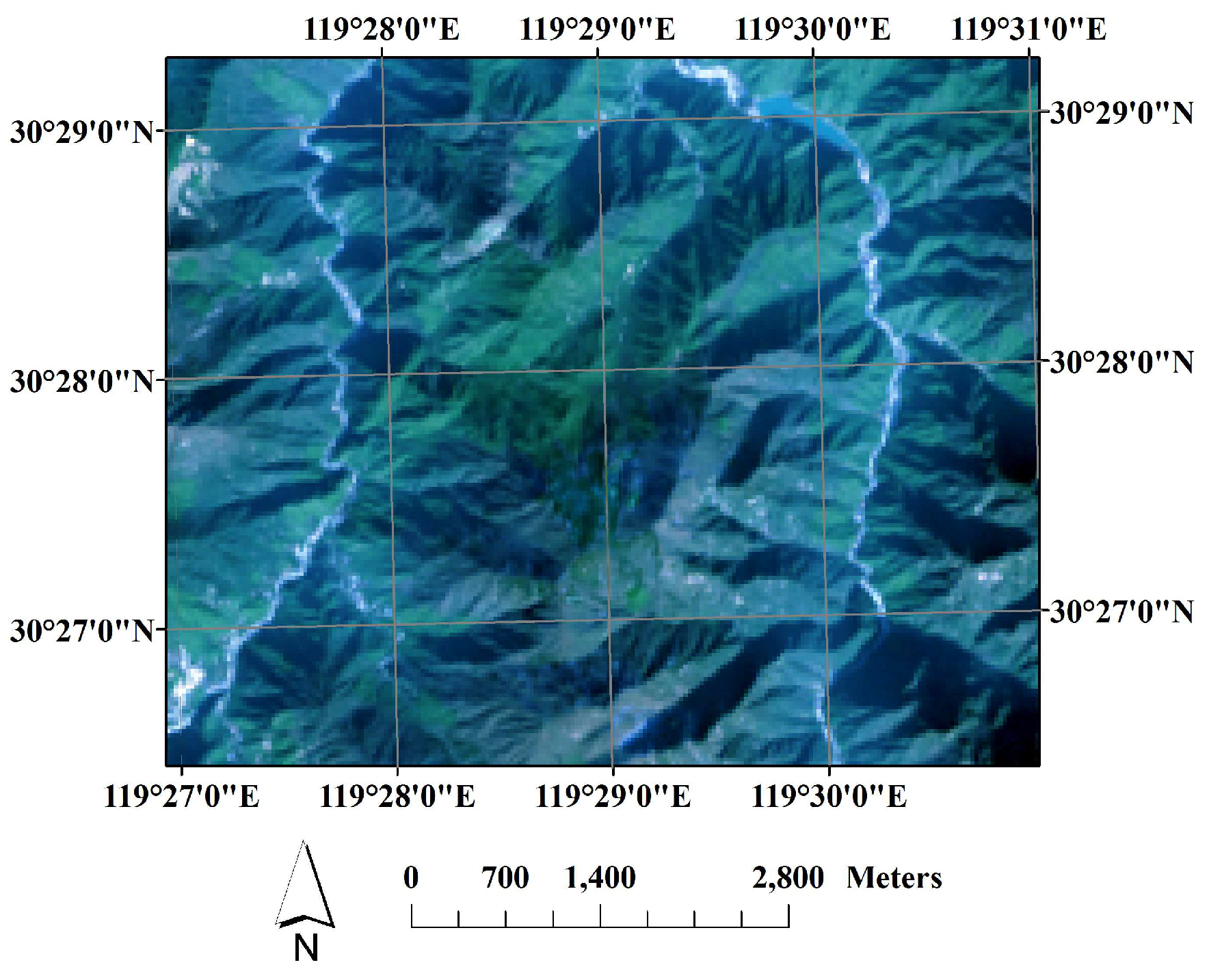
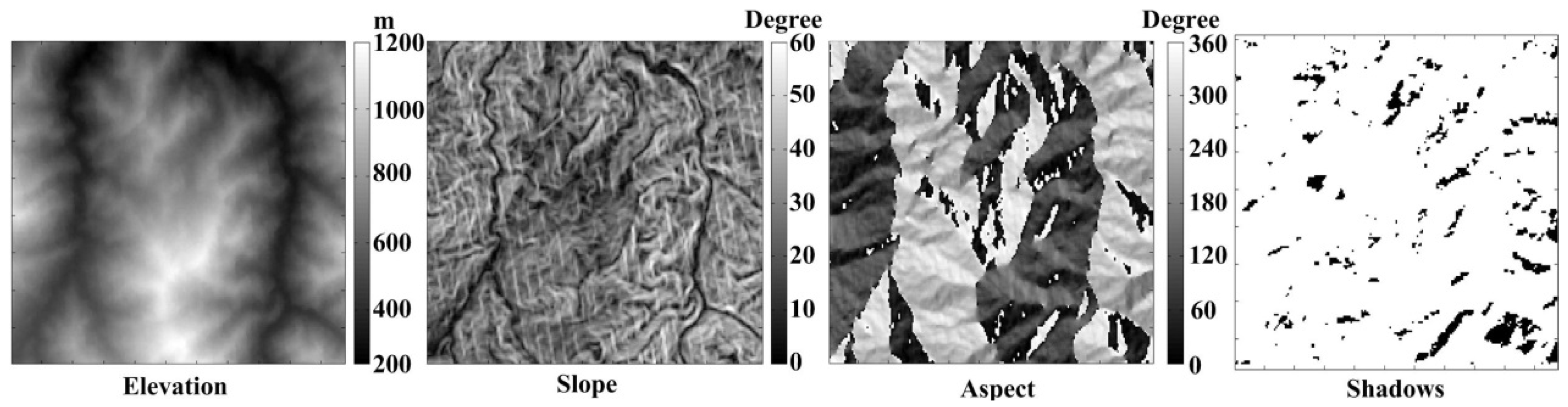
3. Experimental Data

The study area is located in the north of Anji County, Zhejiang, China (Figure 2). The area covers approximately 34 km2 and includes a full range of terrain aspects, and slopes ranging from 0° to 60°. Stand height ranged from 180 m to 1200 m (Figure 3). The vast majority of forest canopies are the planted moso bamboo forest in the study area. Typical measured stem density for this area ranged from 1700 stems/ha to 5600 stems/ha. The growth difference of the bamboo canopies is because of different forest management techniques. The stem densities have no significant difference between sunny and shady slopes due to artificial cultivation. With the increase of slope gradient, the stem density of bamboo canopies shows a gentle decrease. A few scattered trees are distributed within the planted moso bamboo forest, such as Pinus massoniana L., Cunninghamia lanceolata L., Cyclobalanopsis glauca, Castanopsis sclerophylla, Castanopsis eyrei, Schima superba, and Quercus fabri Hance. There are also a few rivers and roads distributed among the bamboo forests.
A subset of the Landsat-8 image (path 119/row 39, 173 × 215 pixels, with 30 m spatial resolution) of the study area is used for the case study. The image subset of the study area is cloud free. The solar zenith and azimuth angles are 57° and 157° on the imaging day of 13 December 2014, respectively. The red (662 nm), near infrared (NIR; 868 nm) and short-wave infrared (SWIR; 1650 nm) bands of the Landsat-8 image are used for the corrections. Then, the original DN (digital number) values of the remotely sensed image were converted into radiances [6]:
L λ = D N × g a i n + o f f s e t
where gain and offset values are obtained from the calibration file in the metadata for each band. In this study, only a 0° view zenith angle is used for the LUT searching process to match the view geometry of the Landsat-8 image. Then, the calibrated radiance values of L λ are atmospherically corrected by the dark object subtraction (DOS) correction [33] which calculates a minimum radiance value (Lp, in W/(m2·sr·μm)) for each band as the 1st percentile radiance values over the image. Lp accounts for the atmospheric effect. Finally, the Lp value is subtracted from all pixels. The Lp value of the red, NIR, and SWIR bands for the entire image are 11.50, 7.01, and 0.56, respectively.
The slope and aspect images are derived from a sub-scene of the National Aeronautics and Space Administration (NASA) SRTM 30 m × 30 m high-resolution digital elevation model (DEM) which is obtained from the U.S. Geological Survey (USGS) and resampled using a nearest neighborhood transformation [34] (Figure 3). According to the sun-canopy-sensor geometry of this case, the canopies which do not receive direct solar radiation are identified as “Shadows” (Figure 3). The “Shadows” pixels are assigned as 0 values because this type of canopies are not theoretically considered by most of the topographic correction methods as mentioned in this study.

4. Results and Analysis

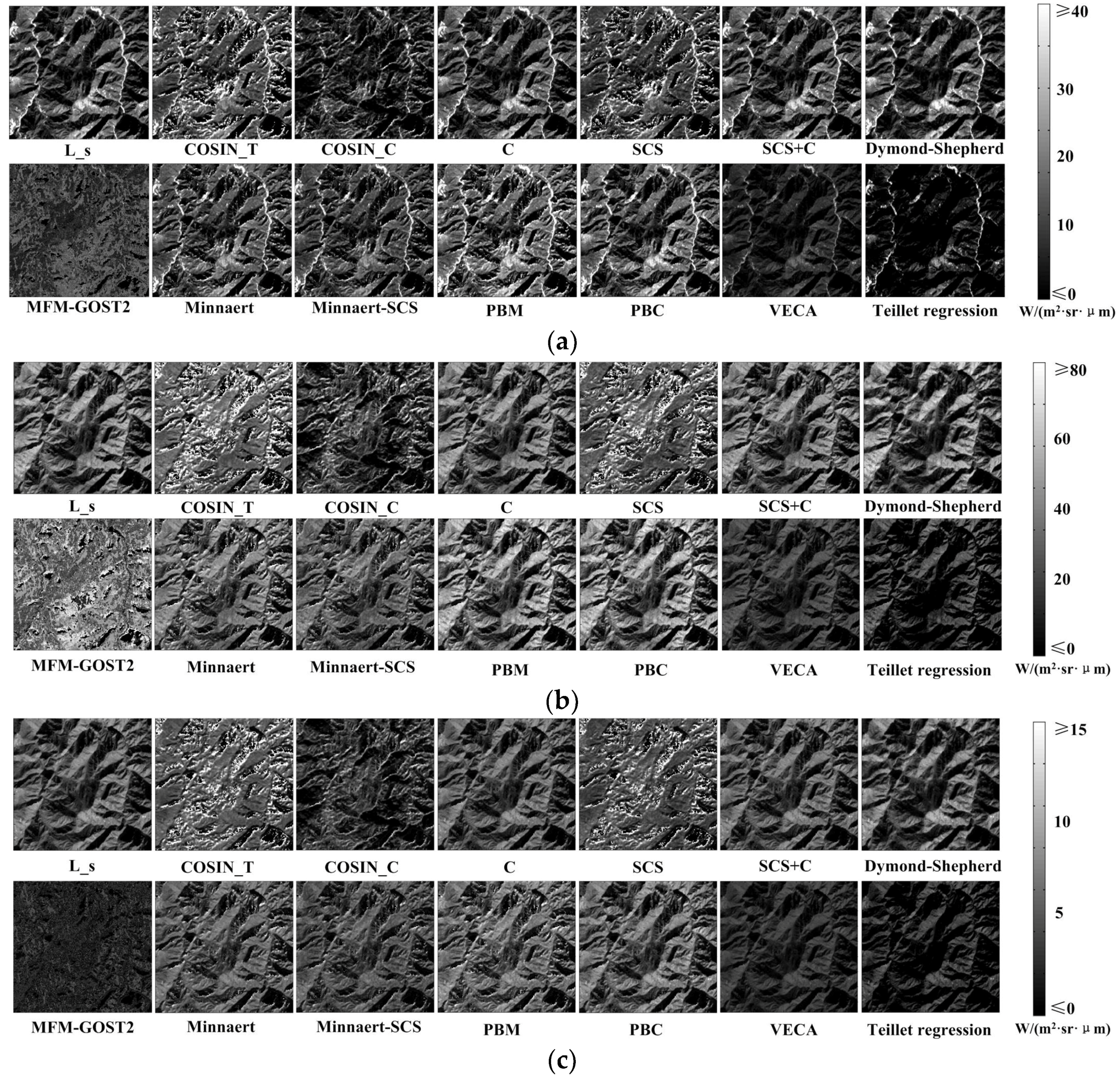
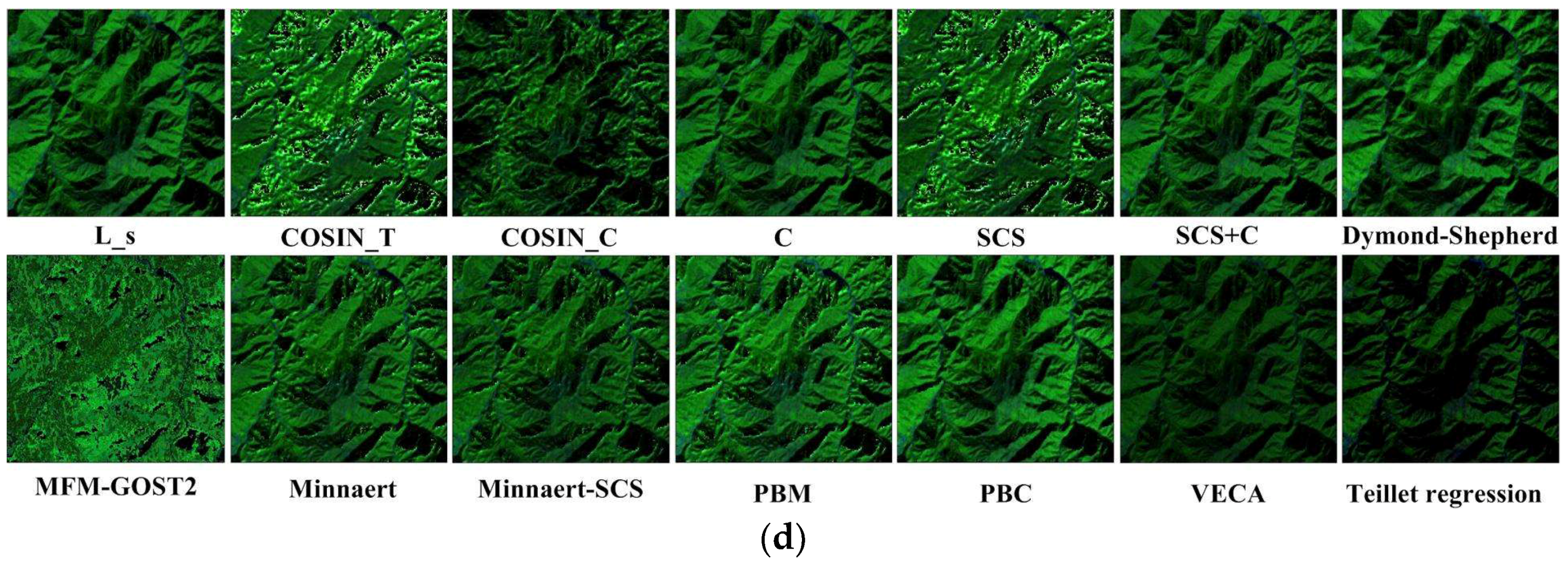
4.1. Visual Analysis

Figure 4 shows the remotely sensed images before and after topographic corrections. Both the gray-scaled and false color composite images (bands 6-5-4 of Landsat-8 OLI) of the study area are presented. The “Shadows” areas show black (the value of radiance is set to 0) in all these corrected images.
Comparing with the uncorrected images, topographic relief effects rarely remained on the corrected images after the MFM-GOST2 correction. It has been revealed that the MFM-GOST2 correction has potential to succeed as expected. The COSIN_T and SCS corrections show the similar overcorrected radiances for shaded canopy slopes. The same as the results by Richter et al. [35] and Ghasemi et al. [36], the overestimation is because of the small cos ( i ) when the incident angle of sunlight is large for steep slopes of shaded canopies. The corrected images by COSIN_C appear to be underestimated in both sunny and shady slopes in visual analysis. It is because the large number of steep slopes leads to small cos ( i ) ¯ . In this study, COSIN_C does not show good improvement on COSIN_T as expected. The VECA and Teillet regression corrections also show underestimations in all the three bands. We found that the reason of the underestimation is because of the small L ¯ values of the uncorrected images. The topographic corrections by C-correction, PBC and SCS + C are not obvious in visual analysis. In this study area, c and C λ values are large because the uncorrected radiance values vary significantly with a large range of incident angle of sunlight. Therefore, the corrected results are controlled by c and C λ values of the three methods, respectively, and then it is easy to infer the small difference before and after the corrections. The corrections by Minnaert and PBM show little improvement in all three bands using the Minnaert constant k λ for considering the non-Lambertian canopy surfaces. The Minnaert-SCS corrections greatly improve the overcorrections by SCS, but they do not show obvious improvement compared with the Minnaert correction. Although the Dymond–Shepherd correction is developed based on a physically based canopy reflectance model, the correction tends to enhance topographic effects in this study.

4.2. Statistical Analysis—The Linear Relationship between Radiances and Cosine of Incidence Angles

In order to quantitatively evaluate the accuracy of the topographic corrections, the linear relationship between radiances and the cosine of incidence angles is analyzed (Table 3). It is widely accepted that decorrelation of the linear relationship means the success of a topographic correction [3,37,38]. In this study, we compared the squared correlation coefficient (R2) of the linear relationships of the corrected images with that of the uncorrected images. Among the thirteen methods, only the Dymond–Shepherd correction enhances the linear relationship because its R2 of the linear relationship is larger than that given by the uncorrected images in all the red, NIR, and SWIR bands. The unexpected result is identical to that of the visual analysis. The other twelve methods successfully remove topographic effects in various degrees. The MFM-GOST2, COSIN_T, and SCS corrections show the best performance in that order. However, the performance of COSIN_T and SCS is poor in the visual analysis. In addition, the underestimation given by the COSIN_C, VECA, and Teillet regression corrections are also not identified by the linear relationship analysis. On the other hand, the successful corrections by MFM-GOST2 in visual analysis can be recognized by the linear relationship analysis. It indicates that the linear relationship analysis is not a systematical and comprehensive way to evaluate topographic corrections.

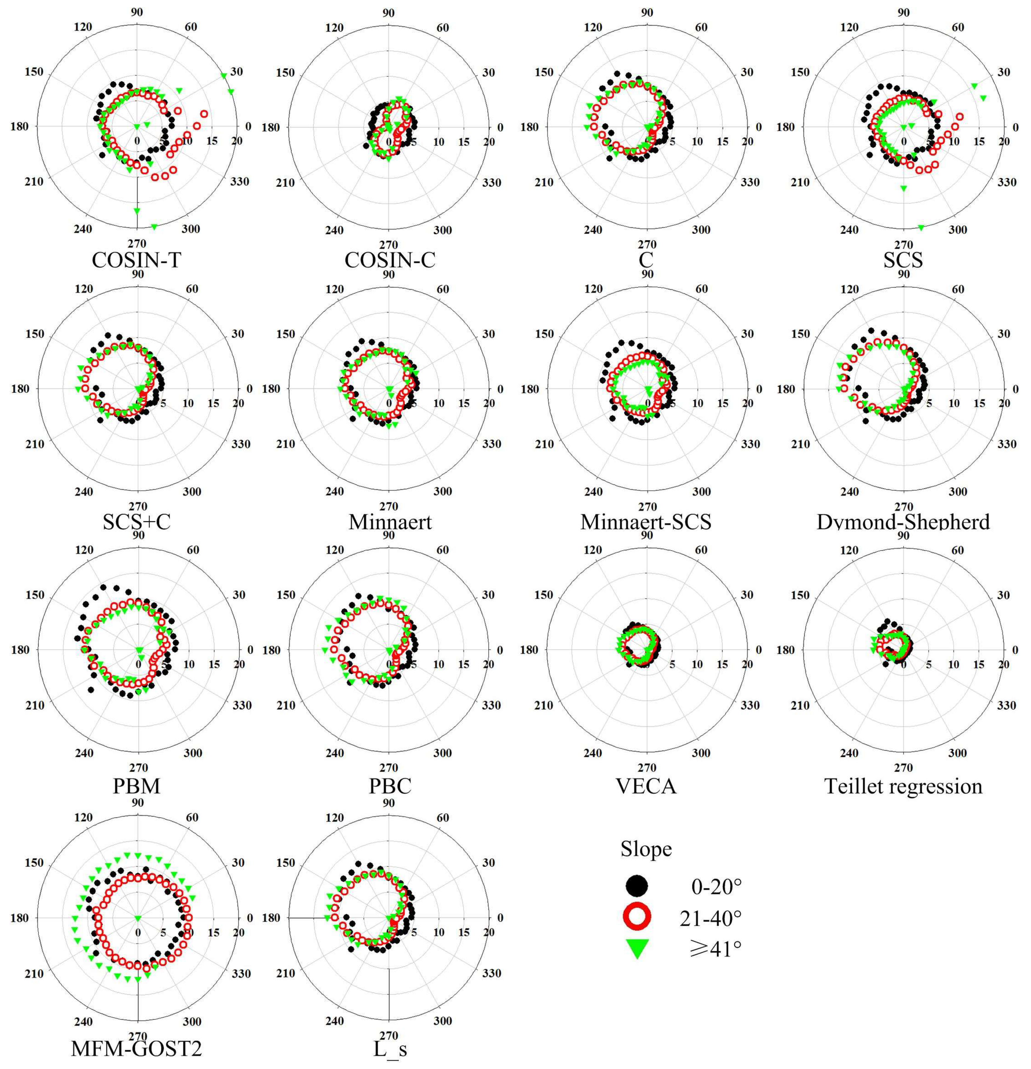
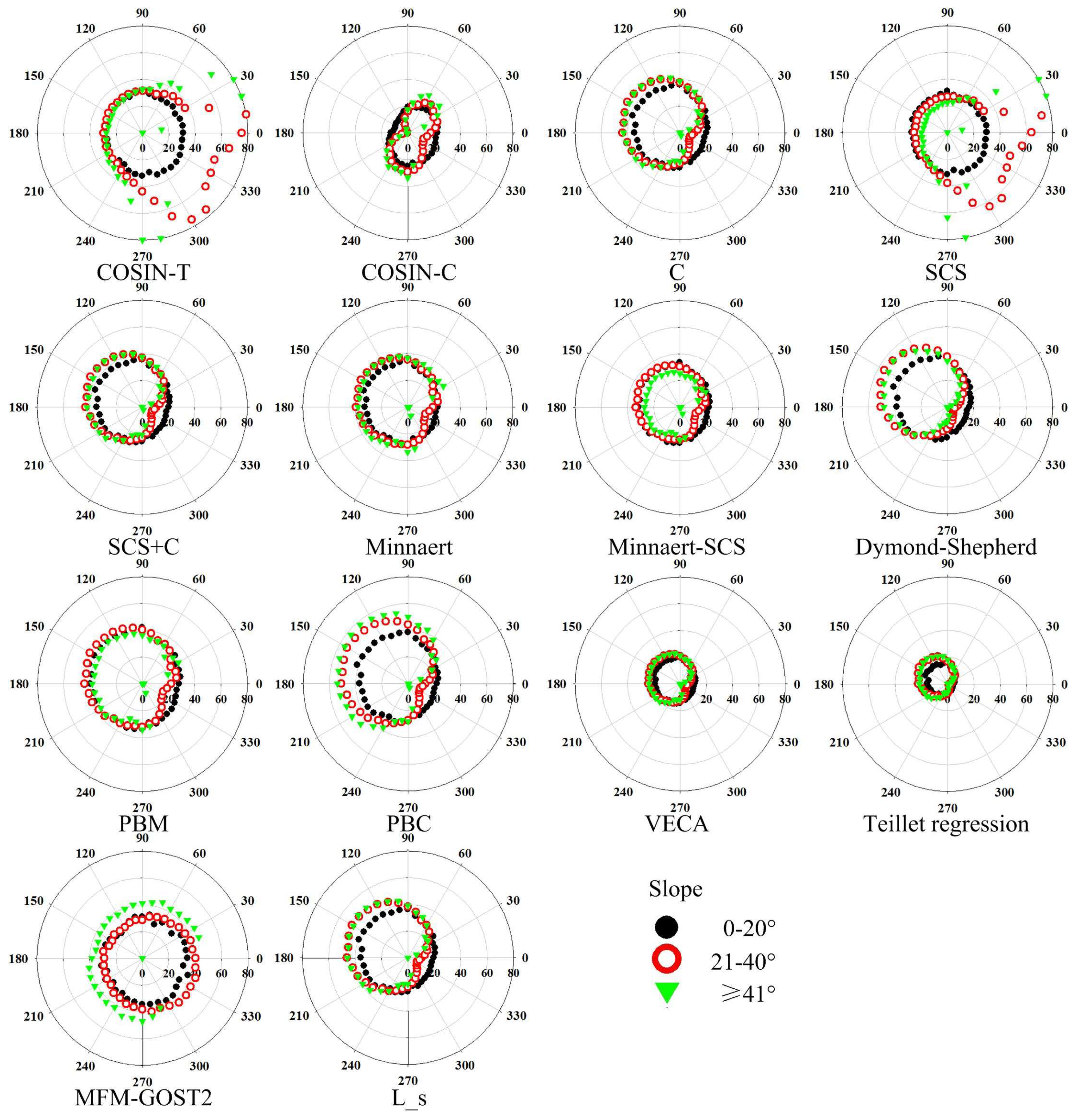
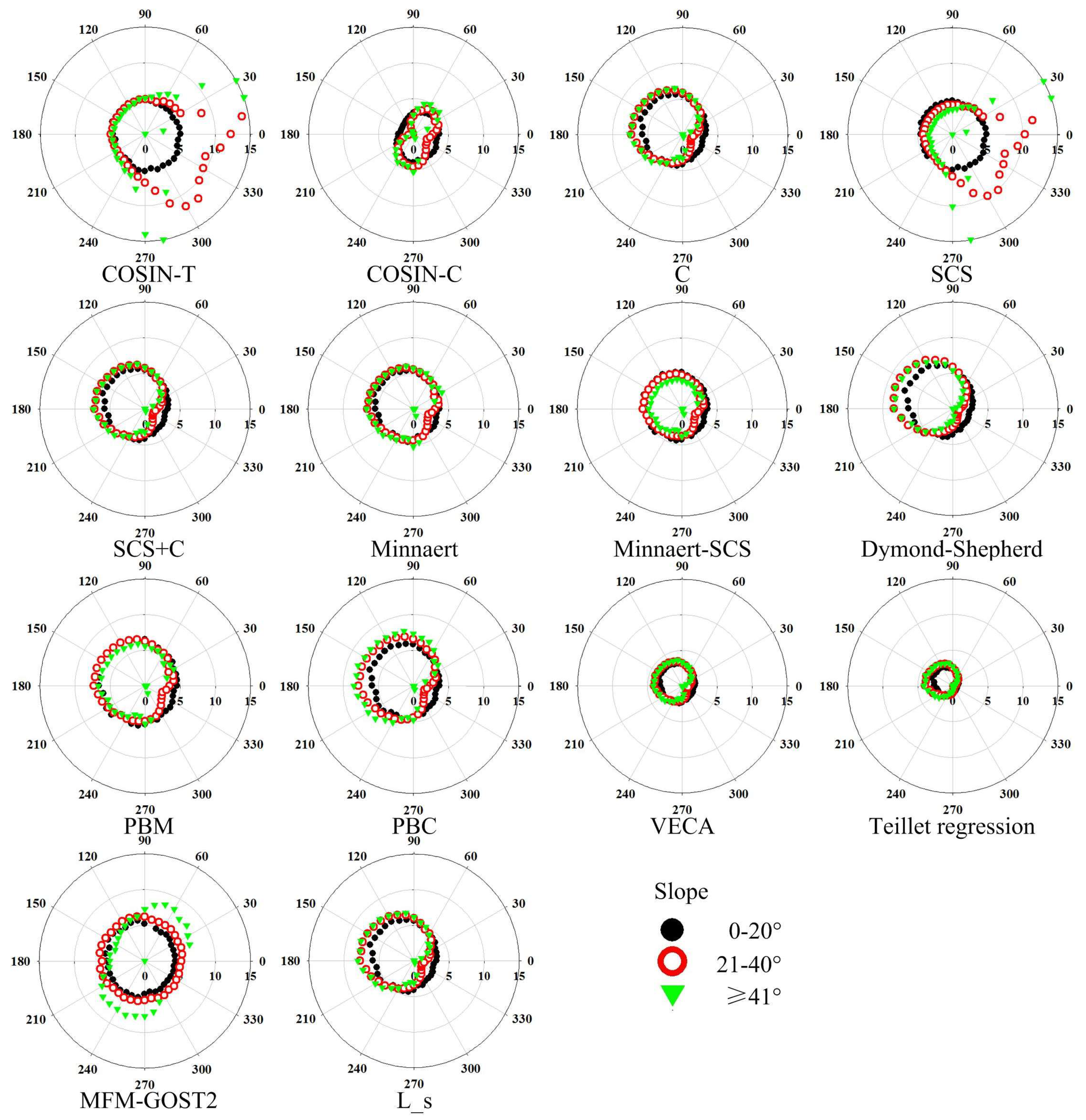
4.3. Statistical Analysis—The Rose Diagram

Figure 5, Figure 6 and Figure 7 show the rose diagrams of the radiances before and after topographic corrections. In the rose diagrams of uncorrected images (L_s), obvious topographic effects appear in the red, NIR, and SWIR bands, respectively. It can be found that the radiances decrease with the increasing angle between the solar azimuth angle and canopy aspect. In addition, radiances increase with slopes at sunny canopies and decrease with increasing slopes at shady canopies. For this reason, we found that the uncorrected radiances are nearly constants when canopy slopes are perpendicular to the direction of sunlight (aspects of sloping canopies are 67° and 247°, respectively) in this study. The constant values can be explained by the geometric optical theory of sloping canopies: the significant change of projected crown shadows makes the most striking divergences of canopy radiances when canopy slopes are along the sunlight direction (the azimuth angles between slope background and canopy are 0° and 180°, respectively), but projected crown shadows have minimal change (topographic independent) when canopy slopes are perpendicular to the sunlight direction (the azimuth angles between slope background and canopy are 90° and 270°, respectively). Therefore, the corrected radiances of the image should be close to the topographic independent values which are about 5–10 W/(m2·sr·μm), 30–40 W/(m2·sr·μm), and 4–6 W/(m2·sr·μm) in the red, NIR, and SWIR bands, respectively, in this study.
Most of the angular dependence of the uncorrected radiances is removed by the MFM-GOST2 method. The corrected radiances by MFM-GOST2 are close to the topographic independent values in all three bands. The positive comment is identical to that of the visual analysis and the linear relationship analysis. A few radiances of shaded slopes are vacant because the GOST2 model cannot be used for modeling the canopy radiances without direct sunlight contribution. The radiances at shaded slopes are overcorrected by both the COSIN_T and SCS corrections. The overestimations are enhanced as the canopy slopes increase. The result agrees well with those of the visual analysis. This indicates that the two methods may be applicable for canopies growing on gentle slopes. However, the positive results given by the linear relationship analysis of the two methods illustrate that the successful decorrelation does not mean that the corrected results are as expected. The corrected radiances by the VECA and Teillet regression corrections are greatly underestimated in the three bands. This also supports the negative results given by the visual analysis. However, the result of the linear relationship analysis shows marginal positive improvements. In addition, topography-induced high radiance values at sunlight slopes and low radiance values at shaded slopes are maintained after the VECA and Teillet regression corrections. The corrected radiances are underestimated after the COSIN_C correction. The visual analysis displays the same characteristics as the underestimation, but the linear relationship analysis shows successful decorrelation. The corrections by the C, PBC, and SCS + C methods are not evident in the rose diagram analysis. This coincides with both the visual and linear relationship analysis. The radiances corrected by the Minnaert and Minnaert-SCS corrections are close to the topographic-independent values for sunlit canopies but have a small improvement for shaded canopies. The results can also be found in the visual analysis but cannot be noticed by the linear relationship analysis. The radiances corrected by PBM show minor improvement compared with that of the uncorrected radiances. This is also captured by the visual analysis, but the linear relationship analysis gives a positive outcome. The Dymond-Shepherd correction enhances the topographic effects in this study. Both the visual analysis and the linear relationship analysis can support the enhancement of topographic effects.

5. Discussion

5.1. The MFM-GOST2 Correction

As expected, the MFM-GOST2 correction removes most of the topographic effects and achieves good performance in the visual analysis, linear relationship analysis, and rose diagram analysis. It is important to note, however, that there are also several issues that warrant attention. One important issue associated with the quality of corrected radiances is that the pre-built LUT should be big enough to cover canopy parameter combinations as much as possible for matching real canopy parameters over slopes. However, a big LUT may lead to increasing noise information for determining the final corrected radiance. On the other hand, MFM-GOST2 is a frame platform based on the LUT constructed by the GOST2 model. Various canopy parameters given by investigators may provide different LUTs, which finally produce different topographic correction results. Therefore, providing prior knowledge as much as possible will improve the accuracy of the topographic corrections. For example, an approximate range of canopy parameters given according to a landcover map helps to reduce unexpected information in the LUT construction process. In other words, the ranges of some canopy parameters listed in Table 2 can be specified and narrowed for constructing the LUT according to the prior knowledge for the benefit of the MFM inversion accuracy. In this way, the capacity of a LUT can also be optimized, although it is still unclear how to determine its best capacity. As for determining the final corrected radiances from the potential radiances after the LUT searching process, Soenen et al. [3] suggested using a median value. In this study, we calculated both the median and mean values of the potential radiances and found that there is almost no difference between the two corrections. Therefore, only the results using the mean value are shown in this study. Soenen et al. [3] indicate that one of the core advantages of a canopy reflectance model-based topographic correction method is the ability to explicitly account for a full variety of the main environmental, geometrical, structural, illumination, edaphic, and ecological factors that influence airborne and satellite image spectral response [39,40]. The experimental data of this case study is limited to specific forest canopies, solar, and view zenith angles. Actually, the MFM-GOST2 correction is theoretically suitable for any forest types, solar, and view zenith angles that are included in the simulations of GOST2. For this reason, MFM-GOST2 is superior to most other correction methods, such as its potential applications in topographic correcting multi-angular remotely sensed data (e.g., the CHRIS/PROBA data).
Another important issue is concerned with the following question: what spatial resolution is the MFM-GOST2 correction suitable for? Essentially, the MFM-based correction framework is spatial-resolution-independent. However, the spatial resolution is limited by the requirement of the forward canopy reflectance model, such as the GOST2 model. The basic principle of the GOST2 model is the geometric optical theory for canopies. As for the GOST2 model, the area of a canopy (a pixel) should be large enough to have sufficient tree crowns to fulfill the statistic requirement of the preset tree distribution, such as the Poisson distribution. However, an overly large area of a pixel may result in topographic variance which is different from the assumption of the invariant topography within a canopy of the GOST2 model. On the other hand, high spatial resolution remotely sensed data, such as the SPOT-7 satellite image data at 6 m spatial resolution, can be down-sampled to meet the statistic requirement of the GOST2 model. The 30 m × 30 m spatial resolution pixels of Landsat 8 images are suitable for the topographic condition of the study area. The corrected result by MFM-GOST2 supports this. Using the MFM-GOST2 method, the spatial resolution of remotely sensed images should be carefully determined depending on the intensity of topographic variation for a specific study area.
The third concern relates to the numeric efficiency of the MFM-GOST2 correction. Although the execution efficiency of GOST2 was greatly improved compared with that of the GOST model [26], the LUT construction process requires a lot of time because of the forward modeling of GOST2. For example, it takes about one month to develop such a big LUT for this study. However, the LUT is reusable for other studies. Therefore, the computational restriction can be relaxed after the initial LUT was developed. On the other hand, in order to speed up the MFM inversion procedure, the LUT was separated as thousands of sub-LUTs according to the given sun-canopy-sensor geometry in Table 2. Then records of the LUT can be loaded from the computer’s memory faster than before. However, the MFM inversion procedure is still not as fast as the twelve topographic correction methods in this study. Actually, the numeric efficiency of MFM-GOST2 depends on both the MFM inversion strategy and computer performance. For a higher numeric efficiency, it is worth exploring the better MFM inversion strategies in further studies.

5.2. The Evaluation Methods

The visual analysis is one of the most commonly used and immediate methods for evaluating topographic corrections. It depends entirely on the subjective experience of humans, and the final conclusion of a topographic corrected result is difficult to derive from the method. Previous studies have generally concluded that the success criterion in topographic correction is the decorrelation of the cosine of incidence angles and corrected radiances. However, we found that the decorrelation is not a sufficient condition to determine a successful topographic correction. This study shows that the decorrelation can be achieved by several topographic corrections, but topographic relief is still evident after these corrections, such as COSIN-C, COSIN-T, and SCS. Therefore, the linear relationship analysis cannot be used independently for evaluating the radiances after topographic corrections. In this study, the rose diagram analysis checks the variation of corrected radiances with slopes and aspects directly. It is superior in its detailed comparison of the radiances before and after correction under various surface topography conditions, and provides a quantitative evaluation supporting the visual analysis.

6. Conclusions

The MFM-GOST2 correction was developed based on the second version of the canopy reflectance model for sloping terrains-GOST2. The MFM-GOST2 correction and twelve generally used topographic correction methods were evaluated and compared via a case study by the visual analysis, the linear relationship analysis and the rose diagram analysis. This illustrates that the MFM-GOST2 correction shows good potential to remove the topographic effects of the remotely sensed radiances of sloping canopies. In addition, the rose diagram analysis provides positive support for the visual analysis. However, decorrelation of the linear relationship analysis is not a sufficient condition to prove the success of topographic corrections in this study because most of the unsuccessful corrections were not identified by the linear relationship analysis.
In this study, the bamboo forest with a relatively simple canopy structure was used as an example to compare the topographic correction methods. Although the MFM-GOST2 correction is superior in its clear physical background to consider canopy parameters without prior knowledge of canopies, and shows good performance in this study area, there is also a need to evaluate the correction method under more complicated cases in future studies. In addition, how to determine the proper capacity of LUT should also be a focus of further works.

Author Contributions

W.F., J.L., H.D., G.Z., and X.X. conceived and designed the experiments; W.F., Q.Z., G.Y., A.L., Y.Z., and B.X. performed the experiments and analyzed the data; J.L., Q.L.; and G.Z. provided with the guidance and gave important suggestions in the revisions; W.F. wrote the paper.

Acknowledgments

This work was supported in part by the National Science Foundation of China under Grant 41631180/D0106, by Zhejiang Provincial Natural Science Foundation of China under Grant No. LY18D010003, by the National Science Foundation of China under Grant 41601403/D0106 and Grant 41401418/D0106, and by the Talent Innovation Foundation of Zhejiang A&F University under Grant 2034020072.

Conflicts of Interest

The authors declare no conflict of interest.

References

  1. Kane, V.R.; Gillespie, A.R.; McGaughey, R.; Lutz, J.A.; Ceder, K.; Franklin, J.F. Interpretation and topographic compensation of conifer canopy self-shadowing. Remote Sens. Environ. 2008, 112, 3820–3832. [Google Scholar] [CrossRef]
  2. Szantoi, Z.; Simonetti, D. Fast and robust topographic correction method for medium resolution satellite imagery using a stratified approach. IEEE J. Sel. Top. Appl. Earth Obs. Remote Sens. 2013, 6, 1921–1932. [Google Scholar] [CrossRef]
  3. Soenen, S.A.; Peddle, D.R.; Coburn, C.A.; Hall, R.J.; Hall, F.G. Improved topographic correction of forest image data using a 3-D canopy reflectance model in multiple forward mode. Int. J. Remote Sens. 2008, 29, 1007–1027. [Google Scholar] [CrossRef]
  4. Li, X.W.; Strahler, A.H. Geometric-optical bidirectional reflectance modeling of the discrete crown vegetation canopy: Effect of crown shape and mutual shadowing. IEEE Trans. Geosci. Remote Sens. 1992, 30, 272–296. [Google Scholar] [CrossRef]
  5. Chen, J.M.; Leblanc, S.G. A 4-scale bidirectional reflection model based on canopy architecture. IEEE Trans. Geosci. Remote Sens. 1997, 35, 1316–1337. [Google Scholar] [CrossRef]
  6. Vanonckelen, S.; Lhermitte, S.; Ronpaey, A.V. The effect of atmospheric and topographic correction methods on land cover classification accuracy. Int. J. Appl. Earth Obs. 2013, 24, 9–21. [Google Scholar] [CrossRef]
  7. Chander, G.; Markham, B.L.; Helder, D.L. Summary of current radiometric calibration coefficients for Landsat MSS, TM, ETM+, and EO-1 ALI sensors. Remote Sens. Environ. 2009, 113, 893–903. [Google Scholar] [CrossRef]
  8. Hantson, S.; Chuvieco, E. Evaluation of different topographic correction methods for Landsat imagery. Int. J. Appl. Earth Obs. 2011, 13, 691–700. [Google Scholar] [CrossRef]
  9. Teillet, P.M.; Guindon, B.; Goodenough, D.G. On the slope-aspect correction of multispectral scanner data. Can. J. Remote Sens. 1982, 8, 84–106. [Google Scholar] [CrossRef]
  10. Civco, D.L. Topographic normalisation of Landsat Thematic Mapper digital imagery. Photogramm. Eng. Remote Sens. 1989, 55, 1303–1309. [Google Scholar]
  11. Gu, D.; Gillespie, A. Topographic normalization of Landsat TM images of forest based on subpixel Sun-Canopy-Sensor geometry. Remote Sens. Environ. 1998, 64, 166–175. [Google Scholar] [CrossRef]
  12. Soenen, S.A.; Peddle, D.R.; Coburn, C.A. SCS + C: A modified Sun-Canopy-Sensor topographic correction in forested terrain. IEEE Trans. Geosci. Remote Sens. 2005, 43, 2148–2159. [Google Scholar] [CrossRef]
  13. Smith, J.A.; Lin, T.L.; Ranson, K.L. The Lambertian assumption and Landsat data. Photogramm. Eng. Remote Sens. 1980, 46, 1183–1189. [Google Scholar]
  14. Reeder, D.H. Topographic Correction of Satellite Images Theory and Application. Ph.D. Thesis, Dartmouth College, Hanover, NH, USA, 2002. [Google Scholar]
  15. Dymond, J.R.; Shepherd, J.D. Correction of the topographic effect in remote sensing. IEEE Trans. Geosci. Remote Sens. 1999, 37, 2618–2619. [Google Scholar] [CrossRef]
  16. Lu, D.; Ge, H.; He, S.; Xu, A.; Zhou, G.; Du, H. Pixel-based Minnaert correction method for reducing topographic effects on the Landsat 7 ETM+ image. Photogramm. Eng. Remote Sens. 2008, 74, 1343–1350. [Google Scholar]
  17. Kobayashi, S.; Sanga-Ngoie, K. The integrated radiometric correction of optical remote sensing imageries. Int. J. Remote Sens. 2008, 29, 5957–5985. [Google Scholar] [CrossRef]
  18. Gao, Y.N.; Zhang, W.C. Variable Empirical Coefficient Algorithm for Removal of Topographic Effects on Remotely Sensed Data from Rugged Terrain. In Proceedings of the IEEE International Geosciences and Remote Sensing Symposium (IGARSS2007), Barcelona, Spain, 23–28 July 2007. [Google Scholar]
  19. Pimple, U.; Sitthi, A.; Simonetti, D.; Pungkul, S.; Leadprathom, K.; Chidthaisong, A. Topographic correction of Landsat TM-5 and Landsat OLI-8 imagery to improve the performance of forest classification in the mountainous terrain of Northeast Thailand. Sustainability 2017, 9, 258. [Google Scholar] [CrossRef]
  20. Riaño, D.; Chuvieco, E.; Salas, J.; Aguado, I. Assessment of different topographic corrections in Landsat-TM data for mapping vegetation types. IEEE Trans. Geosci. Remote Sens. 2003, 41, 1056–1061. [Google Scholar] [CrossRef]
  21. Meyer, P.; Itten, K.I.; Kellenberger, T.; Sandmeier, S.; Sandmeier, R. Radiometric corrections of topographically induced effects on Landsat TM data in an alpine environment. ISPRS J. Photogramm. Remote Sens. 1993, 48, 17–28. [Google Scholar] [CrossRef]
  22. Peddle, D.R.; Teillet, P.M.; Wulder, M.A. Chapter 7—Radiometric image processing. In Remote Sensing of Forest Environments: Concepts and Case Studies; Wulder, M.A., Franklin, S.E., Eds.; Springer: New York, NY, USA, 2003; pp. 181–208. ISBN 978-1-4615-0306-4. [Google Scholar]
  23. Gao, Y.N.; Zhang, W.C. A simple empirical topographic correction method for ETM+ imagery. Int. J. Remote Sens. 2009, 20, 2259–2275. [Google Scholar] [CrossRef]
  24. Karathanassi, V.; Andronis, V.; Rokos, D. Evaluation of the topographic normalization methods for a Mediterranean forest area. Int. Arch. Photogramm. Remote Sens. 2000, 33, 654–661. [Google Scholar]
  25. Schaaf, C.B.; Li, X.W.; Strahler, A.H. Topographic effects on bidirectional and hemispherical reflectances calculated with a geometricoptical canopy model. IEEE Trans. Geosci. Remote Sens. 1994, 32, 1186–1193. [Google Scholar] [CrossRef]
  26. Fan, W.L.; Li, J.; Liu, Q.H. GOST2: The improvement of the canopy reflectance model GOST in separating the sunlit and shaded leaves. IEEE J. Sel. Top. Appl. Earth Obs. Remote Sens. 2015, 8, 1423–1431. [Google Scholar] [CrossRef]
  27. Fan, W.L.; Chen, J.M.; Ju, W.M.; Zhu, G.L. GOST: A geometric–optical model for sloping terrains. IEEE Trans. Geosci. Remote Sens. 2014, 52, 5469–5482. [Google Scholar]
  28. Fan, W.L.; Chen, J.M.; Ju, W.M.; Nesbitt, N. Hybrid geometric optical-radiative transfer model suitable for forests on slopes. IEEE Trans. Geosci. Remote Sens. 2014, 52, 5579–5586. [Google Scholar]
  29. Peddle, D.R.; Johnson, R.L.; Cihlar, J.; Leblanc, S.G.; Chen, J.M.; Hall, F.G. Physically-based inversion modeling for unsupervised cluster labeling, independent forest classification and LAI estimation using MFM-5-Scale. Can. J. Remote Sens. 2007, 33, 214–225. [Google Scholar] [CrossRef]
  30. Vicente-Serrano, S.M.; Pérez-Cabello, F.; Lasanta, T. Assessment of radiometric correction techniques in analyzing vegetation variability and change using time series of Landsat images. Remote Sens. Environ. 2008, 112, 3916–3934. [Google Scholar] [CrossRef]
  31. Li, F.Q.; David, L.B.; Jupp, M.T.; Leo, L.; Norman, M.; Lewis, A.; Held, A. A physics-based atmospheric and BRDF correction for Landsat data over mountainous terrain. Remote Sens. Environ. 2012, 124, 756–770. [Google Scholar] [CrossRef]
  32. Tan, B.; Masek, J.G.; Wolfe, R.; Gao, F.; Huang, C.Q.; Vermote, E.F.; Sexton, J.O.; Ederer, G. Improved forest change detection with terrain illumination corrected Landsat images. Remote Sens. Environ. 2013, 136, 469–483. [Google Scholar] [CrossRef]
  33. Song, C.; Woodcock, C.E.; Seto, K.C.; Lenney, M.P.; Macomber, S.A. Classification and change detection using Landsat TM data: When and how to correct atmospheric effects? Remote Sens. Environ. 2001, 75, 230–244. [Google Scholar] [CrossRef]
  34. Wu, Q.; Jin, Y.; Fan, H. Evaluating and comparing performances of topographic correction methods based on multi-source DEMs and Landsat-8 OLI Data. Int. J. Remote Sens. 2016, 37, 4712–4730. [Google Scholar] [CrossRef]
  35. Richter, R.; Kellenberger, T.; Kaufman, H. Comparison of topographic correction methods. Remote Sens. 2009, 1, 184–196. [Google Scholar] [CrossRef] [Green Version]
  36. Ghasemi, N.; Mohammadzadeh, A.; Sahebi, M.R. Assessment of different topographic correction methods in ALOS AVNIR-2 data over a forest area. Int. J. Digit. Earth 2013, 6, 504–520. [Google Scholar] [CrossRef]
  37. Reese, H.; Olsson, H. C-correction of optical satellite data over alpine vegetation areas: A comparison of sampling strategies for determining the empirical C-parameter. Remote Sens. Environ. 2011, 115, 1387–1400. [Google Scholar] [CrossRef]
  38. Zhang, Y.; Li, X.; Wen, J.; Liu, Q.; Yan, G. Improved topographic normalization for Landsat TM images by introducing the MODIS surface BRDF. Remote Sens. 2015, 7, 6558–6575. [Google Scholar] [CrossRef]
  39. Hall, F.G.; Knapp, D.E.; Huemmrich, K.F. Physically based classification and satellite mapping of biophysical characteristics in the southern boreal forest. J. Geophys. Res. Atmos. 1997, 102, 29567–29580. [Google Scholar] [CrossRef]
  40. Peddle, D.R.; Hall, F.G.; Ledrew, E.F. Spectral mixture analysis and geometric-optical reflectance modeling of boreal forest biophysical structure. Remote Sens. Environ. 1999, 67, 288–297. [Google Scholar] [CrossRef]
Figure 1. The flowchart of the MFM-GOST2 method.
Remotesensing 10 00717 g001
Figure 2. Location of the study area in the north of Anji County, Zhejiang, China.
Remotesensing 10 00717 g002
Figure 3. The topographic factors derived from the digital elevation model (DEM). The black areas in “Shadows” represent that the canopies do not receive the direct solar radiation.
Remotesensing 10 00717 g003
Figure 4. The original and corrected images by MFM-GOST2 and the twelve topographic correction methods. (a) is in the red band (Landsat-8 OLI band 4); (b) is in the NIR band (Landsat-8 OLI band 5); (c) is in the SWIR band (Landsat-8 OLI band 6); and (d) is the false color composites of Landsat-8 OLI (band 6-5-4). Radiances of the false color composites images were multiplied by 2.5 for improving the visually inspection. L_s is the uncorrected image.
Remotesensing 10 00717 g004aRemotesensing 10 00717 g004b
Figure 5. Changes of mean radiances in the red band with the aspect at fixed slope intervals in the study area. The polar angle represents the aspect of background (°), and the radius represents the value of radiances (W/(m2·sr·μm)). L_s is the uncorrected radiance.
Remotesensing 10 00717 g005
Figure 6. Changes of mean radiances in the NIR band with the aspect at fixed slope intervals in the study area. The polar angle represents the aspect of background (°), and the radius represents the value of radiances (W/(m2·sr·μm)). L_s is the uncorrected radiance.
Remotesensing 10 00717 g006
Figure 7. Changes of mean radiances in the SWIR band with the aspect at fixed slope intervals in the study area. The polar angle represents the aspect of background (°), and the radius represents the value of radiances (W/(m2·sr·μm)). L_s is the uncorrected radiance.
Remotesensing 10 00717 g007
Table 1. Overview of the twelve topographic correction algorithms.
ModelEquationsReferences
COSIN-T L c = L cos ( θ s ) cos ( i ) [9]
COSIN-C L c = L [ 1 + cos ( i ) ¯ cos ( i ) cos ( i ) ¯ ] [10]
C-correction L c = L cos ( θ s ) + c cos ( i ) + c [9]
SCS L c = L cos ( θ s ) cos ( θ g ) cos ( i ) [11]
SCS + C L c = L cos ( θ s ) cos ( θ g ) + c cos ( i ) + c [12]
Minnaert L c = L [ cos ( θ s ) cos ( i ) ] k [13]
Minnaert-SCS L c = L cos k ( θ s ) cos ( θ g ) cos k ( i ) [14]
Dymond-Shepherd L c = L cos ( i ) + cos ( e ) cos ( θ v ) + cos ( θ s ) [15]
PBM L c = L cos ( θ g ) [ cos ( θ g ) cos ( i ) ] k [16]
PBC L c = L cos ( θ s ) + C λ h 0 1 cos ( i ) + C λ h 0 1 h [17]
VECA L c = L L ¯ a cos ( i ) + b [18]
Teillet regression L c = L a cos ( i ) b + L ¯ [9]
Note: L C and L are the corrected and uncorrected radiance (W/(m2·sr·μm)), respectively. θ s is the solar zenith angle and θ g is the slope of terrains. c is the quotient between the slope a and intercept b of the regression L = a cos ( i ) + b . L ¯ is the mean value of L . i and e are the incident and exitance angles of sunlight over slopes, respectively. cos ( i ) = cos ( θ s ) cos ( θ g ) + sin ( θ s ) sin ( θ g ) cos ( ϕ s ϕ g ) , where ϕ s and ϕ g are the azimuth angles of sunlight and slopes, respectively. cos ( e ) = cos ( θ v ) cos ( θ g ) + sin ( θ v ) sin ( θ g ) cos ( ϕ v ϕ g ) , where θ v and ϕ v are the view zenith and azimuth angles, respectively. cos ( i ) ¯ is the mean value of cos ( i ) . k is the Minnaert constant which takes values between 0 and 1, and it can be calculated as the slope of the regression between x = log ( cos ( θ g ) cos ( i ) ) and y = log ( L cos ( θ g ) ) . C λ is the quotient of intercept and slope of the regression line between x and y . h 0 = ( π + 2 θ s ) / ( 2 π ) and h = ( 1 θ g ) / π .
Table 2. The preset canopy parameters for constructing the look up table (LUT) using the GOST2 model.
Canopy ParametersValues
Stem density (stem/ha)1300, 4000, 6000, 10,000
Tree distributionneyman, poisson
Radius of trees (m)0.5, 1.5, 2.5, 3.5
Under-branch height (m)1, 7, 15
Crown height (m)0.5, 5.5, 10.5, 15.5
Leaf angular distribution (G)0.5
Clumping index (ΩE)0.6, 0.8, 1
Leaf area index of a crown (m2/m2)1, 2, 4, 6, 8, 10, 12
Leaf shapecircular, spherical
Crown shapecone, cone + cylinder, ellipsoid
Solar zenith/azimuth angle (°)97 angular combinations
View zenith/azimuth angle (°)75 angular combinations
Slope (°)0, 10, 20, 30, 40, 50
Aspect (°)from 0 to 360 at intervals of 20
Leaf BRF (the red band)0.02, 0.07, 0.1
Leaf transmittance (the red band)0.012, 0.05, 0.06
Background BRF (the red band)0.1, 0.16, 0.45
Leaf BRF (the NIR band)0.2, 0.35, 0.4, 0.5, 0.7
Leaf transmittance (the NIR band)0.15, 0.2, 0.3, 0.5
Background BRF (the NIR band)0.15, 0.23, 0.25, 0.3
Leaf BRF(the SWIR band)0.1, 0.3, 0.5
Leaf transmittance (the SWIR band)0.1, 0.25, 0.45
Background BRF (the SWIR band)0.2, 0.4, 0.6
BRF, bidirectional reflectance factor; NIR, near infrared; SWIR, short-wave infrared.
Table 3. R2 between the cosine of the incident angle and the corrected/uncorrected radiances in the red, NIR and SWIR bands, respectively.
MethodsRedNIRSWIR
Uncorrected0.37140.47560.5179
MFM-GOST20.00040.03370.0004
COSIN_T0.02020.07640.0855
COSIN_C0.07780.23400.2566
C-correction0.35850.41790.4605
SCS0.02070.08250.0912
SCS + C0.35730.41590.4583
Minnaert0.08560.10710.1320
Minnaert-SCS0.07430.09470.1160
Dymond–Shepherd0.47650.64320.6774
PBM0.07970.10000.1224
PBC0.27560.40350.3564
VECA0.35840.41790.4605
Teillet regression0.33360.37200.4134

