Characterizing Land Surface Anisotropic Reflectance over Rugged Terrain: A Review of Concepts and Recent Developments

Abstract

Rugged terrain, including mountains, hills, and some high lands are typical land surfaces around the world. As a physical parameter for characterizing the anisotropic reflectance of the land surface, the importance of the bidirectional reflectance distribution function (BRDF) has been gradually recognized in the remote sensing community, and great efforts have been dedicated to build BRDF models over various terrain types. However, on rugged terrain, the topography intensely affects the shape and magnitude of the BRDF and creates challenges in modeling the BRDF. In this paper, after a brief introduction of the theoretical background of the BRDF over rugged terrain, the status of estimating land surface BRDF properties over rugged terrain is comprehensively reviewed from a historical perspective and summarized in two categories: BRDFs describing solo slopes and those describing composite slopes. The discussion focuses on land surface reflectance retrieval over mountainous areas, the difference in solo slope and composite slope BRDF models, and suggested future research to improve the accuracy of BRDFs derived with remote sensing satellites.

1. Introduction

Rugged terrain covers approximately 24% of the Earth’s land surface, plays an important role in the complex earth system, and forms a unique mountainous climate and ecosystem. Accurately estimating land surface variables over mountainous areas is of great importance for global hydrological and meteorological forecasts, as well as global ecological and environmental monitoring. Taking the benefits of advanced satellite instrumentation and accurate remote sensing modeling, topographic effects can be considered and neutralized in applications of surface parameter retrievals, such as improved land cover and land type mapping [1,2], key parameters of mountain radiation, and energy budget (albedo, land surface temperature (LST), and solar radiation) [3,4,5] and vegetation structure parameters (normalized difference vegetation index(NDVI), leaf area index (LAI), and fractional photosynthetically active radiation (FPAR)) [6,7]. Therefore, remote sensing satellite technique development over rugged terrain is crucial for extending remote sensing applications from flat surfaces to mountainous areas.

Remote sensing of anisotropic reflectance relates the land surface scattering behavior to its optics and structure, which is described with the bidirectional reflectance distribution function (BRDF) [8] and can be observed in optical remote sensing. To retrieve BRDF properties of the land surface is the basis for land surface’s physical parameter inversions [9,10,11,12], due to its structural information observed from different angles. In contrast, angular effects on surface reflectance should be removed by BRDF correction to normalize the reflectance [13,14,15] to implement classification and dynamic monitoring [16]. Thus, modeling the land surface BRDF and developing a corresponding remote sensing product is important for scientific research and remote sensing applications. However, rugged terrain complicates BRDF modeling by changing the amount of radiation detected by the sensor [17,18,19,20]. Generally, topography alters the illumination and viewing geometry and generates a relief shadow, observation masking, and multiple scattering, this results in the intense topographic dependence on total incident and reflectance radiance, which distorts BRDF characteristics [4,21]. The BRDF characteristics varies with wavelength and shows a BRDF wavelength dependence in surfaces of greater roughness [22,23]. Without considering the topographic effects on the land surface BRDF, the anisotropic reflectance estimation relative errors could be larger than 58% [24]. Therefore, the current remote sensing BRDF concept and modeling over rugged terrain should consider the topographic effects.

Previous studies have focused on the influence of geometric characteristics on the radiative transfer process over rugged terrain. Thus, the topographic correction models have first attempted to reduce topographic effects on reflectance [18,19,25,26]. Recently, there have been concerns about BRDF modeling over rugged terrain [17,20,21,27]. However, the operational BRDF product algorithm over rugged terrain is still being researched because it involves a complex process, which includes multi-angular reflectance dataset processing, an operational BRDF algorithm and its inversion method coupled with topography. From this perspective, high quality atmospheric correction that is used to obtain land surface reflectance is also the basic task to derive the rugged surface BRDF. Investigations have proven that the atmospheric correction of different resolution remote sensing data needs to consider the influence of topography [28,29]. However, with the decrease in spatial resolution, the influence of topography on pixel scale reflectance will gradually decrease. This causes a lot of the low resolution land surface reflectance to ignore the effects of topography during atmospheric correction (e.g., moderate resolution imaging spectroradiometer (MODIS) reflectance).The reflectance that does consider the topographic influence focuses on only the relatively high resolution remote sensing data (e.g., Landsat Thematic Mapper (Landsat/TM). Consequently, dominant BRDF modeling over rugged terrain occurs on an infinite slope surface [17,20,21,27]. However, the focus of low resolution remote sensing data is not the topography influence at the pixel level, but the topography influence at the sub-pixel level [29,30,31]. There should be a robust relationship between these two different anisotropic reflectance resolution. Thus, the characterization of land surface anisotropic reflectance over rugged terrain should be implemented from a systematic perspective by analyzing the critical scientific problems and reviewing current algorithms, which will benefit algorithm developers and broaden the interests of surface BRDF users.

In this paper, remote sensing BRDF modeling over rugged terrain according to the presented research chain is comprehensively reviewed, and the aim is to find an operational BRDF product potential solution for rugged terrain. This is important for quantitative remote sensing applications in mountainous areas. The paper is organized as follows: first, we analyzed the topographic effects on the BRDF and its scientific problems in Section 2. Second, the methods to solve the atmospheric correction and obtain the multi-angular reflectance are briefed in Section 3. The two kinds of BRDF modeling are described based on evolution histories in Section 4 and Section 5, according to the spatial resolution between the digital elevation model (DEM) and remote sensing pixel. Then, we analyzed the challenges and opportunities for BRDF product generation over rugged terrain in Section 6. Finally, we summarize this paper.

2. BRDF in Rugged Terrain

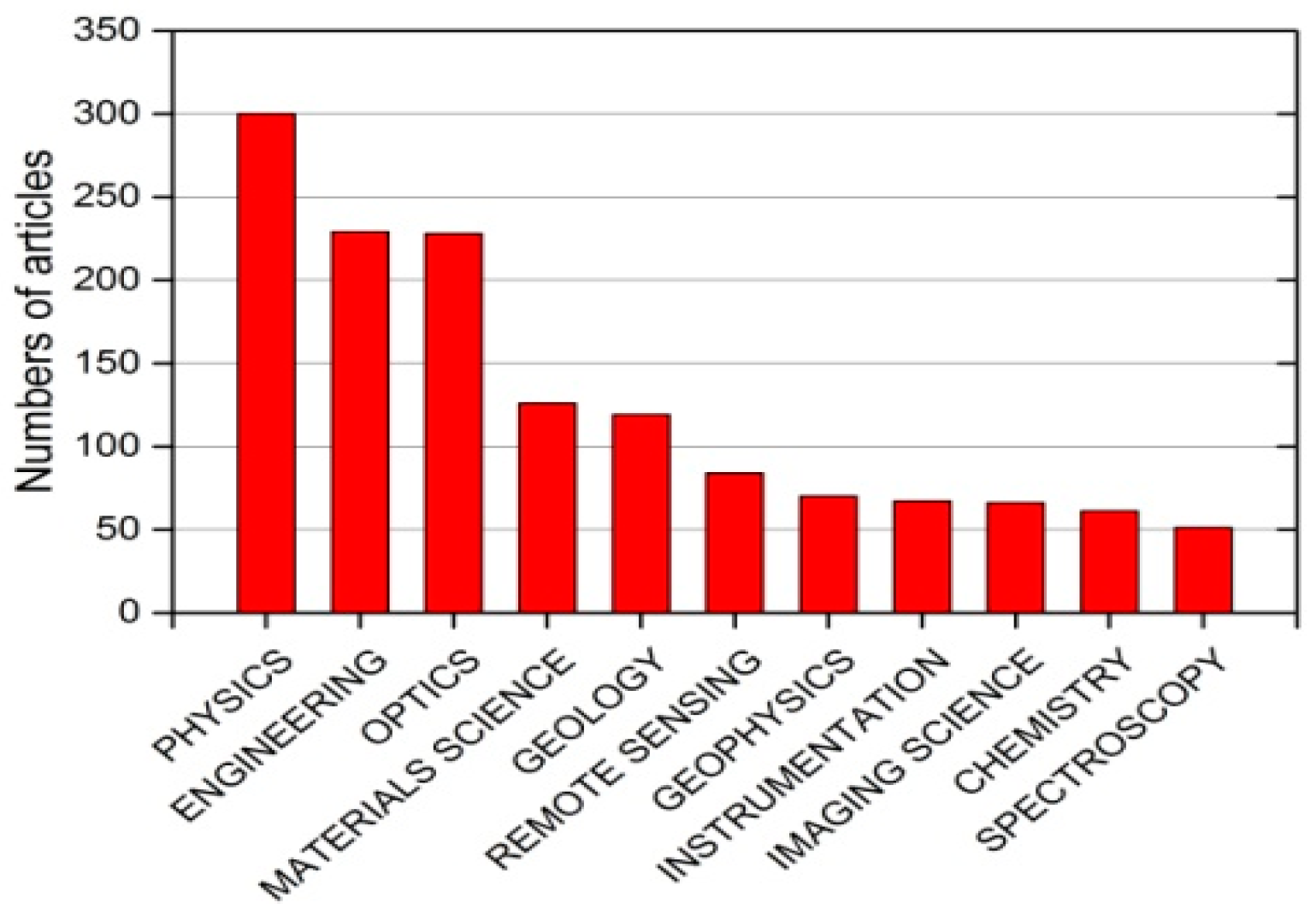
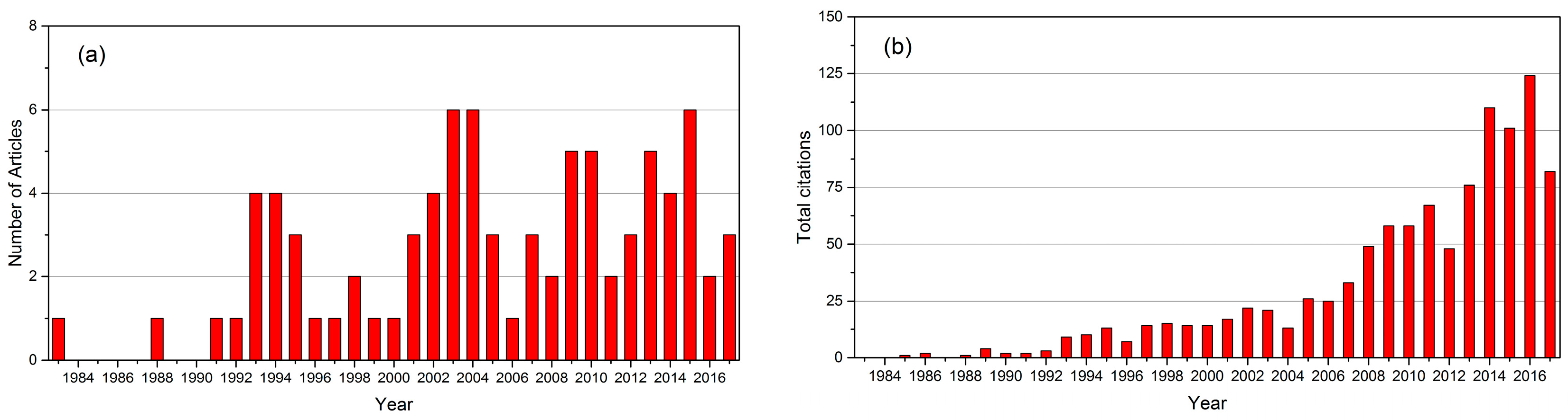
2.1. Literatures Review

A review of the current literature is one of the best ways to clearly understand the timeline and milestones in BRDF research over rugged terrain. In this paper, we searched for articles titles matching the relevant key words about BRDF and rugged terrain on the Web of Science website, Thomson Reuter. BRDF has seven relevant query words: “reflect*”, ”reflectance*”, “non*Lambertian”, “BRDF”, “BRF”, “bi-directional reflect*”, and “bidirectional reflect”, “multiangle”, “multi-angle”, “multiangular” and “multi-angular”. Rugged terrain has ten relevant query words: “mountain*”, “hill*”, “rugged terrain*”, “complex terrain*”, “topograph*”, “slope*”, “sloping terrain*”, “rough* surface*”, “random surface*”, and “roughness”. To exclude the irrelevant articles, we further screened the search results by subject and keywords. Finally, the articles about BRDF modeling over rugged terrain were collected from the Web of Science platform for citation statistics and analysis. Figure 1 shows the articles that were contributed by different research fields in recent decades. The results show that BRDF modeling over rugged terrain is of great importance in many scientific and engineering fields, including physics, engineering, optics, materials science, geology, remote sensing, geophysics, instrumentation, image science, chemistry, and spectroscopy. Judging by the number of articles, BRDF modeling over rugged terrain ranks sixth in remote sensing field.

Figure 2a,b shows the annual publications and citations from 1983 to 2017 in the field of remote sensing. Since 1993, there have been several articles published every year. The variation in the number of published papers on this subject have followed a periodical pattern. In some characteristic years, the number of published paper is as many as six. In comparison, the citations of these published papers grow smoothly by year, especially since 2006, which is when the numbers of citations showed a rapid increase. This demonstrates that the subject of BRDF modeling over rugged terrain has received increasing attention and has gradually become a hotspot in studies of quantitative remote sensing.

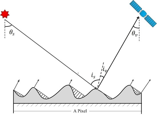
2.2. BRDF Definition and Its Topographic Effects

BRDF is defined mathematically as the ratio of the radiance $L_r$ which is reflected by the target surface into a specific direction, to the collimated solar incident irradiance $E_s$ on the same surface [32]. Two basic assumptions are implied in the current remote sensing BRDF quantity, which is shown in Equation (1) [33,34], and the assumptions are as follows: (1) the target surface is assumed to be a horizontal plane, and (2) the target surface is homogeneous with a uniform incident irradiance and outgoing irradiance. Namely, the radiative flux interaction and exchange is equivalent at every point over the target surface.

$$BRDF({\Omega }_s,{\Omega }_v)=\frac{d{L}_r({\Omega }_s,{\Omega }_v)}{d{E}_s({\Omega }_s)}$$

(1)

where ${\Omega }_s$ and ${\Omega }_v$ indicate the illumination and viewing geometry, respectively.

However, steep rugged terrain changes local illumination and viewing geometry because the normal of the slope surface is not consistent with the vertical direction (shown in Figure 3), which is results in heterogeneous incident irradiances due to the three-dimensional (3-D) structure configuration of vegetation and topography [34]. Specifically, the slopes facing toward the sun will receive more illuminated irradiance than the slopes that are away from the sun [18]. The diffuse irradiance reflected from adjacent slopes will increase the global incident irradiance of the slope surface, and the distribution of shadowing and observation masking have a notable effect on the pixel reflectance [29,35]. Therefore, the question of how to describe these topographic effects and the radiation redistribution is a core concern in the BRDF model over rugged terrain. It is concluded that to accurately model BRDF over rugged terrain, it should be coupled with the terrain information supplied by a DEM.

A spatial scale match between the DEM and remote sensing image pixel should be emphasized prior to coupling. According to the relationship between the spatial resolution of the available DEM and remote sensing pixel, the modeled topographies on the remote sensing pixel are classified into solo slope and composite slope (Figure 4). Under the assumption of the current DEM having a 30 m spatial resolution, the solo slope means that those remote sensing pixels have a spatial resolution comparable to the DEM dataset, and there is only a single slope surface, such as the Landsat/TM images, which have a 30 m spatial resolution. The composite slope refers to the situation when the remote sensing instrument with a large instantaneous field of view (IFOV) covers an area of few kilometers, which is result in a spatial resolution lower than the DEM dataset. There are numerous solo slopes contained within a remote sensing pixel. For example, the MODIS and advanced very high-resolution radiometer (AVHRR) sensors have a km-scale spatial resolution. However, if the remote sensing pixels have higher spatial resolution than the DEM, resampling the DEM to the same spatial resolution of the remote sensing image pixel is necessary. Otherwise, a higher resolution DEM should be provided.

The largest difference between topographic effects for these two types lies in the complex heterogeneous incident irradiance and topographic shadowing [4,29]. The pixel level topographic effect dominates the solo slope, including local geometry alteration, shadow cast, and diffuse irradiance reflected from adjacent slopes. In addition, with the lower spatial resolution, the topographic effects on BRDF become weaker due to a smooth overall slope [36]. However, in these cases, the sub-pixel level topographic effects are significant. Specifically, the sub-pixel level topographies affect the distributions of incident and reflected radiance by the distribution of sub-slope, sub-aspect, amount of shadow, and masking, which is leads to distorted BRDF characteristics.

Because the BRDF quantity is defined as the ratio of two infinitesimal surfaces, it is a theoretical concept and cannot be directly measured [13]. In remote sensing, the bidirectional reflectance factor (BRF) is adopted as a substitute for BRDF to describe the surface anisotropic scattering property [8,37]. BRF is defined as the ratio of reflected radiance from a target surface to that from an ideal and diffuse reference plane under identical illumination and viewing conditions. Thus, a key issue is how to define the reference plane when modeling the surface BRF. The horizontal reference plane at the highest point is widely favored in BRF models over a composite slope, which is shown in Figure 5 [29,30,35]. However, different opinions exist about a reference plane for the solo slope BRF model. Some physical-based analytical models adopt the reflectance of a slope-parallel white plane to calibrate surface BRF [17,21,27]. The derived reflectance is known as the slope BRF. The other analytical and most of 3-D computation BRF models are based on the horizontal reference plane, regardless of the underlying topography [20,38,39].

2.3. Model Building Procedures and Scientific Problems

Many efforts have been devoted to investigating the topographic effects on surface BRDF. The comprehensive and systematic investigation of sloped surface BRDF estimation is crucial to understanding the basic theory and the scientific problems that are involved with the BRDF over rugged terrain. According to the relationship between the DEM scale and remote sensing pixel spatial resolution, two cases of BRDF modeling over rugged terrain are presented in Figure 6: solo slope BRDF modeling and composite slope BRDF modeling. A self-consistent solution and a validation technique for these two BRDFs should be emphasized in this procedure.

Thus, to derive a desired BRDF product, which describes the BRDF properties of the slope surface, a suitable and robust BRDF model is the basis for retrieval of the anisotropic reflectance distribution with multi angle satellite reflectance data. The following three key issues are needed to be addressed when modeling surface BRDF over rugged terrain.

(1) How should the solo slope and composite slope anisotropic reflectance properties be described?

Solo slope and composite slope surfaces have different topographic effect mechanisms in the BRDF, which leads to different core sensitivity factors considered in remote sensing BRDF modeling. Accurately building a BRDF model depends on how the topographic characteristics are parameterized. The pixel-level topographic effect dominates the reflectance of the solo slope through the alteration of local incidence and viewing geometry, as well as the distribution of the illuminated irradiance [20,29]. However, this effect is relatively small for the composite slope BRDF, and the sub-pixel level topographic effects become the primary factors, which include the shadow, distribution of sub-topographic slope and aspect statistic, and the redistribution of radiation within a remote sensing pixel [4,31].

(2) How can we implement the solo slope or composite slope atmospheric correction to correctly derive reflectance?

Currently, the surface anisotropy reflectance, coupled with atmospheric parameters, is derived from the airborne and satellite remote sensing observations. The second simulation of the satellite signal in the solar spectrum radiative transfer process (6S) [40] model and the MODerate resolution atmospheric TRANs mission (MODTRAN) [41] model are the two methods to describe the atmospheric effects and can be used to retrieve the land surface reflectance from the top of the atmosphere radiance. The topographic effect is always neglected in these algorithms. Some efforts have been made to extend the 6S atmospheric correction algorithm, coupled with a topography consideration for a solo slope [18,19]. For a composite slope, the topographic effects on the atmospheric correction process are not included, because the slope of the pixel level is considered as flat. Otherwise, if the orientation of sub-topography is statistically dependent on the overall slope and aspect, the atmospheric correction should be coupled with topography.

(3) How can we develop the BRDF (BRF) validation technique and conduct experiments over rugged terrain?

When compared with flat surfaces, the spatial and temporal heterogeneity of surface BRDF appears more obvious over mountainous areas. The validation of the mountainous surface BRDF is an important issue, which includes sampling strategy and respective experiment conduction. With current observations covering several scales from ground measurements with ground-based instruments, meter-scale with unmanned aerial vehicles and km-scale with satellites, the multi-scale validation technique may potentially address this issue.

3. Remote Sensing Atmospheric Correction over Rugged Terrain

The BRDF properties of land surfaces are commonly retrieved against multiple directional reflectance to sufficiently sample anisotropy. Thus, it is necessary that the atmospheric correction is completed prior to the BRDF retrieval. However, the topography intensely affects the atmospheric correction, and consequently, also affects the land surface reflectance. Without DEM consideration in the atmospheric correction, the reflectance is varied in its response to similar topographic features, where the solar and sensor geometries correspond to a flat surface. According to Figure 5, the corrected reflectance without a DEM is not the reflectance referenced to the slope BRF defined a slope-parallel reference plane or the remote sensing BRF defined a horizontal reference plane, where the sensor view angle is the local angle corresponding to the slope surface. Although topographic correction can normalize the reflectance to that of flat surface, such as C correction [42], sun-canopy-sensor (SCS) correction [43], and their integrated method [44], the reflectance is still not applicable to the slope surface BRDF model retrieval due to its contradiction with the geometry defined slope of the BRDF model. To obtain an accurate reflectance over rugged terrain, the atmospheric correction should be coupled with topography, which is based on the mountain radiation transfer prototype model and DEM.

3.1. Lambertian-Based Atmospheric Correction

The mountain radiation transfer algorithms describe the radiance received by the sensor over a mountainous area. On rugged terrain, the irradiance at the target surface is composed of solar direct irradiance $E_s$, sky diffuse irradiance $E_d$, and adjacent terrain reflected irradiance $E_a$, which are shown in Figure 7.

Direct solar radiation over rugged terrain is the most important component of the total surface radiation that reaches to the surface. When compared with flat surfaces, this depends on the relative local incident angle between the sun and the normal to slope surface. Therefore, the direct solar radiation changes with different slope surfaces. The sky diffuse irradiance will be reduced when the sky dome overlying a surface is not an integrated hemisphere of a horizontal surface. However, the adjacent terrain reflected irradiance increases the total radiation reaching the slope surface. Thus, the total radiation is the function of the DEM and atmospheric parameters.

If the slope surface reflectance is $\rho$ and the solar and sensor geometry are (${\theta }_s$, ${\varphi }_s$) and (${\theta }_v$, ${\varphi }_v$), respectively, the sensor received radiance $L$ can be expressed as follows [35]:

$$L=L_p+(E_s+E_d+E_a)\rho e^{-\tau /\cos {\theta }_v}/\pi (1-s\rho )$$

(2)

where $L_p$ is the path radiance, $\tau$ is the atmospheric aerosol optical depth, and $s$ is the atmospheric diffuse albedo. $E_s$ can be expressed as follows [45]:

$$E_s=\Theta E_0\cos (i_s)e^{-\tau /\cos ({\theta }_s)}$$

(3)

where $E_0$ is the exo-atmospheric solar irradiance and $\Theta$ is a binary coefficient, which is set to zero to show whether a pixel is shadowed and set to one otherwise.

The sky diffuse irradiance $E_d$ is as follows [43]:

$$E_d=E_h\times (k\frac{\cos (i_s)}{\cos ({\theta }_s)}+(1-k)V_d)$$

(4)

$$V_d=\frac{1}{2\pi }{\displaystyle {\int }_0^{2\pi }\left[\cos \alpha {\sin }^2{H}_{\phi }+\sin \alpha \cos \left(\phi -\beta \right)\left(H_{\phi }-\sin H_{\phi }\cos H_{\phi }\right)\right]d\phi }$$

(5)

where $E_h$ is the sky diffuse radiance on a horizontal surface, $k$ is an anisotropy index related to the atmospheric transmittance for direct irradiance and values between 0 and 1, and $V_d$ [45] is sky view factor defined as the unobstructed portion of the sky at any given point. $H_{\phi }$ is the horizontal angle from the zenith downward to the local horizon for direction $\phi$. $\alpha$ and $\beta$ are the slope and aspect angles, respectively.

The adjacent terrain reflected irradiance $E_a$ can be expressed as follows [20]:

$$E_a={\displaystyle \sum _N\frac{L_N\cos T_M\cos T_{N}d{S}_N}{r_{MN}^2}}$$

(6)

where $L_N$ is the radiance reflected from the land surface at point N and can be received by point M, $d{S}_N$ is the area of N, $T_M$ and $T_N$ are the angles between the normal to the surface and the line of M and N, respectively, and $r_{MN}^{}$ is the distance between M and N.

The solution to Equation (2) is the reflectance $\rho$ when the sensor radiance and the atmospheric variables affected by topography are accurately estimated, which plays an important role in early remote sensing topographic correction and land surface reflectance estimation over mountainous areas [25,46,47]. However, the literatures show that the mountain radiation transfer prototype model, which is based on Lambertian land surface assumptions, often leads to an overcorrected reflectance [18,19,26]. Therefore, the radiation between the earth’s surface and atmosphere and the anisotropic land surface reflectance are the two core issues, where scientists are greatly concerned about improving the reflectance quality over mountainous areas.

3.2. Non-Lambertian-Based Atmospheric Correction

Recent literature shows that without considering the surface BRDF effects in atmospheric correction, the result will be errors of up to 10–20% in the worst cases [48]. Surface BRDF retrieval and atmospheric correction can be coupled in a converging iteration, which is operationally employed to achieve MODIS land surface reflectance retrievals [49]. It is distinct from atmospheric correction and BRDF correction, where the BRDF normalizes the reflectance to a certain geometry [13,14,15,50]. However, if the BRDF cannot be deduced from the remote sensing data themselves through inversion and iterative coupling, an alternative solution is to apply the BRDF prior knowledge from different remote sensing data [50], where the BRDF shape, rather than its magnitude, is required to resolve the effects. Previous research reported that land surface BRDF prior knowledge can improve the atmospheric and topographic correction quality and reduce the uncertainties in reflectance over rugged terrain [18,19,26].

According to the 6S atmospheric model, the target radiance to the sensor is described as the sum of four terms: (1) the photons directly transmitted from the sun to the target and directly reflected back to the sensor, (2) the photons scattered by the atmosphere, reflected by the surrounding target and directly transmitted to the sensor, (3) the photons directly transmitted to the target but scattered by the atmosphere on their way to the sensor, and, finally, (4) the photons that have at least two interactions with the atmosphere and one with the target. Thus, Equation (2) can be rewritten as follows [15,16]:

$$\begin{array}{l}L=L_p+\frac{1}{\pi }(E_s^{}{\rho }_{dd}(i_s,{\phi }_s,i_v,{\phi }_v)e^{-\tau /\cos ({\theta }_v)}+(E_d^{}+E_a){\rho }_{hd}(i_v,{\phi }_v)e^{-\tau /\cos ({\theta }_v)}\\ +E_s^{}{\rho }_{dh}(i_s,{\phi }_s)t_d({\theta }_v)+(E_d^{}+E_a){\rho }_{hh}{t}_d({\theta }_v)+(E_s+E_a+E_d)\frac{(e^{-\tau /\cos ({\theta }_v)}+t_d({\theta }_v)s{\rho }_{hh}^2}{1-s{\rho }_{hh}^{}})\end{array}$$

(7)

where ${\rho }_{dd}(i_s,{\phi }_s,i_v,{\phi }_v)$, ${\rho }_{hd}(i_v,{\phi }_v)$, ${\rho }_{dh}(i_s,{\phi }_s)$, and ${\rho }_{hh}$ are the slope surface directional-directional reflectance, hemispheric-directional reflectance, directional-hemispheric reflectance, and bi-hemispheric reflectance, respectively. Similar to the MODIS atmospheric correction method [48], ${\rho }_{dd}(i_s,{\phi }_s,i_v,{\phi }_v)$ is resolved by introducing BRDF prior knowledge [16]. One of the assumptions for the BRDF coupled mountain radiation transfer model is that the BRDF shape depends on the land cover, and the BRDF effect for the slope is the BRDF for the rotated angles. An image dependent BRDF shape was first developed from a regression method or a regionally averaged BRDF shape using an image scene [51]. Another method is that a statistics-based MODIS BRDF prior knowledge look-up table (LUT) was proposed as the BRDF shape and used in the BRDF-based atmospheric correction (BRATC) [19].

4. Solo Slope BRDF Model

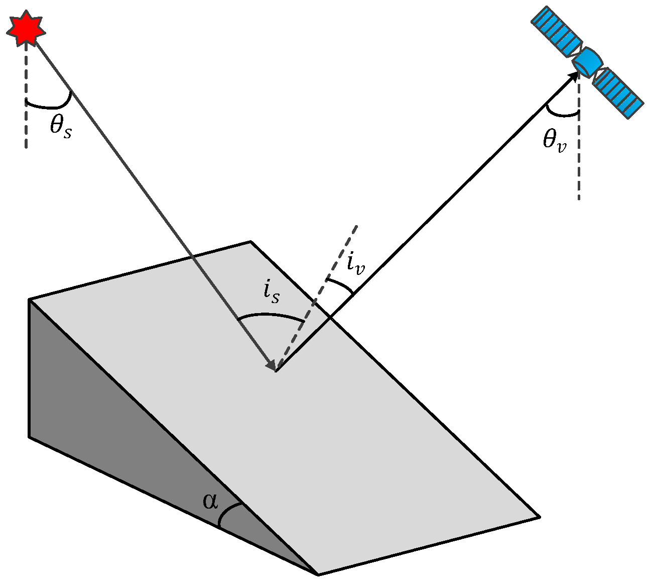
4.1. Physical Basis

The topographic effects on the solo slope BRDF depend on the slope and aspect angle, and the structural and optical properties of the vegetation. The surface’s slope and aspect change the local solar incidence and the sensor observation directions. Although vegetation shows crown geotropism, regardless of the terrain slope, its projection on the slope surface varies with the slope and aspect, and the direct and diffuse irradiance are redistributed. This changes the incident radiation received by the slope surface and the sensor observed radiation. Thus, the slope surface BRDF characteristics are distorted by the topography.

The solo slope BRDF model focuses on development of the slope changed radiation and accurate estimation of the 3D structure of vegetation and soil over the slope surface. Many physical BRDF models, such as the scattering by arbitrarily inclined leaves (SAIL) model [52], geometric-optical and radiative transfer (GORT) model [53], and forest reflectance and transmittance (FRT) model [54], as well as the computer simulation model of discrete anisotropic radiative transfer (DART) [38] and radiosity-graphics combined model (RGM) [55], have addressed the problems associated with solar radiation and complex 3-D canopy structure and background. The simulated BRF varied widely between these models under the activity provided by the radiative transfer model intercomparison (RAMI) [56], where a complex 3-D vegetation scenario is used as the benchmarking. However, the topography will introduce difficulty in the vegetation canopy anisotropic reflectance characterization. The reflectance anisotropy of the solo slope is the following function:

$$BRF=f({\Omega }_s,{\Omega }_v,DEM,para,ref,E)$$

(8)

where ${\Omega }_s$, ${\Omega }_v$, and DEM are the geometric parameters used to describe the anisotropic reflectance; $para$ indicates the canopy structure and land biophysical parameters, including crown height, crown density, crown shape, LAI, etc.; $ref$ represents the optical reflectance properties, such as leaf and background reflectance; and $E$ is the incident direct and diffuse irradiance.

Specifically, the topography alters the local solar incidence angle and the sensor observation geometry, as Figure 8 shows, which induces area changes in the canopy shadows cast on the background, as well as the mutual shadowing relationship between discrete heterogeneous tree crowns [21,57], photon path length within the homogeneous vegetation layer [20,27], and effective local illuminated slope irradiance [58]. Therefore, differences in terrain configuration significantly vary in reflected signals of surfaces with similar land cover, structural, and optical properties. A rotational transition matrix between horizontal coordinates and local slope coordinates is adopted to correct the geometric relationship.

$$\left[\begin{array}{c}\sin {\theta }_{is(v)}\cos {\varphi }_{is(v)}\\ \sin {\theta }_{is(v)}\sin {\varphi }_{is(v)}\\ \cos {\theta }_{is(v)}\end{array}\right]=\left[\begin{array}{ccc}\cos \alpha & 0& -\sin \alpha \\ 0& 1& 0\\ \sin \alpha & 0& \cos \alpha \end{array}\right]\left[\begin{array}{c}\sin {\theta }_{s(v)}\cos ({\varphi }_{s(v)}-\beta )\\ \sin {\theta }_{s(v)}\sin ({\varphi }_{s(v)}-\beta )\\ \cos {\theta }_{s(v)}\end{array}\right]$$

(9)

where $\theta$ and $\phi$ are the zenith and azimuth angles, respectively, the subscripts $is$ and $iv$ represent the local incident and observation geometries, and the subscripts $s$ and $v$ represent the incident and observation geometries.

However, the rotational geometric correction leads to crown inclination. This contradicts with the geotropic nature of tree crowns where the trees grow vertically and orient with the gravitational field, regardless of the slope. The crown structural and optical properties over the solo slope remain the same as those on the flat surface. For example, the leaf angle distribution (LAD) and leaf reflectance and transmittance reflectance are not affected by the terrain [27]. However, for the discrete forest stands, the crown shadowing projections on the background are influenced by the geotropic nature of tree crowns (as shown in Figure 9). The geometry correction using Equation (9) without negative geotropism consideration will lead to an incorrect crown shadowing (Figure 9b), as well as an inappropriate canopy reflectance. However, the tree crowns are virtually inclined after the geometric correction (Figure 9c). The importance of the geotropic nature of tree crowns has been stressed in the topographic correction of forested terrain [43,59].

Another topographic effect on the canopy reflectance is through the redistribution of surface global incident solar radiation, which modifies the upper boundary condition during the radiative transfer process. When compared to the flat terrain, the topography redistributes the direct solar irradiance by changing the surface’s local illumination and viewing geometry. The terrain restricts the diffuse skylight and enhances the diffuse irradiance that is reflected from adjacent slopes [25,59,60,61]. The last two diffuse components can account for 40% of the global radiation of a sunlit slope when the solar zenith angle is high, and this can even approach 100% when the slope is obstructed by adjacent terrains [46,62]. Moreover, varied elevation will induce rapid changes in concentrations of aerosol, water vapor, and cloud properties, which give rise to significant variations in the amount of direct and diffuse incident irradiance [63].

In the past decades, physical solo slope BRDF models have been proposed to account for the topographic effects on pixel reflectance. These are the BRDF models based on radiative transfer, geometric-optical, and hybrid methods (

Table 1. List of physical solo slope surface BRDF models.

Model Category	Model Name	Geometry Correction	Tree’s Negative Geotropism	Diffuse Irradiance	Typical Reference
Radiative transfer	ROSST	√	√	×	Combal et al. [27]
	PLC	√	√	√	Yin et al. [20]
Geometric optical	GOMST	√	×	×	Schaaf et al. [21]
	GOST1	√	√	×	Fan et al. [17]
Hybrid	SLCT	√	×	√	Mousivand et al. [64]
	GOST2	√	√	×	Fan et al. [24]
	GOSAILT	√	√	√	Wu et al. [65]

The symbols √ and × indicate that with and without consideration in the BRDF model, respectively. ROSST is the improved ROSS model for solo slope terrain; PLC is A Physical Solo Slope Canopy Reflectance Model Based On The Path Length Correction; GOMST is the geometric-optical mutual shadowing model for solo slope terrain; GOST is the 4-scale geometric-optical model for solo slope terrain; SLCT is the soil–leaf-canopy model for solo slope terrain; GOSAILT is the hybrid model of GOMS and scattering by arbitrarily inclined leaves (SAIL) coupled topography.

). Three key scientific issues include the geometry correction, negative geotropism of trees, and the irradiance redistribution, which affect the topographic BRDF. Since vegetation cover, such as forest and grassland, dominates the complex mountainous land ecosystem, current physical solo slope BRDF models mainly focus on the vegetation.

4.2. Model Development

4.2.1. Radiative Transfer Model

The radiative transfer process captures the vegetation canopy reflectance and further retrieves the vegetation physical and biophysical parameters, which treats the forest canopy as an homogeneous, turbid medium with discrete leaf elements [66]. The descriptions of leaf structural and optical characteristics, such as leaf size and shape, LAI, LAD, scattering phase function, and single scattering albedo, are key to this approach [53].

The importance of the topographic effect in the radiative transfer was first proposed by Combal et al. [27] who successfully extended the Ross radiative transfer theory [67] for flat plant canopies to solo slope with a vertical plant stand. The topographic effect on local geometry relationship has been considered in the ROSST model [27] through the transformation between horizontal and slope coordinate systems. The geotropic nature of tree crowns was accounted for by using the leaf structural and the optical characteristics defined in the horizontal coordinate to solving the one-dimensional (1-D) analytical radiative transfer equation. However, only the direct solar radiation was considered, the effect of diffuse skylight, path radiance, and diffuse irradiance from adjacent slopes are neglected. Recently, the topographic effect on the bidirectional gap probability has been regarded as the primarily factor affecting canopy reflectance [20,53,68]. A physical solo slope canopy reflectance model based on the path length correction (PLC) [20] was proposed to account for the topographic effect on the canopy photon path length and its BRDF. The geometry correction, geotropic nature of the tree crown, and the diffuse skylight are coupled in this model. However, the diffuse irradiance from neighboring terrains is still neglected.

4.2.2. Geometric-Optical Model

The geometric-optical model has an advantage in understanding the 3-D complex crown structure’s effects on the canopy reflectance [69,70], in which the pattern of sunlit and shaded crowns and backgrounds seen in a particular direction were considered to be the key factor. According to the geometric-optical theory, the canopy reflectance is assumed to be composed of four scene components: sunlit crown, sunlit background, shaded crown, and shaded background with their respective areal proportions.

The topographic effect on the canopy reflectance in the geometric-optical model was firstly evaluated by Schaaf et al. [21], who extended the Li-Strahler geometric-optical mutual shadowing model for a solo slope surface (GOMST) through a simple geometry correction, while retaining other structural and optical properties the same as those in the horizontal forest. The accurate estimation of the topographic effect on the crown cast shadow for the background is critical for canopy reflectance. When a slope faces toward the sun, less crown shadows are projected on the background, and more shadows are cast on the background when it is away from the sun [18,57]. The trees are assumed to be perpendicular to the solo slope without negative geotropism in the GOMST model, which will lead to an underestimation in the red reflectance. This is because the areal proportion of the background will be underestimated, while the areal proportion of the crown will be overestimated in this case. However, the canopy reflectance and albedo also appear to be significantly affected by terrain even without consideration of the trees’ negative geotropism [21]. Fan et al. [17] incorporated the topographic effect into the 4-scale geometric-optical model for solo slope terrain (GOST1), which acknowledged the geotropic nature of tree crowns. However, the diffuse irradiance components are neglected in the current geometric-optical models, which will cause an underestimation of global incident irradiance and surface reflected signals.

4.2.3. Hybrid Model

The radiative transfer model is accurate in estimating the canopy reflectance with micro-scale leaf reflectance, especially for high orders of scattering and diffuse irradiance effects, and the geometric-optical model is accurate in describing the single scattering results from 3-D forest crown structure. Thus, hybrid models that combine the two approaches can capture discontinuous canopy reflectance at the landscape scale [52,53,71].

In mountainous regions, the GOST1 model was coupled with the recollision probability theory to parameterize the component reflectivity, which is called the GOST2 model [24]. The multiple scattering within canopy-background system is considered in the GOST2 model. However, GOST2 reflectance seems to be overestimated. The main reason might be that a fixed relationship between the canopy structural parameters, LAI and photon recollision probability was implemented in the GOST2 model. Like the GOST1 model, the diffuse irradiance components are neglected in the GOST2 model. The soil–leaf-canopy (SLC) model has successfully captured discontinuous canopy reflectance through incorporating the crown clumping effects, vertical leaf color gradient, and non-Lambertian soil background into the scattering by arbitrarily inclined leaves (SAIL) model [52]. It has been extended to the solo slope surface (SLCT) by simply applying the geometric correction without consideration of the geotropic nature of the tree crowns [64]. Therefore, the red and NIR reflectance of the SLCT model were underestimated and overestimated, respectively. Similar to SLCT, GOMST was recently extended by the SAIL model and coupled topography (GOSAILT), for sloping forest, where the effects of slope, aspect, geotropism of the tree crown, multiple scattering scheme, and diffuse skylight are considered [65]. This avoids the issues of reflectance simulation being underestimated and overestimated over rugged terrain.

The computation simulation model can be treated the same as the hybrid model since it can accurately simulate canopy reflectance for both continuous and discontinuous forest stands [38]. Currently, the Monte Carlo ray-tracing (MCRT) computational models have been modified for the solo slope through a coupling of the surface’s complex topography by importing the digital elevation model (DEM) datasets or a bilinear surface interpolation based on some simple terrain parameters [38,72]. When compared with the flat terrain, the simulations for rugged mountainous regions face a greater burden of huge memory requirement and computational loading, especially for complex terrain with large maximum elevation differences or large scenes [73].

4.3. Topographic Effect on Solo Slope BRDF

According to the solo slope BRDF simulated results from previous studies, we can conclude that the hotspot still occurs in the solar direction, regardless of slope when the canopy is located on a solo slope terrain. However, the magnitude and shape of BRDF shows an almost random difference caused by shadowing patterns, and the local illumination angle varies with the slope elevation and aspect almost randomly [20,21,57]. For example, as shown in Figure 10, when compared to a flat canopy illuminated by the north solar angle, the slope increases the canopy red reflectance in the backward direction and decreases the red reflectance in the forward direction relative to the solar incidence, respectively. However, The canopy NIR BRDF shape over a steep slope (60°) is distorted, especially in the forward direction, which is where the reflectance is higher than that in backward direction (Figure 10f) [21]. However, the slope seems to have no effect on the canopy reflectance in the direction perpendicular to the aspect of the solo slope terrain because the path length remains constant in the nadir direction due to the geotropic nature [20]. The skewed BRDF in the hemisphere leads to a distinct variation in the albedo values. When compared to the slope angle, the surface albedo is more sensitive to the aspect over the steep slopes. In particular, a larger albedo occurs for the slope facing away from the sun than the sunward facing slope due to the increasing local solar zenith angle and mutual shadowing.

5. Composite Slope BRDF Model

5.1. Physical Basis

The composite slope terrain, which is composed of many micro-sloping terrains within one pixel, is shown in Figure 11. For the composite sloping terrain, the topographic effects on reflectance are generally focused on the integrated effects of the micro-slopes within one remote sensing pixel, and they ignore the effects at the pixel level [29,74]. The micro-slope terrain variabilities lead to the shadows coming from both self-shadowing and shadows from the surrounding topography, and this alters the distribution of the composite slope incident radiation. Different spatial distribution characteristics of the micro-topography lead to different spatial geometric configurations of sun-sub-terrain-sensor, multi-scattering, and obstructing effects within the pixel. Characterizing and parameterizing the spatial distributions of the micro-slope topographic features are the key to modeling the BRDF over the composite slope terrain.

The anisotropy reflectance $BR{F}_{coarse}$ of the composite slope terrain has the following functional form:

$$BR{F}_{coarse}=f({\Omega }_s,{\Omega }_v,DE{M}_{fine},BR{F}_{fine})$$

(10)

where $BR{F}_{fine}$ is the bidirectional reflectance of the micro-slope, which can be calculated with the BRDF models of the solo slope. $DE{M}_{fine}$ represents the fine scale digital elevation models compared with the composite terrain.

Specifically, according to the principle of geometric optics and radiosity [75], under the assumption of a horizontal composite slope surface, its directional reflectance is as follows:

$$BR{F}_{coarse}=\frac{{\displaystyle \underset{A(s,v)}{\int }\cos i_{sj}BR{F}_{fine}(i_{sj},i_{vj},{\varphi }_{sj},{\varphi }_{vj})\cos i_{vj}d{A}_{tj}}}{\cos {\theta }_s{\displaystyle \underset{A(v)}{\int }\cos i_{vj}d{A}_{tj}}}$$

(11)

where the subscript $tj$ is the $j$th micro-slope; $A_{tj}$ denotes the incremental surface area of the micro-slope; $i_{sj}$, $i_{vj}$, ${\phi }_{sj}$, and ${\phi }_{vj}$ are the relative solar zenith angle, relative sensor zenith angle, relative solar azimuth angle, and relative sensor azimuth angle, respectively, which correspond to the micro-slope; ${\theta }_s$ and ${\theta }_v$ are the solar zenith angle and sensor zenith angle, which correspond to the horizontal plane; $A(s,v)$ denotes the micro-slopes that are both illuminated and visible; and, $A(v)$ denotes the visible micro-slopes.

From Equation (11), it can be concluded that BRDF modeling over the composite slope terrain is an inherently upscaling procedure. In addition to the effects of the micro-surface slope and aspect, the shadowing distribution within the composite slope is also identified as an essential factor to account for the topographic effects on BRDF. The amount and distribution characteristics of the shadow have great effects on the surface BRDF [76]. The shadowing function (also called the geometric attenuation factor) is built to describe the shadowing and masking effect [30,77,78,79,80]. Models are used to describe the complex upscaling process by combining the shadowing function $S$ and an equivalent reflectance $BR{F}_{eq}$, which neglect the shadowing effect. In this case, the BRDF over the composite slope terrain can be written as follows:

$$BR{F}_{coarse}=BR{F}_{eq}\times S({\Omega }_s,{\Omega }_v,DE{M}_{fine})$$

(12)

Essentially, the composite slope BRDF depends on the distribution characteristics of the interior topography of the remote sensing pixels. From the description of the topographic characteristics, BRDF models over the composite slope terrain can be divided into the special-shape based model, random field based model, and real DEM based model (

Table 2. Overview of composite slope BRDF models.

Type	Terrain Description	Interior Topography Characteristics	Typical Reference
Special-shape	V-cavity	The surface consists of small symmetrical or non-symmetrical V-cavities	Torrance et al. [79]; Liu et al. [81]; Blinn et al. [82]
	Sphere-cavity	The surface consists of periodical positive sphere-cavities or negative sphere-cavities.	Buhlet al. [83]; Poulin et al. [84]; Koenderink et al. [85]
Random field	Random distribution	The height or the slope conforms to the Gaussian normal distribution, the exponential distribution, or other random distributions	Despan et al. [77]; Hapke [80]; Brockelman et al. [86]; Smith [87]
	Fractal	Describes the dependence of surface roughness on scale by a power law	Barsky et al. [78]; Shepard et al. [88]
DEM	DEM	The terrain is described by high spatial resolution digital elevation models	Wen et al. [29]; Roupioz et al. [31]

).

5.2. Model Development

5.2.1. Special-Shape Based Model

A simple and effective method used to characterize the topographic effects on BRDF is to take the terrain surface as a special-shape to model the surface anisotropic reflectance. Specifically, the composite slope surface is assumed to be composed of several elements with a repeated primitive shape, such as the V-cavities and spherical-cavities, which are shown in Figure 12. For the V-cavities, the distribution of the slope angle with respect to the horizontal plane is used to describe the surface roughness [78]. Positive sphere-cavities and negative sphere-cavities are the two types of terrain configurations, as shown in Figure 12b,c. The depth-to-diameter ratio of each spherical-cavity [79] and the distance between the centers of the two adjacent spherical-cavities [81] are the two main parameters used to describe the surface roughness. Although the actual terrain shape is probably much more complex, because it consists of various oriented micro-slopes, to describe the topographic relief and its shadow, a spherical or V geometry represents a reasonable physical approximation and mathematical treatment.

For V-cavities, when considering the effects of shadowing and masking of facets by adjacent facets, the T-S model [79] first took this terrain configuration and further introduced a simplified, piecewise trigonometric function [82] to improve the qualification of shadowing effects. Although V-cavities have a simple configuration, the model assumes that adjacent micro-slopes have the same slope angle with opposite orientations, which will result in sharp, abnormal turning points in BRDF curves [81]. Therefore, by assuming that adjacent micro-slopes are oriented in opposing directions, but not symmetrical and the slope angle of each micro-slope follows a semi-Gaussian distribution, an improved anisotropic reflection model was developed, which is closer to the natural configuration of the topography. The results showed that this model reached better physical rationality and improved the accuracy of the BRDF model [81]. However, it would be difficult to elaborate an analytical model coupled with the multi-scattering component over the composite slope terrain. Although a simple and physically plausible construction is proposed for the multi-scattering effect and is coupled with the single reflection in the research by Kelemen et al. [89], the multi-scattering effect is usually neglected or handled as a constant diffuse factor, which is against practical observations [90].

The positive spherical cavities allow for large grooves with relatively sharp edges that are better than the V-cavities [83]. The negative spherical cavities can approximately depict a rough surface, like the small craters on the moon [84]. Buhl et al. (1968) [83] first assumed the rough surface to be a collection of positive spherical cavities, but did not present a complete mechanism that accounts for masking and shadowing effects for arbitrary incidence and exit. Following this, analytical anisotropic reflection models for positive sphere-cavities and negative sphere-cavities were derived [84], which take into account hiding and shadowing between spherical cavities and can be easily implemented. An algebraic solution for multi-scattering in the spherical cavity was further provided and confirmed that the exact (numerical) calculations for a spherical geometrical surface, coupled with the multi-scattering effect are physically realizable [85].

5.2.2. Random Field Based Model

While the hypothesis of V-cavities or sphere-cavities is appropriate mathematically, it is not physically plausible. The terrain surface is far from the V-cavities or spherical cavities. More complex and realistic configurations for the topography description are the random field, which include the fractal characteristics [91,92], exponential distributions [45,93,94], Laplace distribution [94], and Gaussian normal distribution [3,95]. These are widely applied in early quantitative mathematic reflectance models over the random rough surface [96] in optical engineering, radiophysics, metrology, computer graphics, and machine vision fields. Remote sensing scientists have developed a series of anisotropic reflectance models based on the random field, especially when it was assumed that the micro-slope distribution follows a random Gaussian distribution and self-affine fractals. For the surface with a Gaussian random distribution, the root mean square (RMS) slope [87], correlation length [87], and mean slope angle [30] are adopted to parameterize the characteristics of the random surface. For the surface with self-affine fractal characteristics, the Hurst exponent is the key to determining the roughness features. Figure 13 shows the rough surface with a typical, random normal distribution.

Initially, a series of shadowing functions have been developed over one-dimensional surfaces with a Gaussian random distribution to describe the interior topographic effects on the surface anisotropic reflectance. The first attempt of analytical derivation of the shadowing function can be traced back to the work of Beckmann [97] who derived the Beckmann shadowing function, which uses a Gaussian correlation function to characterize the random surface. However, it does not agree well with the numerical simulation [86] because of a mathematical error in the model derivation [98]. A rigorous shadowing function expression based on the surface with a Gaussian height field was presented by Wagner [99]. The Wagner shadowing function adopted integral approximations and ignored the correlation between the height of the rough surface and its slope, which leads to large analytical complexity. The Smith shadowing function further improved the Wagner shadowing function by introducing a normalization function and simplified the calculation complexity [87].

Heitz et al. (2016) [100] extended the Smith model to include micro-surface multiple scattering at rough material interfaces, which agree well with the computer simulation. However, these shadowing functions assume that the joint probability density of the random surface heights and slopes is uncorrelated. The effects on the Wagner and Smith shadowing functions were quantified and showed that they have large errors when the incidence angle is large because the real-world continuous surfaces have wider autocorrelation functions [101].

Extending the one-dimensional model to a two-dimension model is another important way to derive a shadow function [102], such as the Hapke shadowing function [80] and the Despan shadowing function [77]. The Hapke shadowing function is derived from the radiative transfer process and the raw equivalent slope principle. This function accounts for any general configuration of incidence, emission, and azimuth angles on the two-dimensional (2-D) surface [80], which involves only one arbitrary parameter of the mean slope angle. The Despan shadowing function was derived by using rigorous probabilistic techniques, including a conditional probabilistic distribution and total expectation formula [77], where the random rough surface is described as an isotropic 2-D Gaussian stochastic process with a Gaussian autocorrelation function.

Self-affine fractals are another way to describe natural surfaces [88]. They describe the dependence of surface roughness on scale by a power law. Shepard and Campbell (1999) first proposed an empirical formula for the fractal shadowing function, but no rigorous analytical models of self-shadowing on a fractal surface currently exist [88]. Further, an analytical integral form of the shadowing function for fractal surfaces with different fractal and roughness parameters [78] was offered and opens possibilities for further exploration of fractal surfaces behavior. An agreement was demonstrated between the fractal model and experimentally calculated shadowing functions using the Monte Carlo method.

5.2.3. DEM-Based Model

Random field models are usually constructed based on rigorous probabilistic techniques. Thus, in general, the random field of Gaussian normal distribution or other statistical distribution regarding the terrain is acknowledged at a large scale (more than 10 km). However, the real terrain surfaces often exhibit non-random spatial distribution characteristics at a relatively small scale (such as a 1 km remote sensing pixel). Investigations have shown the sub-terrain slope distributions within each kilometric pixel of more than 50% over the Tibetan Plateau is not normal [31]. It is questionable to directly apply the random field hypothesis to remote sensing BRDF modeling at a kilometer scale. Recently, accurate digital elevation models (DEM), such as GDEM2 [103] have become available at a global scale with a 30-m spatial resolution. These DEMs offer an efficient way to describe the surface topography. Rapid and accurate methods for calculating slope and azimuth, solar illumination angle, shadow factor, and sky view factors have been proposed [104]. These methods prompt us to model the BRDF by considering the micro-topographic effects based on the DEM.

According to the radiosity theory [75], a physical BRDF upscaling model based on Equation (11) and the multi-scattering consideration for sub-topographic effects [31] was developed. However, this procedure requires the micro-slope surface BRDF and topographic factors, which leads to complexity and low computational efficiency. Similarly to mean slope derived from the random field, the equivalent slope model (ESM)was proposed to derive the equivalent slope and aspect [29] to simplify this process. This model assumes that there is a virtual smooth slope where the incoming and outgoing radiation are the same as that of the composite sloping terrain and this is related to the position of the sun, sensor and micro-surface slope and aspect of the DEM, which is shown in Figure 14. Thus, ESM can account for the effects of the sub-topography and shadow distribution. Similar to the shadow function, a sub-topographic impact factor $T$ can be derived from the equivalent slope. Therefore, $BR{F}_{coarse}$ can be expressed as a function of anisotropic reflectance $BR{F}_{eq}$ of the equivalent slope and the sub-topographic impact factor $T$:

$$BR{F}_{coarse}=BR{F}_{eq}\times T({\Omega }_s,{\Omega }_v,DE{M}_{fine})$$

(13)

where $BR{F}_{eq}$ can be obtained by the solo slope BRDF models, and $T$ is written as follows:

$$T({\Omega }_s,{\Omega }_v,DE{M}_{fine})=\frac{\cos i_v^{e}cso{i}_s^e{\displaystyle \underset{A(s,v)}{\int }d{A}_{tj}}}{\cos ({\theta }_s){\displaystyle \underset{A(v)}{\int }\cos i{v}_{j}d{A}_{tj}}}$$

(14)

where $i_s^e$, $i_v^e$, ${\phi }_s^e$, and ${\phi }_v^e$ are the relative solar zenith angle, relative sensor zenith angle, relative solar azimuth angle, and relative sensor azimuth angle, respectively, which correspond to the equivalent slope.

When compared with the Hapke shadowing function $S$, which represents the amount of shadow on the composite slope, the sub-topographic impact factor $T$ represents the effects of the tilted micro-slope distribution and mutual shadowing. For example, when the solar zenith angle is 0°, $S$ is one regardless of the sensor zenith angles and mean slopes. This is because there is no shadow when the sun is at nadir. However, $T$ is smaller than 1 when the mean slope is large and changes slightly with the view zenith angle when the solar zenith angle is 0°. When the solar zenith angle is 45°, both of these values are less than one [29].

5.3. Topographic Effect on Composite Slope BRDF

The magnitude and shape of BRDF over composite sloping terrain shows significant changes in response to the altered topography, which is because of the nonlinear dependence of BRDF on the micro-slope spatial configuration [29,76,105]. An asymmetric distributions of BRDF can be observed because of the shadow effects and the adaption of the sun-terrain-sensor geometry [29,72,105]. However, the BRDF peak location over the composite slope terrain is identical to that over flat terrain [72]. With the same sun and sensor directions, the deviation between the reflectance over composite slope terrain and that over flat terrain is sensitive to the mean slope. The deviation cannot be neglected even when the mean slope is small [36]. The deviation increases gradually with an increased mean slope, and it reaches 80% at about 37° of the mean slope when the SZA and VZA are around 60° [29]. The lowest deviations are found for the sun at zenith, and they increase considerably with an increase in SZA. Generally, there is a larger reflectance value when the VZA is larger. It also depends on the VAA and decreases when the viewing direction changes from the principal plane to the perpendicular principal plane [36].

6. Future Development and Perspective on BRDF Products Generation

Accurately generating a BRDF product over rugged terrain at the global scale is crucial for vegetation monitoring, as well as the energy budget for global climate change research. Various BRDF forward models have been developed to fit and explore the topographic effects of BRDF over rugged terrain. Because of a lack of operational algorithms for the BRDF product over rugged terrain, the current BRDF products do not account for the topographic effects, and thus, they show large uncertainties. According to the key steps of BRDF modeling, users should choose a high quality DEM and fast parameterization methods to obtain topographic factors. To extend the forward BRDF model to the operational one, it is necessary to adopt new and innovative ideas to overcome the limitations of BRDF applicability over rugged terrain, and to develop an effective method for validating the BRDF algorithm and satellite product performance.

6.1. High Quality DEM

The availability of high quality DEMs promotes the development of BRDF modeling over rugged terrain. In recent years, stereo photogrammetry and interferometric synthetic aperture radar techniques have been widely used to generate DEMs, as well as providing fast, reliable, and accurate solutions. Accurate DEM products are available at a global scale with resolutions of up to 30 m, which include GTOPO30 DEM, SRTM3DEM, SRTM CGIAR-CSI DEM, TanDEM-X DEM, ASTER GDEM1, and ASTERGDEM2.

The BRDF models of solo slope, composite slope, and the sloping reflectance retrieval show that their accuracies depends on the quality of the calculated topographic terms from the DEM. The issues of elevation accuracy, spatial resolution, and the co-registration accuracy between the DEM and satellite image are easy to identify but difficult to assess. Geo-location errors, elevation aberrations, and even blunders in the DEM base data can result in significant local errors in BRDF modeling. A high quality DEM is the basic necessity prior to successful BRDF modeling over rugged terrain. An external validation showed that the elevation accuracy of ASTERGDEM2 is 8.5 m and that of SRTM3 USGS is 6 m [103]. The precision of the DEM enables us to apply the observed correlation between shading and images [106] to improve the co-registration accuracy. DEM spatial resolution is another factor that should be considered in modeling the BRDF over rugged terrain. A low resolution DEM when compared to the remote sensing pixel will not provide detailed topographic information because the DEM resolution changes [107,108,109], mean slopes and curvatures decrease, and terrain details disappear. Thus, a scale appropriate for the satellite data is of great importance in BRDF modeling. We suggest that a high quality and high spatial resolution DEM is necessary for BRDF modeling based on both high resolution and low resolution remote sensing images, which correspond to the solo slope BRDF modeling and composite slope modeling, respectively.

6.2. Topographic Factor Parameterization

Because the DEM describes 3-D surface, several parameters to characterize landforms and surface-received solar radiation can be extracted from DEM datasets, and consequently, these can be used in the BRDF models. These include the slope and aspect describing the topography gradient and orientation, the topographic shadow mask indicating whether the target surfaces are sunlit, the sky view factor representing the proportion of the sky visible to the target surface, and the topographic configuration factor, illustrating the proportion of target slopes that are visible to the surrounding slopes [104]. All of these parameters are regional properties because their calculations depend on a suitable neighboring area. Although a formidable computational problem occurs during the calculation of these parameters, they require calculation only once, and thus, they can be stored as look up tables (LUT) before the actual model execution due to their stationary property, especially for deriving global products.

Specifically, the calculation of the slope and aspect of the target slope depends on the gradients in the east-west and north-south directions [110]. A moving 3 × 3 window is commonly used to derive the gradients. According to the pixels in the window adopted to calculate the gradients and their respective weights, six slope and aspect algorithms are frequently used. These algorithms include second-order finite difference [111,112], third-order finite difference [113,114], third-order finite difference weighted by reciprocal of squared distance [113], third-order finite difference weighted by reciprocal of distance [115], frame finite difference [116], and simple difference [117]. The algorithm for the topographic shadow mask indicates whether the slope is shadowed by the neighboring slope from the solar direction. The global decision tree [31], minimum radius search [118], and indirect horizontal angle [104] algorithms are the three frequently used methods. The sky view factor is defined as the ratio of the diffuse skylight that is received by the target slope to an unobstructed horizontal surface [104]. This value is restricted between 0 and 1. Values close to 1 indicate that the point is located at the top of the topography, and values that reach 0 indicate the point lies in the low part of a deep valley. This factor accounts for the slope and aspect, the obstruction from neighboring slopes, and the anisotropy of diffuse skylight. However, the anisotropic diffuse skylight is always neglected in the current sky view factor algorithm. Several algorithms have been proposed depending on whether the neighboring topographic obstruction effect is considered or the horizontal or inclined slope are taken as a reference [104,119,120,121]. Similar to the sky view factor, the topographic configuration factor is defined as the ratio of the nearby slope reflected irradiance received by the target slope on an unobstructed horizontal surface [104]. Directly calculating the topographic configuration factor is difficult, since the reflected irradiance of every slope facet visible to the target slope needs to be known. The alternative solution for the topographic configuration factor is that it can be expressed as the difference between the sky proportion for an infinite slope and the actual slope sky view factor [104,120].

6.3. Potential Method to Derive the BRDF Product over Rugged Terrain

Since the solo slope and composite slope BRDF models in this study are forward BRDF models, it is not possible to use these models as the BRDF operational algorithm to generate the BRDFs. The current linear kernel-driven model has been successfully adopted to derive the satellite BRDF/albedo products because of its simplicity, feasibility, and physical basis [122,123]. There has been no significant further progress in the kernel-driven model to fit the BRDF with multi-spectral and multi-angular reflectance. However, the effects of topography are rarely coupled in the kernel-driven models, which leads to uncertainties in the BRDF/albedo retrieval over mountainous areas [9,19]. Thus, a suitable forward BRDF model to derive the kernel function coupled with topographic effects is necessary to generate the BRDF product at the global scale.

As for the solo slope surface, most of the forward BRDF models cannot be directly derived with the kernel functions due to its complicated physical processes. Therefore, the current kernel driven models that are applied in mountainous areas are modified by a geometric relationships transformation between the horizontal surface and sloping plane. Specifically, this transform changes the solar and sensor view angles corresponding to the slope surface in the kernel function to reflect the sloping surface effects. Because of the shadow that is caused by the topography obstruction, the diffuse skylight serves as the dominant illumination energy source. Then, the kernel function derived from the BRDF model may be a constant according to a geometric-optical model, where the component spectral contrasts are neglected when the pure diffuse surface scatters. However, the spectral signatures of the scene components still show distinct difference even under the pure diffuse skylight illumination [71]. This may also be described by the hemispherical directional reflectance factor (HDRF, [8]) and the pixel HDRF displays an angular heterogeneity [8,124,125]. For the composite slope surface, the coarse-scale pixel directional reflectance is affected by the micro-slope internal to the pixel, in addition to the 3-D object structure itself, which includes the proportion of shadow, and micro-surface slope and aspect distribution. However, the current kernel driven model is applied directly to mountainous areas under the assumption that the topographic relief is a special 3-D object. The accuracy and uncertainties of this model are not yet credible and should be further evaluated. One of the deficiencies in the current kernel driven function is that it neglects topographic effects, which results in no topographic factors being included in the kernel function.

Therefore, a possible solution is to derive a united kernel driven function suitable for both solo-slope and composite-slope surfaces. According to the current BRDF model developed over rugged terrain, GOSAILT can be further derived as the solo slope kernel function, which is then is coupled with a sub-topography impact factor of the equivalent slope model (ESM) to form the composite slope kernel function. The ESM can extend the solo slope BRDF to the composite slope BRDF. The most important feature of these two models is that they are forwarded based on a real DEM, which will enable us to further promote the possibility of a united kernel function. Specifically, GOSAILT can be implemented to derive the linear semi-empirical kernel-driven model that is suitable for sloping terrains under both clear and overcast skies; this model has a similar framework to the RossThick-LiSparse Reciprocal (RTLSR) BRDF model [9], which includes sloped geometric-optical and volume scattering kernels. The ESM, an anisotropic reflectance model over the composite sloping terrain, was developed based on the equivalent slope principle. It extends the directional reflectance model for the solo sloping terrain to the reflectance model for the composite sloping terrain by a sub-topography impact factor, which describes the topographic influence. Similar to BRDF extension, by coupling with the sub-topography impact factor, the GOSAILT kernel function can be easily applied to the BRDF retrieval over rugged terrain.

Progress is also expected in the retrieval method development, which uses data from combined multi-sensors in mountainous areas. Low quality and cloud occlusion causes remote sensing data unavailability in mountainous areas to be more severe. Thus, the significant merit of combining multi-sensor reflectance is that it can provide additional multiple angular information, and then, this can improve the inversion accuracy of the BRDF on mountainous surfaces. For example, the multi-angular and multi-spectral kernel function (ASK) model [126,127] and multi-sensors combined BRDF inversion (MCBI) model [128] are proposed from the improvement of the BRDF kernel function, as well as the need to retrieve the BRDF synthetically by combined multiple sensor reflectance, which has a continuous spatial distribution and shorter-time scale of BRDFs.

Lastly, the remaining difficulties include the fast extraction of the DEM topographic factor and the support of the kernel function to fit the BRDF over rugged terrain. The look up table (LUT) might be a practical method to store all of the topographic factors, including slope, aspect, and shadow, as well as the sub-terrain impact factor with the different solar SZA, SAA, and DEM longitude and latitude. When the sloped kernel driven model is implemented, the global shadow, observing mast, sky view factor, topographic configuration factor, and ESM LUT provide the essential parameters that are needed to produce global BRDFs. For example, the SZA is from 0° to 65° with an interval 5°, and the SAA is from 0° to 330° with an interval 30° in the global topographic shadow mask (TSM) LUT. Figure 15 is the global topographic shadow mask, where the SZA is 40° and SAA is 0°.

6.4. Validation Methods for the BRDF over Rugged Terrain

In situ multi-angular reflectance data, which is measured at sites with typical, homogeneous surfaces, is the ground reference truth for the land surface BRDF validation. However, the BRDF validation dataset is still far from sufficient to support the global BRDF validation, which is mainly due to the limitations of multi angle observation instruments and technique developments.

In mountainous areas, the BRDF measurement can be more difficult than those on flat surfaces due to the slope effects. First, there is still some controversy regarding the measurement method of the sloped BRDF. For example, whether the observation instrument should be parallel to the slope surface or the horizontal surface is a question that needs to be answered according the definition of the modeled BRDF. Second, mountainous area generally belongs to the forest land type, where the tree height might be too high for users to reach. It is difficult to carry out multi-angular forest canopy reflectance measurements with ground based instruments. One of the alternative methods is to use a tower to implement the multi-angular measurements, where the height of the tower should be higher than that of the forest canopy. Another alternative is the use of unmanned aerial vehicle (UAV) technology. A UAV can carry the optical CCD and provide multi-angular reflectance measurements for a small-scale area. The tower-based or UAV-based measurements only represent the scale of the solo slope. To validate the BRDF over the composite slope surface, a multi-scale validation strategy is important to solve the spatial scale mismatch between the ground-based and the satellite-based BRDF. However, the technique for BRDF upscaling over rugged terrain is still an ongoing subject of research, which has limited the applicability of the multi-scale validation strategy.

A current alternative validation method, especially for the BRDF validation of the composite-slope, is generally based on computer simulation technology [38,73,129], or the use of a miniature terrain sandbox to simulate the BRDF under the influence of topography as the reference truth. Computer simulation technology, such as discrete anisotropic radiative transfer (DART) [38], can set up different DEMs and different types of trees to build a real scene of solo slope or composite slope forest over rugged terrain. With the flux tracing technique, the multi-angular reflectance reference dataset is simulated. The terrain sandbox can simulate different typical composite terrains, as well as the different vegetation above the terrain. With the help of existing imaging spectroscopy technology, the multi-angular observation can be implemented to obtain the reference reflectance dataset.

7. Conclusions

In this paper, the model of bidirectional reflectance distribution function (BRDF) over rugged terrain has been comprehensively reviewed. The results of the literature analysis demonstrate that the subject of BRDF modeling over rugged terrain has been intensively addressed by remote sensing scientists over the past ten years. Referencing the BRDF definition, we proposed two kinds of BRDF over rugged terrain, according to the relationship between the spatial resolution of the DEM and remote sensing image pixel. These are the solo slope BRDF and the composite slope BRDF. Their scale difference and their self-consistencies should be emphasized.

The dominant factors of the BRDF over the solo slope and composite slope are different. The surface slope and aspect of the pixel level, which change the sun-terrain-sensor geometry, as well as the radiation distribution, are the factors controlling the solo slope BRDF. However, with the composite slope BRDF, besides the influence of the micro-slope within the pixel, the influencing factors are also the shadow distribution of the terrain occlusion, overall distribution of the micro-terrain, and the multiple scattering between micro-slopes. These sensitive factors should be concentrated on when modeling the BRDF over these two kinds of slopes.

Specifically, an accurate description of the interaction between the 3-D vegetation structure, soil, and atmosphere is of great importance for solo slope BRDF modeling. Radiative transfer, geometric-optical, and the hybrid theory are the three basic theories that are used to mathematically solve the interaction process. The geotropic nature of tree crowns and accurate parameterization of the components radiation signal of vegetation and soil in the solo slope BRDF modeling is important. However, the description of the sub-topographic effects is the critical step for composite slope BRDF modeling, which is where the virtual random distributed topography and real DEM are the two solutions for the description of sub-topography inside the coarse scale pixels. The shadow function and the sub-topography impact factor are the two parameterizations. The sub-topography impact factor can be linked to the solo slope BRDF and the composite slope BRDF, where they both are based on the real DEM. When compared with the solo slope BRDF model, the development of a composite slope BRDF model should be further researched based on the simulated data and to achieve better accuracy.

According to the current BRDF model over rugged terrain, it is concluded that the topography can intensely affect both the shape and magnitude of the land surface BRDF. Generally, when a slope increases of the solo slope surface, the canopy reflectance opposite to the solar direction also increased, but the reflectance in the forward to solar direction decreased, which resulted in a skewed BRDF in the hemisphere. Thus, this consequently led to a distinct variation in the albedo values, as well as other parameters that are derived from the land surface BRDF. However, the hotspot direction and the solar orthogonal plane to the aspect of the solo slope terrain seem to have less topographic effects on the canopy reflectance. The composite slope surface, shadow, and sub-terrain slope result in asymmetric distributions of BRDF. The BRDF shape and magnitude depends on the mean slope, the dominated aspect of sub-terrain, the SZA, and SAA. With the mean slope increased, the topographic effects of BRDF are more intense under the same sun and sensor location. Even in the case of a relatively smaller mean slope, the deviation between the reflectance over composite sloping terrain and that over flat terrain is still significant.

Although relatively high quality DEMs are available, and the topographic factors can be parameterized quickly, it seems that the operational BRDF model used to fit the remote sensing satellite multi-angular reflectance does not show significant progress. Similar to the kernel driven model used in the MODISBRDF/albedo product, the kernel functions derived from the current forward BRDF model over rugged terrain are still a subject for ongoing research. Although GOSAILT seems to be able to derive the kernel function of the solo slope and composite slope, more efforts should be put toward operational BRDF model development and its validation over rugged terrain.

References

1. Li, A.; Jiang, J.; Bian, J.; Deng, W. Combining the matter element model with the associated function of probability transformation for multi-source remote sensing data classification in mountainous regions. ISPRS J. Photogramm. Remote Sens. 2012, 67, 80–92. [Google Scholar] [CrossRef]
2. Vanonckelen, S.; Lhermitte, S.; Rompaey, A.V. The effect of atmospheric and topographic correction methods on land cover classification accuracy. Int. J. Appl. Earth Obs. Geoinf. 2013, 24, 9–21. [Google Scholar] [CrossRef]
3. Helbig, N.; Löwe, H. Shortwave radiation parameterization scheme for subgrid topography. J. Geophys. Res. Atmos. 2012, 117, 812–819. [Google Scholar] [CrossRef]
4. Wen, J.; Zhao, X.; Liu, Q.; Tang, Y.; Dou, B. An improved land-surface albedo algorithm with DEM in rugged terrain. IEEE Geosci. Remote Sens. Lett. 2013, 11, 883–887. [Google Scholar]
5. Yan, G.; Wang, T.; Jiao, Z.; Mu, X.; Zhao, J.; Chen, L. Topographic radiation modeling and spatial scaling of clear-sky land surface longwave radiation over rugged terrain. Remote Sens. Environ. 2016, 172, 15–27. [Google Scholar] [CrossRef]
6. Pasolli, L.; Asam, S.; Castelli, M.; Bruzzone, L.; Wohlfahrt, G.; Zebisch, M.; Notarnicola, C. Retrieval of leaf area index in mountain grasslands in the alps from MODIS satellite imagery. Remote Sens. Environ. 2015, 165, 159–174. [Google Scholar] [CrossRef]
7. Zhao, P.; Fan, W.; Liu, Y.; Mu, X.; Xu, X.; Peng, J. Study of the remote sensing model of FAPAR over rugged terrains. Remote Sens. 2016, 8, 309. [Google Scholar] [CrossRef]
8. Schaepman-Strub, G.; Schaepman, M.E.; Painter, T.H.; Dangel, S.; Martonchik, J.V. Reflectance quantities in optical remote sensing—Definitions and case studies. Remote Sens. Environ. 2006, 103, 27–42. [Google Scholar] [CrossRef]
9. Gao, F.; Schaaf, C.B.; Strahler, A.H.; Jin, Y.; Li, X. Detecting vegetation structure using a kernel-based BRDF model. Remote Sens. Environ. 2003, 86, 198–205. [Google Scholar] [CrossRef]
10. Schaaf, C.B.; Gao, F.; Strahler, A.H.; Lucht, W.; Li, X.; Tsang, T.; Strugnell, N.C.; Zhang, X.; Jin, Y.; Muller, J.-P. First operational BRDF, albedo nadir reflectance products from MODIS. Remote Sens. Environ. 2002, 83, 135–148. [Google Scholar] [CrossRef]
11. Xiao, Z.; Liang, S.; Wang, J.; Jiang, B.; Li, X. Real-time retrieval of leaf area index from MODIS time series data. Remote Sens. Environ. 2011, 115, 97–106. [Google Scholar] [CrossRef]
12. Zege, E.P.; Katsev, I.L.; Malinka, A.V.; Prikhach, A.S.; Heygster, G.; Wiebe, H. Algorithm for retrieval of the effective snow grain size and pollution amount from satellite measurements. Remote Sens. Environ. 2011, 115, 2674–2685. [Google Scholar] [CrossRef]
13. Roy, D.P.; Li, J.; Zhang, H.K.; Yan, L.; Huang, H.; Li, Z. Examination of Sentinel-2a multi-spectral instrument (MSI) reflectance anisotropy and the suitability of a general method to normalize MSI reflectance to nadir BRDFadjusted reflectance. Remote Sens. Environ. 2017, 199, 25–38. [Google Scholar] [CrossRef]
14. Roy, D.P.; Zhang, H.K.; Ju, J.; Gomez-Dans, J.L.; Lewis, P.E.; Schaaf, C.B.; Sun, Q.; Li, J.; Huang, H.; Kovalskyy, V. A general method to normalize Landsat reflectance data to nadir BRDF adjusted reflectance. Remote Sens. Environ. 2016, 176, 255–271. [Google Scholar] [CrossRef]
15. Schläpfer, D.; Richter, R.; Feingersh, T. Operational BRDF effects correction for wide-field-of-view optical scanners (BREFCOR). IEEE Trans. Geosci. Remote Sens. 2014, 53, 1855–1864. [Google Scholar] [CrossRef]
16. Bacour, C.; Bréon, F.-M.; Maignan, F. Normalization of the directional effects in NOAA–AVHRR reflectance measurements for an improved monitoring of vegetation cycles. Remote Sens. Environ. 2006, 102, 402–413. [Google Scholar] [CrossRef]
17. Fan, W.; Chen, J.M.; Ju, W.; Zhu, G. GOST: A geometric-optical model for sloping terrains. IEEE Trans. Geosci. Remote Sens. 2014, 52, 5469–5482. [Google Scholar]
18. Li, F.; Jupp, D.L.B.; Thankappan, M.; Lymburner, L.; Mueller, N.; Lewis, A.; Held, A. A physics-based atmospheric and BRDF correction for Landsat data over mountainous terrain. Remote Sens. Environ. 2012, 124, 756–770. [Google Scholar] [CrossRef]
19. Wen, J.; Liu, Q.; Tang, Y.; Dou, B.; You, D.; Xiao, Q.; Liu, Q.; Li, X. Modeling land surface reflectance coupled BRDF for HJ-1/CCD data of rugged terrain in Heihe river basin, China. IEEE J. Sel. Top. Appl. Earth Obs. Remote Sens. 2015, 8, 1506–1518. [Google Scholar] [CrossRef]
20. Yin, G.; Li, A.; Zhao, W.; Jin, H.; Bian, J.; Wu, S. Modeling canopy reflectance over sloping terrain based on path length correction. IEEE Trans. Geosci. Remote Sens. 2017, 55, 4597–4609. [Google Scholar] [CrossRef]
21. Schaaf, C.; Li, X.; Strahler, A. Topographic effects on bidirectional and hemispherical reflectances calculated with a geometric-optical canopy model. IEEE Trans. Geosci. Remote Sens. 1994, 32, 1186–1193. [Google Scholar] [CrossRef]
22. Croft, H.; Anderson, K.; Kuhn, N.J. Reflectance anisotropy for measuring soil surface roughness of multiple soil types. Catena 2012, 93, 87–96. [Google Scholar] [CrossRef]
23. Wang, Z.; Coburn, C.A.; Ren, X.; Teillet, P.M. Effect of surface roughness, wavelength, illumination, and viewing zenith angles on soil surface BRDF using an imaging BRDF approach. Int. J. Remote Sens. 2014, 35, 6894–6913. [Google Scholar] [CrossRef]
24. Fan, W.; Chen, J.M.; Ju, W.; Nesbitt, N. Hybrid geometric optical–radiative transfer model suitable for forests on slopes. IEEE Trans. Geosci. Remote Sens. 2014, 52, 5579–5586. [Google Scholar]
25. Proy, C.; Tanre, D.; Deschamps, P.Y. Evaluation of topographic effects in remotely sensed data. Remote Sens. Environ. 1989, 30, 21–32. [Google Scholar] [CrossRef]
26. Shepherd, J.D.; Dymond, J.R. Correcting satellite imagery for the variance of reflectance and illumination with topography. Int. J. Remote Sens. 2003, 24, 3503–3514. [Google Scholar] [CrossRef]
27. Combal, B.; Isaka, H.; Trotter, C. Extending a turbid medium BRDF model to allow sloping terrain with a vertical plant stand. IEEE Trans. Geosci. Remote Sens. 2000, 38, 798–810. [Google Scholar] [CrossRef]
28. Wang, K.; Zhou, X.; Liu, J.; Sparrow, M. Estimating surface solar radiation over complex terrain using moderate-resolution satellite sensor data. Int. J. Remote Sens. 2005, 26, 47–58. [Google Scholar] [CrossRef]
29. Wen, J.G.; Qiang, L.; Liu, Q.H.; Xiao, Q.; Li, X.W. Scale effect and scale correction of land-surface albedo in rugged terrain. Int. J. Remote Sens. 2009, 30, 5397–5420. [Google Scholar] [CrossRef]
30. Hapke, B. Bidirectional reflectance spectroscopy: 3. Correction for macroscopic roughness. Icarus 1984, 59, 41–59. [Google Scholar] [CrossRef]
31. Roupioz, L.; Nerry, F.; Jia, L.; Menenti, M. Improved surface reflectance from remote sensing data with sub-pixel topographic information. Remote Sens. 2014, 6, 10356–10374. [Google Scholar] [CrossRef]
32. NicoDEMus, F.E.; Richmond, J.C.; Hsia, J.J.; Ginsberg, I.W.; Limperis, T. Geometrical Considerations and Nomenclature for Reflectance; Radiometry; Jones and Bartlett Publishers, Inc.: Burlington, MA, USA, 1977; pp. 94–145. [Google Scholar]
33. Girolamo, L.D. Generalizing the definition of the bi-directional reflectance distribution function. Remote Sens. Environ. 2003, 88, 479–482. [Google Scholar] [CrossRef]
34. Snyder, W.C. Definition and invariance properties of structured surface BRDF. IEEE Trans. Geosci. Remote Sens. 2002, 40, 1032–1037. [Google Scholar] [CrossRef]
35. Parviainen, H.; Muinonen, K. Rough-surface shadowing of self-affine random rough surfaces. J. Quant. Spectrosc. Radiat. Transf. 2007, 106, 398–416. [Google Scholar] [CrossRef]
36. Combal, B.; Isaka, H. The effect of small topographic variations on reflectance. IEEE Trans. Geosci. Remote Sens. 2002, 40, 663–670. [Google Scholar] [CrossRef]
37. Martonchik, J.V.; Bruegge, C.J.; Strahler, A.H. A review of reflectance nomenclature used in remote sensing. Remote Sens. Rev. 2000, 19, 9–20. [Google Scholar] [CrossRef]
38. Gastellu-Etchegorry, J.-P.; Yin, T.; Lauret, N.; Cajgfinger, T.; Gregoire, T.; Grau, E.; Feret, J.-B.; Lopes, M.; Guilleux, J.; Dedieu, G.; et al. Discrete anisotropic radiative transfer (DART 5) for modeling airborne and satellite spectroradiometer and LIDAR acquisitions of natural and urban landscapes. Remote Sens. 2015, 7, 1667–1701. [Google Scholar] [CrossRef] [Green Version]
39. North, P. Three-dimensional forest light interaction model using a Monte Carlo method. IEEE Trans. Geosci. Remote Sens. 1996, 34, 946–956. [Google Scholar] [CrossRef]
40. Vermote, E.F.; Tanre, D.; Deuze, J.L.; Herman, M.; Morcette, J.J. Second simulation of the satellite signal in the solar spectrum, 6S: An overview. IEEE Trans. Geosci. Remote Sens. 1997, 35, 675–686. [Google Scholar] [CrossRef]
41. Berk, A.; Conforti, P.; Kennett, R.; Perkins, T.; Hawes, F.; Van Den Bosch, J. MODTRAN6: A major upgrade of the MODTRANradiative transfer code. Proc. SPIE 2014. [Google Scholar] [CrossRef]
42. Reese, H.; Olsson, H. C-correction of optical satellite data over alpine vegetation areas: A comparison of sampling strategies for determining the empirical c-parameter. Remote Sens. Environ. 2011, 115, 1387–1400. [Google Scholar] [CrossRef]
43. Soenen, S.A.; Peddle, D.R.; Coburn, C.A. SCS + C: A modified sun-canopy-sensor topographic correction in forested terrain. IEEE Trans. Geosci. Remote Sens. 2005, 43, 2148–2159. [Google Scholar] [CrossRef]
44. Fan, Y.; Koukal, T.; Weisberg, P.J. A sun–crown–sensor model and adapted c-correction logic for topographic correction of high resolution forest imagery. ISPRS J. Photogramm. Remote Sens. 2014, 96, 94–105. [Google Scholar] [CrossRef]
45. Essery, R. Statistical representation of mountain shading. Hydrol. Earth Syst. Sci. 2004, 8, 1047–1052. [Google Scholar] [CrossRef] [Green Version]
46. Chen, Y.; Hall, A.; Liou, K.N. Application of three-dimensional solar radiative transfer to mountains. J. Geophys. Res. Atmos. 2006, 111, 5143–5162. [Google Scholar] [CrossRef]
47. Richter, R.; Schlaepfer, D. Geo-atmospheric processing of airborne imaging spectrometry data. Part 2: Atmospheric/topographic correction. Int. J. Remote Sens. 2002, 23, 2631–2649. [Google Scholar] [CrossRef]
48. Hu, B.; Lucht, W.; Strahler, A.H. The interrelationship of atmospheric correction of reflectances and surface BRDF retrieval: A sensitivity study. IEEE Trans. Geosci. Remote Sens. 1999, 37, 724–738. [Google Scholar]
49. Vermote, E.F.; Saleous, N.E.; Justice, C.O.; Kaufman, Y.J.; Privette, J.L.; Remer, L.; Roger, J.C.; Tanré, D. Atmospheric correction of visible to middle-infrared EOS-MODIS data over land surfaces: Background, operational algorithm and validation. J. Geophys. Res. Atmos. 1997, 102, 17131–17141. [Google Scholar] [CrossRef]
50. Li, F.; Jupp, D.L.B.; Reddy, S.; Lymburner, L.; Mueller, N.; Tan, P.; Islam, A. An evaluation of the use of atmospheric and BRDF correction to standardize Landsat data. IEEE J. Sel. Top. Appl. Earth Obs. Remote Sens. 2010, 3, 257–270. [Google Scholar] [CrossRef]
51. Flood, N. Testing the local applicability of MODIS BRDF parameters for correcting Landsat TM imagery. Remote Sens. Lett. 2013, 4, 793–802. [Google Scholar] [CrossRef]
52. Verhoef, W.; Bach, H. Coupled soil–leaf-canopy and atmosphere radiative transfer modeling to simulate hyperspectral multi-angular surface reflectance and TOA radiance data. Remote Sens. Environ. 2007, 109, 166–182. [Google Scholar] [CrossRef]
53. Li, X.; Strahler, A.H.; Woodcock, C.E. A hybrid geometric optical radiative transfer approach for modeling albedo and directional reflectance of discontinuous canopies. IEEE Trans. Geosci. Remote Sens. 1995, 33, 466–480. [Google Scholar]
54. Kuusk, A.; Nilson, T. A directional multispectral forest reflectance model. Remote Sens. Environ. 2000, 72, 244–252. [Google Scholar] [CrossRef]
55. Huang, H.G.; Chen, M.; Liu, Q.H.; Liu, Q.A.; Zhang, Y.; Zhao, L.Q.; Qin, W.H.; Zhang, J.; Foody, G.M. A realistic structure model for large-scale surface leaving radiance simulation of forest canopy and accuracy assessment. Int. J. Remote Sens. 2009, 30, 5421–5439. [Google Scholar] [CrossRef]
56. Widlowski, J.-L.; Mio, C.; Disney, M.; Adams, J.; Andredakis, I.; Atzberger, C.; Brennan, J.; Busetto, L.; Chelle, M.; Ceccherini, G. The fourth phase of the radiative transfer model intercomparison (RAMI) exercise: Actual canopy scenarios and conformity testing. Remote Sens. Environ. 2015, 169, 418–437. [Google Scholar] [CrossRef]
57. Gemmell, F. An investigation of terrain effects on the inversion of a forest reflectance model. Remote Sens. Environ. 1998, 65, 155–169. [Google Scholar] [CrossRef]
58. Smith, J.A.; Lin, T.L.; Ranson, K.L. The Lambertian assumption and Landsat data. Photogramm. Eng. Remote Sens. 1980, 46, 1183–1189. [Google Scholar]
59. Gu, D.; Gillespie, A. Topographic normalization of Landsat TM images of forest based on subpixel sun–canopy–sensor geometry. Remote Sens. Environ. 1998, 64, 166–175. [Google Scholar] [CrossRef]
60. Sandmeier, S.; Itten, K.I. A physically-based model to correct atmospheric and illumination effects in optical satellite data of rugged terrain. IEEE Trans. Geosci. Remote Sens. 1997, 35, 708–717. [Google Scholar] [CrossRef]
61. Wen, J.; Liu, Q.; Liu, Q.; Xiao, Q.; Li, X. Parametrized BRDF for atmospheric and topographic correction and albedo estimation in Jiangxi rugged terrain, China. Int. J. Remote Sens. 2009, 30, 2875–2896. [Google Scholar] [CrossRef]
62. Lee, W.L.; Liou, K.N.; Hall, A. Parameterization of solar fluxes over mountain surfaces for application to climate models. J. Geophys. Res. Atmos. 2011, 116, 94–104. [Google Scholar] [CrossRef]
63. Lefèvre, M.; Oumbe, A.; Blanc, P.; Espinar, B. Mcclear: A new model estimating downwelling solar radiation at ground level in clear-sky conditions. Atmos. Meas. Tech. 2013, 6, 2403–2418. [Google Scholar] [CrossRef] [Green Version]
64. Mousivand, A.; Verhoef, W.; Menenti, M.; Gorte, B. Modeling top of atmosphere radiance over heterogeneous non-Lambertian rugged terrain. Remote Sens. 2015, 7, 8019–8044. [Google Scholar] [CrossRef]
65. Wu, S.; Wen, J.; Tang, Y.; Zhao, J. Modeling anisotropic bidirectional reflectance of sloping forest. In Proceedings of the 2017 IEEE International Geoscience and Remote Sensing Symposium (IGARSS), Fort Worth, TX, USA, 23–28 July 2017; pp. 3874–3877. [Google Scholar]
66. Strahler, A.H. Vegetation canopy reflectance modeling—Recent developments and remote sensing perspectives. Remote Sens. Rev. 1997, 15, 179–194. [Google Scholar] [CrossRef]
67. Ross, J. Radiative transfer in plant communities. Veg. Atmos. 1975, 1, 13–55. [Google Scholar]
68. Cao, B.; Du, Y.; Li, J.; Li, H.; Li, L.; Zhang, Y.; Zou, J.; Liu, Q. Comparison of five slope correction methods for leaf area index estimation from hemispherical photography. IEEE Geosci. Remote Sens. Lett. 2015, 12, 1958–1962. [Google Scholar] [CrossRef]
69. Chen, J.M.; Leblanc, S.G. A four-scale bidirectional reflectance model based on canopy architecture. IEEE Trans. Geosci. Remote Sens. 1997, 35, 1316–1337. [Google Scholar] [CrossRef]
70. Li, X.; Strahler, A.H. Geometric-optical bidirectional reflectance modeling of the discrete crown vegetation canopy: Effect of crown shape and mutual shadowing. IEEE Trans. Geosci. Remote Sens. 1992, 30, 276–292. [Google Scholar] [CrossRef]
71. Ni, W.; Li, X.; Woodcock, C.E.; Caetano, M.R.; Strahler, A.H. An analytical hybrid GORT model for bidirectional reflectance over discontinuous plant canopies. IEEE Trans. Geosci. Remote Sens. 2002, 37, 987–999. [Google Scholar]
72. Jin, S.Y.; Susaki, J. A 3-D topographic-relief-correlated Monte Carlo radiative transfer simulator for forest bidirectional reflectance estimation. IEEE Geosci. Remote Sens. Lett. 2017, 14, 964–968. [Google Scholar] [CrossRef]
73. Huang, H.; Qin, W.; Liu, Q. RAPID: A radiosity applicable to porous individual objects for directional reflectance over complex vegetated scenes. Remote Sens. Environ. 2013, 132, 221–237. [Google Scholar] [CrossRef]
74. Gao, B.; Jia, L.; Menenti, M. An improved method for retrieving land surface albedo over rugged terrain. IEEE Geosci. Remote Sens. Lett. 2014, 11, 554–558. [Google Scholar] [CrossRef]
75. Ashdown, I. Radiosity: A Programmer’s Perspective; John Wiley & Sons, Inc.: Hoboken, NJ, USA, 1994; pp. 7–10. [Google Scholar]
76. Parviainen, H.; Muinonen, K. Bidirectional reflectance of rough particulate media: Ray-tracing solution. J. Quant. Spectrosc. Radiat. Transf. 2009, 110, 1418–1440. [Google Scholar] [CrossRef]
77. Despan, D.; Bedidi, A.; Cervelle, B.; Rudant, J.P. Bidirectional reflectance of Gaussian random surfaces and its scaling properties. Math. Geosci. 1998, 30, 873–888. [Google Scholar]
78. Barsky, S.; Petrou, M. The Shadow Function for Rough Surfaces; Kluwer AcaDEMic Publishers: Dordrecht, The Netherlands, 2005; pp. 281–295. [Google Scholar]
79. Torrance, K.E.; Sparrow, E.M. Theory for off-specular reflection from roughened surfaces. J. Opt. Soc. Am. 1967, 57, 1105–1114. [Google Scholar] [CrossRef]
80. Hapke, B. Theory of Reflectance and Emittance Spectroscopy: Photometric Effects of Large-Scale Roughness; Cambridge University Press: Cambridge, UK, 1993. [Google Scholar]
81. Liu, H.; Zhu, J.; Wang, K. Modified polarized geometrical attenuation model for bidirectional reflection distribution function based on random surface microfacet theory. Opt. Express 2015, 23, 22788–22799. [Google Scholar] [CrossRef] [PubMed]
82. Blinn, J.F. Models of light reflection for computer synthesized pictures. ACM SIGGRAPH Comput. Graph. 1977, 11, 192–198. [Google Scholar] [CrossRef]
83. Buhl, D.; Welch, W.J.; Rea, D.G. Reradiation and thermal emission from illuminated craters on the lunar surface. J. Geophys. Res. 1968, 73, 5281–5295. [Google Scholar] [CrossRef]
84. Poulin, P.; Fournier, A. A model for anisotropic reflection. ACM SIGGRAPH Comput. Graph. 1990, 24, 273–282. [Google Scholar] [CrossRef]
85. Koenderink, J.J.; Doorn, A.J.V.; Dana, K.J.; Nayar, S. Bidirectional reflection distribution function of thoroughly pitted surfaces. Int. J. Comput. Vis. 1999, 31, 129–144. [Google Scholar] [CrossRef]
86. Brockelman, R.; Hagfors, T. Note on the effect of shadowing on the backscattering of waves from a random rough surface. IEEE Trans. Antennas Propag. 1966, 14, 621–626. [Google Scholar] [CrossRef]
87. Smith, B. Geometrical shadowing of a random rough surface. IEEE Trans. Antennas Propag. 1967, 15, 668–671. [Google Scholar] [CrossRef]
88. Shepard, M.K.; Campbell, B.A. Radar scattering from a self-affine fractal surface: Near-nadir regime. Icarus 1999, 141, 156–171. [Google Scholar] [CrossRef]
89. Kelemen, C.; Szirmay-Kalos, L. A microfacet based coupled specular-matte BRDF model with importance sampling. In Proceedings of the Eurographics 2011, Manchester, UK, 3–7 September 2001; pp. 25–34. [Google Scholar]
90. Shirley, P.; Smits, B.; Hu, H.; Lafortune, E. A practitioners’ assessment of light reflection models. In Proceedings of the 1997 IEEE the Fifth Pacific Conference on Computer Graphics and Applications, Seoul, Korea, 13–16 October 1997; pp. 40–49. [Google Scholar]
91. Deems, J.S.; Fassnacht, S.R.; Elder, K.J. Fractal distribution of snow depth from LIDAR data. J. Hydrometeorol. 2006, 7, 285–297. [Google Scholar] [CrossRef]
92. Zhang, X.; Drake, N.A.; Wainwright, J.; Mulligan, M. Comparison of slope estimates from low resolution DEMs: Scaling issues and a fractal method for their solution. Earth Surf. Processes Landf. 2015, 24, 763–779. [Google Scholar] [CrossRef]
93. Essery, R. Spatial statistics of wind flow and blowing-snow fluxes over complex topography. Bound.-Layer Meteorol. 2001, 100, 131–147. [Google Scholar] [CrossRef]
94. Essery, R.; Marks, D. Scaling and parametrization of clear-sky solar radiation over complex topography. J. Geophys. Res. 2007, 112, 10122. [Google Scholar] [CrossRef]
95. Vico, G.; Porporato, A. Probabilistic description of topographic slope and aspect. J. Geophys. Res. Earth Surf. 2009, 114, 441–451. [Google Scholar] [CrossRef]
96. Sun, Y. Statistical ray method for deriving reflection models of rough surfaces. J. Opt. Soc. Am. Opt. Image Sci. Vis. 2007, 24, 724–744. [Google Scholar] [CrossRef]
97. Beckmann, P. Shadowing of random rough surfaces. IEEE Trans. Antennas Propag. 1965, 13, 384–388. [Google Scholar] [CrossRef]
98. Shaw, L.; Beckmann, P. Comments on “shadowing of random surfaces”. IEEE Trans. Antennas Propag. 1966, 14, 253. [Google Scholar] [CrossRef]
99. Wagner, R.J. Shadowing of randomly rough surfaces. J. Acoust. Soc. Am. 1967, 41, 138–147. [Google Scholar] [CrossRef]
100. Heitz, E.; D’Eon, E.; D’Eon, E.; Dachsbacher, C. Multiple-scattering microfacet BSDFs with the Smith model. ACM Trans. Graph. 2016, 35, 58. [Google Scholar] [CrossRef]
101. Bourlier, C.; Saillard, J.; Berginc, G. Effect of correlation between shadowing and shadowed points on the Wagner and Smith monostatic one-dimensional shadowing functions. IEEE Trans. Antennas Propag. 2000, 48, 437–446. [Google Scholar] [CrossRef]
102. Bourlier, C.; Berginc, G.; Saillard, J. One- and two-dimensional shadowing functions for any height and slope stationary uncorrelated surface in the monostatic and bistatic configurations. IEEE Trans. Antennas Propag. 2002, 50, 312–324. [Google Scholar] [CrossRef]
103. Rexer, M.; Hirt, C. Comparison of free high resolution digital elevation data sets (ASTERGDEM2, SRTM v2.1/v4.1) and validation against accurate heights from the Australian national gravity database. Aust. J. Earth Sci. 2014, 61, 213–226. [Google Scholar] [CrossRef]
104. Dozier, J.; Frew, J. Rapid calculation of terrain parameters for radiation modeling from digital elevation data. IEEE Trans. Geosci. Remote Sens. 1990, 28, 963–969. [Google Scholar] [CrossRef]
105. Heitz, E. Understanding the masking-shadowing function in microfacet-based BRDFs. J. Comput. Graph. Tech. 2014, 3, 48–107. [Google Scholar]
106. Li, F.; Jupp, D.L.B.; Thankappan, M. Issues in the application of digital surface model data to correct the terrain illumination effects in Landsat images. Int. J. Digit. Earth 2015, 8, 235–257. [Google Scholar] [CrossRef]
107. Wang, X.; Yin, Z.Y. A comparison of drainage networks derived from digital elevation models at two scales. J. Hydrol. 1998, 210, 221–241. [Google Scholar] [CrossRef]
108. Wolock, D.M.; McCabe, G.J. Differences in topographic characteristics computed from 100- and 1000-m resolution digital elevation model data. Hydrol. Processes 2015, 14, 987–1002. [Google Scholar] [CrossRef]
109. Yin, Z.Y.; Wang, X. A cross-scale comparison of drainage basin characteristics derived from digital elevation models. Earth Surf. Processes Landf. 2015, 24, 557–562. [Google Scholar] [CrossRef]
110. Zhou, Q.; Liu, X. Analysis of errors of derived slope and aspect related to DEM data properties. Comput. Geosci. 2004, 30, 369–378. [Google Scholar] [CrossRef]
111. Fleming, M.D.; Hoffer, R.M. Machine Processing of Landsat MSS Data and DMA Topographic Data for Forest Cover Type Mapping; Purdue University: West Lafayette, IN, USA, 1979. [Google Scholar]
112. Ritter, P. Vector-based slope and aspect generation algorithm. Am. Soc. Photogramm. Remote Sens. 1987, 53, 1109–1111. [Google Scholar]
113. Horn, B.K.P. Hill shading and the reflectance map. IEEE Proc. 1981, 69, 14–47. [Google Scholar] [CrossRef]
114. Wood, J. The geomorphological characterisation of digital elevation models. Diss. Theses-Gradworks 1996, 13, 834–848. [Google Scholar]
115. Unwin, D.J.; Doomkamp, J.C. Introductory spatial analysis. In Proceedings of the Parallel Problem Solving from Nature—PPSN IV, Berlin, Germany, 22‒26 September 2010; Volume 36, pp. 1307–1319. [Google Scholar]
116. Chu, T.H.; Tsai, T.H. Comparison of accuracy and algorithms of slope and aspect measures from DEM. In Proceedings of the GIS AM/FM ASIA’95, Bangkok, Thailand, 21–24 August 1995; pp. 21–24. [Google Scholar]
117. Jones, K.H. A comparison of algorithms used to compute hill slope as a property of the DEM. Comput. Geosci. 1998, 24, 315–323. [Google Scholar] [CrossRef]
118. Zakšek, K.; Podobnikar, T.; Oštir, K. Solar radiation modelling. Comput. Geosci. 2005, 31, 233–240. [Google Scholar] [CrossRef]
119. Helbig, N.; Löwe, H. Parameterization of the spatially averaged sky view factor in complex topography. J. Geophys. Res. Atmos. 2014, 119, 4616–4625. [Google Scholar] [CrossRef]
120. Richter, R. Correction of satellite imagery over mountainous terrain. Appl. Opt. 1998, 37, 4004–4015. [Google Scholar] [CrossRef] [PubMed]
121. Xin, L.; Koike, T.; Guodong, C. Retrieval of snow reflectance from Landsat data in rugged terrain. Ann. Glaciol. 2002, 34, 31–37. [Google Scholar] [CrossRef]
122. Roujean, J.L.; Leroy, M.; Deschamps, P.Y. A bidirectional reflectance model of the earth’s surface for the correction of remote sensing data. J. Geophys. Res. Atmos. 1992, 97, 20455–20468. [Google Scholar] [CrossRef]
123. Wanner, W.; Li, X.; Strahler, A.H. On the derivation of kernels for kernel-driven models of bidirectional reflectance. J. Geophys. Res. Atmos. 1995, 100, 21077–21089. [Google Scholar] [CrossRef]
124. Bruegge, C.; Chrien, N.; Haner, D. A spectralon BRF data base for MISR calibration applications. Remote Sens. Environ. 2001, 77, 354–366. [Google Scholar] [CrossRef]
125. Gastellu-Etchegorry, J.P.; Guillevic, P.; Zagolski, F.; DEMarez, V.; Trichon, V.; Deering, D.; Leroy, M. Modeling BRF and radiation regime of boreal and tropical forests: I. BRF. Remote Sens. Environ. 1999, 68, 281–316. [Google Scholar] [CrossRef]
126. Liu, S.; Liu, Q.; Liu, Q.; Wen, J.; Li, X.; Xiao, Q.; Xin, X. The angular & spectral kernel model for BRDF and albedo retrieval. IEEE J. Sel. Top. Appl. Earth Obs. Remote Sens. 2010, 3, 241–256. [Google Scholar]
127. You, D.; Wen, J.; Liu, Q.; Liu, Q.; Tang, Y. The angular and spectral kernel-driven model: Assessment and application. IEEE J. Sel. Top. Appl. Earth Obs. Remote Sens. 2014, 7, 1331–1345. [Google Scholar]
128. Wen, J.; Dou, B.; You, D.; Tang, Y.; Xiao, Q.; Liu, Q.; Liu, Q. Forward a small-timescale BRDF/albedo by multisensor combined BRDF inversion model. IEEE Trans. Geosci. Remote Sens. 2017, 55, 683–697. [Google Scholar] [CrossRef]
129. Huang, H.; Qin, W.; Spurr, R.J.D.; Liu, Q. Evaluation of atmospheric effects on land-surface directional reflectance with the coupled RAPID and VLIDORT models. IEEE Geosci. Remote Sens. Lett. 2017, 14, 916–920. [Google Scholar] [CrossRef]
Figure 1. Literature statistics for bidirectional reflectance distribution function (BRDF) modeling over rugged terrain contributed by different research field in recent decades.
Remotesensing 10 00370 g001
Figure 2. Literature statistics for BRDF modeling over rugged terrain from 1983 to 2017. (a) The numbers of published articles, and (b) total citations.
Remotesensing 10 00370 g002
Figure 3. Configuration of solar illumination and sensor over a slope surface.
Remotesensing 10 00370 g003
Figure 4. Graphics of topography relief: (a) nature surface of solo slope, (b) the topographic model of solo slope, (c) nature of composite slope, and (d) topographic model of composite slope.
Remotesensing 10 00370 g004
Figure 5. Reference plane configuration over solo slope ((a) slope-parallel white plane and (b) horizontal reference plane) and composite slope ((c) horizontal reference plane at the highest point).
Remotesensing 10 00370 g005
Figure 6. Key procedures of BRDF modeling over rugged terrain.
Remotesensing 10 00370 g006
Figure 7. Irradiance at the land surface.
Remotesensing 10 00370 g007
Figure 8. Canopy shadow cast on flat and sloped forest. (a) Flat forest. (b,c) Sloped forest. The dotted lines represent the incident solar beam.
Remotesensing 10 00370 g008
Figure 9. Topographic effects on crown sun-canopy-sensor geometry. (a) Forest stand on solo slope surface, (b) geometry correction without negative geotropism consideration, and (c) geometry correction with negative geotropism consideration.
Remotesensing 10 00370 g009
Figure 10. Solo slope reflectance simulated by the GOMST extended by the SAIL model and coupled topography (GOSAILT) model, where (ac) are the red reflectance and the (df) are the NIR reflectance. The solar zenith is 30° and azimuth is 0°. The slopes aspect are also 0°; (a,d) are the flat terrain; (b, e) are the 30° slope; and (c,f) are the 60° slope; Red lines indicate the BRFs along the PP. The radial distance and polar angle of polar coordinate system are view zenith angle and the view azimuth angle, respectively.
Remotesensing 10 00370 g010
Figure 11. Radiative transfer process over the composite slope terrain.
Remotesensing 10 00370 g011
Figure 12. Modeled surfaces with different spherical shape hypotheses.
Remotesensing 10 00370 g012
Figure 13. Random surface with normal distribution.
Remotesensing 10 00370 g013
Figure 14. Equivalent slope: a virtual smooth surface.
Remotesensing 10 00370 g014
Figure 15. Global topographic shadow mask (TSM).
Remotesensing 10 00370 g015