Combined Landsat and L-Band SAR Data Improves Land Cover Classification and Change Detection in Dynamic Tropical Landscapes

Abstract

Robust quantitative estimates of land use and land cover change are necessary to develop policy solutions and interventions aimed towards sustainable land management. Here, we evaluated the combination of Landsat and L-band Synthetic Aperture Radar (SAR) data to estimate land use/cover change in the dynamic tropical landscape of Tanintharyi, southern Myanmar. We classified Landsat and L-band SAR data, specifically Japan Earth Resources Satellite (JERS-1) and Advanced Land Observing Satellite-2 Phased Array L-band Synthetic Aperture Radar-2 (ALOS-2/PALSAR-2), using Random Forests classifier to map and quantify land use/cover change transitions between 1995 and 2015 in the Tanintharyi Region. We compared the classification accuracies of single versus combined sensor data, and assessed contributions of optical and radar layers to classification accuracy. Combined Landsat and L-band SAR data produced the best overall classification accuracies (92.96% to 93.83%), outperforming individual sensor data (91.20% to 91.93% for Landsat-only; 56.01% to 71.43% for SAR-only). Radar layers, particularly SAR-derived textures, were influential predictors for land cover classification, together with optical layers. Landscape change was extensive (16,490 km²; 39% of total area), as well as total forest conversion into agricultural plantations (3214 km²). Gross forest loss (5133 km²) in 1995 was largely from conversion to shrubs/orchards and tree (oil palm, rubber) plantations, and gross gains in oil palm (5471 km²) and rubber (4025 km²) plantations by 2015 were mainly from conversion of shrubs/orchards and forests. Analysis of combined Landsat and L-band SAR data provides an improved understanding of the associated drivers of agricultural plantation expansion and the dynamics of land use/cover change in tropical forest landscapes.

1. Introduction

Human land use practices, especially those linked to agriculture, have profoundly modified the Earth’s land surface, leading to adverse global environmental impacts through changes in climate, biogeochemical cycles, ecosystem functions, and biodiversity [1,2,3]. By 2000, humans had transformed 38% of the world’s terrestrial surface into croplands and pastures [4]. In Southeast Asia, the expansion of tree-based agricultural plantations such as oil palm (Elaeis guineensis) and natural rubber (Hevea brasiliensis) have been the largest contributors to land conversion [5,6,7,8,9], as approximately 89% and 75% of the world’s oil palm and natural rubber, respectively, were produced in Southeast Asia [10]. (Hereafter, we refer to ‘tree-based agricultural plantations’ as ‘plantations’.) Policies and approaches that facilitate the sustainable and efficient production of tropical agricultural commodities, development of decision support tools to improve management decisions, robust land use planning in agricultural frontiers, and establishment of protected areas to safeguard key biodiversity areas are needed [3,11,12].

Quantifying and predicting the complex dynamics and trajectories of land use and land cover change are required to develop strategies for sustainable land management [13,14,15]. Earth observation imagery from spaceborne sensors are the fundamental data required to quantify and assess changes in land use and land cover from local to global scales given their synoptic coverage (e.g., [16,17,18]).

While it is longstanding practice to map and estimate land use and land cover change using optical satellite data [19], recent attention has turned toward the fusion of optical and radar data as a more effective method for building reliable forest monitoring systems or providing enhanced information for characterizing and accurately determining land cover (e.g., [20,21]). Combining datasets from optical and radar sensors, which detect different physical properties of land cover features, can provide complementary information across the electromagnetic spectrum and can compensate for limitations of using either sensor alone.

Recent studies that utilize combined optical Landsat and L-band SAR data (i.e., JERS-1, PALSAR-1/2) for mapping land cover [22,23,24,25], forests [26,27,28], and rubber and/or oil palm plantations [23,25,28,29,30] in tropical regions have clearly demonstrated improvements in mapping accuracy. These studies implemented the combination of these datasets as either a step-wise classification process, where PALSAR data is used first to map forests and broad land cover types and then the PALSAR-derived forest layer is combined with Landsat time-series data to map rubber plantations [28,29,30]; or fusion at the data level, where the optical and SAR images are merged into a single dataset (or data cube) and used subsequently as input to single-date classification [22,23,24,25].

However, while fusion of optical and radar data has been shown to improve classification results over individual sensor data [31], investigation into the application of synergistic optical and radar data remains relatively limited geographically and/or temporally [20], and suffers from limited temporal overlap, uncoordinated observation strategies, and varying data access policies between different optical and radar satellite missions [27]. Studies combining Landsat and L-band SAR datasets that are fused at the data level have either focused on one-time mapping of land cover and/or forests [22,23,24,25], or in detecting deforestation [20,26,27], or urban sprawl [32]. Fewer studies have combined optical and radar data to map temporal changes in land cover, or have evaluated which land cover types should see the most improvement from data fusion [31].

Here, we combine Landsat and L-band SAR data for mapping changes in land cover. Also, compared to studies using a step-wise classification process of combining Landsat and L-band SAR data, we implement the combination of the datasets by data level fusion to ensure the temporal consistency of the datasets for land cover change analysis. In this study, we evaluate the capability of Landsat and L-band SAR data to estimate forest and land cover conversion. We pursued two specific objectives. First, we compared the accuracy of land cover classification based on individual sensor data (Landsat, L-band SAR), versus a combination of Landsat and L-band SAR. We assessed the discrimination of expanding tree plantations (oil palm, rubber) from forest, and evaluated the contributions of Landsat and L-band SAR layers to land cover classification accuracy. Second, we used the combined Landsat and L-band SAR layers to identify transitions of land cover change, and to specifically estimate the rate of forest conversion to plantations during the 1995–2015 period.

Our study system was the Tanintharyi Region of southern Myanmar, which is a tropical biodiversity hotspot [33,34] undergoing rapid agricultural plantation development and forest conversion. As Myanmar transitions towards a more open economy, a complex array of pressures to convert its biologically diverse forests [35] is expected to intensify over at least the next decade [36,37,38]. Accurate detection of land cover types and estimates of change rates are critical to inform Myanmar’s policymakers and conservation practitioners. The present study therefore fulfills the complementary objectives of (1) testing the efficacy of multi-sensor combination, and (2) quantifying transitions of land cover change in an increasingly vulnerable, biodiverse tropical landscape.

2. Materials and Methods

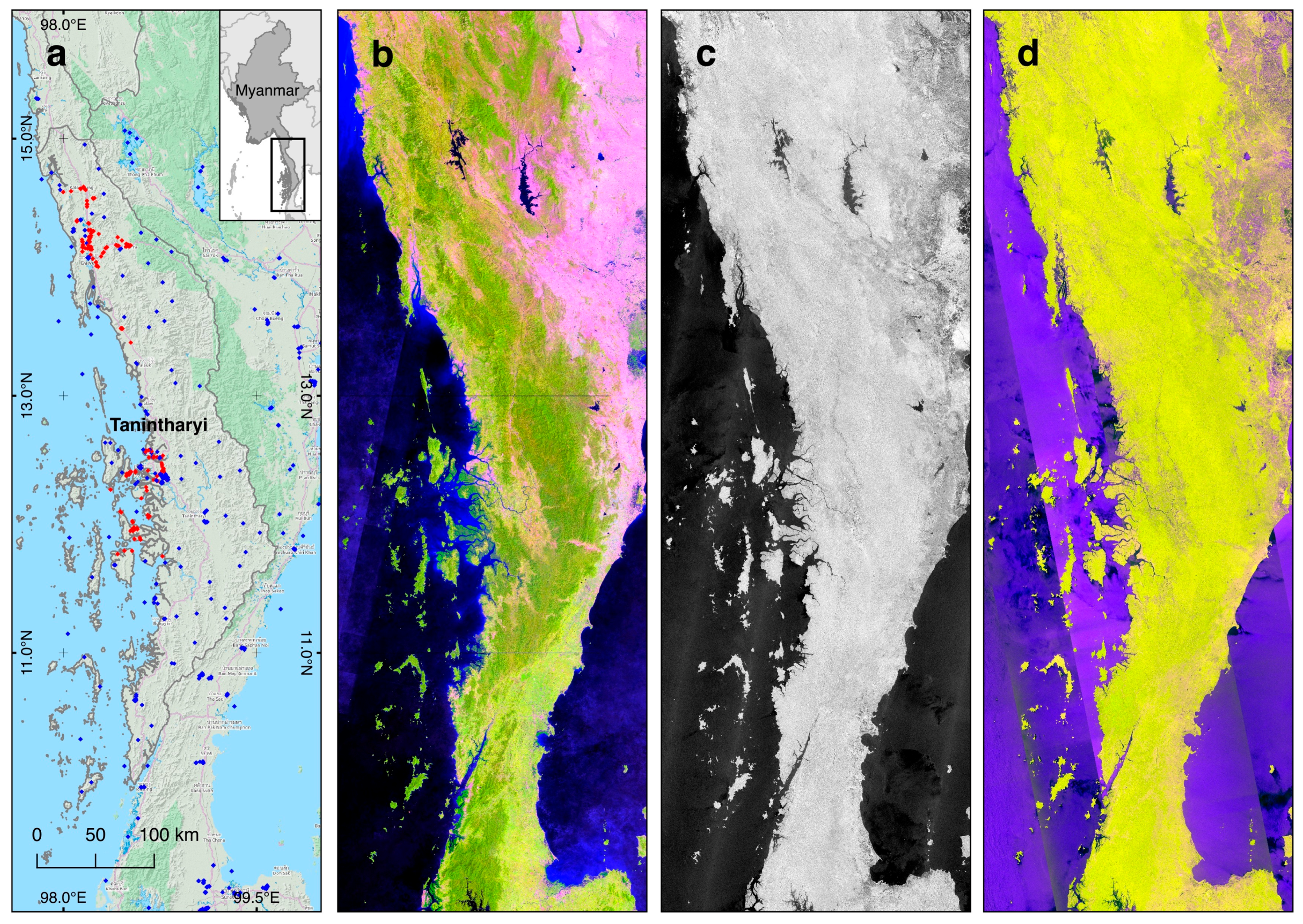
2.1. Study Area

The Tanintharyi Region in southern Myanmar (from ~9° to 16°N and ~97° to 100°E) has a land area of 43,345 km² extending from north to south (Figure 1). The coastal areas border the Andaman Sea to the west and the mountainous Tenasserim Hills (with highest elevation at 2072 m above sea level) are located east along its border with Thailand. The region has a tropical monsoon climate (Am) under the Köppen–Geiger climate classification system [39], and experiences three seasons including summer (February to May), rainy (May to October), and winter (November to February). The mean annual rainfall ranges from 3865 to 5594 mm with average annual temperatures from 26.5 to 26.9 °C across the region [40], which supports tropical evergreen broadleaf forests in most upland (terra firma) zones, mixed deciduous forests in parts of north and northeast Tanintharyi, and mangrove forests in the coastal intertidal zone [41,42].

Despite extensive deforestation experienced in peninsular Thailand and elsewhere, Tanintharyi still holds one of the largest remaining lowland forests in the Indochinese and Sundaic regions of Southeast Asia, having been largely spared due to armed conflict between the Karen ethnic group and the Burmese national government [43]. The forests of Tanintharyi are situated in the biologically rich transition zone of these two biogeographic regions, thereby supporting various globally important threatened species such as tiger (Panthera tigris), Gurney’s pitta (Pitta gurneyi), Sunda pangolin (Manis javanica), Asian elephant (Elephas maximus), and Malayan tapirs (Tapirus indicus) [43,44,45,46,47].

In Myanmar, Tanintharyi is considered an important economic region for the expansion of large-scale agribusiness concessions for crops such as oil palm and rubber, promoted as a dual economic development and poverty alleviation strategy under the government’s 30-year Agricultural Master Plan [48,49]. Of the almost 5400 km² of intact forests converted into various plantations from 2002 to 2014 across Myanmar, Tanintharyi had an expansion of 754.40 km² in plantations—the third highest in the country—accounting for almost 41% of the total intact forest loss within Tanintharyi [50]. Commercial agriculture expansion, particularly from large-scale agro-industrial development, has been identified therefore as a key driver of deforestation that is likely to lead to dramatic future expansion into remaining forests (e.g., [35,38,43,51]).

2.2. Data

2.2.1. Satellite Data

In this study, we used a combination of optical and radar satellite data for land cover change analysis. For optical data, we used the Landsat-5 Thematic Mapper (TM) and the Landsat-8 Operational Land Imager (OLI), specifically the calibrated top-of-atmosphere (TOA) reflectance products available through the Google Earth Engine (available online: https://earthengine.google.com, accessed on 15 September 2016) public data catalog. The Landsat datasets covering our study area were then imported as image collections into Google Earth Engine, a cloud-based geospatial analysis platform [52], for subsequent pre-processing tasks.

For radar data, we used freely available global L-band (long wavelength, ~23 cm) Synthetic Aperture Radar (SAR) mosaic datasets, from the Japan Aerospace Exploration Agency’s (JAXA) Japan Earth Resources Satellite (JERS-1) and the Advanced Land Observing Satellite-2 Phased Array L-band Synthetic Aperture Radar-2 (ALOS-2/PALSAR-2), downloaded from the JAXA ALOS Research and Application Project (available online: http://www.eorc.jaxa.jp/ALOS/en/palsar_fnf/fnf_index.htm, accessed on 16 August 2016). The JERS-1 data were available from 1992-1998 and ALOS-2/PALSAR-2 was available from 2014 onwards [53,54]. Each 1 x 1-degree mosaic tile (4500 × 4500 pixels), provided at 25 m spatial resolution, consists of the following data layers: backscattering coefficients (i.e., horizontal transmit-horizontal receive (HH) polarization for JERS-1 data; HH and horizontal transmit-vertical receive (HV) polarization for ALOS-2/PALSAR-2 data), observation date, local incidence angle, and processing mask information [55]. The SAR backscattering coefficient layers were pre-processed by JAXA using their Sigma-SAR processor, which involved radiometric and geometric calibration, ortho-rectification, slope correction, co-registration, and intensity tuning of neighboring strip data [56]. Twenty-one mosaic tiles were collated to cover Tanintharyi Region at each time point, 1995 and 2015, totaling 42 tiles. We did not observe any problems with the radar datasets (e.g., missing data, stripes) after a visual inspection of the mosaic tiles.

2.2.2. Reference Data and Classification Scheme

We defined land cover classes through a combination of field verification and visual interpretation of high-resolution imagery available from Google Earth Pro (available online: https://www.google.com/earth/desktop/, accessed on 1 October 2016). Ground truth data from field verification were collected in Tanintharyi in 2015 and 2016 by the Smithsonian Institution, Virginia, USA; Fauna & Flora International, Yangon, Myanmar; and EcoDev/ALARM, Yangon, Myanmar. Visual interpretation of reference imagery was based on elements that help to identify land cover features such as location, size, shape, tone/color, shadow, texture, and pattern [57]. We identified land cover classes (

Table 1. Description of the land cover classes of the Tanintharyi Region, Myanmar.

Code	Land Cover Class	Description
FOR	Forest	Forest with tree canopy cover >80%
MNG	Mangrove	Mangrove cover along coastal areas; tree canopy cover >80%
OPM	Oil Palm Mature	Plantation of mature oil palm with coverage >50%
RBM	Rubber Mature	Plantation of mature rubber trees with coverage >50%
SHB	Shrub/Orchard	Degraded woody vegetation; cultivated land such as cashew, betel nut
RPD	Rice Paddy	Paddy fields with planted rice
BUA	Built-Up Area	Developed land such as buildings, roads, human settlements
BSG	Bare Soil/Ground	Areas of exposed soil or ground; with grass or minimal vegetation
WTR	Water Body	Bodies of fresh/saltwater such as oceans, lakes, rivers; flooded areas

) that were delineated as regions of interest (ROI) for training and testing the classification algorithm.

2.3. Overall Workflow and Data Organisation

Our overall workflow consisted of four stages: image pre-processing, image classification, accuracy assessment, and change analysis (Figure 2). Image pre-processing consisted of two parts: for Landsat data, pre-processing tasks involved creating the best-available-pixel image composites and calculating indices; for SAR data, tasks included creating regional mosaics, speckle filtering, converting to normalized radar cross-sections, and calculating texture measures and indices. Image classification involved creating image stacks from the Landsat and SAR layers, delineating regions of interest, and classifying images using a machine learning classifier. Accuracy assessments included calculating standard accuracy metrics, uncertainty estimates, and statistical tests. Finally, change analysis of single-date classifications for 1995 and 2015 included constructing cross-tabulation matrices and a visualization diagram.

We organized our image data stacks into two sets (

Table 2. Organization of datasets, layer composition for each sensor type in each dataset, and total number of layers per data group.

Sensor Type	Set A		Set B
	1995	2015		2015
Landsat	Landsat-5 TM 7 bands 5 indices 1994–1995 composite	Landsat-8 OLI 7 bands 5 indices 2015–2016 composite		Landsat-8 OLI 7 bands 5 indices 2015–2016 composite
L-band SAR	JERS-1 SAR HH polarization 8 GLCM textures 1995 composite	ALOS/PALSAR-2 HH polarization 8 GLCM textures 2015 composite		ALOS/PALSAR-2 HH and HV polarization 16 GLCM textures 6 indices 2015 composite
Total number of layers per data group
Landsat data	12	12		12
SAR data	9	9		24
Landsat + SAR	21	21		36

). Under Set A, two time points (1995 and 2015) were used for analyzing land cover change over the study area across 20 years. Under Set B, only one time point (2015) was used. For each set, three groups of images were put together for evaluation: Landsat-only group, SAR-only group, and Landsat + SAR group. The Landsat-only group consisted of 12 layers with seven image bands and five indices for both sets. For the SAR-only group, Set A consisted of nine layers for each time point with only the HH polarization and eight derivative texture measures, while Set B consisted of both the HH and HV polarizations, thereby increasing the SAR data layers in Set B to 24 consisting of two polarization channels, six indices, and 16 texture measures. For the Landsat + SAR group, a total of 21 and 36 data layers were used in Set A (at both time points) and Set B, respectively. Note that in Set A, since the 1995 JERS-1 SAR data was originally designed with only the HH polarization, we used only the HH polarization of the 2015 PALSAR-2 data to ensure compatibility of both datasets for land cover change analysis. Then in Set B, we used both HH and HV polarizations to evaluate whether the dual-polarized SAR data (with the additional SAR layers generated from the inclusion of the HV polarization such as HV-derived textures and indices) contribute to improving the classification accuracies and discrimination between land cover types compared to Set A 2015, which only included the single-polarized SAR data (HH polarization and HH-derived textures).

2.4. Image Pre-Processing

2.4.1. Pre-Processing of Landsat Images

We generated Landsat image composites for 1995 and 2015 by extracting the best available observations from multiple Landsat images using pixel-based image compositing, implemented through a user-defined rule-based criteria (e.g., sensor preference, dates of acquisition, exclusion of clouds and shadows) to generate the best-available-pixel image composites [58,59,60,61]. To generate the best-available-pixel image composites using Landsat data, we adapted an image compositing script within the Google Earth Engine environment from the contributions of its user community, specifically the modified scripts by Mariano Gonzalez Roglich (Conservation International) and Juan Doblas (Instituto Socioambiental) on the original Temporal Dark Outlier Mask Compositing script developed by Carson Stam and Ian Housman (Red Castle Resources Inc., Salt Lake City, Utah, USA; United States Forest Service—Remote Sensing Applications Center, Salt Lake City, Utah, USA). The image compositing script, including our minor modifications, executed user-defined criteria to select the best-available-pixel in Landsat TOA images and exported the resulting composite images for subsequent use in image classification. Our user-defined inputs included the extent of our study area (Tanintharyi Region), the base year of the image composite (i.e., 1995, 2015), the number of years (n = 2) and Julian date range (0 to 365 days, or from start to end of year) from where the image composite was drawn, the thresholds for excluding or masking clouds (10% or less) and shadows (z-score = −1), and the Landsat sensors used (i.e., Landsat 5 TM for 1995, Landsat 8 OLI for 2015). A median ee.Reducer function was then applied to the collection of images with unmasked pixels to “reduce” the image collection into a single output image representing the median of the images. The output was generated pixel-wise such that at each pixel location in each band of the output image, the pixel value was the median of all unmasked pixels in the image collection at that location [62]. Our scripts, including the links to the original image compositing scripts, are provided in this paper as supplementary material (see Supplementary Material S1 and S2).

From the Landsat image composites of each year, we calculated a set of five indices including the Normalized Difference Vegetation Index (NDVI; Equation (1); [63,64]), the Enhanced Vegetation Index (EVI; Equation (2); [65,66]), the Soil-Adjusted Total Vegetation Index (SATVI; Equation (3); [67,68]), the Normalized Difference Tillage Index (NDTI; Equation (4); [69]), and the Land Surface Water Index (LSWI; also referred to as Normalized Difference Water Index or modified NDVI; Equation (5); [70,71]). These indices are defined as:

$$\mathit{NDVI}=\frac{{\rho }_{NIR}-{\rho }_{RED}}{{\rho }_{NIR}+{\rho }_{RED}}$$

(1)

$$\mathit{EVI}=2.5*\frac{{\rho }_{NIR}-{\rho }_{RED}}{{\rho }_{NIR}+6.0\ast {\rho }_{RED}-7.5\ast {\rho }_{BLUE}+1.0}$$

(2)

$$\mathit{SATVI}=\frac{{\rho }_{SWIR1}-{\rho }_{RED}}{{\rho }_{SWIR1}+{\rho }_{RED}+0.1}\ast \left(1.1-\frac{{\rho }_{SWIR2}}{2.0}\right)$$

(3)

$$\mathit{NDTI}=\frac{{\rho }_{SWIR1}-{\rho }_{SWIR2}}{{\rho }_{SWIR1}+{\rho }_{SWIR2}}$$

(4)

$$\mathit{LSWI}=\frac{{\rho }_{NIR}-{\rho }_{SWIR1}}{{\rho }_{NIR}+{\rho }_{SWIR1}}$$

(5)

where NIR is near infrared band, RED is red band, BLUE is blue band, and SWIR is shortwave infrared band. We used these optical indices owing to their demonstrated capability in forest and land cover mapping. For example, combining NDVI and LSWI was shown to provide better separation of land cover types, including croplands and forests [72]. Another study found that NDTI, SATVI, and LSWI were influential predictors for discriminating between plantations and forests [25]. Lastly, several studies investigating multi-temporal optical data combined with PALSAR data demonstrated the utility of NDVI, EVI, and LSWI for mapping forests and deciduous rubber plantations (e.g., [28,29,30,73]).

2.4.2. Pre-Processing of JERS-1 SAR and ALOS-2/PALSAR-2 Mosaics

The geo-referenced SAR backscattering coefficient tiles were mosaicked together to form regional mosaics for each year. The 1995 JERS-1 mosaic consisted of a single HH-polarized channel and the 2015 PALSAR-2 mosaic consisted of dual-polarized (HH and HV) channels. After mosaicking, a Refined Lee filter was applied to every channel of the regional mosaics to reduce the effects of speckle apparent in raw SAR imagery and to preserve edge information between adjacent land cover types [74]. The digital numbers (DN) of HH and HV images were converted to sigma-naught values (σ⁰; units in decibel, dB) using Equation (6):

$${\sigma }^0=10\cdot {\log }_{10}\left(D{N}^2\right)+CF$$

(6)

where σ⁰ is the radar backscatter per unit area, DN is the digital number, and CF is the calibration factor with a given value of −84.66 dB for the JERS-1 mosaic and −83.0 dB for the PALSAR-2 mosaic [55]. The date and mask tiles corresponding to each regional raster image were also mosaicked to aid in delineating regions of interest for the classification stage. All layers of the regional mosaics (TIFF file format) were then uploaded as image assets in Google Earth Engine. Except for tile mosaicking and file format conversion done in Quantum GIS v.2.18 (available online: http://www.qgis.org/, accessed on 16 August 2016), speckle filtering and conversion to normalized radar cross-section were implemented using the European Space Agency Sentinel Application Platform Toolbox v.4.1 (ESA SNAP; available online: http://step.esa.int/main/toolboxes/snap/, accessed on 16 August 2016).

A set of texture measures and indices were derived from the SAR regional mosaics to provide additional information for land cover classification. The texture measures were calculated for both Sets A and B, while indices were computed only for Set B to make use of both the HH and HV polarization channels. For Set A, the texture measures were calculated from the HH-polarized channel of the 1995 and 2015 mosaics, resulting in eight additional image layers per year. For Set B, the texture measures were calculated separately from the HH and HV polarization channels, resulting in 16 additional image layers for the 2015 mosaic.

We calculated texture measures from SAR data to improve the classification accuracies of broad land cover types [75,76,77,78]. We used second-order texture measures, which consider the spatial relationships between groups of two neighboring pixels to a certain direction within a window. Deriving these texture measures involved the calculation of Grey-Level Co-occurrence Matrices (GLCM), a concept first described by Haralick et al. [79], which outline the distance and angular relationships among a neighborhood of pixels [80]. In this study, we used eight texture measures including contrast (CON), dissimilarity (DIS), and inverse difference moment (IDM), which describe the degree of contrast between pixels; angular second moment (ASM) and entropy (ENT), which describe regularity in the pixels within a neighborhood of pixels; and mean (AVG), correlation (COR), and variance (VAR), which measure the statistics derived from the GLCM [76,80]. The textural attributes were derived from the average of the directional bands within a 3 × 3 neighborhood size using the glcmTexture function in Google Earth Engine (based on Equations (7)–(14); [79,81]):

$$ASM={\displaystyle \sum }_i{\displaystyle \sum }_j{\left\{p\left(i,j\right)\right\}}^2$$

(7)

$$AVG={\displaystyle \sum }_{i=2}^{2N_g}\left(i{p}_{\left(x+y\right)}\left(i\right)\right)$$

(8)

$$CON={\displaystyle \sum }_{n=0}^{N_g-1}{n}^2\left\{{\displaystyle \sum }_{i=1}^{N_g}{\displaystyle \sum }_{j=1}^{N_g}p\left(i,j\right)\right\},\left|i-j\right|=n$$

(9)

$$COR=\frac{{{\displaystyle \sum }}_i{{\displaystyle \sum }}_j\left(i,j\right)p\left(i,j\right)-{\mu }_x{\mu }_y}{{\sigma }_x{\sigma }_y}$$

(10)

$$DIS={\displaystyle \sum }_{n=1}^{N_g-1}n\left\{{\displaystyle \sum }_{i=1}^{N_g}{\displaystyle \sum }_{j=1}^{N_g}p{\left(i,j\right)}^2\right\},\left|i-j\right|=n$$

(11)

$$ENT=-{\displaystyle \sum }_i{\displaystyle \sum }_{j}p\left(i,j\right)\log \left(p\left(i,j\right)\right)$$

(12)

$$IDM={\displaystyle \sum }_i{\displaystyle \sum }_j\left(\frac{1}{1+{\left(i-j\right)}^2}\right)\cdot p\left(i,j\right)$$

(13)

$$VAR={\displaystyle \sum }_i{\displaystyle \sum }_j{\left(i-\mu \right)}^2\cdot p\left(i,j\right)$$

(14)

where p(i,j) is the (i,j) entry in a normalized grey-level spatial dependence matrix; N_g is the number of distinct grey levels in the quantized image; μ_x and μ_y are the means of p_x and p_y; and σ_x and σ_y are the standard deviations of p_x and p_y.

We subsequently derived six additional indices from the raw SAR backscattering coefficient mosaics, including simple ratios of the HH and HV polarization channels (RAT1, RAT2, Equations (15) and (16)), the Average (AVE, Equation (17)), and Difference (DIF, Equation (18)), which in addition to the HH and HV channels were demonstrated to yield good accuracies for discriminating forest, non-forest, and coconut palms [82], and for mapping broad land cover types such as forest, cropland, urban areas, and water [73,83,84,85]. The DIF image provided good separability among plantation species such as oil palm and rubber [86]. We also calculated the Normalized Difference Index (NDI, Equation (19)), which has been applied in detecting new fronts of deforestation [87]; and the NL Index (Equation (20)), which was demonstrated to improve overall accuracies of L-band SAR data for land cover classification [77]. The SAR indices are defined as:

$$RAT1=\frac{HH}{HV}$$

(15)

$$RAT2=\frac{HV}{HH}$$

(16)

$$AVE=\frac{HH+HV}{2}$$

(17)

$$DIF=HH-HV$$

(18)

$$NDI=\frac{HH-HV}{HH+HV}$$

(19)

$$NLI=\frac{HH*HV}{HH+HV}$$

(20)

2.5. Image Classification

2.5.1. Creation of Image Stacks

Both Landsat and L-band SAR data products were generated with high geometric accuracy [56,88]. A good spatial alignment was observed between the two datasets; hence no further processing was done on the final image stacks. The final Landsat-only image stacks for Sets A and B consisted of 12 layers, including seven bands (i.e., BLUE, GREEN, RED, NIR, SWIR1, SWIR2, TIR) and five indices (i.e., NDVI, EVI, SATVI, NDTI, LSWI). The final SAR-only image stacks for Set A 1995 and Set A 2015 consisted of nine layers each (i.e., HH and derived HH textures including ASM, AVG, CON, COR, DIS, ENT, IDM, VAR), and the final SAR-only image stack for Set B 2015 consisted of 24 layers in total (i.e., HH and HV plus their derived textures, RAT1, RAT2, AVE, DIF, NDI, NLI). The final Landsat + SAR image stacks for Set A 1995 and Set A 2015 consisted of 21 layers each, and 36 layers in total comprised the final Landsat + SAR image stack for Set B 2015 (Table 2).

2.5.2. Delineation of Regions of Interest

We separately digitized 1995 and 2015 polygons representing ROIs across the study area within the Google Earth Engine scripting environment. The final set of ROIs consisted of 50 polygons from each land cover class, totaling 450 polygons for nine land cover classes in each year. The 2015 ROI polygons were delineated based on ground truth data, the Landsat and SAR image stacks, and high-resolution imagery available from Google Earth Pro. The polygons were examined by visual interpretation using the time-series high-resolution images in Google Earth Pro and several image composites, including natural color (Landsat-5 Bands 321; Landsat-8 Bands 432), false color (Landsat-5 Bands 432/543; Landsat-8 Bands 543/654; PALSAR-2 HH-HV-HH/HV; SAR RGB HH95-HH95-HH15), and vegetation indices (e.g., NDVI) to check the consistency between polygons and imagery and to develop a robust training/testing dataset.

We implemented a different scheme for delineating 1995 ROI polygons. Due to the absence of ground truth data and high-resolution imagery for 1995, we developed individual mask layers for specific land cover classes to aid in delineating ROIs for classifying the 1995 image stacks. These masks were generated specifically for Oil Palm Mature, Rubber Mature, and Shrub/Orchard classes such that a mask layer would consist of two values: 1 for pixels where ROI polygons can be digitized, and 0 for excluded pixels. To generate the masks, we first extracted the image statistics based from the 2015 Landsat and SAR image stacks using the corresponding 2015 ROIs. From the image statistics, we then constructed box-whisker plots to visualize the distributions of reflectance/backscatter values per land cover type against each optical band/radar channel (predictor variables). Predictor variables deemed capable of discriminating these land cover classes were chosen based on visual assessment of the plots where the classes were separable based on their distributions (see Supplementary Material S3). We subsequently implemented a decision tree classifier to determine thresholds in these chosen optical bands/radar channels from which the masks were calculated. These masks together with the 1995 image stacks were used to delineate ROIs for these classes. The box-whisker plots and decision trees were generated using ggplot2 and tree packages [89,90], respectively, in R Software for Statistical Computing v.3.3.2 ([91]; available online: http://www.R-project.org/, accessed on 15 February 2017). For the remaining land cover classes Forest, Mangrove, Rice Paddy, Built-Up Area, Bare Soil/Ground, and Water Body, we delineated the 1995 ROIs by visually interpreting the 1995 image stacks and contextually examining the 2015 ground truth data and available images. The final polygons were imported as feature collections in Google Earth Engine scripting environment.

2.5.3. Sampling Design

We adopted a simple random sampling design to achieve our accuracy assessment objectives, which involves calculating unbiased accuracy and uncertainty estimates. To calculate the required sample size, we used Equation (21) [92]:

$$n=\frac{z^{2}O\left(1-O\right)}{d^2}$$

(21)

where O is the overall accuracy expressed as a proportion, z is a percentile from the standard normal distribution, and d is the desired half-width of the confidence interval or margin of error. Aiming for an overall accuracy of 0.90, z = 1.96 for a 95% confidence interval, and a 2.5% margin of error, we obtained a total sample size of n = 553.

A 30-m spatial resolution was used as the scale of the ROIs used to classify the Landsat-only and Landsat + SAR image stacks while a 25-m spatial resolution was used as the scale of the ROIs used to classify the SAR-only image stacks. The ROIs were then partitioned into training and testing polygons. Each polygon was assigned a random number between 0 and 1 using the randomColumn and sampleRegions functions in Google Earth Engine, then polygons with assigned values ≤0.70 were segregated as training data and polygons with values >0.70 as testing data. After splitting the ROIs into training and testing polygons, we independently assigned a random number between 0 and 1 to each pixel within each of the training polygons and in each of the testing polygons using the same Google Earth Engine functions. Pixels within training polygons with assigned values ≤0.70 were selected as training pixels, and pixels within testing polygons with assigned values ≤0.70 were selected as testing pixels. We implemented this sampling design to avoid potential bias from having spatially dependent training and testing data [93]. The total number of pixels used for training and testing the Landsat-only, SAR-only, and Landsat + SAR image stacks for each set are presented in

Table 3. Number of pixels used as training and testing pixels for classification. Note that L = Landsat; J = JERS; P = PALSAR; and L + J and L + P indicate combined Landsat and SAR data.

	Set A 1995			Set A 2015; Set B 2015
	L	J	L + J	L	P	L + P
Training	1490	2112	1490	1441	2065	1426
Testing	632	906	632	606	868	606
Total	2122	3018	2122	2047	2933	2032

.

2.5.4. Classification Using Random Forests

We employed Random Forests, an ensemble, non-parametric, machine learning classifier [94], for supervised land cover classification. Random Forests was chosen due to its improved performance in accurately classifying land cover (e.g., [95,96]) and discriminating plantations such as oil palm and rubber (e.g., [25,97]), its computational efficiency and ability to handle high-dimensional, multi-source datasets (e.g., [98,99]), and its robustness against overfitting [94,99]. Random Forests emerged as the best family of classifiers in a study evaluating 179 classifiers from 17 families (e.g., support vector machines, neural networks, discriminant analysis, Bayesian, decision trees, among others) for classifying hundreds of different real world datasets [100]. In this study, the Random Forests classifier in Google Earth Engine was trained using the training data extracted from the sets of image stacks (Table 3) based on the following parameters: 100 decision trees created per class, the square root of the number of variables as the number of variables used for each node split, 10 as the minimum size of a terminal node, and a 0.50 fraction of the input to bag per tree.

We were also interested in variable importance, a feature of Random Forests [94], to determine the important variables used in the classification of the sets of image stacks. To implement the variable importance feature, we first extracted the image statistics based on the sets of image stacks (i.e., Sets A and B; Landsat-only, SAR-only, and Landsat + SAR), and the ROI polygons (i.e., 1995, 2015) corresponding to a specific image stack. Using the image statistics from the training pixels, we then determined the important predictor variables used in the classification of the sets of image stacks using the randomForest package [101] in R software, particularly using the mean decrease in accuracy (permutation importance) as the measure of variable importance.

2.6. Accuracy Assessment

Using the testing data to evaluate the land cover maps from each set, we evaluated the classification results using standard accuracy assessment metrics including error matrix, overall accuracy, and user’s and producer’s accuracies [102], following the good practice recommendations for assessing classification accuracies [103]. For simple random sampling, we used the equations from [104] to calculate the unbiased accuracy estimates and confidence intervals. As recommended, the error matrix should be reported in terms of estimated area proportions and not in terms of sample counts.

To do this, we first calculated for the map marginal proportions, W_i, or the proportion of the map within each map class, by dividing the area of each class by the total area of the classified map. From the error matrix, we then calculated the individual cell probabilities, ${\widehat{p}}_{ij}$, which represents the proportion of area of the entire classified map that has a map class i, a reference class j, and sample counts n_ij using Equation (22):

$${\widehat{p}}_{ij}=W_i\frac{n_{ij}}{n_{i·}}$$

(22)

We subsequently calculated the true marginal proportions, ${\widehat{p}}_{·k}$, the post-stratified estimator for simple random sampling, which represents the proportion of area of class k (of q classes) as determined from the reference classification, and where n_ik is the sample count at cell (i,k) in the error matrix, W_i is the area proportion of map class i using Equation (23):

$${\widehat{p}}_{·k}={\displaystyle \sum }_{i=1}^q{W}_i\frac{n_{ik}}{n_{i·}}$$

(23)

Using these true marginal proportions, we then calculated the unbiased overall, user’s, and producer’s accuracies using the respective formulas of these accuracy metrics. Finally, we calculated the sampling variability associated with the accuracy estimates, particularly of the overall, user’s, and producer’s accuracies using Equations (24)–(26) for the variances, and Equation (27) for the confidence intervals where $V\left(\widehat{O}\right)$, $V\left({\widehat{U}}_i\right)$, and $V\left({\widehat{P}}_j\right)$, are the variance estimators of the unbiased overall ($\widehat{O})$, user’s (${\widehat{U}}_i)$, and producer’s (${\widehat{P}}_j)$ accuracies, respectively:

$$V\left(\widehat{O}\right)={\displaystyle \sum }_{i=1}^q{p}_{ii}\frac{(W_i-p_{ii})}{W_i{n}_{ij}}$$

(24)

$$V\left({\widehat{U}}_i\right)=p_{ii}\frac{(W_i-p_{ii})}{W_i^2{n}_{ij}}$$

(25)

$$V\left({\widehat{P}}_j\right)=p_{ii}{p}_j^{-4}\left[p_{ii}{\displaystyle \sum }_{j\ne 1}^q{p}_{ij}\frac{(W_i-p_{ij})}{W_i{n}_{ij}}+\frac{(W_j-p_{ii}){(p_j-p_{ii})}^2}{W_j{n}_{ij}}\right]$$

(26)

$$\widehat{O}\pm 2{\left[V\left(\widehat{O}\right)\right]}^{\frac{1}{2}}, {\widehat{U}}_i\pm 2{\left[V\left({\widehat{U}}_i\right)\right]}^{\frac{1}{2}}, {\widehat{P}}_j\pm 2{\left[V\left({\widehat{P}}_j\right)\right]}^{1/2}$$

(27)

We calculated the F-score of each land cover class for all image stacks in both sets to determine the degree of discrimination of a given land cover class given a particular image stack (i.e., Landsat-only, SAR-only, Landsat + SAR). The F-score is calculated using Equation (28):

$$f1=\frac{2\ast \left(U{A}_C\ast P{A}_C\right)}{U{A}_C+P{A}_C}$$

(28)

where UA_c and PA_c is the user’s and producer’s accuracy of a particular land cover class [105,106]. To evaluate the statistical significance of the difference between the overall accuracies of classification results, we used the McNemar’s test following Equation (29):

$$z=\frac{f_{12}-f_{21}}{\sqrt{f_{12}+f_{21}}}$$

(29)

where f₁₂ represents the number of samples correctly classified in the first classification, but incorrectly in the second classification, and f₂₁ represents the number of samples correctly classified in the second classification, but incorrectly in the first classification [107]. We assessed the results at α = 0.05 significance level with a z = 1.96 critical value. We computed the standard accuracy assessment metrics and the F-score in Google Earth Engine, the unbiased accuracy and uncertainty estimates in Microsoft Excel, and the McNemar’s tests using the exact2x2 package [108] in R software.

2.7. Change Analysis

Each classified image was post-processed with a 3 × 3 mode filter using the reduceNeighborhood function in Google Earth Engine to smooth isolated pixels. We then used these images for constructing cross-tabulation matrices to summarize the area and percentage of land cover change from 1995 to 2015 using the Land Cover Change function of the Semi-Automatic Classification Plugin in Quantum GIS, which implements map comparison to calculate the difference between a reference and a new classification raster map [109,110]. To complement the cross-tabulation matrices, we plotted the change values in the form of a Sankey diagram using an online generator (available online: https://sankey.csaladen.es/#, accessed on 11 January 2018). Sankey diagrams, traditionally applied in the analysis of flows of energy, materials, and other system processes, have been recently employed in land use/cover change studies for visualizing land cover change transitions [111].

3. Results

3.1. Comparison of Combined versus Individual Sensor Data for Land Cover Classification

For both Sets A and B, the Landsat + SAR data produced the highest unbiased overall accuracies (92.96% to 93.83%), followed by Landsat-only data (91.20% to 91.93%) (

Table 4. Overall accuracies (%) from the classification results for each set and each image group, and results of the McNemar’s tests for (a) Landsat-only vs. Landsat + SAR data for each set, and for (b) Set A vs. Set B data for the 2015 Landsat + SAR data. Results of the McNemar’s tests show the z-scores and p-values (in parentheses).

Image Group	Set A		Set B
	1995	2015	2015
Overall accuracies
Landsat-only	91.20	91.93	91.93
SAR-only	64.78	56.01	71.43
Landsat + SAR	93.83	92.96	93.79
McNemar's tests
(a) Landsat-only vs. Landsat + SAR within each year	2.00 (0.1573)	28.90 (0.00000008)	34.78 (0.000000004)
(b) Landsat + SAR, Set A vs. Set B		3.00 (0.08326)

, z = 2.00 to 34.78; p = 4.0 × 10⁻⁹ to 0.1573). As expected, accuracies from SAR-only data were substantially lower (56.01% to 71.43%); we evaluated SAR-only data for classifying nine land cover classes for completeness although cognizant that the data would achieve low accuracies. The Landsat + SAR data in Set B (with its additional SAR layers) improved accuracy from 92.96% to 93.79%, but the increase in accuracy was not significantly higher than Set A (z = 3.00; p = 0.08326). From this point forward, we focus on the Landsat + SAR data owing to its better overall accuracies compared to individual sensors, although we note that in Set A 1995 the overall accuracies of Landsat + SAR was not significantly higher than Landsat-only data.

A total of 30 table cells (56%) showed improvement in either UA or PA with Landsat + SAR compared to Landsat-only data, whereas only 11 cells (20%) showed that Landsat-only was better than Landsat + SAR data; 13 cells (24%) showed no difference (

Table 5. User’s (UA) and producer’s (PA) accuracies of land cover classes from the classification results of Landsat + SAR data, and the difference of UA and PA between Landsat + SAR vs. Landsat-only data. Numbers in bold indicate an improvement of at least 10% over Landsat-only data, and negative values indicate lower UA and PA for Landsat + SAR compared to Landsat-only data.

Land Cover Type	Set A				Set B
	1995		2015		2015
	UA	PA	UA	PA	UA	PA
Landsat + SAR
Forest	0.9898	0.9661	0.9909	0.9375	0.9928	0.9000
Mangrove	0.6616	1.0000	1.0000	1.0000	1.0000	1.0000
Oil Palm Mature	1.0000	0.9136	0.7012	0.8393	0.6851	0.8545
Rubber Mature	1.0000	1.0000	0.6600	0.9184	0.6796	0.9375
Shrub/Orchard	0.9722	0.7778	0.8282	0.7143	0.8618	0.7714
Rice Paddy	0.6905	0.7465	0.9731	0.8553	0.9334	0.9041
Built-Up Area	0.8603	0.9348	1.0000	1.0000	1.0000	1.0000
Bare Soil/Ground	0.6963	0.9239	0.8765	0.9518	0.9453	0.9625
Water Body	1.0000	1.0000	1.0000	1.0000	1.0000	1.0000
Difference (Landsat + SAR - Landsat-only)
Forest	0.0006	0.0317	–0.0091	–0.0208	–0.0072	–0.0583
Mangrove	0.0682	0	0.0597	0	0.0597	0
Oil Palm Mature	0	0	0.0460	0.0029	0.0299	0.0182
Rubber Mature	0	0	–0.0131	0.0093	0.0065	0.0284
Shrub/Orchard	–0.0157	0.1256	0.0689	0.0621	0.1025	0.1193
Rice Paddy	0.0646	–0.0414	–0.0232	0.0504	–0.0629	0.0992
Built-Up Area	0.2987	0.0098	0.0995	0.4921	0.0995	0.4921
Bare Soil/Ground	0.1098	0.0552	0.1719	–0.0112	0.2407	–0.0005
Water Body	0	0	0	0	0	0

). The Landsat + SAR data produced at least 10% improvement over Landsat-only data in either UA or PA of Built-Up Area, Bare Soil/Ground, and Shrub/Orchard. However, for land cover classes in which UA or PA did not improve at least 10% (e.g., Forest, Mangrove, Oil Palm Mature, Rubber Mature, Rice Paddy), accuracies were generally high (>80%). Lower UA or PA with Landsat + SAR data was observed for Mangrove (UA = 66.16%), Oil Palm Mature (UA = 68.51%), Rubber Mature (UA = 66% to 67.96%), Shrub/Orchard (PA = 71.43% to 77.78%), and Rice Paddy (UA = 69.05%). The unbiased UA and PA estimates and the error matrices expressed in terms of estimated area proportions of all classification results are reported in this paper as supplementary material (Supplementary Materials S4 and S5).

Although SAR-only data were ineffective in classification, the SAR layers contributed to the most important predictor variables in Landsat + SAR data (

Table 6. Ten most important predictor variables from the classification results of Landsat-only (L), SAR-only (J or P), and Landsat + SAR (L + J or L + P) data. Numbers in parentheses below each variable indicate variable importance scores based on mean decrease in accuracy (permutation importance).

Set A						Set B
1995			2015			2015
L	J	L + J	L	P	L + P	L	P	L + P
SATVI (17.09)	HH AVG (38.63)	HH AVG (18.05)	SATVI (15.75)	HH AVG (40.31)	SATVI (13.85)	SATVI (16.18)	HV (21.01)	SWIR1 (12.93)
NIR (16.77)	HH (22.57)	NIR (13.18)	TIR (15.28)	HH (21.28)	GREEN (13.82)	TIR (13.81)	HH AVG (15.47)	GREEN (10.79)
TIR (15.79)	HH VAR (15.25)	EVI (12.42)	EVI (13.39)	HH VAR (19.28)	HH AVG (12.53)	NDVI (13.79)	HV AVG (14.59)	TIR (10.57)
EVI (14.98)	HH DIS (13.83)	SATVI (12.41)	NDVI (13.20)	HH DIS (15.62)	SWIR1 (11.71)	EVI (13.73)	HH VAR (13.39)	SATVI (10.05)
SWIR1 (14.88)	HH IDM (13.58)	SWIR1 (11.46)	RED (12.30)	HH CON (15.31)	EVI (11.28)	GREEN (12.89)	NLI (13.28)	SWIR2 (9.74)
NDVI (14.28)	HH CON (13.33)	HH (11.17)	SWIR1 (11.96)	HH IDM (11.85)	NDVI (10.63)	NIR (12.01)	AVE (12.84)	NDVI (9.63)
SWIR2 (11.81)	HH COR (6.48)	HH CON (10.97)	LSWI (11.85)	HH COR (6.71)	TIR (10.59)	SWIR1 (11.39)	NDI (12.75)	HV AVG (9.07)
BLUE (11.67)	HH ENT (1.87)	NDVI (10.59)	NDTI (10.78)	HH ENT (0.04)	SWIR2 (10.39)	SWIR2 (11.03)	HH (12.54)	EVI (9.04)
LSWI (11.22)	HH ASM (0.52)	LSWI (10.00)	SWIR2 (10.42)	HH ASM (0.00)	LSWI (10.08)	NDTI (10.42)	DIF (11.68)	NDTI (8.41)
GREEN (10.70)		SWIR2 (9.89)	NIR (9.79)		NIR (9.77)	LSWI (10.19)	HH VAR (11.63)	NIR (8.38)

). All optical indices were important variables for Landsat-only data. For Landsat + SAR data, HH AVG, SATVI, NIR, EVI, SWIR1, NDVI, LSWI, and SWIR2 were consistently the most important variables in Set A. In Set B, among 36 layers, the most important variables included HV AVG sum average (mean) texture for the SAR layers; and SWIR1 and SWIR2, four optical indices (SATVI, NDVI, EVI, and NDTI), GREEN, TIR, and NIR for optical layers. For Landsat-only data, SATVI, TIR, NIR, EVI, NDVI, SWIR1, SWIR2, and LSWI were consistently the most important variables in both Sets A and B.

F-scores from both Landsat + SAR and Landsat-only data showed comparatively good discriminative capabilities for classifying Forest and Mangrove (>0.80), except for Mangrove in Set A 1995 (

Table 7. F-scores of land cover classes from the classification results of the Landsat-only (L), SAR-only (J or P), and Landsat + SAR (L + J or L + P) data.

Land Cover Class	Set A						Set B
	1995			2015			2015
	L	J	L + J	L	P	L + P	L	P	L + P
Forest	0.9610	0.4690	0.9778	0.9787	0.2733	0.9635	0.9787	0.6527	0.9441
Mangrove	0.7448	0.0120	0.7963	0.9692	0.5937	1.0000	0.9692	0.6247	1.0000
Oil Palm Mature	0.9548	0.3081	0.9548	0.7348	0.4536	0.7641	0.7348	0.5781	0.7605
Rubber Mature	1.0000	0.1888	1.0000	0.7735	0.6226	0.7681	0.7735	0.6833	0.7880
Shrub/Orchard	0.7857	0.0254	0.8642	0.7017	0.2485	0.7670	0.7017	-	0.8141
Rice Paddy	0.6976	0.4191	0.7174	0.8904	0.2597	0.9104	0.8904	0.2097	0.9185
Built-Up Area	0.6989	0.8182	0.8960	0.6495	0.7706	1.0000	0.6495	0.7975	1.0000
Bare Soil/Ground	0.7002	0.2784	0.7941	0.8137	0.3033	0.9126	0.8137	0.5328	0.9538
Water Body	1.0000	0.9553	1.0000	1.0000	0.8278	1.0000	1.0000	0.9219	1.0000

). For Oil Palm Mature and Rubber Mature, discriminative capabilities of Landsat+ SAR and Landsat-only data were high for Set A 1995 (>0.95), but lower in Set A 2015 and Set B 2015 (between 0.73 to 0.79). For most land cover classes, the difference in F-scores between Landsat + SAR and Landsat-only data were less than 0.05, except Shrub/Orchard (by 0.06 to 0.11), Built-Up Area (by 0.19 to 0.35), and Bare Soil/Ground (by 0.09 to 0.14) where Landsat + SAR data had higher F-scores than Landsat-only data.

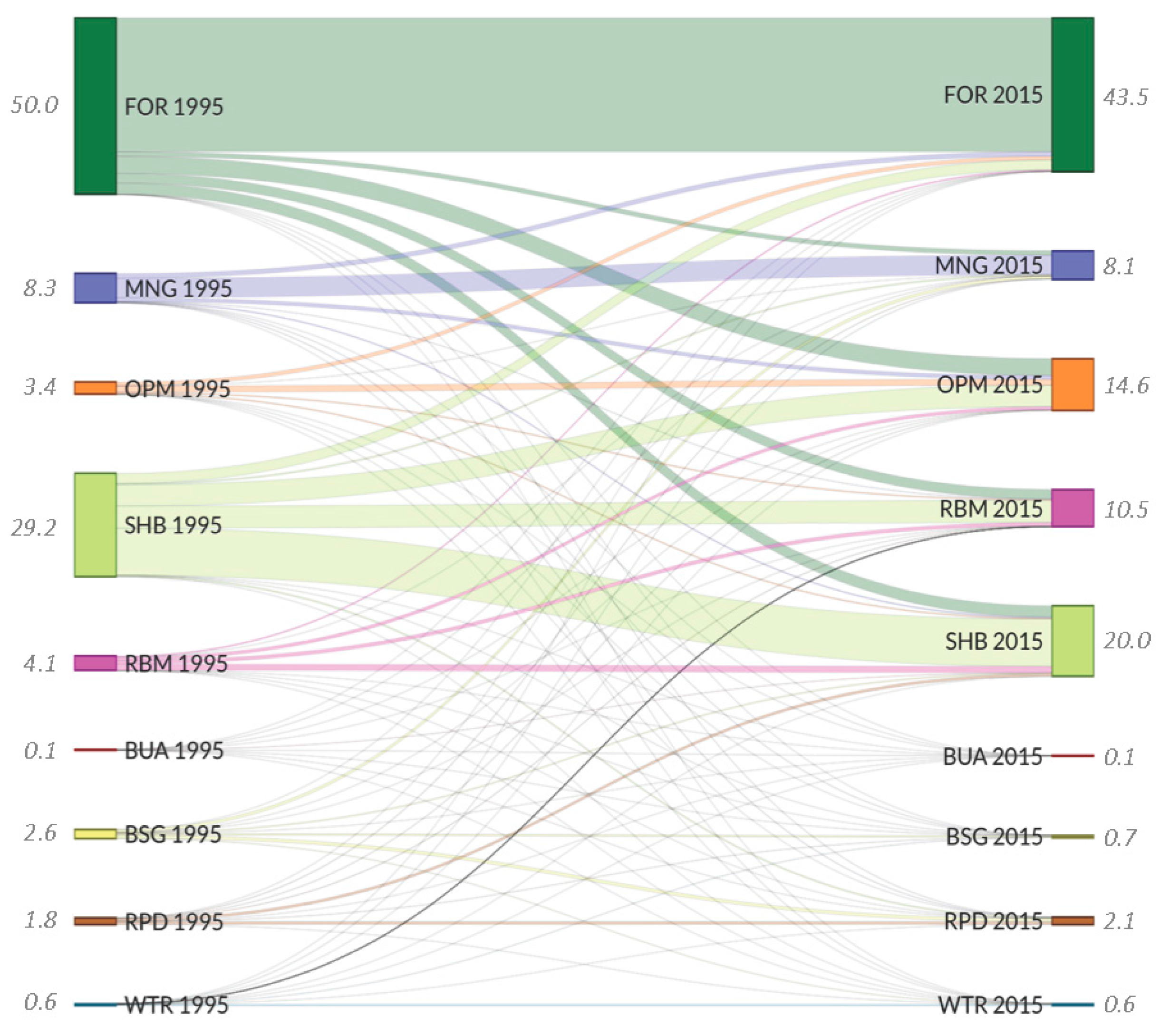
3.2. Land Cover Change in Tanintharyi Region, 1995–2015

Land cover change in the Tanintharyi Region from 1995–2015 was extensive (Figure 3). A total of 16,490 km² (39% of the total landscape) experienced change from 1995–2015. Land cover maps from the Landsat + SAR data further demonstrated the spatially-explicit nature of land cover change dynamics (Figure 3). The major landscape changes included the expansion of rubber and oil palm plantations in the north and south, respectively; and deforestation and forest fragmentation in the south.

For Forest, 76% remained unchanged (16,112/21,245 km²); likewise 67% of Mangrove remained unchanged. Large area changes were observed in Forest, Oil Palm Mature, Rubber Mature, and Shrub/Orchard from 1995 to 2015 (

Table 8. Land cover change matrix from 1995 (rows) to 2015 (columns) based on Landsat + SAR data showing land area (km²) and percentage of total area (%) of land cover classes in Tanintharyi Region, Myanmar.

	2015
1995	FOR	MNG	OPM	RBM	SHB	RPD	BUA	BSG	WTR	Total
Land area (km2)
FOR	16,112	538	2044	1170	1361	15	2	3	0	21,245
MNG	535	2345	432	20	114	34	3	24	5	3511
OPM	441	3	738	124	128	2	0	1	0	1436
RBM	156	1	381	431	751	5	0	0	0	1726
SHB	1210	138	2564	2653	5683	137	4	20	3	12,413
RPD	4	48	24	44	312	337	2	17	0	782
BUA	1	11	3	1	24	6	6	3	0	55
BSG	16	323	21	13	107	364	11	183	51	1089
WTR	4	30	1	0	1	1	1	29	188	255
Total	18,479	3428	6209	4547	8482	901	29	280	247	42,512
Percentage (%)
	FOR	MNG	OPM	RBM	SHB	RPD	BUA	BSG	WTR	Total
FOR	37.90	1.26	4.81	2.75	3.20	0.04	0.00	0.01	0.00	49.97
MNG	1.26	5.52	1.02	0.05	0.27	0.08	0.01	0.06	0.01	8.26
OPM	1.04	0.01	1.74	0.29	0.30	0.00	0.00	0.00	0.00	3.38
RBM	0.37	0.00	0.90	1.01	1.77	0.01	0.00	0.00	0.00	4.06
SHB	2.85	0.33	6.03	6.24	13.37	0.32	0.01	0.05	0.01	29.20
RPD	0.01	0.10	0.06	0.10	0.73	0.79	0.01	0.04	0.00	1.84
BUA	0.00	0.03	0.01	0.00	0.06	0.01	0.01	0.01	0.00	0.13
BSG	0.04	0.76	0.05	0.03	0.25	0.86	0.03	0.43	0.12	2.56
WTR	0.01	0.07	0.00	0.00	0.00	0.00	0.00	0.07	0.44	0.60
Total	43.47	8.06	14.61	10.48	19.95	2.12	0.07	0.66	0.58	100.00

). Forest decreased from 21,245 km² to 18,479 km² (49.97% to 43.47% of total area). Plantations expanded within this 20-year period with Oil Palm Mature increasing from 1436 km² to 6209 km² (3.38% to 14.61% of total area) and Rubber Mature increasing from 1726 km² to 4457 km² (4.06% to 10.48% of total land area). Shrub/Orchard decreased from 12,413 km² to 8482 km² (29.20% to 19.95% of total area). To a lesser extent, changes in Bare Soil/Ground decreased from 1089 to 280 (2.56% to 0.66% of total area); Mangrove decreased from 3511 km² to 3428 km² (8.26% to 8.06% of total area); and Rice Paddy increased from 782 km² to 901 km² (1.84% to 2.12% of total area).

The gross losses/gains between land cover classes showed that transitions between land cover classes were dynamic (Table 8; Figure 4). Focusing on forest conversion and plantation expansion, Forest showed a total net loss of 2766 km² while Oil Palm Mature and Rubber Mature showed a total net gain of 4773 km² and 2731 km², respectively, within the 20-year study period. However, the total gross loss of Forest in 1995 was 5133 km² (i.e., 86% above the total net loss) through conversion to Oil Palm Mature (2044 km²); Shrub/Orchard (1361 km²), Rubber Mature (1170 km²), and; the total gross gain of Forest in 2015 was 2367 km², attributed to the conversion of Shrub/Orchard (1210 km²), Mangrove (535 km²), and Oil Palm Mature (441 km²). The total gross gain of Oil Palm Mature in 2015 was 5471 km², attributed to the conversion of Shrub/Orchard (2564 km²), Forest (2044 km²), and Mangrove (432 km²) into oil palm plantations. The total gross gain of Rubber Mature in 2015 was 4025 km², attributed to the conversion of Shrub/Orchard (2653 km²), Forest (1170 km²), and Oil Palm Mature (124 km²) into rubber plantations.

Shrub/Orchard largely contributed to the changes in forest and plantation expansion (Table 8; Figure 4). Shrub/Orchard showed total net loss of 3931 km² within the same period, and its total gross loss was 6730 km², which were largely conversion into Rubber Mature (2653 km²), Oil Palm Mature (2564 km²), and Forest (1210 km²), and its total gross gain was 2799 km², mainly from the conversion of Forest (1361 km²), Rubber Mature (751 km²), and Rice Paddy (312 km²).

4. Discussion

4.1. Twenty-Year Land and Forest Cover Change in Tanintharyi Region

The Tanintharyi Region is a dynamic landscape, that recently experienced rapid and extensive land use and land cover change over a 20-year period. Despite retaining one of the largest contiguous areas of intact forests in Myanmar [50], Tanintharyi’s biodiverse lowland forests and mangroves have limited geographic extents and are more heavily degraded than upland evergreen forests that are widely distributed in the mountains along the Thailand border [42]. Our results corroborated previous remote sensing-based studies on Tanintharyi that found oil palm and/or rubber plantation expansion leading to widespread forest loss, particularly of lowland forests [43,50,112,113]. Compared to official statistics, our estimate of the total area of oil palm and rubber plantations (10,666 km²) in 2015 was more than four times the reported total area of planted oil palm and rubber (2662 km²) in Tanintharyi in 2012/2013 ([51] citing Ministry of Agriculture and Irrigation). However, a direct comparison is not feasible due to differences in data sources and the lack of transparent and robust government data.

Our results further align with research in other tropical landscapes where commercial tree-based plantations have led to forest conversion, such as Peninsular Malaysia [114], Indonesia [114,115,116], Latin America [117], and Africa [9,118] for oil palm; and China [119,120,121,122] and Cambodia [123] for rubber. The expansion of these plantations in many tropical landscapes has been made possible due to the global demand for agricultural commodities, foreign direct investment, supportive government policies and programs, and the need to secure socio-economic benefits for local communities (e.g., [119,124,125,126,127]).

Landscape change due to agricultural expansion of rice, agricultural boom crops such as oil palm and rubber, and timber/wood extraction and infrastructure development has been widely acknowledged to drive deforestation in Myanmar [35,37,51]. The expansion of agricultural plantations is likely a direct outcome of the Myanmar national government’s policy reforms that liberalized markets and encouraged private sector investments in agriculture [35,48]. Weak land tenure and armed conflict in disputed territories, in addition to formal concessions and economic investment, present a complex interplay of underlying factors that further situates the role of agribusiness concessions in deforestation in Myanmar [35]. It is projected that large-scale, agro-industrial development could potentially lead to widespread future deforestation due to the combined effects of land suitability for crops in remaining large tracts of forests, economic liberalization, unclear land classification, governance challenges, and legal system dysfunctions [36,37,38]. And as observed elsewhere, agricultural plantation expansion in Myanmar could similarly result in negative environmental impacts (e.g., [5,8,12,128,129,130]). Our analysis can be useful to policymakers and planners for evaluating the impacts of the Myanmar government’s agricultural modernization policy.

4.2. Comparison of Combined Landsat and SAR Sensors versus Individual Sensors

Although our results align with previous research on plantations-deforestation in Tanintharyi, our technical approach differed mainly in two ways that improve land cover detection and change observations compared to previous studies in Myanmar. First, we implemented pixel-based image compositing of Landsat imageries for our analysis; thereby creating seamless, cloud-free image composites using the best-available pixel observations [58,59,60,61]. Second, we combined Landsat and L-band SAR data, thereby maximizing the unique range of information detected by these sensors across the electromagnetic spectrum for discriminating various land cover types. Moreover, our results highlighted the dynamic landscape changes occurring in the Tanintharyi Region, such as the degradation and regrowth of forests, the conversion and expansion of oil palm and rubber plantations, and transitions to and from shrub/orchards.

Our study demonstrated that combining Landsat and L-band SAR data outperformed data solely from either sensor alone for land cover classification and change analysis, as shown by improvements in overall accuracies and better user’s and producer’s accuracies for most land cover types. Previous studies investigating sensor synergies of Landsat and L-band SAR at the data level for land cover mapping in tropical areas such as in West Africa [23], and Kalimantan and Riau in Indonesia [22,24] produced similar results yielding the best overall classification accuracies for combined optical and radar sensors over individual sensors. These studies, however, evaluated the combination of Landsat and L-band SAR data for land cover classification at smaller scales (<900 km² for Indonesia; <8000 km² for West Africa) compared to the much larger landscape-scale investigation that we have done. Further, our study evaluated which land cover types the combined optical and radar dataset was most effective, in particular towards the discrimination of tree-based plantations (i.e., oil palm and rubber) and other non-vegetated cover types (i.e., built-up area, bare soil/ground).

We note that our results corroborated the study by Torbick et al. [25], which investigated the fusion of multiple new sensors (i.e., Landsat-8, PALSAR-2, and Sentinel-1A) for mapping tree-based plantation extent in Tanintharyi and West Kalimantan, that showed multi-sensor combination was useful for distinguishing plantations from other land cover types. However, our study did not include C-band SAR data since there was insufficient spatial coverage of historical C-band SAR imagery in 1995 over our study area, and we focused on utilizing combined Landsat and L-band SAR data for identifying patterns of land cover change, specifically estimating forest conversion and plantation expansion, and on comparing classification accuracies based on individual versus combined optical and SAR sensor data.

L-band SAR data proved to be useful owing to its contribution to the most important predictor variables. In our study, texture measures from both co- and cross-polarized channels such as the sum average (mean) and contrast were consistently among the top predictor variables contributing to overall performance of the combined Landsat and SAR data. The HH-polarized backscatter is known to be correlated to the large crown canopies of oil palm although not to trunk height, while for rubber the HH-polarized backscatter is correlated to trunk, branches, and twigs; hence allowing the discrimination between mature oil palm and rubber plantations owing to the difference in scattering mechanisms involved [131]. In our study, the influence of other SAR layers may have been less prominent for identifying oil palm and rubber due to the presence of the additional optical layers, but then had compensated elsewhere in classifying other land cover classes such as built-up areas and bare soil/ground where optical layers had been less effective.

Adding SAR texture attributes contributed to improved classification accuracies of combined optical and SAR datasets, which was similarly observed by Vaglio Laurin et al. [23], albeit less effective and with minimal improvement compared to when added to SAR-only data where the margins of improvement were more significant. Except for the sum average and contrast textures, our study found that other texture attributes were less influential for land cover classification of combined sensor data, which contrasted with other studies that found homogeneity and entropy textures as relevant for improving classification accuracies and for discriminating various land cover classes [22,76]. This difference is likely due to the larger kernel sizes (5 × 5 and above) applied to calculate textures in other studies, which compared to our case was a small kernel size (3 × 3) owing to the computational limitations we experienced in calculating textures of larger neighborhood sizes at landscape scales. Although we opted to use a smaller kernel for this study, we suggest that future work explore the impact of larger kernels for classifying land cover at landscape scales, should computational resources be available.

Some studies conducted in South America (e.g., Ecuador, Peru) have found that Landsat had limited ability to distinguish oil palm from other land cover, which was due to dense palm canopies that rendered optical reflectance bands insensitive to structural geometric characteristics and to spectral differences with other land cover types (e.g., secondary vegetation) [132,133]. In contrast, our results showed that Landsat-only data had good discriminative capability of oil palm (F-scores > 0.95 for 1995 and >0.73 for 2015), which may be due to the combined influence of optical indices and shortwave and thermal infrared bands, which all came to the fore of predictor variables used for identifying most land cover classes. Our findings also corroborated Connette et al. [42], which showed good classification accuracies for mapping oil palm plantations using Landsat, specifically in Tanintharyi Region.

Discriminating nine land cover types in our study area was challenging for L-band SAR-only data [23,134]. Our results therefore clearly suggest that the way to maximize the utility of L-band SAR sensors, at least of single- or dual-polarized SAR products, for detailed mapping and monitoring of land cover in tropical landscapes is through an integrated classification approach of optical and radar data, such as what we have done here. Combining optical and radar data is beneficial to maximize their complementarity, in particular Landsat’s and L-band SAR’s sensitivities to the spectral and geometric/structural characteristics, respectively, of various land cover features [23].

4.3. Potential Applications and Future Work

Government planners and policymakers can use the findings and maps presented in this study to evaluate the impact of the government’s 30-year Agricultural Master Plan initiated in 2000, in particular the expansion of plantations. Our study can potentially be used for further analysis of land cover dynamics to assess the efficiency of the protected areas network in safeguarding important biodiversity and their habitats in the Tanintharyi Region, and testing the potential for mapping plantations of other species (such as teak, eucalyptus, banana, cassava) that are grown in Myanmar and elsewhere. Our results on land use/cover change transitions become essential towards developing some of the future work we envision that will explore understanding spatial determinants and landscape patterns of land use/cover change, simulating spatially explicit future land use/cover change, and assessing historic and future projected wildlife habitat given different development scenarios, of which the results can inform government planning and policy formation.

Leveraging optical Landsat data with full-polarimetric (HH, HV, VH, VV) L-band SAR data, or with multi-frequency (e.g., X-, C-, L-, and P-bands) SAR datasets, can be promising next steps as Earth observation data become more widely accessible, relevant, and integrated in many applications. An emerging opportunity for land change science studies is the growing utility of cloud computing geospatial analysis platforms, combined with the ever-increasing availability of Earth observation data products, which are expected to facilitate multi-scale investigations of land system changes. Exploiting valuable information also becomes challenging as large-scale remote sensing datasets become more available. Hence, incipient developments in deep machine learning approaches such as convolutional neural networks (e.g., [135,136,137,138]) are gaining attention due to their promising capability for automatically extracting valuable contextual information from remote sensing data such as for large-scale land cover classification. Finally, our study can be applied in similar geographic contexts that can help to better understand the associated drivers of ongoing expansion of agricultural plantations and the dynamics of land use/cover change across tropical forest landscapes globally, making our contribution relevant in this growing era of Big Data.

5. Conclusions

Commercial agriculture is considered the leading driver of tropical deforestation globally. In Myanmar, the expansion of agro-industrial plantation development is expected, which can have profound effects on the environment and to local communities. In our study, we set out to evaluate the capability of Landsat and L-band SAR data to estimate forest and land cover conversion cover in Tanintharyi Region over two decades. We found that the combination of Landsat and L-band SAR data was better than individual sensor data through robust and reliable accuracy metrics. Optical indices and texture measures derived from SAR data were prominent predictors for various land cover types within the region, and discriminated tree-based agricultural plantations (oil palm, rubber) from forest and other land cover types. Moreover, we showed that using synergistic optical and radar data provided reliable information on land cover change, particularly forest conversion, plantation expansion, and transitions among various land cover in Tanintharyi Region over two decades. This spatially explicit approach for analyzing landscape changes, when interpreted together with an in-depth understanding of the complex proximate and underlying factors driving these changes, can be used to inform evidence-based spatial planning, policy interventions, and decision-making. Using multiple Earth observation sensors proved useful in generating land cover change information that help to understand dynamic landscape changes in the tropics, and potentially can also support the assessments of the impacts of land use policies and the development of viable solutions for sustainably managing land resources.

References

1. Vitousek, P.M.; Mooney, H.A.; Lubchenco, J.; Melillo, J.M. Human domination of Earth’s ecosystems. Science 1997, 277, 494–499. [Google Scholar] [CrossRef]
2. Foley, J.A.; DeFries, R.; Asner, G.P.; Barford, C.; Bonan, G.; Carpenter, S.R.; Chapin, F.S.; Coe, M.T.; Daily, G.C.; Gibbs, H.K.; et al. Global consequences of land use. Science 2005, 309, 570–574. [Google Scholar] [CrossRef] [PubMed]
3. Foley, J.A.; Ramankutty, N.; Brauman, K.A.; Cassidy, E.S.; Gerber, J.S.; Johnston, M.; Mueller, N.D.; O’Connell, C.; Ray, D.K.; West, P.C.; et al. Solutions for a cultivated planet. Nature 2011, 478, 337–342. [Google Scholar] [CrossRef] [PubMed]
4. Ramankutty, N.; Evan, A.T.; Monfreda, C.; Foley, J.A. Farming the planet: 1. Geographic distribution of global agricultural lands in the year 2000. Glob. Biogeochem. Cycles 2008, 22, GB1003. [Google Scholar] [CrossRef]
5. Ziegler, A.D.; Fox, J.M.; Xu, J. The rubber juggernaut. Science 2009, 324, 1024–1025. [Google Scholar] [CrossRef] [PubMed]
6. Wicke, B.; Sikkema, R.; Dornburg, V.; Faaij, A. Exploring land use changes and the role of palm oil production in Indonesia and Malaysia. Land Use Policy 2011, 28, 193–206. [Google Scholar] [CrossRef]
7. Li, Z.; Fox, J.M. Mapping rubber tree growth in mainland Southeast Asia using time-series MODIS 250 m NDVI and statistical data. Appl. Geogr. 2012, 32, 420–432. [Google Scholar] [CrossRef]
8. Ahrends, A.; Hollingsworth, P.M.; Ziegler, A.D.; Fox, J.M.; Chen, H.; Su, Y.; Xu, J. Current trends of rubber plantation expansion may threaten biodiversity and livelihoods. Glob. Environ. Chang. 2015, 34, 48–58. [Google Scholar] [CrossRef]
9. Vijay, V.; Pimm, S.L.; Jenkins, C.N.; Smith, S.J. The impacts of oil palm on recent deforestation and biodiversity loss. PLoS ONE 2016, 11, e0159668. [Google Scholar] [CrossRef] [PubMed]
10. FAO FAOSTAT. Available online: http://www.fao.org/faostat/en/#data/QC (accessed on 2 August 2017).
11. Tilman, D.; Balzer, C.; Hill, J.; Befort, B.L. Global food demand and the sustainable intensification of agriculture. Proc. Natl. Acad. Sci. USA 2011, 108, 20260–20264. [Google Scholar] [CrossRef] [PubMed]
12. Phalan, B.; Bertzky, M.; Butchart, S.H.M.; Donald, P.F.; Scharlemann, J.P.W.; Stattersfield, A.J.; Balmford, A. Crop expansion and conservation priorities in tropical countries. PLoS ONE 2013, 8, e51759. [Google Scholar] [CrossRef] [PubMed]
13. Lambin, E.F.; Geist, H.J.; Lepers, E. Dynamics of land-use and land-cover change in tropical regions. Annu. Rev. Environ. Resour. 2003, 28, 205–241. [Google Scholar] [CrossRef]
14. DeFries, R.S.; Foley, J.A.; Asner, G.P. Land-use choices: Balancing human needs and ecosystem function. Front. Ecol. Environ. 2004, 2, 249–257. [Google Scholar] [CrossRef]
15. Moran, E.F.; Skole, D.L.; Turner, B.L. The Development of the International Land Use and Land Cover Change (LUCC) Research Program and Its Links to NASA’s Land Cover and Land Use Change (LCLUC) Initiative. In Land Change Science: Observing, Monitoring and Understanding Trajectories of Change on the Earth’s Surface, 2004 ed.; Gutman, G., Janetos, A.C., Justice, C.O., Moran, E.F., Mustard, J.F., Rindfuss, R.R., Skole, D., Turner, B.L., Cochrane, M.A., Eds.; Springer: Dordrecht, The Netherlands; New York, NY, USA, 2012. [Google Scholar]
16. Turner, B.L.; Lambin, E.F.; Reenberg, A. The emergence of land change science for global environmental change and sustainability. Proc. Natl. Acad. Sci. USA 2007, 104, 20666–20671. [Google Scholar] [CrossRef] [PubMed]
17. Rose, R.A.; Byler, D.; Eastman, J.R.; Fleishman, E.; Geller, G.; Goetz, S.; Guild, L.; Hamilton, H.; Hansen, M.; Headley, R.; et al. Ten ways remote sensing can contribute to conservation. Conserv. Biol. 2015, 29, 350–359. [Google Scholar] [CrossRef] [PubMed]
18. Turner, W.; Rondinini, C.; Pettorelli, N.; Mora, B.; Leidner, A.K.; Szantoi, Z.; Buchanan, G.; Dech, S.; Dwyer, J.; Herold, M.; et al. Free and open-access satellite data are key to biodiversity conservation. Biol. Conserv. 2015, 182, 173–176. [Google Scholar] [CrossRef]
19. Giri, C. Remote Sensing of Land Use and Land Cover: Principles and Applications; Remote Sensing Applications Series; CRC Press: Hoboken, NJ, USA, 2012; Volume 20120991. [Google Scholar]
20. Lehmann, E.A.; Caccetta, P.; Lowell, K.; Mitchell, A.; Zhou, Z.-S.; Held, A.; Milne, T.; Tapley, I. SAR and optical remote sensing: Assessment of complementarity and interoperability in the context of a large-scale operational forest monitoring system. Remote Sens. Environ. 2015, 156, 335–348. [Google Scholar] [CrossRef]
21. Reiche, J.; Lucas, R.; Mitchell, A.L.; Verbesselt, J.; Hoekman, D.H.; Haarpaintner, J.; Kellndorfer, J.M.; Rosenqvist, A.; Lehmann, E.A.; Woodcock, C.E.; et al. Combining satellite data for better tropical forest monitoring. Nat. Clim. Chang. 2016, 6, 120–122. [Google Scholar] [CrossRef]
22. Wijaya, A.; Gloaguen, R. Fusion of ALOS PALSAR and Landsat ETM data for land cover classification and biomass modeling using non-linear methods. In Proceedings of the 2009 International Geoscience and Remote Sensing Symposium (IGARSS), Cape Town, South Africa, 12–17 July 2009; Volume 3, pp. 581–584. [Google Scholar]
23. Vaglio Laurin, G.; Liesenberg, V.; Chen, Q.; Guerriero, L.; Del Frate, F.; Bartolini, A.; Coomes, D.; Wilebore, B.; Lindsell, J.; Valentini, R. Optical and SAR sensor synergies for forest and land cover mapping in a tropical site in West Africa. Int. J. Appl. Earth Obs. Geoinf. 2013, 21, 7–16. [Google Scholar] [CrossRef]
24. Jhonnerie, R.; Siregar, V.P.; Nababan, B.; Prasetyo, L.B.; Wouthuyzen, S. Random Forest classification for mangrove land cover mapping using Landsat 5 TM and ALOS PALSAR imageries. Procedia Environ. Sci. 2015, 24, 215–221. [Google Scholar] [CrossRef]
25. Torbick, N.; Ledoux, L.; Salas, W.; Zhao, M. Regional mapping of plantation extent using multisensor imagery. Remote Sens. 2016, 8, 236. [Google Scholar] [CrossRef]
26. Reiche, J.; Souza, C.M.; Hoekman, D.H.; Verbesselt, J.; Persaud, H.; Herold, M. Feature level fusion of multi-temporal ALOS PALSAR and Landsat data for mapping and monitoring of tropical deforestation and forest degradation. IEEE J. Sel. Top. Appl. Earth Obs. Remote Sens. 2013, 6, 2159–2173. [Google Scholar] [CrossRef]
27. Reiche, J.; Verbesselt, J.; Hoekman, D.; Herold, M. Fusing Landsat and SAR time series to detect deforestation in the tropics. Remote Sens. Environ. 2015, 156, 276–293. [Google Scholar] [CrossRef]
28. Kou, W.; Xiao, X.; Dong, J.; Gan, S.; Zhai, D.; Zhang, G.; Qin, Y.; Li, L. Mapping deciduous rubber plantation areas and stand ages with PALSAR and Landsat images. Remote Sens. 2015, 7, 1048–1073. [Google Scholar] [CrossRef]
29. Dong, J.; Xiao, X.; Chen, B.; Torbick, N.; Jin, C.; Zhang, G.; Biradar, C. Mapping deciduous rubber plantations through integration of PALSAR and multi-temporal Landsat imagery. Remote Sens. Environ. 2013, 134, 392–402. [Google Scholar] [CrossRef]
30. Chen, B.; Li, X.; Xiao, X.; Zhao, B.; Dong, J.; Kou, W.; Qin, Y.; Yang, C.; Wu, Z.; Sun, R.; et al. Mapping tropical forests and deciduous rubber plantations in Hainan Island, China by integrating PALSAR 25-m and multi-temporal Landsat images. Int. J. Appl. Earth Obs. Geoinf. 2016, 50, 117–130. [Google Scholar] [CrossRef]
31. Joshi, N.; Baumann, M.; Ehammer, A.; Fensholt, R.; Grogan, K.; Hostert, P.; Jepsen, M.R.; Kuemmerle, T.; Meyfroidt, P.; Mitchard, E.T.A.; et al. A review of the application of optical and radar remote sensing data fusion to land use mapping and monitoring. Remote Sens. 2016, 8, 70. [Google Scholar] [CrossRef]
32. Qin, Y.; Xiao, X.; Dong, J.; Chen, B.; Liu, F.; Zhang, G.; Zhang, Y.; Wang, J.; Wu, X. Quantifying annual changes in built-up area in complex urban-rural landscapes from analyses of PALSAR and Landsat images. ISPRS J. Photogramm. Remote Sens. 2017, 124, 89–105. [Google Scholar] [CrossRef]
33. Myers, N.; Mittermeier, R.A.; Mittermeier, C.G.; da Fonseca, G.A.B.; Kent, J. Biodiversity hotspots for conservation priorities. Nature 2000, 403, 853–858. [Google Scholar] [CrossRef] [PubMed]
34. Tordoff, A.W.; Tordoff, A.W.; Baltzer, M.C.; Fellowes, J.R.; Pilgrim, J.D.; Langhammer, P.F. Key Biodiversity Areas in the Indo-Burma Hotspot: Process, progress, and future directions. J. Threat. Taxa 2012, 4, 2779–2787. [Google Scholar] [CrossRef]
35. Lim, C.L.; Prescott, G.W.; De Alban, J.D.T.; Ziegler, A.D.; Webb, E.L. Untangling the proximate causes and underlying drivers of deforestation and forest degradation in Myanmar. Conserv. Biol. 2017, 31, 1362–1372. [Google Scholar] [CrossRef] [PubMed]
36. Webb, E.L.; Phelps, J.; Friess, D.A.; Rao, M.V.; Ziegler, A.D. Environment-friendly reform in Myanmar. Science 2012, 336, 295. [Google Scholar] [CrossRef] [PubMed]
37. Webb, E.L.; Jachowski, N.R.A.; Phelps, J.; Friess, D.A.; Than, M.M.; Ziegler, A.D. Deforestation in the Ayeyarwady Delta and the conservation implications of an internationally-engaged Myanmar. Glob. Environ. Chang. 2014, 24, 321–333. [Google Scholar] [CrossRef]
38. Prescott, G.W.; Sutherland, W.J.; Aguirre, D.; Baird, M.; Bowman, V.; Brunner, J.; Connette, G.M.; Cosier, M.; Dapice, D.; De Alban, J.D.T.; et al. Political transition and emergent forest-conservation issues in Myanmar. Conserv. Biol. 2017, 31, 1257–1270. [Google Scholar] [CrossRef] [PubMed]
39. Peel, M.C.; Finlayson, B.L.; McMahon, T.A. Updated world map of the Köppen-Geiger climate classification. Hydrol. Earth Syst. Sci. 2007, 11, 1633–1644. [Google Scholar] [CrossRef]
40. Climate-Data.org Climate: Tanintharyi. Available online: https://en.climate-data.org/region/2317/ (accessed on 5 June 2017).
41. Rao, M.; Htun, S.; Platt, S.G.; Tizard, R.; Poole, C.; Myint, T.; Watson, J.E.M. Biodiversity conservation in a changing climate: A review of threats and implications for conservation planning in Myanmar. Ambio 2013, 42, 789–804. [Google Scholar] [CrossRef] [PubMed]
42. Connette, G.; Oswald, P.; Songer, M.; Leimgruber, P. Mapping distinct forest types improves overall forest identification based on multi-spectral Landsat imagery for Myanmar’s Tanintharyi Region. Remote Sens. 2016, 8, 882. [Google Scholar] [CrossRef]
43. Donald, P.F.; Round, P.D.; Dai We Aung, T.; Grindley, M.; Steinmetz, R.; Shwe, N.M.; Buchanan, G.M. Social reform and a growing crisis for southern Myanmar’s unique forests. Conserv. Biol. 2015, 29, 1485–1488. [Google Scholar] [CrossRef] [PubMed]
44. Eames, J.C.; Hla, H.; Leimgruber, P.; Kelly, D.S.; Aung, S.M.; Moses, S.; Tin, U.S.N. The rediscovery of Gurney’s Pitta Pitta gurneyi in Myanmar and an estimate of its population size based on remaining forest cover. Bird Conserv. Int. 2005, 15, 3–26. [Google Scholar] [CrossRef]
45. Lynam, A.J.; Khaing, S.T.; Zaw, K.M. Developing a national tiger action plan for the Union of Myanmar. Environ. Manag. 2005, 37, 30–39. [Google Scholar] [CrossRef] [PubMed]
46. Donald, P.F.; Hla, H.; Win, L.; Aung, T.D.; Moses, S.; Zaw, S.M.; Ag, T.T.; Oo, K.N.; Eames, J.C. The distribution and conservation of Gurney’s Pitta Pitta gurneyi in Myanmar. Bird Conserv. Int. 2014, 24, 354–363. [Google Scholar] [CrossRef]
47. Aung, S.S.; Shwe, N.M.; Frechette, J.; Grindley, M.; Connette, G. Surveys in southern Myanmar indicate global importance for tigers and biodiversity. Oryx 2017, 51, 13. [Google Scholar] [CrossRef]
48. Scurrah, N.; Hirsch, P.; Woods, K. The Political Economy of Land Governance in Myanmar; Mekong Region Land Governance and University of Sydney: Vientiane, Lao People’s Democratic Republic, 2015; p. 27. [Google Scholar]
49. National Economic and Social Advisory Council (NESAC). From Rice Bowl to Food Basket: Three Pillars for Modernising Myanmar’s Agricultural and Food Sector; National Economic and Social Advisory Council: Yangon, Myanmar, 2016. [Google Scholar]
50. Bhagwat, T.; Hess, A.; Horning, N.; Khaing, T.; Thein, Z.M.; Aung, K.M.; Aung, K.H.; Phyo, P.; Tun, Y.L.; Oo, A.H.; et al. Losing a jewel—Rapid declines in Myanmar’s intact forests from 2002-2014. PLoS ONE 2017, 12, e0176364. [Google Scholar] [CrossRef] [PubMed]
51. Woods, K. Commercial Agriculture Expansion in Myanmar: Links to Deforestation, Conversion Timber, and Land Conflicts; Forest Trends: Washington, DC, USA; UKAID: London, UK, 2015. [Google Scholar]
52. Gorelick, N.; Hancher, M.; Dixon, M.; Ilyushchenko, S.; Thau, D.; Moore, R. Google Earth Engine: Planetary-scale geospatial analysis for everyone. Remote Sens. Environ. 2017, 202, 18–27. [Google Scholar] [CrossRef]
53. Rosenqvist, A.; Shimada, M.; Chapman, B.D.; Freeman, A.; De Grandi, G.; Saatchi, S.S.; Rauste, Y. The Global Rain Forest Mapping project—A review. Int. J. Remote Sens. 2000, 21, 1375–1387. [Google Scholar] [CrossRef]
54. Rosenqvist, A.; Shimada, M.; Suzuki, S.; Ohgushi, F.; Tadono, T.; Watanabe, M.; Tsuzuku, K.; Watanabe, T.; Kamijo, S.; Aoki, E. Operational performance of the ALOS global systematic acquisition strategy and observation plans for ALOS-2 PALSAR-2. Remote Sens. Environ. 2014, 155, 3–12. [Google Scholar] [CrossRef]
55. Japan Aerospace Exploration Agency (JAXA); Earth Observation Research Center (EORC). Global 25 m Resolution PALSAR-2/PALSAR Mosaic and Forest/Non-Forest Map (FNF); Dataset Description 2017; JAXA EORC: Tsukuba, Japan, 2017. [Google Scholar]
56. Shimada, M.; Ohtaki, T. Generating large-scale high-quality SAR mosaic datasets: Application to PALSAR data for global monitoring. IEEE J. Sel. Top. Appl. Earth Obs. Remote Sens. 2010, 3, 637–656. [Google Scholar] [CrossRef]
57. Campbell, J.B.; Wynne, R.H. Introduction to Remote Sensing, 5th ed.; The Guilford Press: New York, NY, USA, 2011. [Google Scholar]
58. Hansen, M.C.; Loveland, T.R. A review of large area monitoring of land cover change using Landsat data. Remote Sens. Environ. 2012, 122, 66–74. [Google Scholar] [CrossRef]
59. Wulder, M.A.; Masek, J.G.; Cohen, W.B.; Loveland, T.R.; Woodcock, C.E. Opening the archive: How free data has enabled the science and monitoring promise of Landsat. Remote Sens. Environ. 2012, 122, 2–10. [Google Scholar] [CrossRef]
60. Griffiths, P.; van der Linden, S.; Kuemmerle, T.; Hostert, P. A pixel-based Landsat compositing algorithm for large area land cover mapping. IEEE J. Sel. Top. Appl. Earth Obs. Remote Sens. 2013, 6, 2088–2101. [Google Scholar] [CrossRef]
61. White, J.C.; Wulder, M.A.; Hobart, G.W.; Luther, J.E.; Hermosilla, T.; Griffiths, P.; Coops, N.C.; Hall, R.J.; Hostert, P.; Dyk, A.; et al. Pixel-based image compositing for large-area dense time series applications and science. Can. J. Remote Sens. 2014, 40, 192–212. [Google Scholar] [CrossRef]
62. Google Developers ImageCollection Reductions. Available online: https://developers.google.com/earth-engine/reducers_image_collection (accessed on 6 July 2017).
63. Rouse, J.W.; Haas, R.H.; Schell, J.A.; Deering, D.W. Monitoring Vegetation Systems in the Great Plains with ERTS; National Aeronautics and Space Administration (NASA): Houston, TX, USA, 1974.
64. Tucker, C.J. Red and photographic infrared linear combinations for monitoring vegetation. Remote Sens. Environ. 1979, 8, 127–150. [Google Scholar] [CrossRef]
65. Huete, A.R.; Liu, H.Q.; Batchily, K.; van Leeuwen, W. A comparison of vegetation indices over a global set of TM images for EOS-MODIS. Remote Sens. Environ. 1997, 59, 440–451. [Google Scholar] [CrossRef]
66. Huete, A.; Didan, K.; Miura, T.; Rodriguez, E.P.; Gao, X.; Ferreira, L.G. Overview of the radiometric and biophysical performance of the MODIS vegetation indices. Remote Sens. Environ. 2002, 83, 195–213. [Google Scholar] [CrossRef]
67. Marsett, R.C.; Qi, J.; Heilman, P.; Biedenbender, S.H.; Carolyn Watson, M.; Amer, S.; Weltz, M.; Goodrich, D.; Marsett, R. Remote sensing for grassland management in the arid Southwest. Rangel. Ecol. Manag. 2006, 59, 530–540. [Google Scholar] [CrossRef]
68. Hagen, S.C.; Heilman, P.; Marsett, R.; Torbick, N.; Salas, W.; van Ravensway, J.; Qi, J. Mapping total vegetation cover across western rangelands with Moderate-Resolution Imaging Spectroradiometer data. Rangel. Ecol. Manag. 2012, 65, 456–467. [Google Scholar] [CrossRef]
69. Van Deventer, A.P.; Ward, A.D.; Gowda, P.H.; Lyon, J.G. Using Thematic Mapper data to identify contrasting soil plains and tillage practices. Photogramm. Eng. Remote Sens. 1997, 63, 87–93. [Google Scholar]
70. Gao, B. NDWI—A normalized difference water index for remote sensing of vegetation liquid water from space. Remote Sens. Environ. 1996, 58, 257–266. [Google Scholar] [CrossRef]
71. Jurgens, C. The modified normalized difference vegetation index (mNDVI) a new index to determine frost damages in agriculture based on Landsat TM data. Int. J. Remote Sens. 1997, 18, 3583–3594. [Google Scholar] [CrossRef]
72. Xiao, X.; Boles, S.; Frolking, S.; Salas, W.; III, B.M.; Li, C.; He, L.; Zhao, R. Landscape-scale characterization of cropland in China using Vegetation and Landsat TM images. Int. J. Remote Sens. 2002, 23, 3579–3594. [Google Scholar] [CrossRef]
73. Dong, J.; Xiao, X.; Sheldon, S.; Biradar, C.; Xie, G. Mapping tropical forests and rubber plantations in complex landscapes by integrating PALSAR and MODIS imagery. ISPRS J. Photogramm. Remote Sens. 2012, 74, 20–33. [Google Scholar] [CrossRef]
74. Lee, J.S.; Jurkevich, L.; Dewaele, P.; Wambacq, P.; Oosterlinck, A. Speckle filtering of synthetic aperture radar images: A review. Remote Sens. Rev. 1994, 8, 313–340. [Google Scholar] [CrossRef]
75. Van der Sanden, J.J.; Hoekman, D.H. Potential of airborne radar to support the assessment of land cover in a tropical rain forest environment. Remote Sens. Environ. 1999, 68, 26–40. [Google Scholar] [CrossRef]
76. Longépé, N.; Rakwatin, P.; Isoguchi, O.; Shimada, M. Assessment of ALOS PALSAR 50 m orthorectified FBD data for regional land cover classification by support vector machines. IEEE Trans. Geosci. Remote Sens. 2011, 49, 2135–2150. [Google Scholar] [CrossRef]
77. Li, G.; Lu, D.; Moran, E.; Dutra, L.; Batistella, M. A comparative analysis of ALOS PALSAR L-band and RADARSAT-2 C-band data for land-cover classification in a tropical moist region. ISPRS J. Photogramm. Remote Sens. 2012, 70, 26–38. [Google Scholar] [CrossRef]
78. Rakwatin, P.; Longépé, N.; Isoguchi, O.; Shimada, M.; Uryu, Y.; Takeuchi, W. Using multiscale texture information from ALOS PALSAR to map tropical forest. Int. J. Remote Sens. 2012, 33, 7727–7746. [Google Scholar] [CrossRef]
79. Haralick, R.M.; Shanmugam, K.; Dinstein, I. Textural features for image classification. IEEE Trans. Syst. Man Cybern. 1973, 3, 610–621. [Google Scholar] [CrossRef]
80. Gallardo-Cruz, J.A.; Meave, J.A.; González, E.J.; Lebrija-Trejos, E.E.; Romero-Romero, M.A.; Pérez-García, E.A.; Gallardo-Cruz, R.; Hernández-Stefanoni, J.L.; Martorell, C. Predicting tropical dry forest successional attributes from space: Is the key hidden in image texture? PLoS ONE 2012, 7, e30506. [Google Scholar] [CrossRef] [PubMed]
81. Conners, R.W.; Trivedi, M.M.; Harlow, C.A. Segmentation of a high-resolution urban scene using texture operators. Comput. Vis. Graph. Image Process. 1984, 25, 273–310. [Google Scholar] [CrossRef]
82. Estomata, M.T. Forest Cover Classification and Change Detection Analysis Using ALOS PALSAR Mosaic Data to Support the Establishment of a Pilot MRV System for REDD-Plus on Leyte Island; Deutsche Gesellschaft für Internationale Zusammenarbeit (GIZ) GmbH: Quezon City, Philippines, 2014; pp. 1–18. [Google Scholar]
83. Dong, J.; Xiao, X.; Sheldon, S.; Biradar, C.; Duong, N.D.; Hazarika, M. A comparison of forest cover maps in Mainland Southeast Asia from multiple sources: PALSAR, MERIS, MODIS and FRA. Remote Sens. Environ. 2012, 127, 60–73. [Google Scholar] [CrossRef]
84. Dong, J.; Xiao, X.; Sheldon, S.; Biradar, C.; Zhang, G.; Dinh Duong, N.; Hazarika, M.; Wikantika, K.; Takeuhci, W.; Moore, B., III. A 50-m forest cover map in Southeast Asia from ALOS/PALSAR and its application on forest fragmentation assessment. PLoS ONE 2014, 9, e85801. [Google Scholar] [CrossRef] [PubMed]
85. Qin, Y.; Xiao, X.; Dong, J.; Zhang, G.; Shimada, M.; Liu, J.; Li, C.; Kou, W.; Moore, B., III. Forest cover maps of China in 2010 from multiple approaches and data sources: PALSAR, Landsat, MODIS, FRA, and NFI. ISPRS J. Photogramm. Remote Sens. 2015, 109, 1–16. [Google Scholar] [CrossRef]
86. Miettinen, J.; Liew, S.C. Separability of insular Southeast Asian woody plantation species in the 50 m resolution ALOS PALSAR mosaic product. Remote Sens. Lett. 2011, 2, 299–307. [Google Scholar] [CrossRef]
87. Almeida-Filho, R.; Shimabukuro, Y.E.; Rosenqvist, A.; Sánchez, G.A. Using dual-polarized ALOS PALSAR data for detecting new fronts of deforestation in the Brazilian Amazônia. Int. J. Remote Sens. 2009, 30, 3735–3743. [Google Scholar] [CrossRef]
88. Storey, J.; Choate, M.; Lee, K. Landsat 8 Operational Land Imager on-orbit geometric calibration and performance. Remote Sens. 2014, 6, 11127. [Google Scholar] [CrossRef]
89. Wickham, H.; Chang, W. ggplot2: An Implementation of the Grammar of Graphics. 2015. Available online: https://github.com/tidyverse/ggplot2 (accessed on 15 February 2017).
90. Ripley, B. Tree: Classification and Regression Trees. 2016. Available online: https://cran.r-project.org/web/package/tree (accessed on 15 February 2017).
91. R Core Team. R: A Language and Environment for Statistical Computing; R Foundation for Statistical Computing: Vienna, Austria, 2016. [Google Scholar]
92. Cochran, W.G. Sampling Techniques, 3rd ed.; John Wiley & Sons: New York, NY, USA, 1977. [Google Scholar]
93. Zhen, Z.; Quackenbush, L.J.; Stehman, S.V.; Zhang, L. Impact of training and validation sample selection on classification accuracy and accuracy assessment when using reference polygons in object-based classification. Int. J. Remote Sens. 2013, 34, 6914–6930. [Google Scholar] [CrossRef]
94. Breiman, L. Random Forests. Mach. Learn. 2001, 45, 5–32. [Google Scholar] [CrossRef]
95. Pal, M. Random forest classifier for remote sensing classification. Int. J. Remote Sens. 2005, 26, 217–222. [Google Scholar] [CrossRef]
96. Rodriguez-Galiano, V.F.; Ghimire, B.; Rogan, J.; Chica-Olmo, M.; Rigol-Sanchez, J.P. An assessment of the effectiveness of a random forest classifier for land-cover classification. ISPRS J. Photogramm. Remote Sens. 2012, 67, 93–104. [Google Scholar] [CrossRef]
97. Lee, J.S.H.; Wich, S.; Widayati, A.; Koh, L.P. Detecting industrial oil palm plantations on Landsat images with Google Earth Engine. Remote Sens. Appl. Soc. Environ. 2016, 4, 219–224. [Google Scholar] [CrossRef]
98. Gislason, P.O.; Benediktsson, J.A.; Sveinsson, J.R. Random Forests for land cover classification. Pattern Recognit. Lett. 2006, 27, 294–300. [Google Scholar] [CrossRef]
99. Belgiu, M.; Drăguţ, L. Random forest in remote sensing: A review of applications and future directions. ISPRS J. Photogramm. Remote Sens. 2016, 114, 24–31. [Google Scholar] [CrossRef]
100. Fernández-Delgado, M.; Cernadas, E.; Barro, S.; Amorim, D. Do we need hundreds of classifiers to solve real world classification problems? J. Mach. Learn. Res. 2014, 15, 3133–3181. [Google Scholar]
101. Liaw, A.; Wiener, M. RandomForest: Breiman and Cutler’s Random Forests for Classification and Regression. 2015. Available online: https://cran.r-project.org/web/packages/randomForest/index.html (accessed on 15 February 2017).
102. Congalton, R.G. A review of assessing the accuracy of classifications of remotely sensed data. Remote Sens. Environ. 1991, 37, 35–46. [Google Scholar] [CrossRef]
103. Olofsson, P.; Foody, G.M.; Herold, M.; Stehman, S.V.; Woodcock, C.E.; Wulder, M.A. Good practices for estimating area and assessing accuracy of land change. Remote Sens. Environ. 2014, 148, 42–57. [Google Scholar] [CrossRef]
104. Card, D.H. Using known map category marginal frequencies to improve estimates of thematic map accuracy. Photogramm. Eng. Remote Sens. 1982, 48, 431–439. [Google Scholar]
105. Van Rijsbergen, C.J. Information Retrieval, 2nd ed.; Butterworth-Heinemann: London, UK; Boston, MA, USA, 1979. [Google Scholar]
106. Sokolova, M.; Lapalme, G. A systematic analysis of performance measures for classification tasks. Inf. Process. Manag. 2009, 45, 427–437. [Google Scholar] [CrossRef]
107. Foody, G.M. Thematic map comparison: Evaluating the statistical significance of differences in classification accuracy. Photogramm. Eng. Remote Sens. 2004, 70, 627–633. [Google Scholar] [CrossRef]
108. Fay, M.P.; Hunsberger, S.A. exact2x2: Exact Tests and Confidence Intervals for 2x2 Tables. 2017. Available online: https://cran.r-project.org/web/packages/exact2x2 (accessed on 17 February 2017).
109. Pontius, R.G.; Cheuk, M.L. A generalized cross-tabulation matrix to compare soft-classified maps at multiple resolutions. Int. J. Geogr. Inf. Sci. 2006, 20, 1–30. [Google Scholar] [CrossRef]
110. Congedo, L. Semi-Automatic Classification Plugin Documentation. Available online: http://semiautomaticclassificationmanual-v5.readthedocs.io/en/latest/index.html (accessed on 15 February 2017).
111. Cuba, N. Research note: Sankey diagrams for visualizing land cover dynamics. Landsc. Urban Plan. 2015, 139, 163–167. [Google Scholar] [CrossRef]
112. Leimgruber, P.; Kelly, D.S.; Steininger, M.K.; Brunner, J.; Müller, T.; Songer, M. Forest cover change patterns in Myanmar (Burma) 1990–2000. Environ. Conserv. 2005, 356–364. [Google Scholar] [CrossRef]
113. Baskett, J.P. Myanmar Oil Palm Plantations: A Productivity and Sustainability Review; Fauna & Flora International: Yangon, Myanmar, 2016; p. 84. [Google Scholar]
114. Miettinen, J.; Shi, C.; Liew, S.C. Land cover distribution in the peatlands of Peninsular Malaysia, Sumatra and Borneo in 2015 with changes since 1990. Glob. Ecol. Conserv. 2016, 6, 67–78. [Google Scholar] [CrossRef]
115. Carlson, K.M.; Curran, L.M.; Asner, G.P.; Pittman, A.M.; Trigg, S.N.; Marion Adeney, J. Carbon emissions from forest conversion by Kalimantan oil palm plantations. Nat. Clim. Chang. 2013, 3, 283–287. [Google Scholar] [CrossRef]
116. Abood, S.A.; Lee, J.S.H.; Burivalova, Z.; Garcia-Ulloa, J.; Koh, L.P. Relative contributions of the logging, fiber, oil palm, and mining industries to forest loss in Indonesia. Conserv. Lett. 2015, 8, 58–67. [Google Scholar] [CrossRef]
117. Furumo, P.R.; Aide, T.M. Characterizing commercial oil palm expansion in Latin America: Land use change and trade. Environ. Res. Lett. 2017, 12, 024008. [Google Scholar] [CrossRef]
118. Nkongho, R.N.; Feintrenie, L.; Levang, P. Strengths and weaknesses of the smallholder oil palm sector in Cameroon. Oilseeds Fats Crops Lipids 2014, 21, D208. [Google Scholar] [CrossRef]
119. Li, H.; Aide, T.M.; Ma, Y.; Liu, W.; Cao, M. Demand for rubber is causing the loss of high diversity rain forest in SW China. Biodivers. Conserv. 2007, 16, 1731–1745. [Google Scholar] [CrossRef]
120. Li, H.; Ma, Y.; Aide, T.M.; Liu, W. Past, present and future land-use in Xishuangbanna, China and the implications for carbon dynamics. For. Ecol. Manag. 2008, 255, 16–24. [Google Scholar] [CrossRef]
121. Qiu, J. Where the rubber meets the garden. Nat. News 2009, 457, 246–247. [Google Scholar] [CrossRef] [PubMed]
122. Zhai, D.-L.; Cannon, C.H.; Slik, J.W.F.; Zhang, C.-P.; Dai, Z.-C. Rubber and pulp plantations represent a double threat to Hainan’s natural tropical forests. J. Environ. Manag. 2012, 96, 64–73. [Google Scholar] [CrossRef] [PubMed]
123. Fox, J.; McMahon, D.; Poffenberger, M.; Vogler, J. Land for My Grandchildren: Land Use and Tenure Change in Ratanakiri: 1989–2007; Community Forestry International (CFI), California, USA and the East West Center: Honolulu, HI, USA, 2008. [Google Scholar]
124. Koh, L.P.; Wilcove, D.S. Cashing in palm oil for conservation. Nature 2007, 448, 993–994. [Google Scholar] [CrossRef] [PubMed]
125. Manivong, V.; Cramb, R.A. Economics of smallholder rubber expansion in Northern Laos. Agrofor. Syst. 2008, 74, 113. [Google Scholar] [CrossRef]
126. Corley, R.H.V. How much palm oil do we need? Environ. Sci. Policy 2009, 12, 134–139. [Google Scholar] [CrossRef]
127. Bissonnette, J.-F.; Koninck, R.D. The return of the plantation? Historical and contemporary trends in the relation between plantations and smallholdings in Southeast Asia. J. Peasant Stud. 2017, 1–21. [Google Scholar] [CrossRef]
128. Fitzherbert, E.B.; Struebig, M.J.; Morel, A.; Danielsen, F.; Brühl, C.A.; Donald, P.F.; Phalan, B. How will oil palm expansion affect biodiversity? Trends Ecol. Evol. 2008, 23, 538–545. [Google Scholar] [CrossRef] [PubMed]
129. Fox, J.; Castella, J.-C.; Ziegler, A.D.; Westley, S.B. Rubber Plantations Expand in Mountainous Southeast Asia: What Are the Consequences for the Environment? East-West Center: Honolulu, HI, USA, 2014. [Google Scholar]
130. Laurance, W.F.; Sayer, J.; Cassman, K.G. Agricultural expansion and its impacts on tropical nature. Trends Ecol. Evol. 2014, 29, 107–116. [Google Scholar] [CrossRef] [PubMed]
131. Rosenqvist, A. Evaluation of JERS-1, ERS-1 and Almaz SAR backscatter for rubber and oil palm stands in West Malaysia. Int. J. Remote Sens. 1996, 17, 3219–3231. [Google Scholar] [CrossRef]
132. Santos, C.; Messina, J.P. Multi-sensor data fusion for modeling African palm in the Ecuadorian Amazon. Photogramm. Eng. Remote Sens. 2008, 74, 711–723. [Google Scholar] [CrossRef]
133. Gutiérrez-Vélez, V.H.; DeFries, R. Annual multi-resolution detection of land cover conversion to oil palm in the Peruvian Amazon. Remote Sens. Environ. 2013, 129, 154–167. [Google Scholar] [CrossRef]
134. Walker, W.S.; Stickler, C.M.; Kellndorfer, J.M.; Kirsch, K.M.; Nepstad, D.C. Large-area classification and mapping of forest and land cover in the Brazilian Amazon: A comparative analysis of ALOS/PALSAR and Landsat data sources. IEEE J. Sel. Top. Appl. Earth Obs. Remote Sens. 2010, 3, 594–604. [Google Scholar] [CrossRef]
135. Castelluccio, M.; Poggi, G.; Sansone, C.; Verdoliva, L. Land use classification in remote sensing images by convolutional neural networks. ArXiv, 2015; arXiv:1508.00092. [Google Scholar]
136. Zhang, L.; Zhang, L.; Du, B. Deep learning for remote sensing data: A technical tutorial on the state of the art. IEEE Geosci. Remote Sens. Mag. 2016, 4, 22–40. [Google Scholar] [CrossRef]
137. Kussul, N.; Lavreniuk, M.; Skakun, S.; Shelestov, A. Deep learning classification of land cover and crop types using remote sensing data. IEEE Geosci. Remote Sens. Lett. 2017, 14, 778–782. [Google Scholar] [CrossRef]
138. Maggiori, E.; Tarabalka, Y.; Charpiat, G.; Alliez, P. Convolutional neural networks for large-scale remote-sensing image classification. IEEE Trans. Geosci. Remote Sens. 2017, 55, 645–657. [Google Scholar] [CrossRef]
Figure 1. (a) Location of the Tanintharyi Region, southern Myanmar with regions of interest based on ground truth data highlighted in red and interpreted from high resolution imagery in blue. The satellite images shown are (b) 2015 Landsat 8 OLI (false color, RGB = 543); (c) 1995 JERS-1 SAR (grayscale, HH); and (d) 2015 ALOS-2/PALSAR-2 (false colour, RGB = HH/HV/HH-HV).
Remotesensing 10 00306 g001
Figure 2. Overall workflow of land cover/use change mapping and analysis.
Remotesensing 10 00306 g002
Figure 3. Land cover maps in (a) 1995 and (b) 2015, and (c) areas of land cover change within the 20-year period in Tanintharyi Region, Myanmar.
Remotesensing 10 00306 g003
Figure 4. Sankey diagram of the land cover transitions from 1995 to 2015 in Tanintharyi Region, Myanmar. Numbers beside boxes indicate percentage of land cover type to total landscape.
Remotesensing 10 00306 g004