Article

Surface Freshwater Limitation Explains Worst Rice Production Anomaly in India in 2002

1
EC-JRC, European Commission-Joint Research Centre, Via E. Fermi, 2749, 21027 Ispra, Italy
2
Remote sensing/GIS Lab, Innovation Systems for the Drylands Program (ISD), International Crops Research Institute for the Semi-Arid Tropics (ICRISAT), Patancheru 502324, India
*
Author to whom correspondence should be addressed.
Remote Sens. 2018, 10(2), 244; https://doi.org/10.3390/rs10020244
Submission received: 21 November 2017 / Revised: 31 January 2018 / Accepted: 2 February 2018 / Published: 6 February 2018
(This article belongs to the Special Issue Retrieval, Validation and Application of Satellite Soil Moisture Data)

Abstract

:
India is the second-most populous country and the second-most important producer of rice of the world. Most Indian rice production depends on monsoon timing and dynamics. In 2002, the lowest monsoon precipitation of the last 130+ years was observed. It coincided with the worst rice production anomaly recorded by FAOSTAT from 1961 to 2014. In that year, freshwater limitation was blamed as responsible for the yield losses in the southeastern coastal regions. Given the important implication for local food security and international market stability, we here investigate the specific mechanisms behind the effects of this extreme meteorological drought on rice yield at the national and regional levels. To this purpose, we integrate output from the hydrological model, surface, and satellite observations for the different rice cropping cycles into state-of-the-art and novel climate indicators. In particular, we adopt the standardized precipitation evapotranspiration index (SPEI) as an indicator of drought due to the local surface water balance anomalies (i.e., precipitation and evapotranspiration). We propose a new indicator of the renewable surface freshwater availability due to non-local sources, i.e., the standardized river discharge index (SDI) based on the anomalies of modelled river discharge data. We compare these indicators to the soil moisture observations retrieved from satellites. We link all diagnostics to the recorded yields at the national and regional level, quantifying the long-term correlations and the best match of the 2002 anomaly. Our findings highlight the need for integrating non-local surface freshwater dynamics with local rainfall variability to determine the soil moisture conditions in rice fields for yields assessment, modeling, and forecasting.

Graphical Abstract

1. Introduction

Rice cultivation in India, covering more than 10% of the total country area, is mostly conducted in flooded paddy field [1,2]. Many irrigated rice fields and flooded lowlands are located in the Indus and Ganges basin and they depend on precipitation over the Himalayan range in summer and over the Hindu-Kush Karakoram range throughout the year [3]. Irrigated rice fields are also distributed along rivers and in correspondence with river deltas along the south-eastern coasts [1,2]. In India in 2000, about half of the 39.1 million hectares of rice fields were classified as irrigated [4].
The river distribution and the multitude of ponds used to store water can be rapidly visualized through the JRC Global Surface Water Explorer [5,6]. In India, the irrigation extent and intensity are suggested to alter the local monsoon rainfall and the atmospheric circulation significantly, even at larger scales [7,8]. Rainfed fields are mostly located in the central-eastern part of the continent [1,2,4].
Most Indian rice is produced during cropping cycles connected to the monsoon season (Kharif) [4,9], which normally spans the continent from the southeast at the beginning of June to the northwest around the half of July. Then, the monsoon retracts from the northwest beginning of September to the south in mid-October [10]. A second harvest is conducted during spring (Rabi) [4,9].
Indian economy has rapidly developed after 2000, however, 20% of the population is still living below the national poverty levels [11] and about 15% is food insecure [12]. Therefore, understanding the dependency on water resources is vital for a sustainable development of the country in the context of climate variability and change and in a scenario of increasing population and food demand [13].
The year 2002 provides an interesting case study to investigate the complex relationships between monsoon dynamics, surface hydrology, water management, and crop yields. In 2002, monsoon rainfall was exceptionally low [14,15,16]. The 2002, water supply shock for rice cultivation has been extensively discussed at the local and regional levels, especially for the southeastern coastal regions [17,18,19]. Less is known about the general hydrological and water supply conditions at the national level and their consequences for national rice production.
In this study, we discuss the 2002 drought at the national and regional levels in the context of long-term climate variability. The statistical approach adopted here is mainly based on correlation between yields and climate anomalies with respect to the baseline trend as in [20]. In particular, local climate anomalies during the period close to harvesting (when their impact on the crop is larger) are considered. These anomalies are estimated through indicators that are computed for each cropping cycle independently. The results are then aggregated at the national level to be compared with the annual crop yield anomalies, after removing the baseline trend. With respect to [20] we focus the analysis on the water related impacts only, as we compare two indicators related to different processes of the surface water cycle, and soil moisture retrievals from satellite.
Direct soil moisture observations do not exist at the required scales and spatial coverage. Therefore, soil moisture anomalies and drought are often estimated using the standardized anomalies of observed precipitation minus evapotranspiration accumulated at different time-scales [20,21]. In this study, we consider an additional non-local input related to the amount of surface freshwater that is available for irrigation and paddy field flooding. We define a new indicator assuming that this non-local term is proportional to the river discharge originated by the upstream runoff. The relative importance of local and non-local processes is then assessed by comparing the correlations of the local and non-local indicators of soil moisture balance with the yield and the soil moisture observation anomalies.
In the following sections, we describe and compare the agronomical data and the agro-climatic indicators adopted in this study. An analysis conducted here on the national level rice yield variability for India (not shown) revealed that 2002 was a normal year in terms of temperature variability. Therefore, compared to [20], we focus this study on an improved understanding of the hydrological processes regulating soil moisture in rice fields. We integrate over rice cropping regions, independently for each cropping cycles, the following gridded datasets, respectively, as indicators representative of the soil moisture state, of the soil water balance anomalies, and of the non-local water availability anomalies:
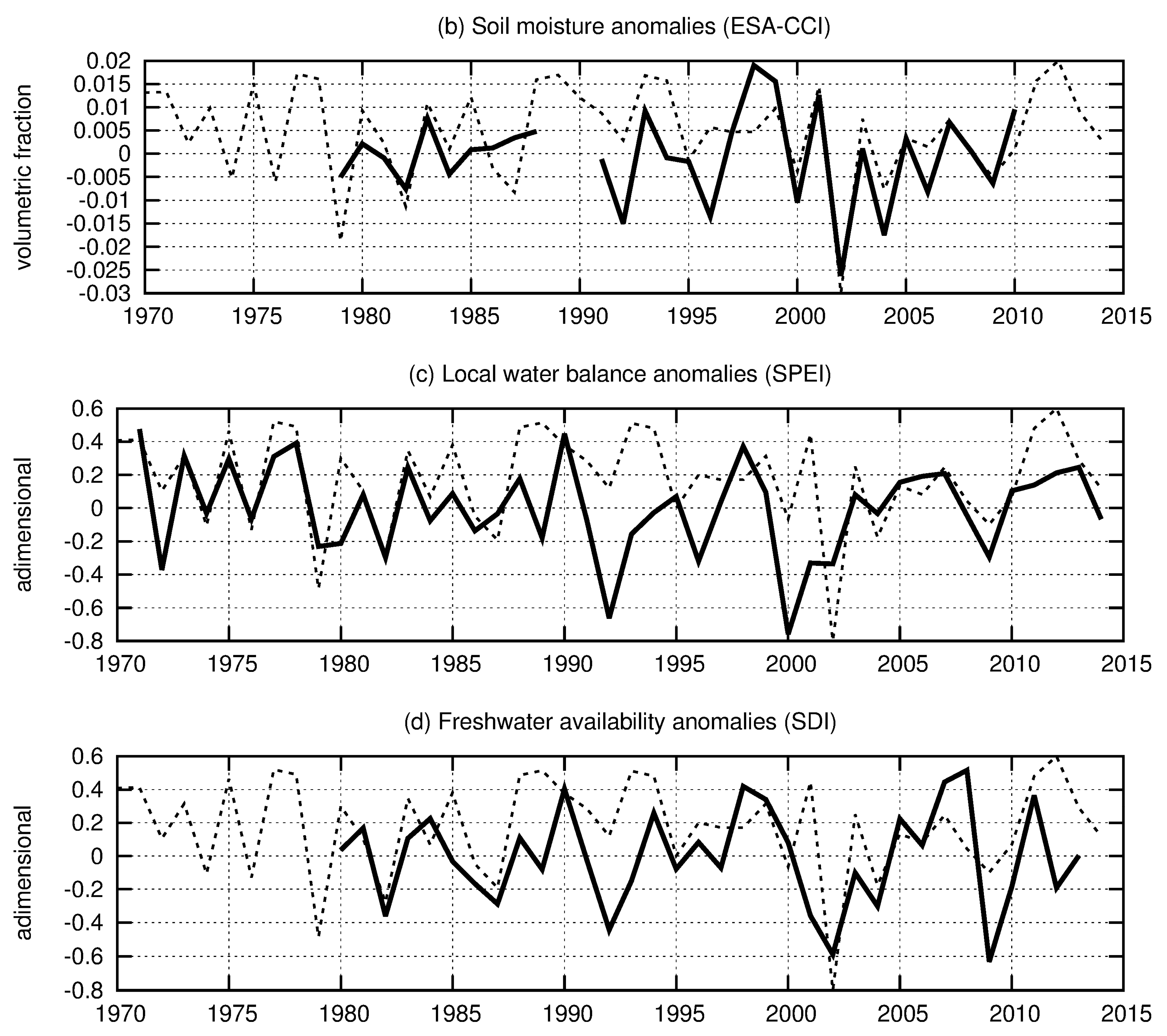
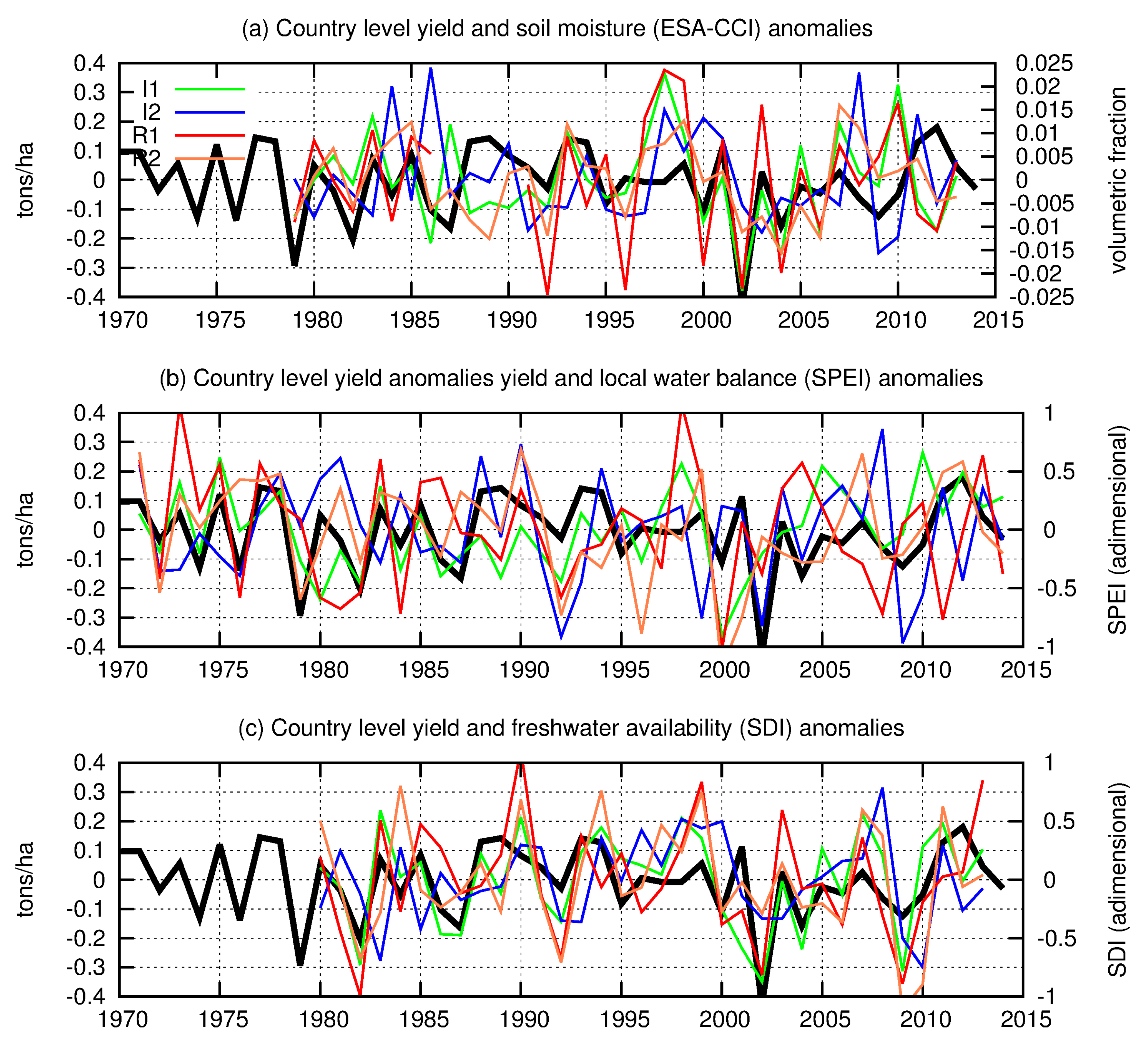
  • the ESA-CCI soil moisture index [22], computed on remotely sensed measurements of near surface soil moisture (i.e., the few top centimeters), here considered as the observational reference;
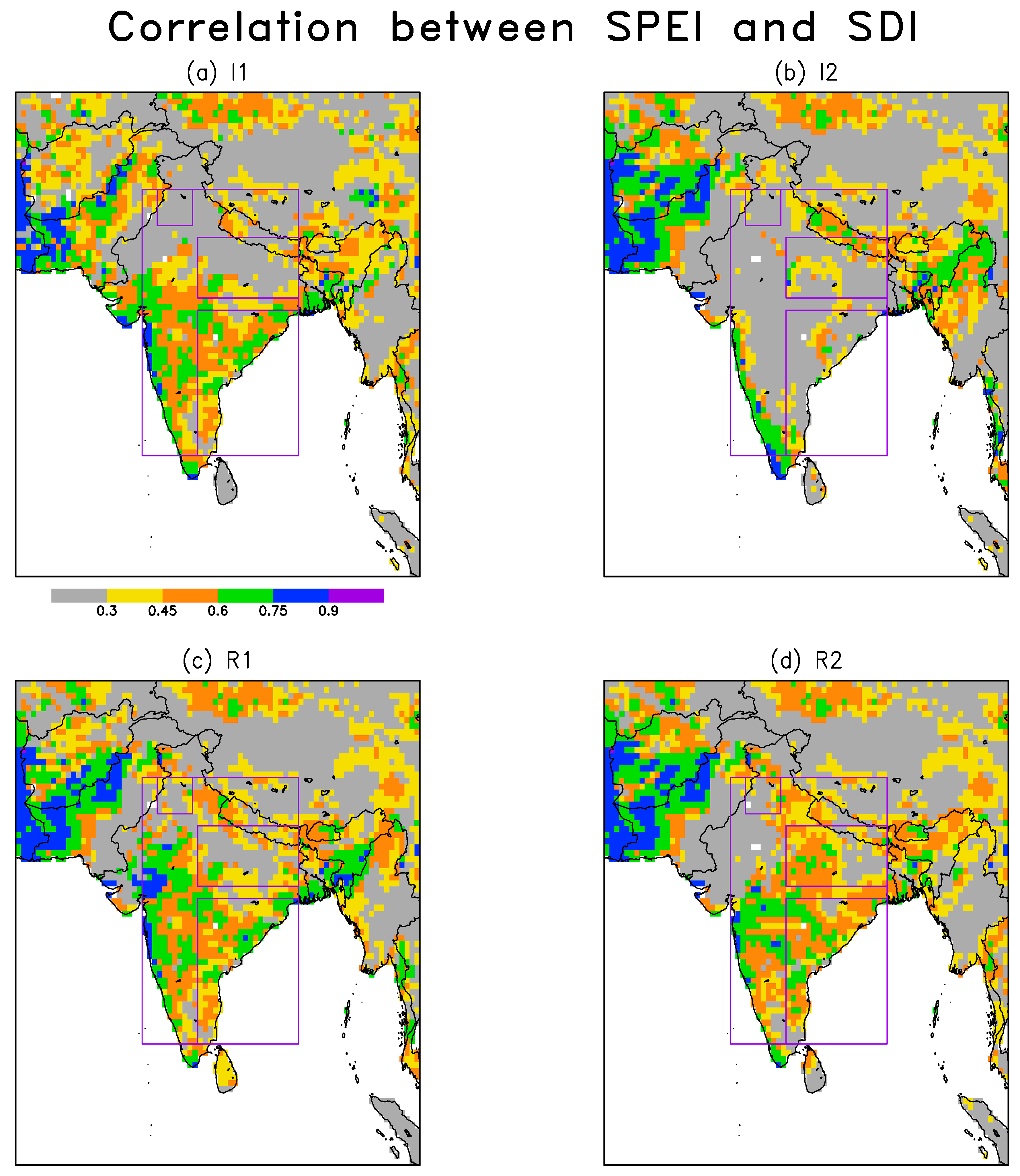
  • the standardized precipitation evapotranspiration index (SPEI [21]), as a proxy for the soil moisture anomalies given by the local soil water balance (i.e., precipitation minus evapotranspiration);
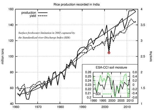
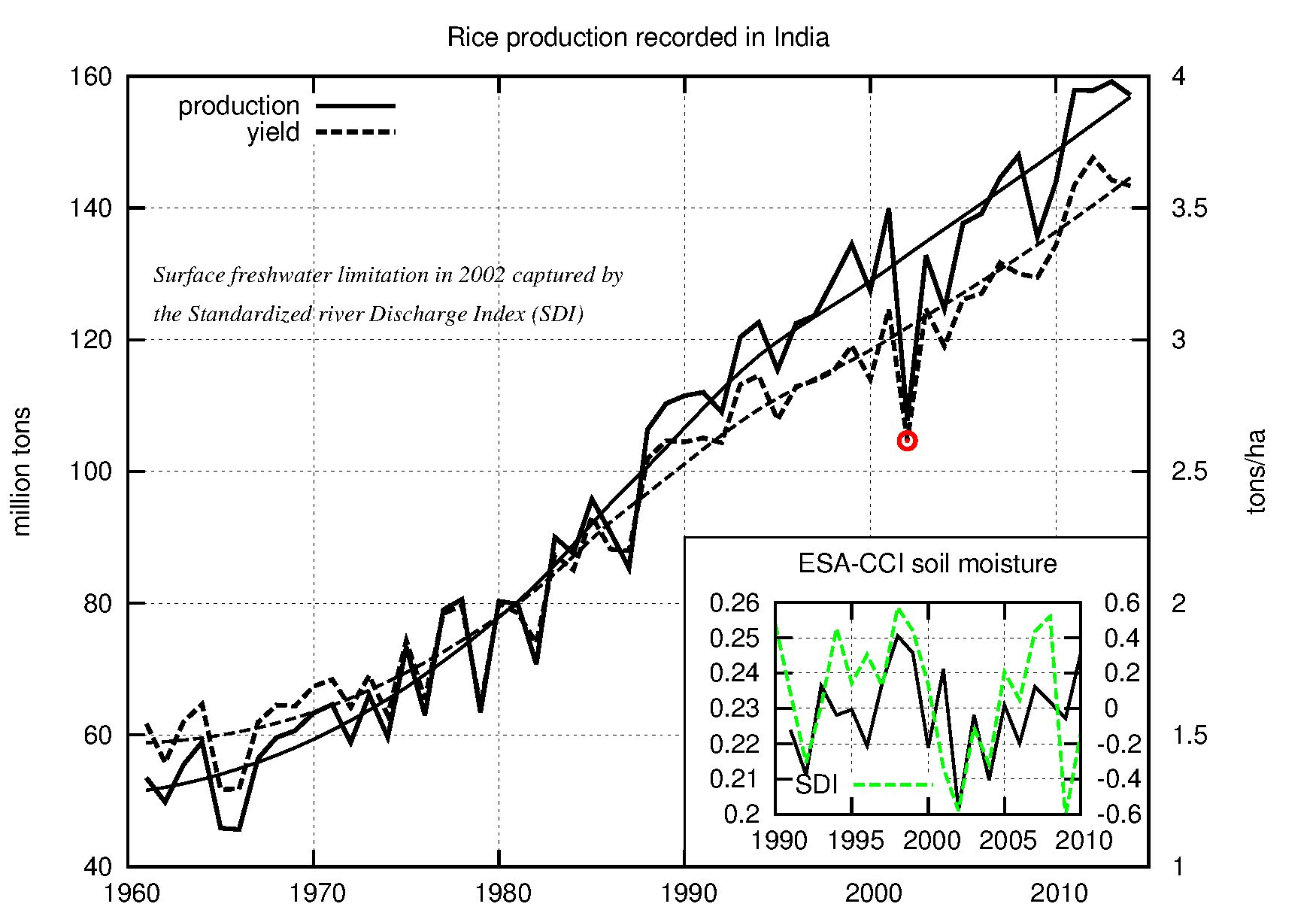
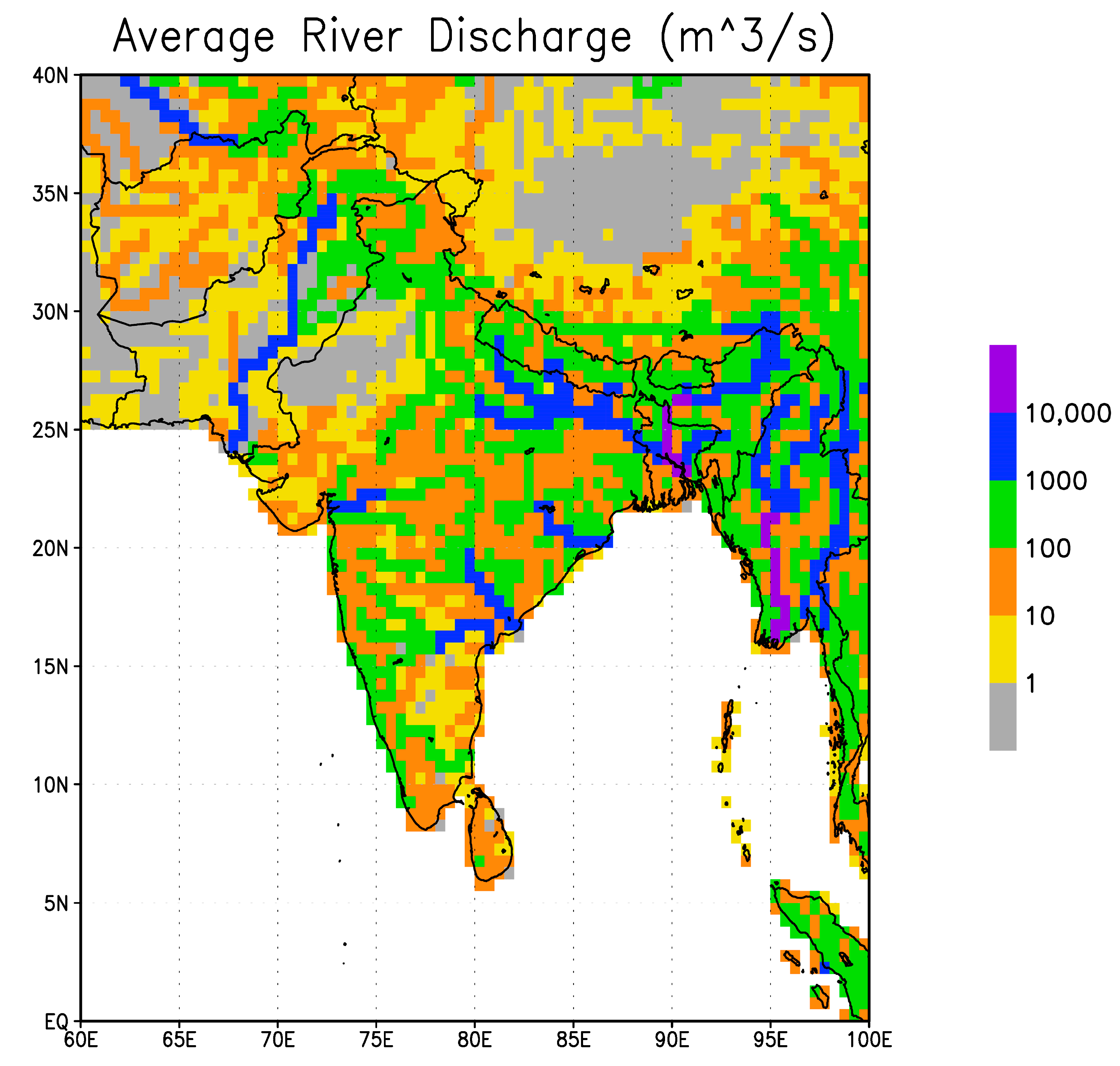
  • the standardized river discharge index (SDI, this study), as a proxy for the anomalies of water available for irrigation and paddy field flooding, here assumed to be related to the river discharge originated by the upstream runoff.
We perform the analysis in a time window covering the period from 1980 to 2014, with a specific emphasis on 2002 at both the national and regional level. At the national level, we compare the long-term FAOSTAT annual yield time-series [23] with the indicators averaged over all cropping cycles, as in [20]. Moreover, we disentangle the main cropping cycles in order to identify the ones more affected by the 2002 drought, and the process indicator (i.e., the local SPEI vs. the non-local SDI) that is more closely reproducing the yield and the ESA-CCI observed anomalies with respect to the baseline trend.
At the regional level, we characterize the spatial variability of the 2002 drought as given by the ESA-CCI soil moisture and by the local and non-local hydro-climatic indexes at the monthly time scale. The regional analysis is discussed in comparison with the production statistics at the state level around year 2000 obtained from the Indian Ministry of Agriculture [9].

2. Materials and Methods

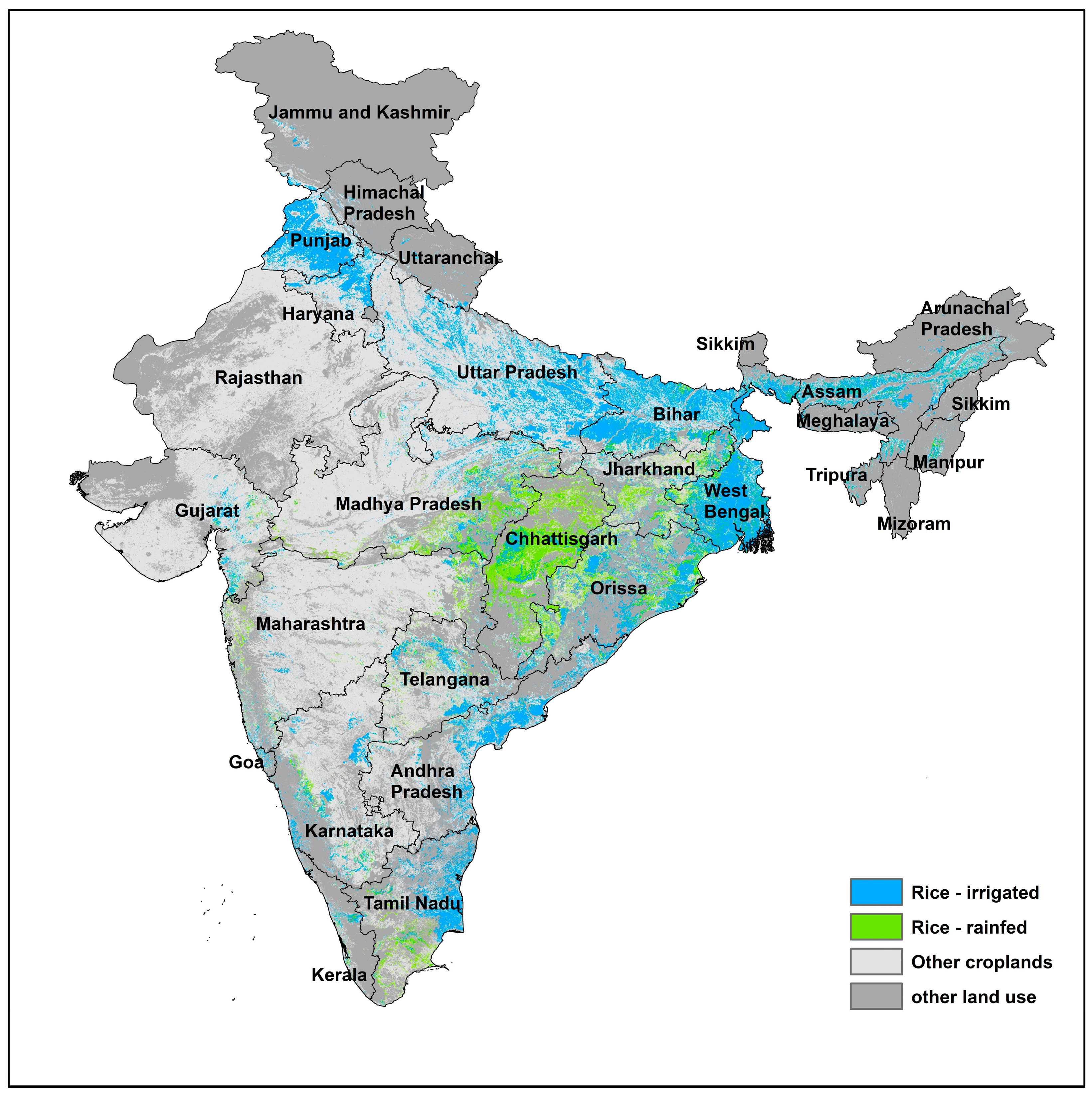
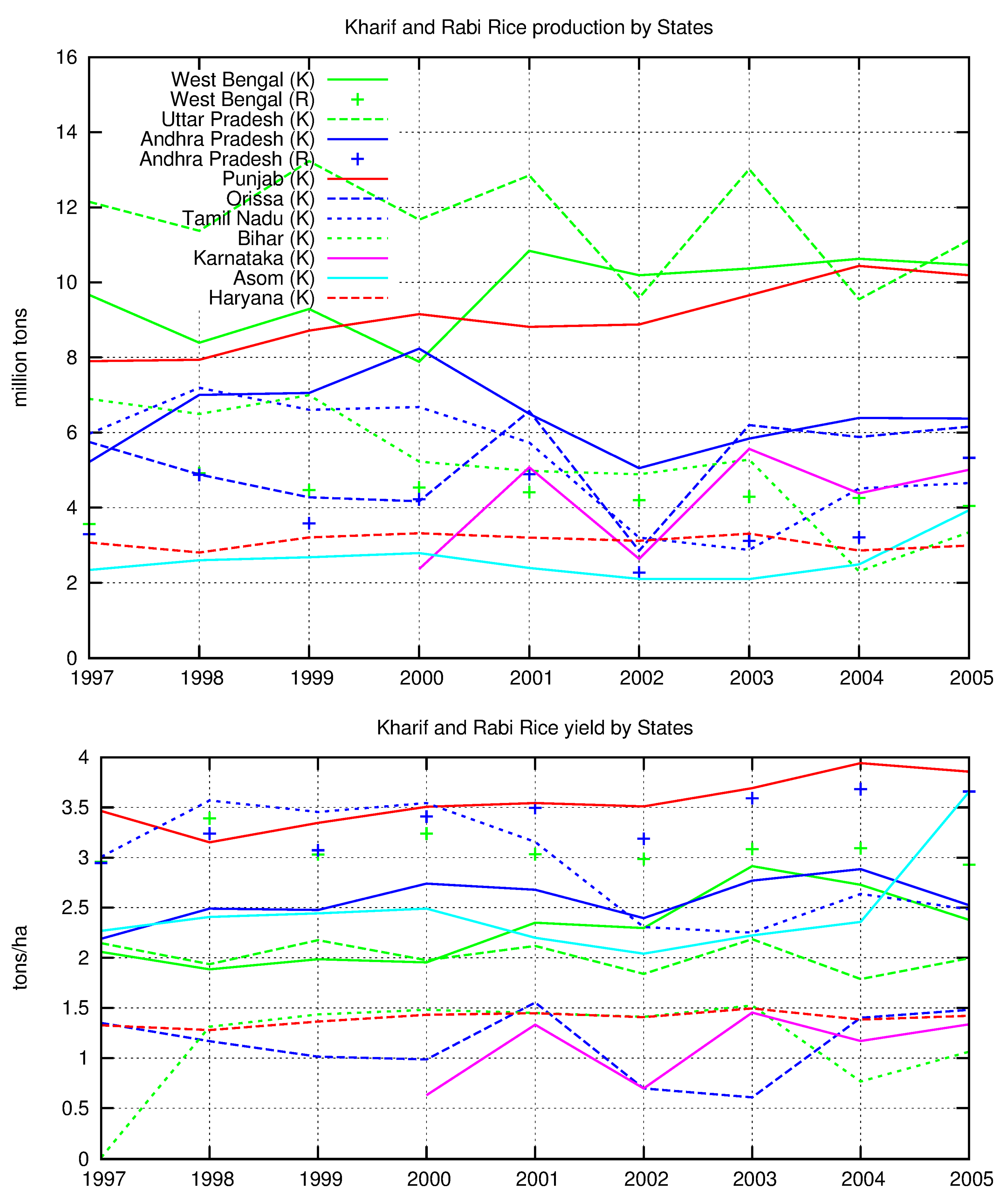
2.1. Rice Cropping Pattern in India

The reference rice cropping map (Figure 1) was extracted from a MODIS-derived rice extent map [1,2], consisting of eight rice classes with a classification accuracy of 82% and 84% agreement with rice areas from state statistics. This rice extent map is the most detailed publicly available map for India.
In India, rice is harvested up to three times per year during the Kharif (monsoon) season, from June to August, the Rabi season, from October/November to January/February, and in summer, starting on February [1,2].
As in [20], we adopt the MIRCA2000 global cropping calendar dataset [4] (Figure 2). MIRCA2000 classifies the rice plantations in four main cycles, three of which are associated with the Kharif rice cycle and one is either the Rabi or summer rice cycle. MIRCA2000 provides the spatial distribution, planting month, and harvesting month for each rice cropping cycle (see Figures S1 and S2). Some of them are coexisting in the same location at the same time and are distinguished by areas equipped with irrigation and lowland flooded areas that are classified as rainfed [4] (mainly located in the eastern States of India, consistently with [1,2], see Figure 1).
The total rice areal extension reported by MIRCA2000 (i.e., 39.1 million hectares around year 2000) is comparable with the 44.7 million reported by FAOSTAT in 2000. According to MIRCA2000, about half of the rice production areas (20.0 million hectares) are irrigated while the other half are rainfed (18.8 million hectares). Irrigation is mostly based on groundwater rather than surface water withdrawals in Punjab and Haryana in the northwest. Groundwater withdrawals also occur for a significant fraction of the total irrigation (i.e., 30% to 80%) in the Ganges basin. While they are negligible in the rest of India (see Figure S3).
The harvested area given by MIRCA2000 (Figure 2) is used for the weighted averages of the hydro-climatic indicators at the national and regional levels (see Section 2.6). The harvesting month information from MIRCA2000 is used to determine the preceding period when the crop is more sensitive to climate anomalies (Figure S2). Thus, the climatic indicators are computed over these periods, which vary for each cropping cycle. Below the two irrigated rice cycles (I1 and I2) and the two rainfed cycles (R1 and R2) are defined.
Following the monsoon dynamics, Kharif rice is grown from April in the east and from June in the center to the end of the year in irrigated fields (I1 cycle, Figure 2a, 11.2 million hectares) and in rainfed/flooded lowlands (R1 cycle, Figure 2c, 6.9 million hectares; R2, Figure 2d, 11.9 million hectares). The two different rainfed cycles (R1 and R2) are characterized by different harvesting dates. The second irrigated cycle (I2, Figure 2b, 9.2 million hectares) roughly corresponds to Rabi rice and it is responsible for about 10% of the production around 2002 [9].

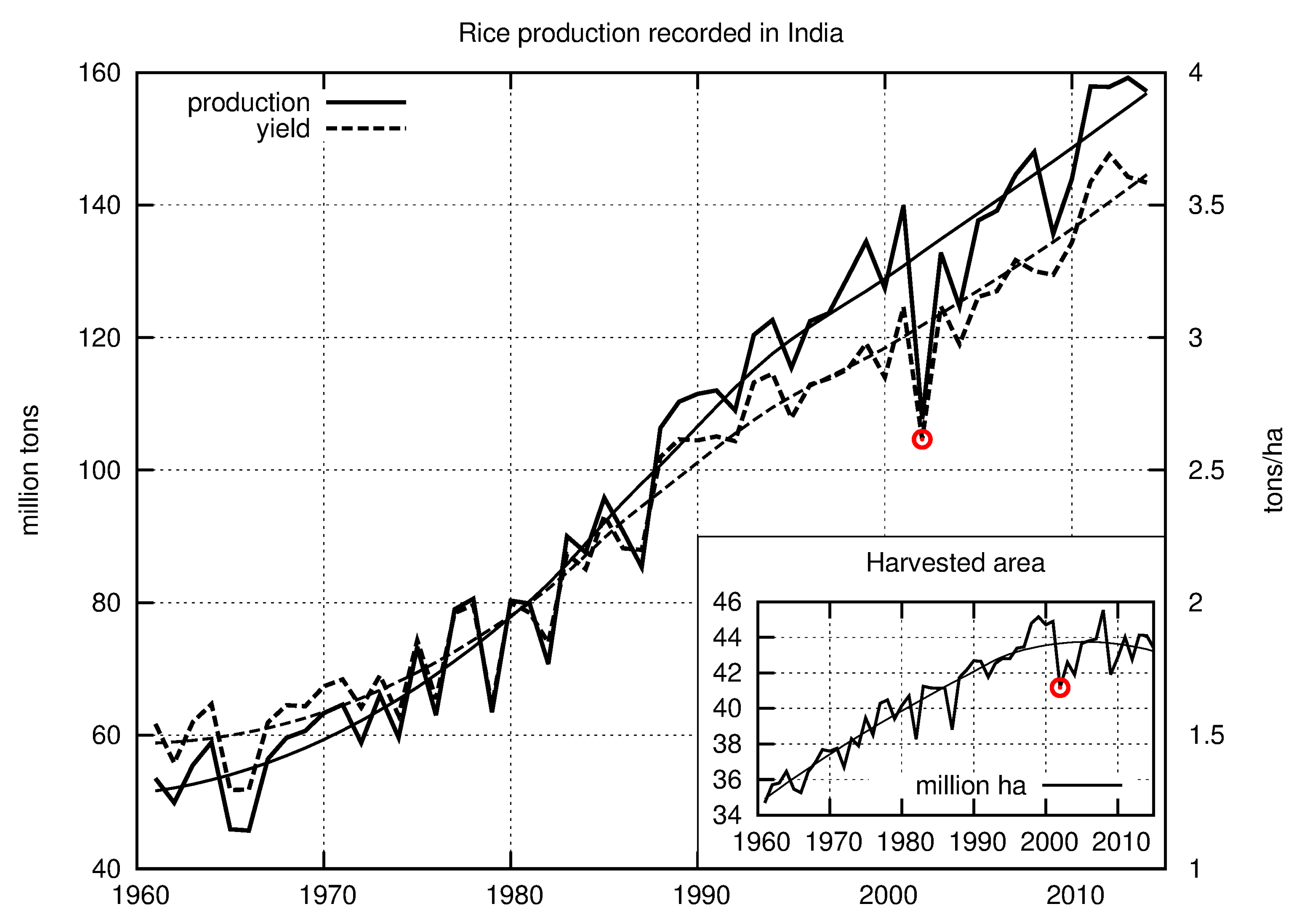
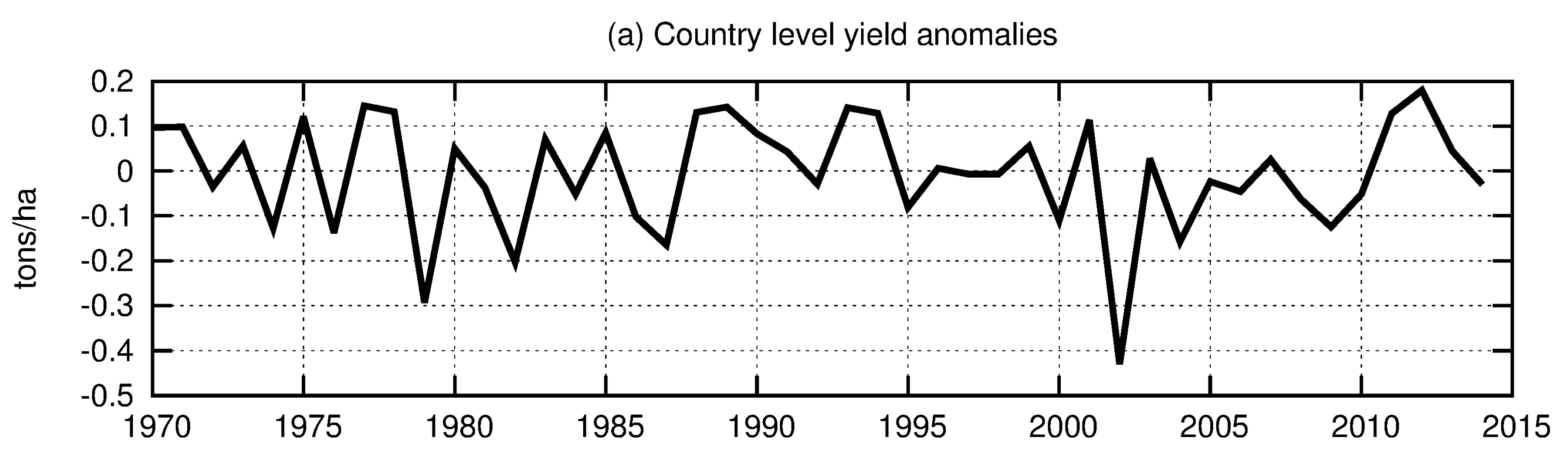
2.2. Agricultural Data

Rice yield and production data have been obtained from FAOSTAT [23] and are available from 1961 to 2014. These data are shown in Figure 3. The anomalies with respect to the baseline (i.e., fitted long-term trend in Figure 3) are compared with the agro-climatic indicators, presented in Section 3.1. Pearson two-sided test is used to quantify the statistical significance of the computed linear correlations.
At the national level, Indian rice production has increased by a factor of three from about 50 million tonnes in the early 1960s to more than 150 million tonnes after 2010 (Figure 3), mostly consumed for domestic supply [23]. During this period, population has proportionally increased at a factor of 2.9, passing from 450 to 1300 million [23]. The production increase is mostly due to the yield increase, but also to the increase in the areas devoted to rice cultivation and the multiple cycles (see inset in Figure 3).
The national annual rice production baseline (i.e., the fitted long-term trend in Figure 3) surpassed 130 million tonnes around year 2000, but the actual production decreased in 2002 to 107 million tonnes, i.e., the value recorded 10 years earlier. The 2002 production anomaly corresponds to a decline of 18.9% with respect to the baseline value for 2002 (see Figure 3), 4.5 times larger than the inter annual production standard deviation of the anomalies recorded in the 1997–2007 period, and the largest during the observational period (1960–2014) in both absolute and relative terms.
The 2002 yield (i.e., production divided by area) anomaly is equal to 14.1% of the baseline value, corresponding to five times the standard deviation. The proportionally larger production drop versus yield is consistent with the lower areas classified as harvested in 2002 (see inset in Figure 3), likely because of total yield loss.
Agricultural records at the State level are generally not available. However, we have retrieved a report of the Directorate of Rice Development of the Indian Agricultural Ministry with data covering the year 2002, distinguishing between Kharif and Rabi rice production and yields for each Indian State [9]. We digitized those data and use them to strengthen the discussion of our analysis at the regional level in Section 3.2.

2.3. Soil Moisture Observations

Satellite soil moisture retrievals have been often used to diagnose drought and soil moisture anomalies, especially in irrigated areas [25] and in river flow-driven inundated floodplains [26], also for India [27]. Here, we adopt the ESA-CCI soil moisture dataset, combining multiple active and passive sensors [28]. ESA-CCI is available at a resolution of 0.25° globally, spanning the years from end of 1978 to 2014, with gaps.
The ESA-CCI soil moisture data set has been used to evaluate soil moisture trends at the global [28] and regional scale e.g., over the Tibetan Plateau [29]. The ESA-CCI soil moisture has already been extensively validated over the India continent as well [30,31,32,33]. In particular, the ESA-CCI product merging active and passive sensors that is used in this study is in good agreement (i.e., high Pearson correlation coefficients) with the soil moisture time-series produced by both the land surface reanalysis and the high-resolution precipitation data [30,32] in India. ESA-CCI has been evaluated also with the available direct soil moisture observations in India, providing similar correlations coefficients with respect to reanalyzed soil moisture datasets [31]. The ESA-CCI ability to detect agricultural drought specifically has been assessed as well using vegetation indexes from satellite and crop yields at the district level in the Rabi season [34]. Therefore, we use the ESA-CCI as validation for the other indexes.

2.4. Local Soil Moisture Proxy

Soil moisture can be estimated through the standardized precipitation–evapotranspiration index SPEI [21]. The SPEI is computed from gridded precipitation and temperature datasets derived from station observations at monthly time-scales, it is integrated from 1 to 24 months ahead and is available on a global 0.5° grid for the period 1901–2014. The SPEI allows the comparison of the surface water balance anomalies with respect to the local climatology in different locations. The SPEI is a well-accepted indicator for soil moisture drought. It is significantly correlated with vegetation indexes in India (r = 0.4–0.8) on a characteristic time scale of three months or less [21]. The SPEI has been already used to characterize agricultural drought in India (Ganges region) where it has been found to be significantly correlated with cereal yield losses (r = 0.69) [35]. However, it neglects any other possible non-local influences on soil moisture, such as irrigation, which might be particularly relevant for rice fields.

2.5. Non-Local Freshwater Availability

For each grid point, we assume that available freshwater is linked to a non-local component of the surface hydrology, i.e., the runoff accumulated and aggregated in the basin upstream. The water amount that is actually available locally is derived from a river discharge model simulation conducted with the Global Flood Awareness System (GloFAS [36,37]). GloFAS is composed by a land surface model (HTESSEL [38]) and the LISFLOOD gridded river routing model [39]. The simulation used here is driven by meteorological fields derived from reanalysis (ERA-Interim [40]), starting in 1980, and it is validated using local river discharge observations (where available).
The soil moisture component of the GloFAS system is significantly correlated to the ESA-CCI product in India (r > 0.5) [33]. The GloFAS river discharge has been validated in the Indian region [36], proving to have significant forecasts skills as in the case of the 2010 flood of the Indus basin. The river discharge adopted here, being produced by a model simulation forced by meteorological observations rather than forecasts, can be considered a realistic indicator of the runoff generated upstream.
The original 0.1° high-resolution data were scaled-up to 0.5° for comparison with the other data sets (see Figure 4). Indeed, the lower resolution corresponds to the relevant spatial scales characterizing river-soil moisture interactions [41,42] and it is adopted also in other irrigation water demand studies [43,44,45]. The specific time-scale of the SPEI and SDI chosen for this study is three months prior to the harvesting month for each cropping cycle (see Section 2.1). This choice, resulting from a preliminary sensitivity study (not shown), is giving for all the indicators the highest correlation with the FAOSTAT national yield anomalies time-series.
The GloFAS, in the present configuration, does not consider water withdrawals from irrigation or other sources. Therefore, the SDI has to be considered as an indicator for the variability of available freshwater rather than an accurate component of the water balance.
Figure 4 shows the multi-annual averaged river discharge data from the GloFAS simulation at 0.5° × 0.5° horizontal resolution. Most of India, except the desert in Rajasthan, is covered by rivers of variable size [6,7]: the Indus in the northwest, flowing into Pakistan; the Ganges in the northeast, merging with the Brahmaputra in Assam and Bangladesh; the Narmada in the West, the Mahanadi, the Godavari, and the Krishna in the East. The Indus and Ganges basins are separated by the Thar Desert, also known as the Great Indian Desert, which forms a natural boundary between India and Pakistan. Some of the rivers flowing through Haryana (the State of New Delhi) dry up in the Thar Desert, never reaching the sea or merging with other rivers. A complex network with 10 to 1000 m3/s discharge occupies most of the Indian Peninsula, flowing preferentially from west to east. The water taken up from rivers is distributed into paddy fields through a dense net of artificial channels [1,2,6,7], and stored in artificial ponds [6,7].
In order to compare the freshwater anomalies in different locations, characterized by the presence of rivers of different sizes and different seasonal cycles, we define a standardized index also for the non-local water transport, i.e., the standardized river discharge index (SDI). The SDI is computed exactly in the same way as the SPEI i.e., for each month and location using log-logistic probability density functions [21] (see Supplementary Material). Compared to the SPEI, the SDI is based on monthly river discharge data from the GloFAS simulation instead of the precipitation and potential evapotranspiration difference.
Figure 5 shows the estimated linear correlation coefficients between the SPEI and the SDI. For relatively small or not significant correlation coefficients, the information content of the SDI is mostly non-local. Regions with few upstream catchment areas and intense precipitation, as the western coastal part of the Peninsula, are characterized by higher linear correlations, reflecting the fact that the river discharge is mostly a result of the local runoff (thus closely related to the SPEI). On the other hand, during the Rabi/summer irrigated cycle (I2), the SDI is almost entirely decoupled from the SPEI.

2.6. Computation of Annual Time-Series at Country Level

Summarizing, the main steps of the implemented procedure for the annual time-series analysis at country level are:
  • all gridded datasets are interpolated onto a 0.5° × 0.5°common grid;
  • the indexes are computed over period when the crop is more sensitive to climate anomalies independently for each cropping cycle (i.e., three months from harvesting as given by the MIRCA2000 dataset, see Section 2.1, Figure S1);
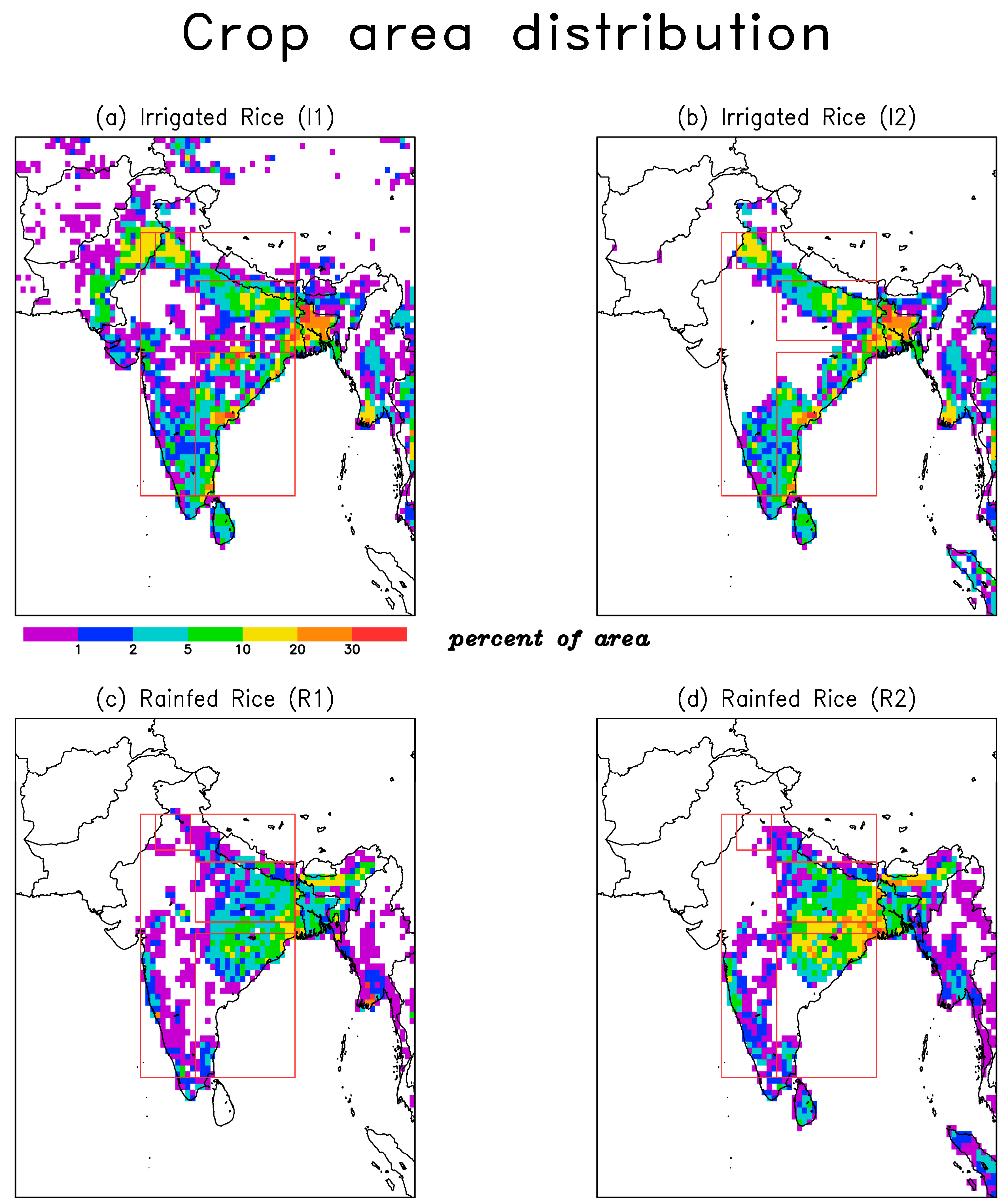
  • when different cropping cycles are present in the same grid, weighted averages are computed using the relative contribution to the total harvested area as given by the MIRCA2000 dataset (Figure 2);
  • aggregations at the national (and regional) level are computed by using again the MIRCA2000 harvested area as weighting factor;
  • LOESS detrending is performed to compare the indexes with the yield anomaly time-series from FAOSTAT.
Missing numbers are not present in the SPEI nor in the SDI gridded product, but they can affect satellite observation datasets. We attribute missing values to the spatial averages computed in the years when less than 50% of fields (weighted by the harvested area) is covered for each cropping cycle. This leaves uncovered the R1 cycle from 1987 to 1991. Complete time-series since 1979 are obtained in the other cases. When aggregating all cropping cycles, the years 1988–1990 are considered as missing values.

3. Results

3.1. National Level Analysis

Figure 6 shows the anomalies of yield (as in Figure 3) and soil moisture anomaly indicators after removing a non-linear long-term trend.
The ESA-CCI soil moisture product (Figure 6b) is clearly capturing the 2002 anomaly, and it is also significantly correlated with the entire yield anomalies time-series (r2 = 0.43, computed on all valid data).
The SPEI (Figure 6c) is also significantly correlated with the yield anomalies, albeit explaining lower variance fraction (r2 = 0.11). Notably, it largely underestimates the impacts of drought on production in 2002. The local SPEI index would have predicted the worst conditions in 2000, which was actually characterized by nearly normal yield and small ESA-CCI soil moisture anomalies.
In contrast, the SDI (Figure 6d) is somewhat better correlated (r2 = 0.19) with the yield with respect to the SPEI, suggesting a role on the non-local water dynamics for rice yields. Most importantly, the SDI captures the 2002 event. Notably, the preceding year was also relatively surface freshwater poor (i.e., low SDI). Note that the SDI would have also predicted dry conditions in 2009, which was actually characterized by smaller yield anomalies and drought conditions as given by the ESA-CCI soil moisture. 1982 and 1992 were also characterized by large, but moderate, freshwater availability issues. A consistent soil moisture anomaly is diagnosed by the ESA-CCI retrieval, but it did not correspond to a large yield loss as in 2002. The increased susceptibility of 2002 with respect to 1992 is probably due to more intense cropping pressure (see the harvested area time-series in Figure 3).
Disentangling the four cropping cycles provides a more detailed characterization of the 2002 drought event.
Soil moisture remotely sensed observations (ESA-CCI, Figure 7a) clearly identify 2002 as the worst drought event in the records for primary irrigated and rainfed cycles (I1 and R1). In 1992, only the rainfed cycle (R1) was affected and the same happened in 1996, 2000, and 2003.
The SPEI (Figure 7b) captures some of the drought events diagnosed by the satellite product for the rainfed cycles. Interestingly, the river-drought years (e.g., 1992, 2002 and 2009) were anticipated by a meteorological drought (e.g., diagnosed by the SPEI) during the secondary rainfed cycle (R2), harvested earlier in the Rabi/summer season.
The SDI (Figure 7c) captures the 2002 event for the primary Kharif irrigated and rainfed cycles (R1 and I1), consistently with the ESA-CCI retrieval (top panel). 1992 was characterized by a moderate river drought, affecting mostly the rainfed cycles and the irrigated ones to a lesser extent. The SDI would have predicted negative yield anomalies for three cycles in 2009. However, the preceding year was relatively surface freshwater rich (i.e., high SDI).
Table 1 shows the linear correlations among the time-series shown in Figure 7. Overall, all indicators are significantly correlated in all cropping cycle, with the exception of the SPEI during the R2 cycle. The SDI always displays the largest correlations with the ESA-CCI soil moisture retrievals.

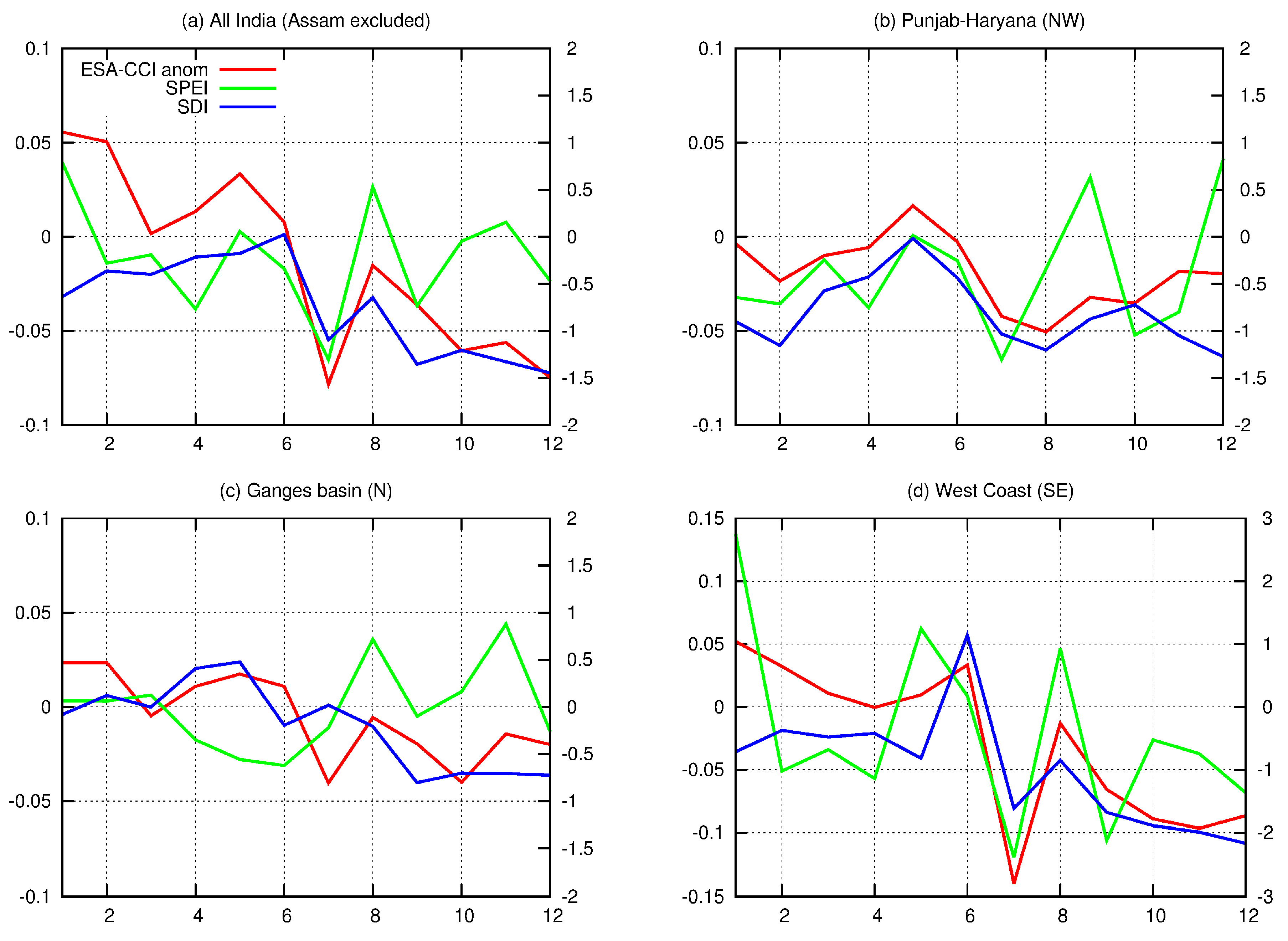
3.2. Regional Level Analysis

Figure 8 (top panel) shows the time-series of rice production at the state level, for the top 10 Indian producers [9]. Some of the main producers of Kharif rice are responsible for the total 2002 anomaly: Uttar Pradesh, located in the Ganges basin; all states located on the southeastern coast (especially Andhra Pradesh, for both Kharif and Rabi rice); Karnataka, located in the south western coast. West Bengal, located in the Ganges–Brahmaputra delta, and Punjab, located in the northwest, show small anomalies.
The visual inspection of the yield time-series immediately highlights the marked intensity of rice cropping during the Kharif period in Punjab and during the Rabi irrigated cycles in Andhra Pradesh and West Bengal.
Figure 9 shows the 2002 monthly anomalies of all indicators aggregated over all rice production areas for the regions depicted in Figure 2 and Figure 5. At the Indian continental scale (Figure 8a) a decrease of soil moisture was observed in rice cropping regions, passing from above normal to below normal conditions. This constant inter-seasonal trend is captured by the SDI, but not by the SPEI that mainly reflects the July precipitation anomaly [14,15,16].
The Punjab–Haryana region (Figure 9b) also shows drier than normal conditions in the satellite and river discharge data for the second part of the year. This region recorded limited effects on the yield though (see Figure 8), probably because of the dominant use of groundwater for irrigation.
The Ganges basin (Figure 9c) shows similar conditions. Albeit employing significant groundwater withdrawals, this region was hardier affected in term of rice yield in 2002 (see Figure 8). The above-normal precipitation recorded in August and November did not alleviate the effects of the previous drought.
The southeastern coastal regions (Figure 9d) are adopting irrigation from surface water only and show the more intense drought that, again, was only limitedly alleviated by the above-normal precipitation recorded in August.
Table 2 shows the linear correlations among the time-series shown in Figure 9. With respect to the SPEI, the SDI displays the larger and more significant correlations with the ESA-CCI soil moisture monthly variations for each region. The time-series of SPEI and SDI are poorly correlated.

4. Discussion

Lack of irrigation played a crucial role in the case of the exceptional 2002 negative production anomaly in India. The 2002 anomaly was five times the interannual standard deviation large and roughly equivalent to 10 years of progress in the yield and production amounts. This kind of unfavorable condition is critical for the constantly growing Indian population, as it might happen again and more frequently in the context of global warming [44,46]. In fact, India has been identified as the third country exposed to the higher water risk for agriculture in future scenarios after China and the USA [47].
In case of dry conditions, while irrigation is often invoked as the main strategy to maximize yields and to adapt to the effect of climate change, the water available may increasingly become a limiting factor. Adaptive capacity limitation due to variable freshwater availability should be accounted in the crop models used to simulate yield changes in future climate change scenarios [43,44,45].
In this study, we have characterized the role and the contribution of the non-local surface freshwater component by defining a new indicator, i.e., the standardized river discharge index (SDI). Assuming that surface freshwater availability is proportional to the runoff upstream to the rice fields, the new indicator is based on river discharge data obtained from a gridded hydrological model.
The general idea is not new, as it bears some resemblance with the standardized runoff index (SRI [48]), computed on local runoff resulting from the balance between precipitation and evapotranspiration. The SDI, being computed on the actual river discharge, is considering the non-local surface water transport from runoff generated at long distances as well. Moreover, the SDI takes the orographic factors into account; i.e., the fact that precipitation and snowmelting are mainly localized in the mountainous regions, while crops are grown in the plains downstream.
A comparison with the SRI computed with the runoff data used in the GloFAS system to simulate the river discharge is presented in the Supplementary Material (Table S1, Figure S4). In general, the SDI is better correlated with the SRI than with the SPEI, which is expected because the runoff is the source of water for the rivers. The SRI is better correlated than the SPEI to the observations (i.e., the ESA-CCI soil moisture), meaning that the runoff at the grid level is a better indicator of soil moisture anomalies than the SPEI in irrigated regions. However, the SDI is still delivering the best performance, meaning that the non-local component is important at spatial scales larger than the grid cell (0.5 degrees in this study). The only partial exception to the abovementioned statement is for the I1 cycle, the most frequent in the Punjab region. In this region, irrigation is mainly based on groundwater, which is neglected in our analysis.
The main findings of this study help shed some light on the related processes affecting soil moisture and water availability in agricultural areas. Moreover, they strongly confirm the value of satellite surface soil moisture retrievals in irrigated regions. Albeit the analysis is based on a generally accepted statistical framework [20], a precise complete characterization of the associated uncertainties is still missing. However, all the datasets here used have already been extensively validated for India (see discussion in Section 2.4, Section 2.5 and Section 2.6).
In general, we have noted some spatial inequalities in the strength of the dryer-than-usual effects on yield. For instance, the rich and developed Punjab and Haryana States, where irrigation is largely based on non-renewable groundwater exploitation [49,50], were less affected. It is interesting to note that, probably because of the higher productivity, climatic impact assessment studies often address these two regions only [47].
Results show some limitation in predicting the effects of the moderate 2009 dry anomaly, characterized by sub-optimal, but not exceptionally low yield. In fact, the non-local surface freshwater availability index would have anticipated a drought similar to the one in 2002. However, 2002 was preceded by a dry year, which probably affected the surface and groundwater reservoirs.
Moreover, it has been suggested that rice production systems adapted in response to the 2002 event and to the general increase in water scarcity in the southeastern coastal regions [51]. Drought resistant rice varieties have been introduced along with more limited flooding practice [51], targeted agricultural water management interventions [52], cropping pattern change [18,53,54], and other forms of adaptation at the farmer level [55]. These adaptation measures are likely reflected in the sensitivity of country level yield and production on climate anomalies.

5. Conclusions

We have analyzed the hydrological conditions during the 2002 record-low year for rice production in India, using satellite soil moisture retrieval (ESA-CCI), a proxy of the local water balance (SPEI), and a newly defined non-local indicator of surface water availability for irrigation and paddy field flooding (SDI). The soil moisture anomalies computed with the ESA-CCI data are well correlated with the yield anomalies (r2 = 0.43). The comparison between the SPEI and the SDI and their correlation with yield anomalies (r2 = 0.11, r2 = 0.19) suggest that the non-local component is the more important driver of the soil moisture anomalies in rice fields.
Including non-local hydrology, as represented by a gridded river discharge model, is essential to capture the observed yield and soil moisture anomalies, and therefore to better characterize the processes underlying the effects of the 2002 extreme drought on yields. Thus, the new proposed indicator represents a potentially useful tool for predicting the risk of occurrence of similar agricultural droughts in the future, both in the context of seasonal forecasts and climate change projections.
The effects of the 2002 drought varied regionally. Regions using groundwater supplies for irrigation, albeit non-sustainable, were less affected (e.g., Punjab). After the 2002 event, other more affected regions (e.g., Orissa) have adapted cultivation practices to save water.
A more advanced and higher resolution hydrological modeling system, including water withdrawal by agriculture, and rice in particular, would be needed to understand the risks and adaptation needed with regard to changing climate and climate variability. Satellite observations of soil moisture can provide opportunities for the calibration of those models.
Finally, our findings further demonstrate the value of near-real-time soil moisture retrievals from satellite observations to assess the current state of rice paddy fields, providing near-term information on immediate water management options.

Supplementary Materials

The following are available online at https://www.mdpi.com/2072-4292/10/2/244/s1, Figure S1: Rice planting dates, Figure S2: Rice harvesting dates, Figure S3: Maps of percentage of areas equipped for irrigation (and percentage of areas equipped for irrigation with groundwater. Figure S4: Time-series of standardized runoff index (SRI), Table S1: Correlation analysis of soil moisture indicators, including the SRI.

Author Contributions

Matteo Zampieri, Gema Carmona Garcia, Frank Dentener, and Andrea Toreti conceived and designed the experiments; Peter Salamon and Murali Krishna Gumma provided data; Matteo Zampieri and Lorenzo Seguini analyzed the data; Matteo Zampieri and Andrea Toreti wrote the paper. All authors substantially revised the paper.

Conflicts of Interest

The authors declare no conflict of interest.

References

  1. Gumma, M.K.; Thenkabail, P.S.; Teluguntla, P.; Rao, M.N.; Mohammed, I.A.; Whitbread, A.M. Mapping rice-fallow cropland areas for short-season grain legumes intensification in south asia using modis 250 m time-series data. International. J. Dig. Earth 2016, 9, 981–1003. [Google Scholar] [CrossRef] [Green Version]
  2. Gumma, M.K.; Nelson, A.; Thenkabail, P.S.; Singh, A.N. Mapping rice areas of south asia using modis multitemporal data. J. Appl. Remote Sens. 2011, 5, 053547. [Google Scholar] [CrossRef]
  3. Palazzi, E.; von Hardenberg, J.; Provenzale, A. Precipitation in the Hindu-Kush Karakoram Himalaya: Observations and future scenarios. J. Geophys. Res. 2013, 118, 85–100. [Google Scholar] [CrossRef]
  4. Portmann, F.T.; Siebert, S.; Döll, P. MIRCA2000—Global monthly irrigated and rainfed crop areas around the year 2000: A new high-resolution data set for agricultural and hydrological modeling. Glob. Biogeochem. Cycles 2010, 24, GB1011. [Google Scholar] [CrossRef]
  5. Pekel, J.-F.; Cottam, A.; Gorelick, N.; Belward, A.S. High-resolution mapping of global surface water and its long-term changes. Nature 2016, 540, 418–422. [Google Scholar] [CrossRef] [PubMed]
  6. JRC Global Surface Waters Explorer. Available online: https://global-surface-water.appspot.com/ (accessed on 22 September 2017).
  7. Biggs, T.W.; Scott, C.A.; Gaur, A.; Venot, J.-P.; Chase, T.; Lee, E. Impacts of irrigation and anthropogenic aerosols on the water balance, heat fluxes, and surface temperature in a river basin. Water Resour. Res. 2008, 44, W12415. [Google Scholar] [CrossRef]
  8. De Vrese, P.; Hagemann, S.; Claussen, M. Asian irrigation, African rain: Remote impacts of irrigation. Geophys. Res. Lett. 2016, 43, 3737–3745. [Google Scholar] [CrossRef]
  9. Directorate of Rice Development of the Indian Agricultural Ministry. Available online: http://drdpat.bih.nic.in/Downloads/Handbook-of-Statistics-2007.pdf (accessed on 19 October 2017).
  10. India Meteorological Department, Ministry of Earth Science. Available online: http://www.imd.gov.in/pages/monsoon_main.php (accessed on 5 November 2017).
  11. World Bank. Available online: https://data.worldbank.org/ (accessed on 10 October 2017).
  12. FAO; IFAD; WFP. The State of Food Insecurity in the World 2015. Meeting the 2015 International Hunger Targets: Taking Stock of Uneven Progress; FAO: Rome, Italy, 2015; Available online: http://www.fao.org/3/a-i4646e.pdf (accessed on 3 November 2017).
  13. Hallegatte, S.; Bangalore, M.; Bonzanigo, L.; Fay, M.; Kane, T.; Narloch, U.; Rozenberg, J.; Treguer, D.; Vogt-Schilb, A. Shock Waves: Managing the Impacts of Climate Change on Poverty. Climate Change and Development; World Bank: Washington, DC, USA, 2016; Available online: https://openknowledge.worldbank.org/handle/10986/22787 (accessed on 3 November 2017).
  14. Kumar, K.K.; Rajagopalan, B.; Hoerling, M.; Bates, G.; Cane, M. Unraveling the Mystery of Indian Monsoon Failure during El Niño. Science 2006, 314, 115–119. [Google Scholar] [CrossRef] [PubMed]
  15. Mujumdar, M.; Kumar, V.; Krishnan, R. The Indian summer monsoon drought of 2002 and its linkage with tropical convective activity over northwest Pacific. Clim. Dyn. 2007, 28, 743. [Google Scholar] [CrossRef]
  16. Ménégoz, M.; Gallée, H.; Jacobi, H.W. Precipitation and snow cover in the Himalaya: From reanalysis to regional climate simulations. Hydrol. Earth Syst. Sci. 2013, 17, 3921–3936. [Google Scholar] [CrossRef] [Green Version]
  17. Gaur, A.; Biggs, T.W.; Gumma, M.K.; Parthasaradhi, G.R.; Turral, H. Water scarcity effects on equitable water distribution and land use in major irrigation project—A case study in India. J. Irrig. Drain. Eng. 2008, 134, 26–35. [Google Scholar] [CrossRef]
  18. Biggs, T.W.; Gangadhara Rao, P.; Bharati, L. Mapping agricultural responses to water supply shocks in large irrigation systems, southern India. Agric. Water Manag. 2010, 97, 924–932. [Google Scholar] [CrossRef]
  19. Gumma, M.K.; Mohanty, S.; Nelson, A.; Arnel, R.; Mohammed, I.A.; Das, S.R. Remote sensing based change analysis of rice environments in Odisha, India. J. Environ Manag. 2015, 148, 31–41. [Google Scholar] [CrossRef] [PubMed]
  20. Zampieri, M.; Ceglar, A.; Dentener, F.; Toreti, A. Wheat yield loss attributable to heat waves, drought and water excess on the global, national and subnational scales. Environ. Res. Lett. 2017, 12, 064008. [Google Scholar] [CrossRef]
  21. Vicente-Serrano, S.M.; Gouveia, C.; Camarero, J.J.; Beguería, S.; Trigo, R.; López-Moreno, J.I.; Azorín-Molina, C.; Pasho, E.; Lorenzo-Lacruz, J.; Revuelto, J.; et al. Response of vegetation to drought time-scales across global land biomes. PNAS 2013, 110, 52–57. [Google Scholar] [CrossRef] [PubMed] [Green Version]
  22. Dorigo, W.A.; Wagner, W.; Albergel, C.; Albrecht, F.; Balsamo, G.; Brocca, L.; Chung, D.; Ertl, M.; Forkel, M.; Gruber, A.; et al. ESA CCI Soil Moisture for improved Earth system understanding: State-of-the art and future directions. Remote Sens. Environ. 2017. [Google Scholar] [CrossRef]
  23. FAOSTAT. Available online: www.fao.org/faostat/ (accessed on 15 July 2017).
  24. Cleveland, W.S.; Devlin, S.J. Locally Weighted Regression: An Approach to Regression Analysis by Local Fitting. J. Am. Stat. Assoc. 1988, 83, 596–610. [Google Scholar] [CrossRef]
  25. Kumar, S.V.; Peters-Lidard, C.D.; Santanello, J.A.; Reichle, R.H.; Draper, C.S.; Koster, R.D.; Nearing, G.; Jasinski, M.F. Evaluating the utility of satellite soil moisture retrievals over irrigated areas and the ability of land data assimilation methods to correct for unmodeled processes. Hydrol. Earth Syst. Sci. 2015, 9, 4463–4478. [Google Scholar] [CrossRef]
  26. Heinhuber, V.; Tulbure, M.G.; Broich, M. Modeling multidecadal surface water inundation dynamics and key drivers on large river basin scale using multiple time series of Earth-observation and river flow data. Water Resour. Res. 2017, 53, 1251–1269. [Google Scholar] [CrossRef]
  27. Teluguntla, P.; Ryu, D.; George, B.; Walker, J.P.; Malano, H.M. Mapping flooded rice paddies using time series of MODIS imagery in the Krishna River Basin, India. Remote Sens. 2015, 7, 8858–8882. [Google Scholar] [CrossRef]
  28. Dorigo, W.A.; Scipal, K.; Parinussa, R.M.; Liu, Y.Y.; Wagner, W.; de Jeu, R.A.M.; Naeimi, V. Error characterisation of global active and passive microwave soil moisture data sets. Hydrol. Earth Syst. Sci. 2010, 14, 2605–2616. [Google Scholar] [CrossRef] [Green Version]
  29. Meng, X.; Li, R.; Luan, L.; Lyu, S.; Zhang, T.; Ao, Y.; Han, B.; Zhao, L.; Ma, Y. Detecting hydrological consistency between soil moisture and precipitation and changes of soil moisture in summer over the Tibetan Plateau. Clim. Dyn. 2017. [Google Scholar] [CrossRef]
  30. Chakravorty, A.; Chahar, B.R.; Sharma, P.P.; Chanya, C.T. A regional scale performance evaluation of SMOS and ESA-CCI soil moisture products over India with simulated soil moisture from MERRA-Land. Remote Sens. Environ. 2017, 186, 524–527. [Google Scholar] [CrossRef]
  31. Sathyanadh, A.; Karipot, A.; Ranalkar, M.; Prabhakaran, T. Evaluation of soil moisture data products over Indian region and analysis of spatio-temporal characteristics with respect to monsoon rainfall. J. Hydrol. 2017, 542, 47–62. [Google Scholar] [CrossRef]
  32. Shrivastava, S.; Kar, S.C.; Sharma, A.R. Soil moisture variations in remotely sensed and reanalysis datasets during weak monsoon conditions over central India and central Myanmar. Theor. Appl. Climatol. 2016, 129, 305–320. [Google Scholar] [CrossRef]
  33. Cammalleri, C.V.; Vogt, J.; Bisselink, B.; de Roo, A. Comparing soil moisture anomalies from multiple independent sources over different regions across the globe. Hydrol. Earth Syst. Sci. Discuss. 2017. [Google Scholar] [CrossRef]
  34. Padhee, S.K.; Nikam, B.R.; Dutta, S.; Aggarwal, S.P. Using satellite-based soil moisture to detect and monitor spatiotemporal traces of agricultural drought over Bundelkhand region of India. GIScience Remote Sens. 2017, 54, 144–166. [Google Scholar] [CrossRef]
  35. Nath, R.; Nath, D.; Li, Q.; Chen, W.; Cui, X. Impact of drought on agriculture in the Indo-Gangetic Plain, India. Adv. Atmos. Sci. 2017, 34, 335–346. [Google Scholar] [CrossRef]
  36. Alfieri, L.; Burek, P.; Dutra, E.; Krzeminski, B.; Muraro, D.; Thielen, J.; Pappenberger, F. GloFAS—Global ensemble streamflow forecasting and flood early warning. Hydrol. Earth Syst. Sci. 2013, 17, 1161–1175. [Google Scholar] [CrossRef] [Green Version]
  37. Kauffeldt, A.; Wetterhall, F.; Pappenberger, F.; Salamon, P.; Thielen, J. Technical review of large-scale hydrological models for implementation in operational flood forecasting schemes on continental level. Environ. Model. Softw. 2015, 75, 68–76. [Google Scholar] [CrossRef]
  38. Balsamo, G.; Beljaars, A.; Scipal, K.; Viterbo, P.; van den Hurk, B.; Hirschi, M.; Betts, A.K. A Revised Hydrology for the ECMWF Model: Verification from Field Site to Terrestrial Water Storage and Impact in the Integrated Forecast System. J. Hydrometeorol. 2009, 10, 623–643. [Google Scholar] [CrossRef]
  39. Feyen, L.; Vrugt, J.A.; Nuall’ain, B.A.; van der Knijff, J.; De Roo, A. Parameter optimisation and uncertainty assessment for large-scale streamflow simulation with the LISFLOOD model. J. Hydrol. 2007, 332, 276–289. [Google Scholar] [CrossRef]
  40. Dee, D.P.; Uppala, S.M.; Simmons, A.J.; Berrisford, P.; Poli, P.; Kobayashi, S.; Andrae, U.; Balmaseda, M.A.; Balsamo, G.; Bauer, P.; et al. The ERA-Interim reanalysis: Configuration and performance of the data assimilation system. Q. J. R. Meteorol. Soc. 2011, 137, 553–597. [Google Scholar] [CrossRef]
  41. Zampieri, M.; Serpetzoglou, E.; Nikolopoulos, E.I.; Anagnostou, E.N.; Papadopoulos, A. Improving the Representation of River-Groundwater Interactions in Land Surface Modeling at the Regional Scale: Observational Evidence and Parameterization Applied in the Community Land Model. J. Hydrol. 2012, 420–421, 89–95. [Google Scholar] [CrossRef]
  42. Wu, D.; Anagnostou, E.N.; Wang, G.; Moges, S.; Zampieri, M. Improving the Surface-Ground Water Interactions in the Community Land Model: Case Study in the Blue Nile Basin. Water Resour. Res. 2014, 50, 8015–8033. [Google Scholar] [CrossRef]
  43. Elliott, J.; Deryng, D.; Müller, C.; Frieler, K.; Konzmann, M.; Gerten, D.; Glotter, M.; Flörke, M.; Wada, Y.; Best, N.; et al. Constraints and potentials of future irrigation water availability on agricultural production under climate change. Proc. Natl. Acad. Sci. USA 2014, 111, 3239–3244. [Google Scholar] [CrossRef] [PubMed] [Green Version]
  44. Schewe, J.; Levermann, A. A statistically predictive model for future monsoon failure in India. Environ. Res. Lett. 2012, 7, 044023. [Google Scholar] [CrossRef]
  45. Wada, Y.; Bierkens, M.F.P.; de Roo, A.; Dirmeyer, P.A.; Famiglietti, J.S.; Hanasaki, N.; Konar, M.; Liu, J.; Müller Schmied, H.; Oki, T.; et al. Human–water interface in hydrological modelling: Current status and future directions. Hydrol. Earth Syst. Sci. 2017, 21, 4169–4193. [Google Scholar] [CrossRef]
  46. Azad, S.; Rajeevan, M. Possible shift in the ENSO-Indian monsoon rainfall relationship under future global warming. Sci. Rep. 2016, 6, 20145. [Google Scholar] [CrossRef] [PubMed]
  47. Organisation for Economic Co-Operation and Development (OECD). Water Risk Hotspots for Agriculture; OECD Publishing: Paris, France, 2017. [Google Scholar] [CrossRef]
  48. Shukla, S.; Wood, A.W. Use of a standardized runoff index for characterizing hydrologic drought. Geophys. Res. Lett. 2008, 35. [Google Scholar] [CrossRef]
  49. Rodell, M.; Velicogna, I.; Famiglietti, J.S. Satellite-based estimates of groundwater depletion in India. Nature 2009, 460, 999–1002. [Google Scholar] [CrossRef] [PubMed]
  50. Tiwari, V.M.; Wahr, J.; Swenson, S.C. Dwindling groundwater resources in northern India, from satellite gravity observations. Geophys. Res. Lett. 2009, 36, L18401. [Google Scholar] [CrossRef]
  51. Gumma, M.K.; Kajisa, K.; Mohammed, I.A.; Whitbread, A.M.; Nelson, A.; Rala, A.; Palanisami, K. Temporal change in land use by irrigation source in tamil nadu and management implications. Environ. Monit. Assess. 2015, 187, 1–17. [Google Scholar] [CrossRef] [PubMed]
  52. Garg, K.K.; Karlberg, L.; Barron, J.; Wani, S.P.; Rockstrom, J. Assessing impact of agricultural water interventions at the Kothapally watershed, Southern India. Hydrol. Process. 2012, 26, 387–404. [Google Scholar] [CrossRef] [Green Version]
  53. Venot, J.P.; Sharma, B.R.; Rao, K.V.G.K. Krishna basin development: Interventions to limit downstream environmental degradation. J. Environ. Dev. 2008, 17, 269–291. [Google Scholar] [CrossRef]
  54. Gumma, M.K.; Thenkabail, P.S.; Muralikrishna, I.V.; Velpuri, M.N.; Gangadhararao, P.T.; Dheeravath, V.; Biradar, C.M.; Nalan, S.A.; Gaur, A. Changes in agricultural cropland areas between a water-surplus year and a water-deficit year impacting food security, determined using MODIS 250 m time-series data and spectral matching techniques, in the Krishna River basin (India). Int. J. Remote Sens. 2011, 32, 3495–3520. [Google Scholar] [CrossRef]
  55. Venot, J.P.; Reddy, V.R.; Umapathy, D. Coping with drought in irrigated South India: Farmers’ adjustments in Nagarjuna Sagar. Agric. Water Manag. 2010, 97, 1434–1442. [Google Scholar] [CrossRef]
Figure 1. Map of India and delineation of the Indian States. Locations mostly devoted to rice cultivation are highlighted in colors [1]. Light blue indicates the presence of irrigated fields (at least one cycle), either from hydraulic structures, canal, small reservoirs/tanks, or ground water. Green indicates rainfed regions.
Remotesensing 10 00244 g001
Figure 2. Spatial distribution of irrigated and rainfed (flooded lowland) rice fields used for the weighted averages of the climatic indicators according to MIRCA2000 global calendar data set adopted in this study. Two irrigated cycles (a,b) and two rainfed/flooded cycles (c,d) are considered (see Figure 1). The red boxes highlight the main hydro-climatic regions where we focus the sub-national level analysis. The larger box (72.5–88°E, 10–32°N) represents the Indian continent, excluding Assam in the northeast. The other boxes represent, respectively, Punjiab and Haryana in the northwest (74–77.5°E, 29–32°N), the Ganges basin (78–88°E, 23–28°N), and the southeastern catchments region (78–88°E, 10–22°N).
Remotesensing 10 00244 g002
Figure 3. Annual rice production and yield time-series (FAOSTAT data). Smoothed lines represent non-linear fits of the annual data using LOESS [24]. The bottom right inset represents the recorded harvest area time-series. The 2002 anomalies are highlighted with red circles.
Remotesensing 10 00244 g003
Figure 4. Mean river discharge (m3/s) from GloFAS simulation from 1980 to 2014.
Remotesensing 10 00244 g004
Figure 5. Linear correlation coefficients between local water balance anomaly indicator (SPEI) and non-local freshwater anomaly estimator (SDI) for each cropping cycle: (a) I1—Kharif irrigated; (b) I2—Rabi/summer irrigated; (c) R1—Kharif rainfed/flooded; and (d) R2 Kharif rainfed/flooded. The boxes highlight the same regions as in Figure 2.
Remotesensing 10 00244 g005
Figure 6. Time series of yield anomalies (panel (a)—bold line, drawn as dashed lines in all the other panels); top soil moisture observations (ESA-CCI, panel (b)); climate indicators for the local water balance (SPEI, panel (c)) and freshwater availability (SRDI, panel (d)). All indexes are aggregated at the national level over all cropping cycles.
Remotesensing 10 00244 g006aRemotesensing 10 00244 g006b
Figure 7. Time series of yield anomalies (black lines): (a) top soil moisture observations (ESA-CCI) and climate indicators for (b) the local water balance (SPEI, middle panel) and (c) surface freshwater availability (SDI, lower panel) aggregated at the country level but distinguished for cropping cycles: irrigated rice I1 in green, I2 in blue, rainfed rice R1 in red and R2 in orange. The same yield anomaly shown in Figure 6 is reported here as well, as a reference.
Remotesensing 10 00244 g007
Figure 8. Time series of production and yield anomalies for the top 10 rice producing states in India (top and bottom panel, respectively). Green indicates the states in the Ganges basin, blue indicates the states in the south eastern coast, red indicates the ones in the northwest, mainly in the Indus basin, correspondingly to the boxes depicted in Figure 2 and Figure 5. Lines indicate Kharif Rice. Crosses indicate Rabi Rice.
Remotesensing 10 00244 g008
Figure 9. Monthly anomalies in 2002 of the indicators averaged on sub-regions highlighted in Figure 2 and Figure 5, weighted by the total rice harvested area.
Remotesensing 10 00244 g009
Table 1. Correlation analysis of soil moisture anomaly indicators for each cropping season.
CorrelationsI1I2R1R2
ESA-CCI—SPEI0.45 *0.46 *0.47 *0.37
ESA-CCI—SDI0.53 *0.65 *0.60 *0.50 *
SPEI—SDI0.51 *0.55 *0.56 *0.38
* Significant with p-value < 0.01 (two-sided Pearson correlation).
Table 2. Correlation analysis of among drought indicators in 2002, for each sub-region highlighted in Figure 2 and Figure 5.
CorrelationsAll IndiaPunjab-HaryanaGanges BasinWest Coast
ESA-CCI—SPEI0.440.19−0.220.66 **
ESA-CCI—SDI0.80 *0.73 *0.62 *0.80 *
SPEI—SDI0.15−0.003−0.410.37
* two-sided Person correlation test p-value < 0.01. ** p-value = 0.018.

