Article

Deep Learning-Based Object Classification and Position Estimation Pipeline for Potential Use in Robotized Pick-and-Place Operations

School of Engineering and Digital Sciences, Nazarbayev University, Nur-Sultan Z05H0P9, Kazakhstan
*
Author to whom correspondence should be addressed.
Robotics 2020, 9(3), 63; https://doi.org/10.3390/robotics9030063
Submission received: 27 May 2020 / Revised: 23 July 2020 / Accepted: 4 August 2020 / Published: 18 August 2020
(This article belongs to the Special Issue Robotics and AI)

Abstract

:
Accurate object classification and position estimation is a crucial part of executing autonomous pick-and-place operations by a robot and can be realized using RGB-D sensors becoming increasingly available for use in industrial applications. In this paper, we present a novel unified framework for object detection and classification using a combination of point cloud processing and deep learning techniques. The proposed model uses two streams that recognize objects on RGB and depth data separately and combines the two in later stages to classify objects. Experimental evaluation of the proposed model including classification accuracy compared with previous works demonstrates its effectiveness and efficiency, making the model suitable for real-time applications. In particular, the experiments performed on the Washington RGB-D object dataset show that the proposed framework has 97.5% and 95% fewer parameters compared to the previous state-of-the-art multimodel neural networks Fus-CNN, CNN Features and VGG3D, respectively, with the cost of approximately 5% drop in classification accuracy. Moreover, the inference of the proposed framework takes 66.11%, 32.65%, and 28.77% less time on GPU and 86.91%, 51.12%, and 50.15% less time on CPU in comparison to VGG3D, Fus-CNN, and CNN Features. The potential applicability of the developed object classification and position estimation framework was then demonstrated on an experimental robot-manipulation setup realizing a simplified object pick-and-place scenario. In approximately 95% of test trials, the system was able to accurately position the robot over the detected objects of interest in an automatic mode, ensuring stable cyclic execution with no time delays.

1. Introduction

Industrial robot-manipulators are being widely deployed in manufacturing, warehouses, and other environments for autonomous object manipulation tasks involving repetitive pick-and-place operations such as part picking-placing, product packaging, bin-picking, and kitting, etc. Typically, robotized stations are equipped with vision-based sensory systems for executing pick-and-place tasks in unstructured or dynamic environments where different objects can be mixed in arbitrary locations/poses, e.g., picking objects from warehouse shelves or moving conveyor belts [1,2]. Early end-effector mounted or fixed monocamera and multicamera stereo vision systems were used for realizing 2D visual servo control schemes of industrial robots for autonomous object grasping and manipulation [3,4]. Such visual servoing schemes were based on non-trivial analytical derivations of a robot–target interaction matrices related 2D camera image features to robot kinematics, and triangulation algorithms for estimating object positions [5]. Availability of compact optical 2D laser scanner and laser rangefinder sensors led to the development of various combined 2D and 3D vision end-effector mounted systems able to perform RGB image-based object classification and 3D point cloud composition through successive scanning of the working area by a robot, e.g., as in [6,7]. The current state of technology facilitated the wide practical application of compact RGB-D sensors for real-time capturing of 2D visual and depth image data, allowing on fly reconstruction of the 3D working scene without the need for additional scanning robot motions [8]. The accurate object detection or classification and 3D position/pose estimation based on RGB-D data processing is currently an active research direction, that attracted much attention upon launching the Amazon Picking Challenge competitions [9,10]. While some robotized systems adopt object detection and pose estimation approaches for continuous object picking and placing from one location to another, e.g., [11], more advanced systems additionally implement object classification for realizing selected object grasping [12,13].
The above works inspired the authors of this paper to initiate research work on developing an industrial robot-manipulator based pick-and-place system equipped with an RGB-D sensory system for selected object grasping from a conveyer belt. The real-time performance of the RGB-D data processing was set as one of the primary system design objectives along with the object classification performance. In this paper, we report the visual system development phase of our work, formulated as a novel object classification and position estimation pipeline with real-time computation performance. In particular, we present an algorithm for object segmentation from the scene and its position estimation based on the widely used open-source Point Cloud Library (PCL) [14,15]. In addition, we utilize recent advancements in machine learning and artificial neural networks for object classification based on RGB-D image data. The proposed object classification network architecture uses two streams that process RGB and depth data separately and combines the two streams in later stages to identify objects as presented in Figure 1. This approach is based on the multimodal deep learning architecture [16,17] that showed remarkable performance on combined color and depth images. The stage-wise training strategy is applied such that the two RGB and depth streams are first trained independently and combined in the later stages for the final classification and position estimation task. We use the RGB-D object dataset of Lai et al. [18] for training and testing, and compare accuracy and inference time with other multimodal approaches.
It is shown in the paper that the proposed object classification network architecture has much fewer parameters and requires much less inference time in comparison with other multimodal deep learning techniques, and is, therefore, suitable for real-time applications. Although the network simplification results in a slight classification performance drop, we show that the presented model facilitates the performance-complexity trade-off between accuracy and speed when creating a pick-and-place robot system with object classification and position extraction capabilities. Namely, the faster network is less accurate but suitable for real-time robotized applications, while the more accurate architectures are slower and thus not suitable for real-time. To demonstrate the potential applicability of the developed object classification and position estimation pipeline, it was integrated into a real robot-manipulation setup for realizing a simplified pick-and-place scenario.

2. Related Work

2.1. Recent Works with RGB-D Data

The RGB-D datasets, such as Washington RGB-D Object Recognition Dataset [18] has been a popular subject of research related to 3D object recognition and classification. Several approaches that rely on handcrafted features were developed over the years. The algorithms [18,19], that use SIFT features and a set of kernel features extracted from depth images that describe the shape, size, and edges of the model showed remarkable performers. Several works tried to apply unsupervised feature learning from classical computer vision problems to the RGB-D domain. The work of Blum et al. [20] uses K-Means based feature extraction approach for RGB-D data. Another work done by Bo et al. [21] presented a new approach hierarchical matching pursuit (HMP) that learns the hierarchical feature extracted from RGB-D data using the sparse coding method.

2.2. Deep Learning Approach

The success of deep learning in image classification and semantic segmentation [22,23,24,25] inspired researchers to extend it to RGB-D data processing. The approaches, however, are different in the way of how to feed depth data to the network. The first approach is to use the depth stream as a fourth channel alongside the RGB and pass it to the neural network. The advantage of this method is that there was done a vast amount of work for 2D RGB image classification. It is relatively easy to convert three channel input into four channels for this application. This led to the question of how to encode depth information. One of the approaches, the Horizontal Height Angle (HHA), encodes depth information as three channels [26]. The HHA is composed of information inferred from depth horizontal disparity, height above the ground, and the angle between the pixel’s local surface normal and the direction of the gravity.
The work of Schwarz et al. [17] uses deep neural networks to extract features and classify RGB-D images. The proposed architecture uses a pre-trained convolutional neural network (CNN) as a feature extractor. The CNN of choice is CaffeNet [27]. The network structure is the following: five convolutional layers, three max-pooling layers to reduce the output dimensionality of the first, second, and fifth convolutional layers and two fully connected layers at the end of the network followed by softmax layer for classification. The Rectified Linear Unit (ReLU) is used as an activation function. The network was trained on ImageNet dataset [28] for 1000 category classification task. Schwarz et al. preprocessed RGB images by combining them with segmentation masks provided with the dataset to adapt the RGB-D images to CaffeNet. This approach transforms RGB images to fixed 227 by 227 sizes that CaffeNet expects. To process depth images the same model is used. The authors present a novel method for depth image colorization to convert it to a three channel representation that CaffeNet operates on. The features from RGB and depth images are then combined and passed to support vector machine (SVM) for object classification.
The work of Eitel et al. [16] uses a similar approach to the one of Schwarz et al. [17] and improves the performance by using only the neural network approach. The idea of using a pre-trained model as a starting point stays the same, but their architecture uses two models that are fused to perform classification. Similarly, the network comprised of two streams that are based on pre-trained CNN. The first channel is performing feature extraction on an RGB image. The second uses the depth data of the same data frame to extract another set of features. The two sets of features concatenated and passed to a fully connected neural network to perform classification. The two streams are also based on CaffeNet. However, in contrast to the previous work, the authors fine-tune both streams on the RGB-D dataset [18]. Training begins by initializing two streams with pre-trained weights, which are obtained from CaffeNet that was trained on ImageNet dataset. The second step is to train two streams separately on the RGB-D Dataset. The final step is to combine the two streams and train the last classification layers.
Finally, the work of Zia et al. [29] presented a method that uses 3D CNN to maximize the utilization of the 3D RGB-D data nature. As a starting point, the authors used publicly available pre-trained VGGNet-16 for RGB image classification and presented a method of transferring learning from 2D to 3D data. Authors propose three different networks that are used for classification. The first part of the fused architecture is the pre-trained VGGNet. The second is the 3D-CNN that takes the voxel grid as an input, constructed from RGB and depth images. The third part is VGG3D, the hybrid 2D/3D CNN architecture. It takes the voxel grid as input and after the first layers, the network continues as 2D VGGNet. All three sets of features are concatenated and classified using SVM.

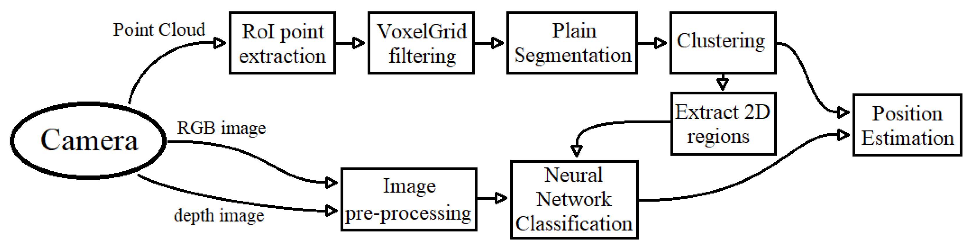
3. Proposed Unified Framework

In this paper, we present a novel unified object classification and position estimation pipeline, which takes advantage of two approaches for object classification. The first is the classical point cloud processing to segment objects from the scene. The second is to use a Convolutional Neural Network (CNN) to classify each object. By finding clusters of points that correspond to objects, we calculate their positions. We then perform object classification using the 2D images of these segments. The proposed framework is summarized in Figure 2 and is described below in detail.

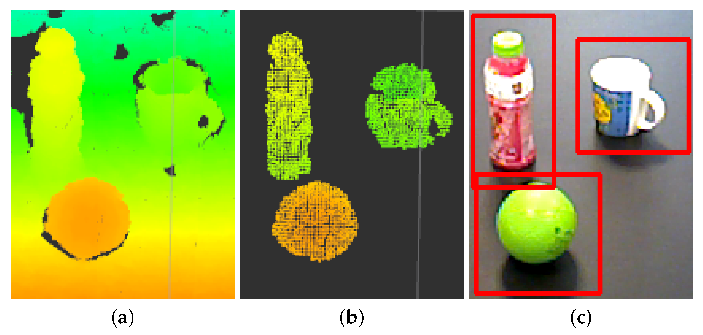
3.1. Object Segmentation Pipeline

For capturing a stream of images, we use an Asus Xtion Pro RGB-D camera. The resolution of the camera 640 × 480 for point cloud produces 307,200 3D points. To reduce the number of points in a point cloud for real-time applications, the PCL provides several methods. Firstly, as shown in Figure 2, we reject all points that are outside the region of interests (RoI) that can be specified as a configuration for the algorithm beforehand. In our experimental robot pick-and-place setup, we have a conveyor belt in the middle of the frame that we set as RoI. To reduce the number of points further we then apply the VoxelGrid filtering algorithm. The VoxelGrid filtering is a downsampling algorithm that reduces the number of points by constructing a 3D voxel array over the input cloud. For each voxel, it computes centroids of points that belong to it. Although computation of the centroid is computationally more expensive than using the center of the voxel, it produces a more accurate representation of the surface. The parameters for the VoxelGrid filter were chosen through trial-and-error such as to reduce the number of points, but at the same time preserve the overall physical shape of a point cloud. The size of the grid is set to 5 mm, which reduced the number of points by five times on average.
The nature of the problem allows us to assume that objects lay on a surface such as a table. As the next stage of the proposed framework, we find the biggest plain in the scene that corresponds to the table using PCL’s implementation of Planar Segmentation. We employ the Random Sample Consensus algorithm (RANSAC) to estimate the points that belong to the table (inliers). RANSAC randomly selects a subset of points and calculates parameters for any given model (model of a plane in our case). These parameters are called a hypothesis. Repeating these steps for a fixed number of iterations the best hypothesis is found. At the end of the loop, the algorithm returns the best hypothesis and all inliers that belong to the best model. By rejecting all the inliers from the scene only the points belonging to objects on the table are left.
Following the pipeline diagram in Figure 2 the remaining points are clustered together to form individual objects. We use the Euclidean Clustering Extraction algorithm to divide points into clusters based on their proximity to each other. The algorithm uses Euclidean distance to determine if points belong to the same cluster. The points are considered to be in the same cluster if they are in the radius r from each other. Radius r is set as a parameter. By changing its value, we can control the size of the clusters. It has to be noted that in our case r has to be larger than the size of the voxel that was used in the Voxel Grid downsampling step. An iterative search of the point in the radius is computationally expensive, thus the PCL uses a KD-tree structure to optimize the algorithm. The modified version constructs a KD-tree from all the input points. The tree is used to find the closest points and check their relative distance. This eliminates the need for checking all points in the set. In the end, the algorithm extracts a set of clusters that contain points for every object on the table.
Due to the nature of RANSAC and noisy information from the camera, there can be present artifacts, i.e., several clusters with a small number of points that have a negative effect on the further steps. We have to filter clusters by their sizes. The minimal size of the cluster can be set as a parameter of the Euclidean Clustering Extraction algorithm. To estimate the object’s position we calculate its centroid. For all points in the cluster, we compute the mean with respect to three coordinates. This represents the relative center of the object. Example segmentation results of the 3 different shape objects are shown in Figure 3.

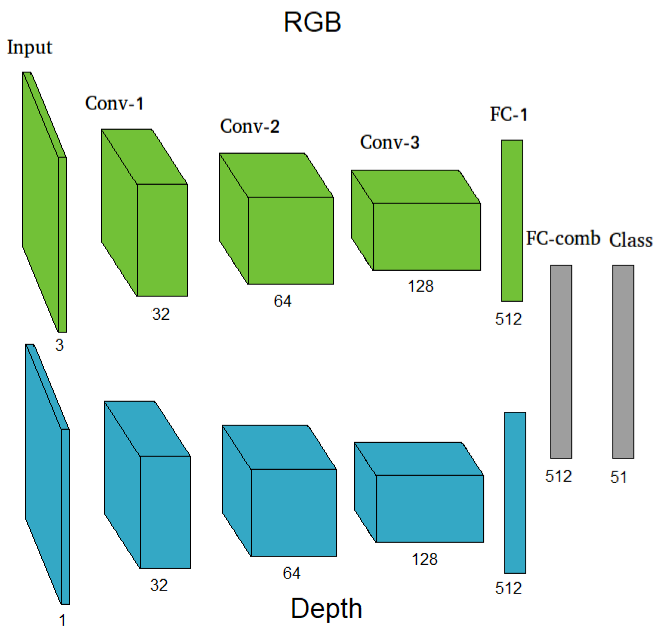
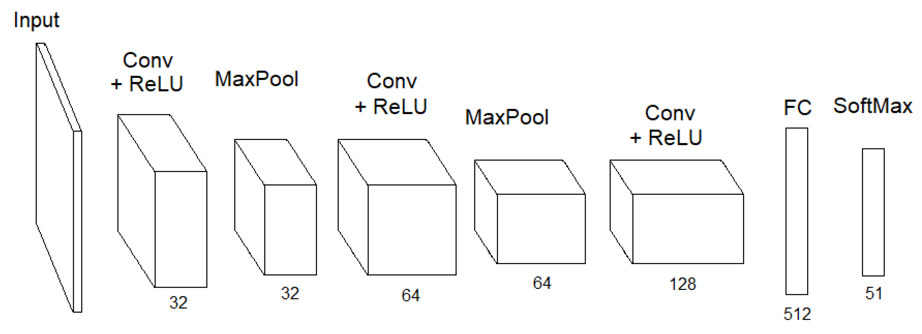
3.2. Object Classification

As indicated in Figure 2, in parallel to the object clustering using 3D point cloud data, the both RBG and depth images acquired from the Asus Xtion Pro RGB-D camera are preprocessed for further object classification with CNN. Using point cloud clusters of the objects described in the previous subsection, it is possible to map 3D points to the 2D RGB and depth images to extract regions that contain objects. These regions are then passed to the neural network for classification.
Object classification is performed using CNN. CNNs are able to learn how to extract features from images effectively for image classification. We use both RBG and depth images acquired from the Asus Xtion Pro RGB-D camera. Using point cloud clusters of the object described in the previous section, it is possible to map 3D points to the 2D RGB and depth images to extract regions that contain objects. These regions are passed to the neural network for classification.
The presented in this paper network was inspired by the work of [16]. The main idea is to reduce the number of parameters in the network, thus decreasing the computational cost for real-time applications. As in the original work, we use two different streams to process RGB and depth information separately and combine two sets of features for classification. In addition, we have trained the network without pre-trained weights. The architecture of our network is presented in Figure 1. The network consists of two streams that perform feature extraction. The first stream takes an RGB image as an input and outputs a feature vector of size 512. The second stream is similar to the first, the only difference is that it takes depth grayscale image as an input and outputs a feature vector of size 512. Two vectors are concatenated to a single 1024 vector and passed through fully connected layers for classification.
The two streams have the same structure except for the first layer. One operates on three-channel input (RGB) and the second on one (depth grayscale). Each stream consists of three convolutional layers, two pooling layers, and one fully connected. The first convolutional layer has 32 filters with a kernel of size 5 by 5 followed by a max-pooling layer with a kernel size of 2 by 2. The second convolutional layer has 64 filters with a kernel of size 5 by 5 followed by a max-pooling layer with a kernel size of 2 by 2. The third convolutional layer has 128 filters with a kernel of size 5 by 5 followed by a fully connected layer with 10,368 neurons and 512 output neurons. After the concatenation of two streams, the output is passed to two fully connected layers. First with 1024 input neurons and 512 output neurons. The second is with 512 input neurons and the number of classes as the number of output neurons followed by a softmax layer. We use ReLU as the activation function in our network.

3.3. Image Pre-Processing

Since our neural network expects input images of size 64 by 64, we apply several image preprocessing steps. First, we rescale the region that was passed from the segmentation step using nearest-neighbor interpolation. It was shown by Eitel et al. [16] that stretched images, produced simple rescaling, negatively affect the performance of the classification. Thus we use the same approach of rescaling the image. We rescale the input image preserving the original ratio to the size of 64 by N or N by 64 depending on the orientation of the image, where N is less than 64. If the shape of the input image is not square we apply the tiling method. A 64 by N or N by 64 image is placed in the middle of a new 64 by 64 image. Then the algorithm repeats border pixels along the longer side for the shorter side axis. The example of the results of such rescaling is shown in Figure 4. This rescaling applied for both RGB and depth segments.
For the depth segment-first, we normalize all values to lie between 0 and 1. We do the same for all three channels of the RGB segment. Then using precalculated mean and standard deviation for the dataset to convert values for all channels of RGB and depth to have a mean of 0 and a standard deviation of 1. Mean and standard deviation values of the RGB are mean_rgb = (0.5446, 0.5227, 0.4804), std_rgb = (0.2094, 0.2139, 0.2612) and for depth mean_depth = 0.5106, std_depth = 0.3380. This flattens the data distribution and helps the neural network converge faster.

3.4. Network Training
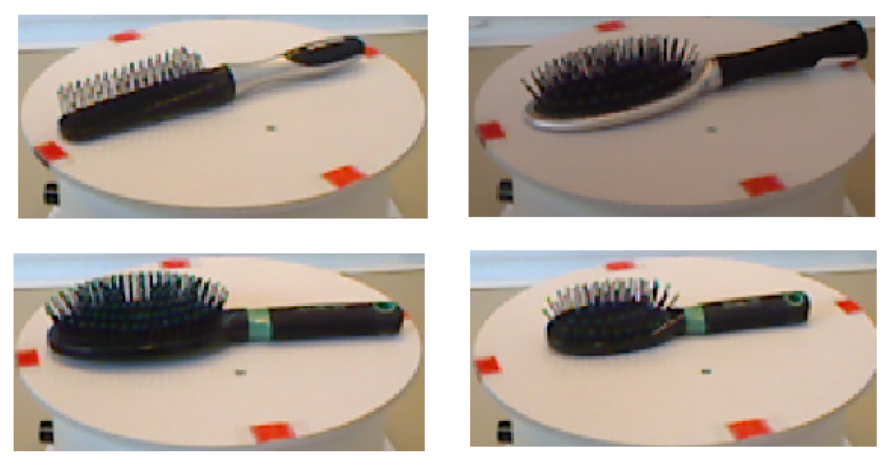
The training was done on a dataset containing both RGB and depth images and image labels in a one-hot encoding vector of size N, where N is the number of classes in the dataset. The training was split into two steps.
The first step is to train two streams (RGB and depth) separately. The initial per stream network is modified by placing a fully connected layer and softmax classifier at the end of the stream. The modified network is shown in Figure 5. The initialization of all parameters of the network (weights and biases) is done randomly. The Stochastic Gradient Descent (SGD) algorithm is used as an optimizer to minimize the loss function.
Let D = {( r 1 , d 1 , t 1 ), ( r 2 , d 2 , t 2 ), …, ( r N , d N , t N )} be the training dataset, where r i denote RGB image, d i is depth image and t i is a one-hot encoded label. Let y I ( r i ) and y D ( d i ) be the output of the last fully connected layer for the RGB and depth streams, respectively, in relation to the inputs r i and d i . As the loss function a negative log-likelihood function is employed:
L ( x i , t i ) = i C log ( s o f t m a x ( y ( x i ) ) , t i ) ,
where x i = r i and y = y I if RGB stream or x i = d i and y = y D if depth stream.
The softmax function is formulated as below:
s o f t m a x ( x i ) = e x i j C e x j ,
where C is the number of classes. By minimizing the negative log-likelihood function (1) the algorithm finds optimal parameters for the network.
After successful training of the two streams, they are combined as follows. In each stream, we replace the last fully connected layer and softmax classifier. Outputs of the remaining layers for both channels are concatenated into a single 1024 dimensional vector and passed to the fusion part of the network (the gray part in Figure 1). The last part of the network is trained using the same algorithm as above.

4. Experiments

4.1. Network Training and Evaluation

The quantitative evaluation of the proposed object classification and position estimation pipeline was done using the Washington RGB-D object dataset [18]. The dataset contained a total of 300 different instances of common household objects divided into 51 separate classes. Each instance was placed on a turntable and captured from three different angles. The images were taken every frame for one complete rotation of the turntable. The total number of RGB-D images in the dataset was 250,000. Objects were organized by classes and instances, which was different from other datasets such as ImageNet. In the Washington RGB-D object dataset, two different instances of the same class represented two different physical objects. This was in contrast to the ImageNet database, where it was impossible to determine if two images were from the same object. The example of different instances of the same category is shown in Figure 6.
The proposed model was evaluated following the procedure described by Lai et al. [18]. RGB and Depth frames are subsampled every fifth frame to get the total 41,877 images for evaluation. The category recognition task in the dataset has 10 different cross-validation splits. Each split has one instance per category (51 instances) for testing and the remaining 249 instances are for training. For every split, the number of RGB-D images for testing is approximately 35,000 and 7000 for testing. The dataset also has an approximated segmentation mask for every image that is used to retrieve the region of interests.
As described above, our pipeline has two streams, three convolutional layers, two max-pooling layers, and two fully connected layers per stream, with two fully connected layers as classifiers at the end. During training, we added several batch normalization layers after every convolutional layer but before their activation. We added a dropout layer with probability 0.2 after the second max-pooling layer and with probability 0.4 after the third convolutional layer in each stream. We also added a batch normalization layer after the first fully connected layer in the fusion part of the network and add a dropout layer afterward with probability 0.5. As a result, we observed that adding batch normalization and dropout layers increased both the learning speed and performance of the network.
The network training was performed in stages. First, we trained RGB and depth streams independently using a batch size of 64. Both streams were trained for 50 epochs using the Stochastic Gradient Descent (SGD) algorithm as optimizer during training with a momentum equal to 0.9 and learning rate set to 0.01, which we changed to 0.001 after 30 epochs. After two streams had been trained we replaced their last fully connected layers with concatenation and proceeded to the next stage, i.e., the training of a full combined network. We used SGD with a momentum of 0.9 and a learning rate of 0.01 as in the previous stages. The network was trained for 50 epochs with the learning rate being reduced to 0.001 after 30 epochs. Two different approaches were compared in the last stage. The first was freezing RGB and depth streams while training the last layers and the second approach was to propagate the gradient throw the entire network. We observed that the stream freezing gives better performance. We also experimented with skipping the first stage and trained everything at once. This also showed a decrease in performance compared to the primary method. To increase the performance we augmented the data set with random horizontal flips during training. The number of epochs and training parameters were chosen from preliminary tests. The training of the single-stream on a PC workstation with Intel Xeon CPU and NVIDIA 1080 Ti GPU graphics card required approximately one hour.

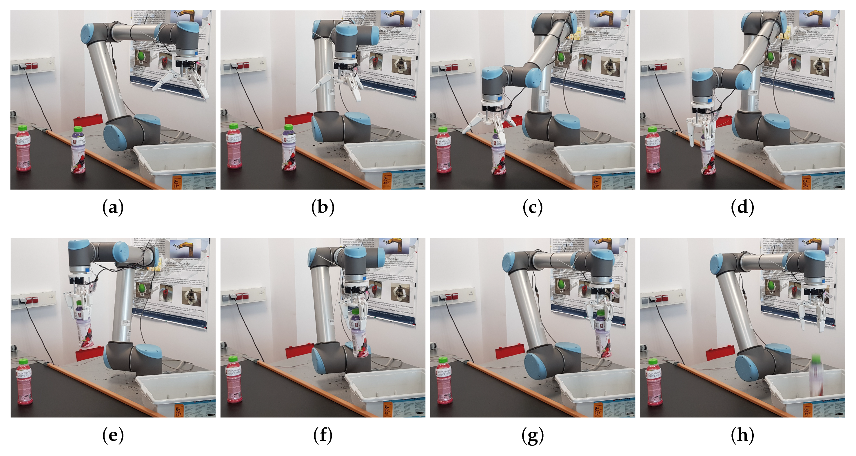
4.2. Experimental Robot-Manipulation Setup

The experimental validation of the presented object classification and position estimation pipeline was conducted on a pick-and-place laboratory setup consisting of a 6-DOF Universal Robots UR10 industrial robot-manipulator controlled in real-time from the Robot Operating System (ROS) programming environment on a control PC by streaming URScript language commands via TCP/IP communication [30,31]. The robot-manipulator was equipped with a custom 3D printed 3-finger adaptive gripper [32] for flexible object picking and was placed near a commercial shop conveyor installation as shown in Figure 9 in Section 5.3. The shop conveyor thus formed a robot working table surface for object grasping, that can be used for implementing static and dynamic (as future work) object picking task scenarios. An Asus Xtion Pro RGB-D sensor was fixed on a holder mounted on the conveyor system (not seen in the figure) for visual and depth data acquisition of the conveyor table scene.
In order to transform points from the RGB-D camera frame to the robot base frame, a corresponding transformation matrix was computed using the following experimental method. The use the RGB-D camera sensor allows to acquire Cartesian coordinates of an arbitrary point is the robot workspace in both the camera frame and the robot base frame. It is done by attaching a marker to the end effector and moving the robot to the desired position. In order to compute the transformation, we define an intermediate frame of reference W. The matrices R T W and C T W , denoting transformation from W to the robot base and camera frames, R and C respectively. The R T W and C T W are computed using the coordinates of four points a , b , c , d I R 3 not lying on the same plane in the respective frames as follows:
v x = a b | | a b | | ; v y = p r o j v x ( a c ) | | p r o j v x ( a c ) | | ; v z = p r o j v x × v y ( a d ) | | p r o j v x × v y ( a d ) | | ;
T = v x v y v z a 0 0 0 1 .
The transformation matrix from the camera to the robot base frame R T C is obtained as follows:
R T C = R T W · C T W 1 .
All system hardware components, data processing, and control algorithms were integrated into ROS. Details of the robot motion planning and control implementations will be shortly reported in the author’s future publication. In order to adapt the developed object classification algorithm to the laboratory setup an additional subset of object images was manually collected. The network was then retrained using transfer learning techniques.

5. Results and Discussion

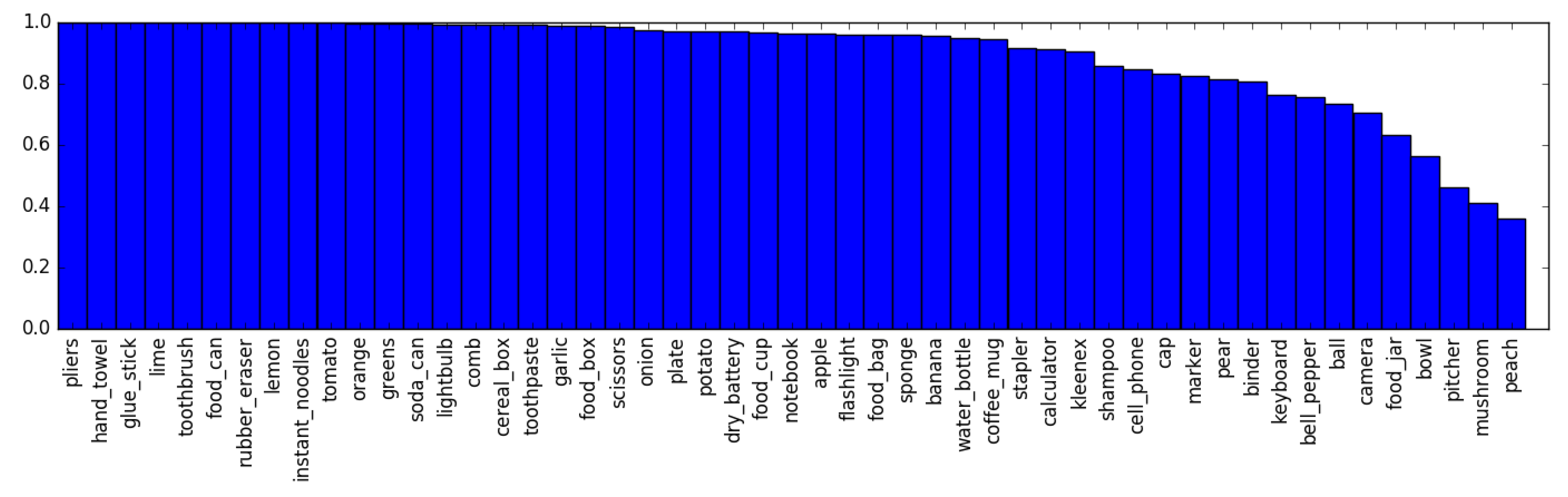
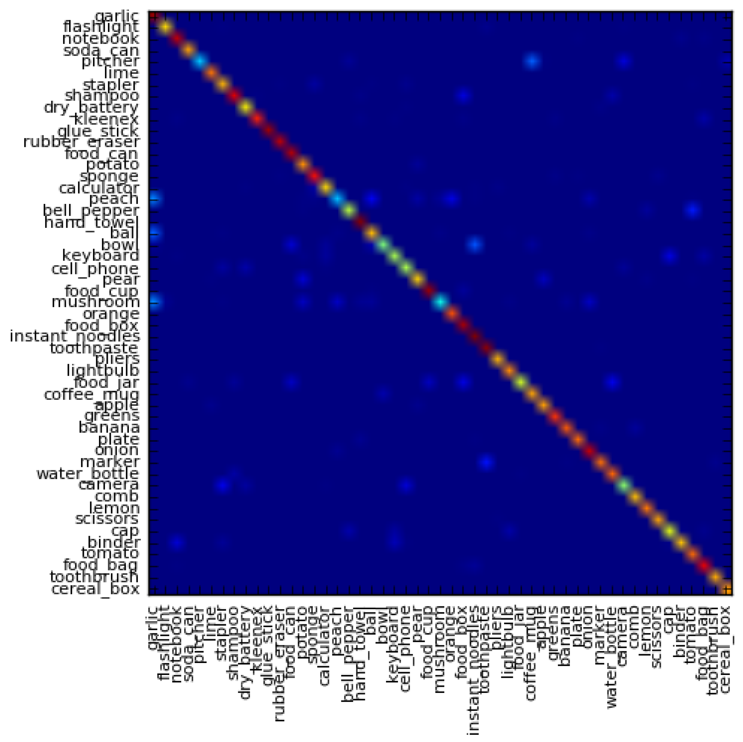
5.1. Classification Accuracy

Table 1 presents a comparison of the classification accuracy results of the proposed framework with several reported state-of-the-art techniques, that previously utilized the same Washington RGB-D dataset [18]. The presented comparison demonstrates that the proposed model is comparable with and in some cases outperforms the other approaches. Specifically, the model obtains 76.3% ± 3.8% classification accuracy for RGB and 76.3% ± 2.1% for depth streams, separately. However, using both RGB and depth streams together, its performance goes up to 86.2% with a standard deviation of 1.3%. This is only 5% less than the most accurate model, VGG3D [29]. Although our framework obtains slightly lower classification scores than VGG3D, CNN Features, and Fus-CNN, it requires much fewer parameters. As a result, it uses less computational time for both inference and training stages, thus, making it more suitable for implementations in real-time systems. Both CNN Features and Fus-CNN are based on the CaffeNet architecture pre-trained on the ImageNet dataset [27]. One stream of the Fus-CNN has five convolutional and two fully connected layers requiring 213,469,216 parameters. In total, the two streams and the last fully connected layers have 460,705,907 parameters. On the contrary, the proposed network reduces the number of convolutional and fully connected layers to three and two, respectively, per stream, yielding a total of 11,684,019 parameters, which is only 2.5% of the original architecture. Comparing the number of parameters of the proposed model to VGG3D, we should note that VGG3D has two streams based on VGGNet-16. The first stream has the same model as VGGNet-16, and the second stream changes the first 2D convolutional layer to a 3D convolutional layer. Moreover, it has an additional stream that is a 3D convolutional network, consisting of two convolutional layers of size 64 by 64 by 64 with a kernel size 3 by 3 by 3 and two fully connected layers. Combined all three streams have more than 230 million parameters, which makes our model size around 5% of VGG3D.
Figure 7 demonstrates the per-call recall of all test splits. We can see that more than half of the classes achieved a recall of more than 95%. The lowest recall of less than 50% showed classes peach, mushroom, and pitcher. This can be explained by the difficulty of the dataset and that these classes have widely different instances or fewer images per category in general. Analyzing the confusion matrix, presented in Figure 8, we can notice that peach class is most often confused with garlic, and to a lesser extent with a ball and orange, a mushroom is confused with garlic, and a pitcher is confused with a coffee mug.

5.2. Computation Performance

The next set of experiments was focused on measuring the execution time of the proposed and the previous frameworks for the inference step. Table 2 shows the average execution time over 1000 iterations along with the number of parameters associated with each method. All models were tested on the same PC workstation with Intel Xeon(R) E5-2620 v4 @ 2.10 GHz × 16 CPU and NVIDIA 1080Ti GPU card. According to the results, the proposed model takes 66.11%, 32.65%, and 28.77% less time than VGG3D, Fus-CNN, and CNN Features, respectively using GPU. When the experiments are conducted on CPU, our model takes 86.91%, 51.12%, and 50.15% less time than VGG3D, Fus-CNN, and CNN Features.
The speedup our model gains is attributed to two main features. One is the decreased number of parameters used by the proposed model and the other is its input size. Namely, the proposed network works with an input of size 64 by 64. In contrast, the CaffeNet and VGG3D both expect an input of size 224 by 224. These results represent the overall speedup gained by our framework despite the slight drop (approximately 5 % ) in the classification performance due to the network simplification. Therefore, the proposed model offers the performance-complexity trade-off between accuracy and speed. Namely, the faster network is less accurate but suitable for real-time applications, while the more accurate architectures are slower and thus not suitable for real-time.

5.3. Experimental Verification

The reported above comparative object classification accuracy and computation performance evaluations of the developed object classification and position estimation pipeline confirmed its potential applicability for designing real-time robotized object pick-and-place systems. This was further experimentally verified through the development of the laboratory robot-manipulation setup described in Section 4.2 and realization of a simplified static object pick-and-place task scenario with the fixed top-down grasping of standing plastic bottle objects as demonstrated in Figure 9. The figure presents a sequence of camera shots in which two 0.5-liter plastic bottle objects were placed on top of the standing still shop conveyer belt. Initially, the robot was in its pre-defined home configuration with an open gripper, as shown in Figure 9a. The system acquires RGB-D images and performs object classification routine using the presented data processing framework. Subsequently, the system determines positions for all identified objects of interest, generates the robot trajectory towards a closest detected object on a scene, and executes the robot motion, as shown in Figure 9b,c. The conversion of the estimated object positions from the camera frame to the robot base frame for the robot motion planning is done using the transformation matrix (4), precalculated using the procedure described in Section 4.2. Subsequently, the object is grasped by the robot gripper fixed in the top-down orientation (Figure 9d) and is then transferred towards a bin, as demonstrated in Figure 9e–g. Once the object is released to the bin, the robot returns to its home position (Figure 9h) and starts a new cycle again. If no objects are detected in the working scene, the robot remains in its home position. The video demonstration of this task accompanies this publication and is also available at the authors’ research lab web-site https://www.alaris.kz and https://youtu.be/Dz-XoVHUdvw.
Multiple test runs resulting in more than 50 picking trials with various distinctive shape objects such as bottle, cup, ball, and others, confirmed the validity of the proposed object classification and position estimation pipeline for the task of repetative real-time detection of selected objects and their picking-and-placing with fixed gripper orientation. The average run-time required to classify and grasp a single object with a robot was approximately 5 s, whereas a complete object pick-and-placing cycle took about 20 s. The relatively slow system performance is explained by the fact that joint velocities of the experimental UR10 robot were limited to 30% from its nominal values due to safety reasons for the pilot testing of the developed object classification and position estimation pipeline. Despite of that, the achieved system performance was, in general, comparable with the reported grasp planning run-times ranging from 0.06 s to 40 s for a number of top-scoring pick-and-place robotic systems, participated in the Amazon Picking Challenge competitions as reported in [12]. In approximately 95% of test trials, the system was able to accurately position the robot over the detected objects of interest in an automatic mode, ensuring stable cyclic execution with time delays. However, due to the use of a simple custom-made 3D printed gripper, the rate of successful object grasps by the robot was slightly lesser and equaled to approximately 80%. Optimization of the system run-time and object grasping performance, that could include relaxing the imposed robot joint velocity constraints with optimizing the robot motion planning algorithm in terms of implementing additional safety features for accounting unexpected presence of human and other obstacles in the robot workspace as well as implementation and testing of various object pose estimation and grasping strategies, was beyond the scope of this work and will the subject of authors’ future research.

6. Conclusions and Future Work

In this paper, we have presented a novel unified framework for object detection/classification and spatial position estimation using a combination of point cloud processing and deep learning techniques. Experimental evaluation of the proposed CNN model including the comparison with the previous works demonstrates its effectiveness and efficiency. Moreover, fewer parameters of the proposed model compared to other multimodal neural networks make our model suitable for real-time applications. In particular, the experiments performed on the Washington RGB-D object dataset [18] show that the proposed framework has 97.5% and 95% fewer parameters compared to the previous state-of-the-art multimodel neural networks Fus-CNN [16], CNN Features [17], VGG3D [29], respectively, with the cost of approximately 5% drop in object classification accuracy. Moreover, experimental results show that the proposed method significantly outperforms previous multimodel neural networks in terms of the inference time. In comparison with the methods presented in [16,17,29], the proposed model takes 66.11%, 32.65%, and 28.77% less time on GPU and 86.91%, 51.12%, and 50.15% less time on CPU respectively. This allowed us to successfully implement the presented framework for real-time object classification and position estimation in the experimental robot pick-in-place setup.
The proposed pipeline is trained using the training subset selected from the Washington RGB-D object dataset. As future work, instead of training the proposed model from scratch, we plan to start the training process from a pre-trained network such as the ones trained on ImageNet [28] or Microsoft COCO [35]. In addition, the network will be modified to overcome the limitation of having all objects located on a plane. Using bounding box object detection techniques, we plan to generalize our framework to detect objects that are not necessarily placed on a single plane.
The experimental robotized pick-and-place system that is presented in this paper is in its early stage of development. Conducted feasibility tests were limited to grasping spherical and vertically standing cylindrical shape objects due to the simple design of the employed robotic gripper in a fixed top-down orientation. Further work will be focused on implementation more sophisticated and realistic operations such as picking occluded objects and placing objects on the shelves. The next step is adopting the approach of the [36,37] in pose estimation and combining it with advanced object grasping while archiving lower system run-times. One of the ideas for further development is a combination of the suction end-effector with the gripper for more reliable object picking. Picking the operation of the moving objects is also planned to be studied.

Author Contributions

Conceptualization, S.S., M.F.D. and A.S.; Data curation, S.S.; Formal analysis, S.S. and M.F.D.; Funding acquisition, A.S.; Investigation, S.S., A.O. and A.S.; Methodology, S.S., M.F.D. and A.S.; Project administration, A.S.; Resources, A.S.; Software, S.S. and A.O.; Supervision, M.F.D. and A.S.; Validation, S.S., A.O. and A.S.; Visualization, S.S.; Writing—original draft, S.S. and A.S.; Writing—review and editing, A.O. and M.F.D. All authors have read and agreed to the published version of the manuscript.

Funding

This research was partially funded under the Nazarbayev University faculty development grant project “Development of an Intelligent Assistive Robot Manipulation System for Improving the Quality of Life of Disabled People in Kazakhstan” (grant no. 090118FD5340) and the Kazakhstan Ministry of Education and Science’s young researchers grant project “Development of an Autonomous Skid-Steering Based Mobile Robot-Manipulation System for Automating Warehouse Operations in Kazakhstan”(Project IRN AP08052091).

Acknowledgments

The authors would like to thank Roman Kruchinin and Anton Kim for their technical support in developing the experimental robot pick-and-place setup and validation experiments.

Conflicts of Interest

The authors declare no conflict of interest.

References

  1. Hossain, D.; Capi, G.; Jindai, M.; Kaneko, S.I. Pick-place of dynamic objects by robot manipulator based on deep learning and easy user interface teaching systems. Ind. Robot. Int. J. 2017, 44, 11–20. [Google Scholar] [CrossRef]
  2. Shi, J.; Koonjul, G.S. Real-Time Grasping for Robotic Bin-Picking and Kitting Applications. IEEE Trans. Autom. Sci. Eng. 2017, 14, 809–819. [Google Scholar] [CrossRef]
  3. Hutchinson, S.; Hager, G.; Corke, P.I. A Tutorial on Visual Servo Control. IEEE Trans. Robot. Autom. 1996, 12, 651–670. [Google Scholar] [CrossRef] [Green Version]
  4. Hager, G.D.; Chang, W.C.; Morse, A.S. Robot Hand-Eye Coordination Based on Stereo Vision. IEEE Control Syst. Mag. 1995, 15, 30–39. [Google Scholar]
  5. Tsai, C.Y.; Wong, C.C.; Yu, C.J.; Liu, C.C.; Liu, T.Y. A Hybrid Switched Reactive-Based Visual Servo Control of 5-DOF Robot Manipulators for Pick-and-Place Tasks. IEEE Syst. J. 2015, 9, 119–130. [Google Scholar] [CrossRef]
  6. Bellandi, P.; Docchio, F.; Sansoni, G. Roboscan: A combined 2D and 3D vision system for improved speed and flexibility in pick-and-place operation. Int. J. Adv. Manuf. Technol. 2013, 69, 1873–1886. [Google Scholar] [CrossRef]
  7. Saudabayev, A.; Khassanov, Y.; Shintemirov, A.; Varol, H.A. An Intelligent Object Manipulation Framework for Industrial Tasks. In Proceedings of the 2013 IEEE International Conference on Mechatronics and Automation, Takamatsu, Japan, 4–7 August 2013; pp. 1708–1713. [Google Scholar]
  8. Rennie, C.; Shome, R.; Bekris, K.E.; De Souza, A.F. A Dataset for Improved RGBD-Based Object Detection and Pose Estimation for Wirehouse Pick-and-Place. IEEE Robot. Autom. Lett. 2016, 1, 1179–1185. [Google Scholar] [CrossRef] [Green Version]
  9. Wurman, P.R.; Romano, J.M. The Amazon Picking Challenge 2015. AI Mag. 2016, 37, 97. [Google Scholar] [CrossRef] [Green Version]
  10. Correll, N.; Bekris, K.E.; Berenson, D.; Brock, O.; Causo, A.; Hauser, K.; Okada, K.; Rodriguez, A.; Romano, J.M.; Wurman, P.R. Analysis and Observations from the First Amazon Picking Challenge. IEEE Trans. Autom. Sci. Eng. 2018, 15, 172–188. [Google Scholar] [CrossRef]
  11. He, R.; Rojas, J.; Guan, Y. A 3D object detection and pose estimation pipeline using RGB-D images. In Proceedings of the 2017 IEEE International Conference on Robotics and Biomimetics (ROBIO), Macau, China, 5–8 December 2017; pp. 1527–1532. [Google Scholar]
  12. Zeng, A.; Song, S.; Yu, K.T.; Donlon, E.; Hogan, F.R.; Bauza, M.; Ma, D.; Taylor, O.; Liu, M.; Romo, E.; et al. Robotic Pick-and-Place of Novel Objects in Clutter with Multi-Affordance Grasping and Cross-Domain Image Matching. In Proceedings of the 2018 IEEE International Conference on Robotics and Automation (ICRA), Brisbane, QLD, Australia, 21–25 May 2018; pp. 3750–3757. [Google Scholar]
  13. Schwarz, M.; Milan, A.; Periyasamy, A.S.; Behnke, S. RGB-D object detection and semantic segmentation for autonomous manipulation in clutter. Int. J. Robot. Res. 2018, 37, 437–451. [Google Scholar] [CrossRef] [Green Version]
  14. Rusu, R.B.; Cousins, S. 3D is Here: Point cloud library (PCL). In Proceedings of the 2011 IEEE International Conference on Robotics and Automation (ICRA), Shanghai, China, 9–13 May 2011. [Google Scholar]
  15. Aldoma, A.; Marton, Z.C.; Tombari, F.; Wohlkinger, W.; Potthast, C.; Zeisl, B.; Rusu, R.B.; Gedikli, S.; Vincze, M. Tutorial: Point Cloud Library: Three-Dimensional Object Recognition and 6 DOF Pose Estimation. IEEE Robot. Autom. Mag. 2012, 19, 80–91. [Google Scholar] [CrossRef]
  16. Eitel, A.; Springenberg, J.T.; Spinello, L.; Riedmiller, M.; Burgard, W. Multimodal Deep Learning for Robust RGB-D Object Recognition. In Proceedings of the 2015 IEEE/RSJ International Conference on Intelligent Robots and Systems (IROS), Hamburg, Germany, 28 September–2 October 2015; pp. 681–687. [Google Scholar]
  17. Schwarz, M.; Schulz, H.; Behnke, S. RGB-D Object Recognition and Pose Estimation Based on Pre-Trained Convolutional Neural Network Features. In Proceedings of the 2015 IEEE International Conference on Robotics and Automation (ICRA), Seattle, WA, USA, 26–30 May 2015; pp. 1329–1335. [Google Scholar]
  18. Lai, K.; Bo, L.; Ren, X.; Fox, D. A Large-Scale Hierarchical Multi-View RGB-D Object Dataset. In Proceedings of the 2011 IEEE International Conference on Robotics and Automation, Shanghai, China, 9–13 May 2011; pp. 1817–1824. [Google Scholar]
  19. Bo, L.; Ren, X.; Fox, D. Depth Kernel Descriptors for Object Recognition. In Proceedings of the 2011 IEEE/RSJ International Conference on Intelligent Robots and Systems, San Francisco, CA, USA, 25–30 September 2011; pp. 821–826. [Google Scholar]
  20. Blum, M.; Springenberg, J.T.; Wülfing, J.; Riedmiller, M. A Learned Feature Descriptor for Object Recognition in RGB-D Data. In Proceedings of the 2012 IEEE International Conference on Robotics and Automation, Saint Paul, MN, USA, 14–18 May 2012; pp. 1298–1303. [Google Scholar]
  21. Bo, L.; Ren, X.; Fox, D. Unsupervised Feature Learning for RGB-D Based Object Recognition. In Experimental Robotics; Springer: Berlin/Heidelberg, Germany, 2013; pp. 387–402. [Google Scholar]
  22. He, K.; Zhang, X.; Ren, S.; Sun, J. Deep Residual Learning for Image Recognition. In Proceedings of the IEEE Conference on Computer Vision and Pattern Recognition, Las Vegas, NV, USA, 27–30 June 2016; pp. 770–778. [Google Scholar]
  23. Simonyan, K.; Zisserman, A. Very Deep Convolutional Networks for Large-Scale Image Recognition. arXiv 2014, arXiv:1409.1556. [Google Scholar]
  24. Krizhevsky, A.; Sutskever, I.; Hinton, G.E. ImageNet Classification with Deep Convolutional Neural Networks. In Advances in Neural Information Processing Systems 25; Curran Associates, Inc.: Dutchess County, NY, USA, 2012; pp. 1097–1105. [Google Scholar]
  25. Szegedy, C.; Liu, W.; Jia, Y.; Sermanet, P.; Reed, S.; Anguelov, D.; Erhan, D.; Vanhoucke, V.; Rabinovich, A. Going Deeper With Convolutions. In Proceedings of the IEEE Conference on Computer Vision and Pattern Recognition, Boston, MA, USA, 7–12 June 2015; pp. 1–9. [Google Scholar]
  26. Gupta, S.; Girshick, R.; Arbeláez, P.; Malik, J. Learning Rich Features From RGB-D Images for Object Detection and Segmentation. In European Conference on Computer Vision; Springer: Cham, Switzerland, 2014; pp. 345–360. [Google Scholar]
  27. Jia, Y.; Shelhamer, E.; Donahue, J.; Karayev, S.; Long, J.; Girshick, R.; Guadarrama, S.; Darrell, T. Caffe: Convolutional Architecture for Fast Feature Embedding. In Proceedings of the 22nd ACM International Conference on Multimedia, Orlando, FL, USA, 3–7 November 2014; pp. 675–678. [Google Scholar]
  28. Russakovsky, O.; Deng, J.; Su, H.; Krause, J.; Satheesh, S.; Ma, S.; Huang, Z.; Karpathy, A.; Khosla, A.; Bernstein, M.; et al. ImageNet Large Scale Visual Recognition Challenge. Int. J. Comput. Vis. 2015, 115, 211–252. [Google Scholar] [CrossRef] [Green Version]
  29. Zia, S.; Yuksel, B.; Yuret, D.; Yemez, Y. RGB-D Object Recognition Using Deep Convolutional Neural Networks. In Proceedings of the IEEE International Conference on Computer Vision, Venice, Italy, 22–29 October 2017; pp. 896–903. [Google Scholar]
  30. Rubagotti, M.; Taunyazov, T.; Omarali, B.; Shintemirov, A. Semi-Autonomous Robot Teleoperation With Obstacle Avoidance via Model Predictive Control. IEEE Robot. Autom. Lett. 2019, 4, 2746–2753. [Google Scholar] [CrossRef]
  31. Andersen, T.T. Optimizing the Universal Robots ROS Driver; Technical University of Denmark, Department of Electrical Engineering: Kongens Lyngby, Denmark, 2015. [Google Scholar]
  32. Telegenov, K.; Tlegenov, Y.; Shintemirov, A. A Low-Cost Open-Source 3-D Printed Three-Finger Gripper Platform for Research and Educational Purposes. IEEE Access 2015, 3, 638–647. [Google Scholar] [CrossRef]
  33. Bo, L.; Lai, K.; Ren, X.; Fox, D. Object Recognition With Hierarchical Kernel Descriptors. In Proceedings of the CVPR 2011, Providence, RI, USA, 20–25 June 2011; pp. 1729–1736. [Google Scholar]
  34. Socher, R.; Huval, B.; Bath, B.; Manning, C.D.; Ng, A.Y. Convolutional-Recursive Deep Learning for 3D Object Classification. In Proceedings of the Advances in Neural Information Processing Systems 25, Stateline, NV, USA, 3–8 December 2012; pp. 656–664. [Google Scholar]
  35. Lin, T.Y.; Maire, M.; Belongie, S.; Hays, J.; Perona, P.; Ramanan, D.; Dollár, P.; Zitnick, C.L. Microsoft COCO: Common Objects in Context. In European Conference on Computer Vision; Springer: Cham, Switzerland, 2014; pp. 740–755. [Google Scholar]
  36. Xu, H.; Chen, G.; Wang, Z.; Sun, L.; Su, F. RGB-D-Based Pose Estimation of Workpieces with Semantic Segmentation and Point Cloud Registration. Sensors 2019, 19, 1873. [Google Scholar] [CrossRef] [Green Version]
  37. Ten Pas, A.; Gualtieri, M.; Saenko, K.; Platt, R. Grasp Pose Detection in Point Clouds. Int. J. Robot. Res. 2017, 36, 1455–1473. [Google Scholar] [CrossRef]
Figure 1. The architecture of the proposed network. The network consists of three parts. Two streams perform feature extraction on RGB and Depth images separately using convolutional layers, shown in green and blue respectively. Features from both streams are combined to perform classification using fully connected layers, shown in gray.
Robotics 09 00063 g001
Figure 2. Diagram of the proposed unified object classification and position estimation pipeline.
Robotics 09 00063 g002
Figure 3. Point cloud object segmentation: (a) original point cloud, (b) downsampled and segmented point cloud, (c) corresponding object segments in a 2D image.
Robotics 09 00063 g003
Figure 4. Example of rescaling. (a,b): original rescaled images with preserved size ratio. (c,d): tiled representation. 0—region is the original image, 1—regions are tiled from borders.
Robotics 09 00063 g004
Figure 5. Modified network for a single stream. The two streams of the network are trained separately in the first step. Partial networks that perform feature extraction are modified by adding another fully connected layer, followed by a softmax layer.
Robotics 09 00063 g005
Figure 6. Example of the Washington RGB-D dataset. Four different instances that belong to the same category: comb.
Robotics 09 00063 g006
Figure 7. Per-class recall on all test splits. The network achieves a recall of more than 95% on more than half of the classes. Classes peach, mushroom, and pitcher have the lowest recall of less than 50%. This can be explained by the difficulty of the dataset. Some classes such as pitcher have only 3 instances that are very different from one another. Some classes have fewer images in general, e.g., mushroom category has 729 compared to 1780 images in ball category.
Robotics 09 00063 g007
Figure 8. The confusion matrix for all test splits shows that the vast majority of categories are classified correctly. Analyzes the confusion matrix shows that peach class is most often confused with garlic, and to a lesser extent with ball and orange, a mushroom is confused with garlic, and a pitcher is confused with a coffee mug.
Robotics 09 00063 g008
Figure 9. Video frames at eight different time instants during the autonomous bottle object picking-and-placing test performed by the experimental robot setup.
Robotics 09 00063 g009
Table 1. Accuracy comparison of the proposed CNN with other reports on the Washington RGB-D object dataset for a category recognition task (in percent).
MethodRGBDepthRGB-D
Nonlinear SVM [18]74.5 ± 3.164.7 ± 2.283.9 ± 3.5
HKDES [33]76.1 ± 2.275.7 ± 2.684.1 ± 2.2
Kernel Desc. [19]77.7 ± 1.978.8 ± 2.786.2 ± 2.1
CKM Desc. [20]N/AN/A86.4 ± 2.3
CNN-RNN [34]80.8 ± 4.278.9 ± 3.886.8 ± 3.3
CNN Features [17]83.1 ± 2.0N/A89.4 ± 1.3
Fus-CNN (jet) [16]84.1 ± 2.783.8 ± 2.791.3 ± 1.4
VGG3D [29]88.96 ± 2.178.43 ± 2.491.84 ± 0.89
Proposed model76.3 ± 3.876.3 ± 2.186.2 ± 1.3
Table 2. Average execution time over 1000 iterations in ms of the proposed and other CNN models running on a PC workstation with Intel Xeon(R) E5-2620 v4 @ 2.10 GHz × 16 CPU and NVIDIA 1080Ti GPU card.
MethodOn GPU, msOn CPU, msParameters
VGG3D [29]4.491812.918 230 × 10 6
Fus-CNN [16]2.260217.595 460.7 × 10 6
CNN Features [17]2.137213.389 460.7 × 10 6
Proposed model1.522106.369 11.7 × 10 6

