Cloud-Edge Suppression for Visual Outdoor Navigation

Computer Engineering Group, Faculty of Technology, Bielefeld University, D-33615 Bielefeld, Germany
*
Author to whom correspondence should be addressed.
Robotics 2017, 6(4), 38; https://doi.org/10.3390/robotics6040038
Submission received: 25 September 2017
/
Revised: 22 November 2017
/
Accepted: 27 November 2017
/
Published: 3 December 2017
Abstract
:Outdoor environments pose multiple challenges for the visual navigation of robots, like changing illumination conditions, seasonal changes, dynamic environments and non-planar terrain. Illumination changes are mostly caused by the movement of the Sun and by changing cloud cover. Moving clouds themselves also are a dynamic aspect of a visual scene. For visual homing algorithms, which compute the direction to a previously visited place by comparing the current view with a snapshot taken at that place, in particular, the changing cloud cover poses a problem, since cloud movements do not correspond to movements of the camera and thus constitute misleading information. We propose an edge-filtering method operating on linearly-transformed RGB channels, which reliably detects edges in the ground region of the image while suppressing edges in the sky region. To fulfill this criterion, the factors for the linear transformation of the RGB channels are optimized systematically concerning this special requirement. Furthermore, we test the proposed linear transformation on an existing visual homing algorithm (MinWarping) and show that the performance of the visual homing method is significantly improved compared to the use of edge-filtering methods on alternative color information.
1. Introduction
Navigation is a fundamental task for outdoor robots, as it allows the robot to operate autonomously in an unknown environment. The applications for autonomous outdoor robots range from consumer-oriented products like lawn mowers to search-and-rescue robots [1,2]. Advanced sensors, e.g., differential GPS and LIDAR, exist to allow autonomous navigation of robots. Differential GPS provides the robot with adequate measurements, but it is expensive and not applicable in all environments, as for example in urban canyons [3]. LIDAR devices contain moving mechanical parts, have a limited life-time and pose technological challenges in production. With these limitations in mind, cameras are attractive sensors, as they are low-cost products without moving parts and can be used for several different tasks, such as navigation, terrain classification [4,5] and obstacle avoidance. Thus, visual navigation based solely on camera information is a reasonable choice for consumer-oriented products. Here, we use a fisheye lens to capture panoramic images. Panoramic images allow for separation of rotational and translational motion components [6] and simplify visual navigation methods as the visible image content is independent of the robot’s orientation.
One approach to visual navigation is local visual homing, which can be used for navigation based on topological maps. Local visual homing compares the current view with a snapshot taken at a previously visited place and computes a home direction pointing to the place at which the snapshot was taken. Visual homing algorithms can be divided mainly into two branches: holistic and feature-based methods [7,8]. Feature-based methods extract salient features in the environment and match these features between images [9,10,11], whereas holistic methods operate on the whole image [7,12,13]. Recently, methods were proposed that combine holistic and feature-based approaches [14]; a comparison of both branches can be found in [15].
All visual homing methods have to cope with misleading information in the sky, resulting from moving clouds. Edge filtering is an important preprocessing step for visual homing to improve the illumination invariance [16,17]. Therefore, we propose a linear transformation of RGB input as a preprocessing step for edge filtering, which preserves edges in the ground region of the image while suppressing edges in the sky. Especially holistic visual homing methods, which use all pixels of an image, are affected by these sky edges. Our experiments show that a transformation of the color information before the edge-filtering step improves the homing performance for the holistic MinWarping visual homing method. However, also feature-based approaches may benefit from the proposed method by suppressing visual features in the sky. Even though features detected in the sky portion will ultimately be rejected by the outlier elimination, a decreased outlier portion decreases the computational effort. According to [18], an outlier rejection like RANSAC (random sample consensus) can often find the right solution even for a high amount of outliers. However, the number of required samples increases exponentially, and the increase in the computational cost is substantial. In particular, the proposed method could be beneficial for all visual homing methods which operate on color images, especially edge-filtered color images, in outdoor environments.
In this paper, we focus on the use of warping, more precisely the refined MinWarping [7,16], a holistic visual homing method that has successfully been applied in indoor environments [19,20]. As many holistic methods, MinWarping considers all pixels of an image by computing a pixel-wise distance measure and is therefore affected by scene changes not caused by camera movements. In practical applications, a human or animal moving through the image only affects a relatively small part of the image, but moving clouds can affect a substantial portion of the image. In this paper, we focus on this issue by proposing an edge-detection method, which implicitly suppresses misleading information in the sky region caused by clouds by applying an optimized linear transformation on the RGB input. A straightforward exclusion of the sky region by restricting the vertical opening angle for the camera images is not feasible, because the area of the image that is covered by sky strongly depends on the environment.
Previous studies [16] showed that MinWarping performs best on edge-filtered images with respect to illumination tolerance; however, standard edge detection algorithms lead to prominent edges in the sky caused by clouds. The proposed method is illustrated in Figure 1: As can be seen, the Prewitt filter applied to standard RGB channels followed by a maximum operation produces an edge image with distinct edges in the sky, whereby the proposed method (denoted as ) leads to an edge-filtered image in which the edges in the sky are substantially fainter.
The paper is organized as follows: In Section 2, we give an overview of the state of the art of algorithms for edge suppression in the sky region of an image. We proceed in Section 3 by describing the proposed linear transformation for RGB input channels and the image preprocessing pipeline used for all the performed experiments. This is followed by the description of the analysis methods in Section 4, which include the definition of application-oriented performance criteria in Section 4.1, a concise recapitulation of the MinWarping method used for homing experiments throughout this paper in Section 4.2 and a short description of alternative methods in Section 4.3. Section 5 describes the experimental setup and the databases. The results are presented and discussed in Section 6. The paper is completed by a short conclusion in Section 7 and an outlook toward future works (Section 8).
2. Related Work: Edge Suppression
In this section, we review approaches that provide edge suppression in the sky, while preserving edges in the ground region of an image. The aim is to compute reliable edges for visual navigation in outdoor environments. In this context, edges resulting from moving clouds in the sky represent misleading information and are therefore considered as unreliable.
In the last few decades, comprehensive research on color edge detection has been performed. Most of the proposed methods for edge detection in color images pursue the detection of all salient edges in an image. Edge-detecting procedures operating on color images can be divided into two groups: monochromatic-based and vector-valued techniques. Monochromatic-based techniques use classical edge-detection techniques on each color channel separately and then combine the individual results in a specific manner [21,22,23,24,25,26,27,28,29]. On the contrary, vector-valued techniques regard the color information as vectors [30,31,32,33,34,35,36]. Furthermore, biologically-inspired edge-detection techniques exist (e.g., [37]), which are based on the concept of color-opponency and use color differences as the basis for edge detection. None of these methods distinguish between edges in the sky and edges in the ground region of an image and are therefore not relevant for our problem formulation; for further reading, we refer to available reviews [38,39,40,41]. Moreover, the particular type of edge filter is not relevant for our application, as MinWarping uses detected edges in a strongly low-pass-filtered image, and the detected edges are not needed for demanding subsequent steps like object segmentation.
Another approach to distinguish sky from ground regions is to use additional sensors to capture images with a larger optical spectrum. For example, UV light itself or in combination with green can be used to reliably separate sky from ground in images [42,43,44,45]. Infrared light also allows the separation of sky and ground, as [46] show by solving an energy maximization problem. However, these approaches need additional sensors and are therefore not suitable for applications relying on standard color cameras. In [47], an algorithm based on energy function optimization is proposed, which separates sky and ground by only using a standard color camera. This algorithm successfully separates the ground and sky region in the presence of relatively simple and smooth sky region borders. For complex sky borders that are present in natural environments, the authors mention that only a rough outline of the border can be computed. The work in [48] proposes a segmentation of ground and sky regions based solely on RGB input. They perform a linear transform on the RGB input to enhance the sky/ground contrast. On the contrast-enhanced channel, a thresholding operation separates sky and ground. This method is used for visual navigation in [49,50] as a preprocessing step to blacken the sky region before the images are compared. Note that all these approaches require an additional computation step, as the sky and ground regions have to be separated before an edge-filtering method can be applied on the thresholded image.
Other approaches focus on classifying detected edges by their physical properties. The work in [38] describes a method to classify edges, based on their physical origin, into the following classes: object edges, reflectance edges, shadow edges, specular edges and occlusion edges. The classification is based on the dichromatic reflection model [51]; therefore, certain knowledge of the material properties is required to apply this method. The work in [52] also classifies edges based on their physical properties. They propose a parameter-free edge classifier for the following classes: shadow-geometry, highlight edges and material edges. In both approaches, the proposed classification is not suitable for edges caused by clouds, which cannot be regarded as solid objects, as they do not fit into any of these classes.
More sophisticated approaches focus on boundary detection instead of classical edge detection. According to [53], a boundary is a contour that represents a change in pixel ownership from one object or surface to another, whereas an edge corresponds to an abrupt change in low-level features. An overview of boundary detection algorithms is presented by [54]. The approach of [53] combines different cues of local image measurements to learn the occurrence of boundaries within a supervised learning model. The ground truth for evaluating classified edges are human-labeled color images. The work in [55] performs boundary detection based on the method by [53] and adds image segmentation as a further step. Moreover, [56] propose to use Laplacian eigenvectors to extract globally-significant boundaries from color images. None of these approaches is relevant for our research, as they do not allow the discrimination of edges in sky or ground regions. Furthermore, in the ground region, structure inside of objects might hold important information for visual homing methods (e.g., MinWarping) and, thus, should not be suppressed.
We propose an edge-detection method based on a linear transformation of the RGB channels for detecting reliable edges in the ground region of the image while simultaneously suppressing edges in the sky region. Our approach is similar to the linear transformation by [48] described above, but we optimize the factors of the linear transformation regarding the ratio between edge responses in the sky region and edge responses in the ground region of an image. The analysis allows us to select one specific set of factors that show the desired properties: edges in the ground region are reliably detected, while edges in the sky regions are suppressed. We perform the edge filtering on the transformed RGB input without a thresholding step to segment the sky and ground regions. We show that this approach markedly improves the performance of a subsequent homing step using MinWarping.
3. Suggested Cloud-Edge Suppression Method
In this section, we describe the proposed cloud-edge suppression method including the image preprocessing pipeline, which provides the input for the linear transformation on RGB channels.
3.1. Image Preprocessing
For the proposed method, the raw camera images are passed through a preprocessing pipeline, which is sketched in Figure 2. The original images have a size of 1280 × 1024 pixels and are captured with seven or eight different exposure times (0.12 ms, 0.25 ms, 0.5 ms, 1.0 ms, 2.0 ms, 4.0 ms, 8.0 ms, 16 ms (16 ms is only used for the databases (a)–(c), and (e))). First, the low dynamic range images are combined into a high dynamic range image using the HDR procedure described in [57]. We use the modified version from [43] and compute the HDR images for each RGB channel separately. This step is included to avoid problems with over- and under-exposure of the images. The resulting HDR image is low-pass filtered by applying a standard two-dimensional Gaussian filter:
The Gaussian filtered images are then used as the input of an edge-detection method, which is implemented as a simple Prewitt operator. For comparison, we tested different inputs for the edge-filtering step: the proposed linear transformation on RGB channels (described in detail in Section 3.2), all RGB channels independently followed by a combination of the edge-filtered channels by a maximum operation and the linear transformation described in [48].
Further preprocessing steps are applied to use the images for a visual homing method (here: MinWarping). The grey-scale edge-filtered image is aligned using the measurements from the attached IMU, such that the optical axis of the camera corresponds to the gravity vector. In the next step, the rotated image is mapped to a rectangular panoramic view using the mapping from the OCamCalib toolbox [58]. Finally, the image is subsampled such that the final image has a size of 288 × 72 pixels.
3.2. Linear Transformation on RGB Channels
To achieve our goal of detecting reliable edges in the ground region of the image while suppressing edges in the sky region, we propose a linear transformation of the RGB input as a preprocessing step of a simple edge detection which is similar to the approach in [48]. The approaches differ in the goal of the optimization: in [48], the authors search for a good parameter combination to segment the sky from the ground region, whereas we try to maximize the so-called sky-to-ground ratio, which is described in detail in Section 4.1. We show that the sky-to-ground ratio is a suitable criterion as it results in a good homing performance using MinWarping.
As a simple edge-detection method, we use the Prewitt kernels as defined in Equation (2) to compute image gradients and combine the gradients to obtain the edge magnitude (see, e.g., [59]).
The linear transformation of the RGB input is described as:
where , and denote the weights for the R, G and B channels, respectively. The range for is [0,1], and and are in [−1,1]. Without loss of generality, all sets of weights have to fulfill the condition .
This parameterization spans a parameter space formed by the surface of a hemisphere with radius one. In Figure 3a, this parameter space is sketched. The angle controls the weight for the red channel in the linear combination; results in in the linear combination; and results in . The choice of the angle controls the ratio of the green and blue channels. Note that the other hemisphere is a center-symmetrical copy, as only the edge sign changes (which is eliminated by the edge magnitude computation using the Prewitt operator).
In Figure 3b, the selection of the parameter combinations and the visualization step is sketched. We sampled the parameter space in steps in [−1,1] for and . For each square of which the center lies within the circle, the corresponding linear factors are computed by transforming the square coordinates to spherical coordinates using a linear relationship between d and :
The corresponding linear factors are computed by transforming the point on the hemisphere back to Cartesian coordinates:
To include parameter combinations with , we set for all cropped blocks on the circumference.
4. Performance Analysis
As previously mentioned, visual navigation in outdoor environments requires reliable edges in the ground region of the image, while edges in the sky region should be suppressed. Therefore, we analyze the response of a standard Prewitt filter on linearly-transformed RGB channels and define suitable criteria. Furthermore, we describe the performance criterion used to analyze the results of subsequent homing experiments, as well as the visual homing method MinWarping applied in these experiments. Moreover, three alternative methods are introduced, which are used for comparison in homing experiments.
4.1. Analysis of Edge Response: Sky-To-Ground Ratio and Edge Intensity
For each image, we manually created a mask using an image editing software, which represents the ground truth for the sky and ground regions in the image. These masks are only used for the analysis of the sky-to-ground ratio and for tests with MinWarping to show the effect of sky information on the homing performance. An example of an input color image, a corresponding edge response and the associated mask image is shown in Figure 4.
We search for a linear transformation of RGB channels that maximizes the edge response in the ground region, while minimizing the edge response in the sky region. Crucial are the factors of the linear transformation, not the edge filtering method, as MinWarping operates on first Gaussian-filtered and then edge-filtered input. Thus, only a rough form of the edges is used, and the difference of specific edge-filtering approaches is not relevant. As a consequence, we decided to use the simple Prewitt filter for the edge-filtering step.
To find the best linear transformation of RGB channels to the RGB weighted channel (called in the following), the parameter space described in Section 3.2 is sampled on a grid basis. We then analyze the edge responses on the transformed channels in two regions of the image: ground region and sky region (see Figure 4c). As a performance measure, we define the following sky-to-ground ratio criterion (SGR):
where and are the total edge response within the ground and sky region, respectively, and is the total edge response throughout all regions in one image i. The total edge response is calculated by summing up all pixel values in the edge-filtered image inside the considered region.
A potential drawback of the SGR criterion is that the criterion may yield a high value when the overall edge response is weak. In this case, no meaningful conclusion about the ratio between ground and sky edges can be drawn. An overall weak response of the edge detection filter goes along with a weak response in the ground region in the image. This conflicts with our aim to detect reliable edges in the ground region. To overcome this drawback, we include a further criterion, which measures the edge intensity within the ground region of the image. This so-called edge intensity criterion (EI) is computed as:
where is the summed edge response in the ground region of one image. The criterion is computed for each image separately, averaged over all images i. The resulting values are then normalized to a maximal value of one by dividing through the maximal value reached throughout the parameter combinations .
4.2. Analysis of Homing Performance: MinWarping
To show the applicability of the previously described linear transformation and the defined criteria, we analyze them in realistic visual homing experiments. We selected MinWarping [7] as a holistic visual homing method, which was tested exhaustively in indoor environments, and use the SIMD -implementation (Single Instruction Multiple Data) as published in [60] (available from www.ti.uni-bielefeld.de/html/people/moeller/tsimd_warpingsimd.html). The implementation was extended to allow for ignoring invalid pixel values in the images, which occur due to the alignment of the images to the gravity vector. In image columns, invalid regions only exist at the bottom; thus, we use an adapted version of the normalized sum of absolute differences (NSAD) to calculate the difference between two image columns x and y:
where k and l are the highest indices of the valid pixels in the columns x and y, respectively. The row index is zero at the upper image border. As we use a fisheye lens, only the index of the highest valid pixels are needed; for other omni-directional camera setups, the index of the lowest valid pixels might also be needed. In the denominator in Equation (11), we can omit the computation of the absolute values of the terms, in contrast to the standard NSAD measure, because the applied edge-detection methods only compute positive responses.
The parameters for MinWarping are set according to Table 1 and remain constant through all tests. For the computation of the column-wise NSAD measure, we ignore the topmost image rows in the unfolded images and thus prevent the use of strongly distorted image regions. The ignored rows correspond to 20° of the elevation angle as listed in Table 1.
As a performance criterion, the average angular error (AAE) between the real homing angle and the computed homing angle is used. The AAE is calculated for each database separately and additionally averaged over all databases. In Figure 5, the design of the experiments is illustrated. One image of the database is selected as the snapshot, and all other images are used as current views. Then, home vectors are computed from each current view to the selected snapshot. This is repeated for all available snapshots.
4.3. Alternative Methods
To compare our proposed method with alternative methods, we selected the following three methods:
- : Prewitt filter applied on each RGB channel separately and afterwards combined by a maximum operation.
- : Prewitt filter on the contrast-enhanced channel proposed in [48] as . This can be normalized and inverted to fit into our parameter space and results in . The nearest parameter combination to in our sampled space is indicated by a marker “x” in the plots.
- : Prewitt filter as in , but followed by a sky blackening similar to the approach in [48,49], but using the widespread thresholding method proposed in [61]. The adaptive thresholding was customized to handle panoramic images by weighting the pixels within a column to reduce errors from contortions (the details are given in the Appendix).
5. Experimental Setup
For image acquisition, a CMOS color sensor (IDS: UI-1240LE-C-HQ) with an extreme wide-angle fisheye lens (Lensagon: CSF5M1414) was used. The fisheye lens has a viewing angle of 182°. Attached to the camera is an inertial measurement unit (IMU) (Xsens: MTi-30 AHRS).
For evaluation of the experiments, the test fields were surrounded by four colored landmarks, which were manually marked in the resulting images to extract their positional information. For each image, additional orientational data provided by an IMU were used to compute a three-dimensional ground-truth position of the image, which is especially important for databases collected on uneven terrain, as is the case in three of the six databases. The colored landmarks are barely visible in the panoramic images and probably have no effect on MinWarping.
Databases
The basis for our evaluations is a total set of 464 images, with multiple exposure times for each image. For the databases (a)–(c) and (e), we use eight different exposure times, and for the databases (d) and (f), we use seven exposure times. The images are organized into six databases, which can be categorized into three classes: grid databases (a)–(d), daytime database (e) and route database (f). Figure 6 shows the environments where the databases were collected, and Figure 7 shows one panoramic example HDR image for each database. Additionally, we give a short description of the databases:
- (a)
- Finnbahn: We captured 36 images on a grid of 5 × 5 m, with approximately a 1-m distance between the images. The environment is characterized by surrounding trees and bushes, as well as distant buildings. Throughout the image-capturing process, the cloud cover changed only slightly and remained heavily clouded. The maximal difference in height over the grid is 0.6 m.
- (b)
- Garden 1: We acquired this database with 48 images in a garden on a grid of 7 × 5 m in approximately 1-m steps. Here, small buildings are visible in most of the images, as well as trees and bushes. The main challenge of this database is the occurrence of occlusions and overhanging bushes, as well as the rapidly-moving clouds. The maximal difference in height over the grid is 0.6 m.
- (c)
- Garden 2: We captured 56 images on a 7 × 6 m grid in a garden in approximately 1-m steps. The maximal difference in height is 0.25 m. The main differences to the Finnbahn database are the existence of overhanging trees and a significant change in the cloud cover. Moreover, objects like a compost heap and a shed are partially very close to the camera and dominate some images.
- (d)
- University: On a street next to the Bielefeld University main building, we collected a total of 84 images covering a grid of approximately 29 × 4.75 m with 1.44-m steps along the long side and 1.58-m steps along the narrow side. The changes in roll and pitch angles between the images are small, and no overhanging objects occur. Furthermore, this database was collected under an almost cloudless sky. Dominant in the images is the nearby university building and a line of almost indistinguishable trees in the distance. All images are captured approximately on a plane.
- (e)
- Balcony: This dataset consists of 128 images captured throughout one day during a time span of approximately ten hours in five-minute intervals at the same camera position. The cloud cover changes permanently throughout the image capturing process. These images are only used to evaluate the sky-to-ground ratio of the edge-filtered images (see Section 4.1).
- (f)
- Route: For this database, we collected 109 images in approximately 5-m intervals along a route near the main building of Bielefeld University. As for the balcony setup, no ground truth is available for this database. About half of the images are captured under a completely overcast sky with barely visible changes in the cloud cover. The other half of the images are captured under a slightly overcast sky, which changes only slowly. The images are only used to evaluate the ground-to-sky ratio described in Section 4.1.
6. Results and Discussion
On the basis of the described databases, we performed systematic tests. These tests focus on three aspects: (1) analysis of the SGR criterion across the whole parameter space, (2) investigation of the relationship between the SGR criterion and the MinWarping performance and (3) comparison of the proposed method to alternative methods.
6.1. Analysis of the Sky-To-Ground Ratio
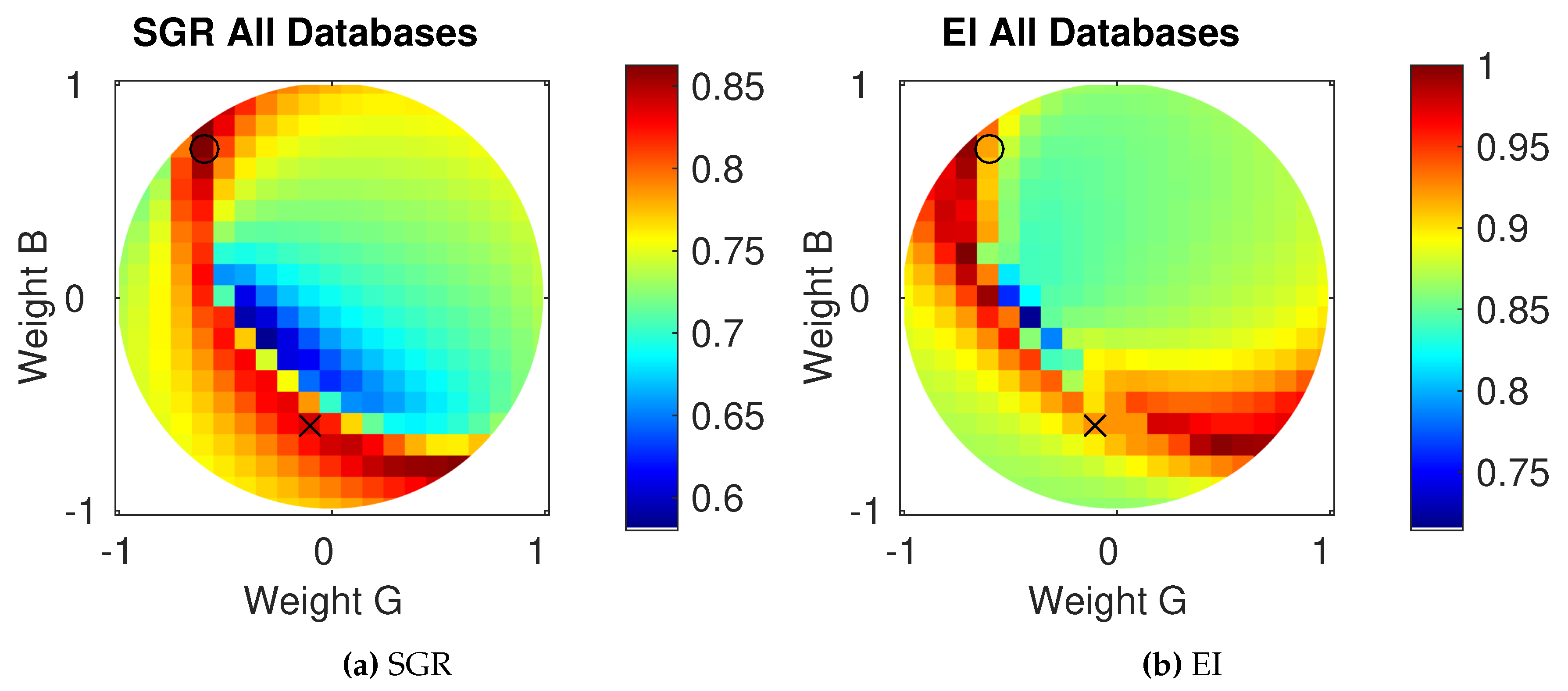
In this section, we describe and discuss the results of different linear combinations regarding the SGR criterion (see Section 4.1) based on the databases described in Section 5.1. In Figure 8a, the SGR criterion is shown for the chosen gridded samples of linear factors averaged over all 464 images (Equation (8)). The diagram reveals a maximum of the SGR criterion near the circumference, which corresponds to a small weight for the red channel. The optimal weights are for the red channel, for the green channel and for the blue channel (marked by a ⚬ in the figures).
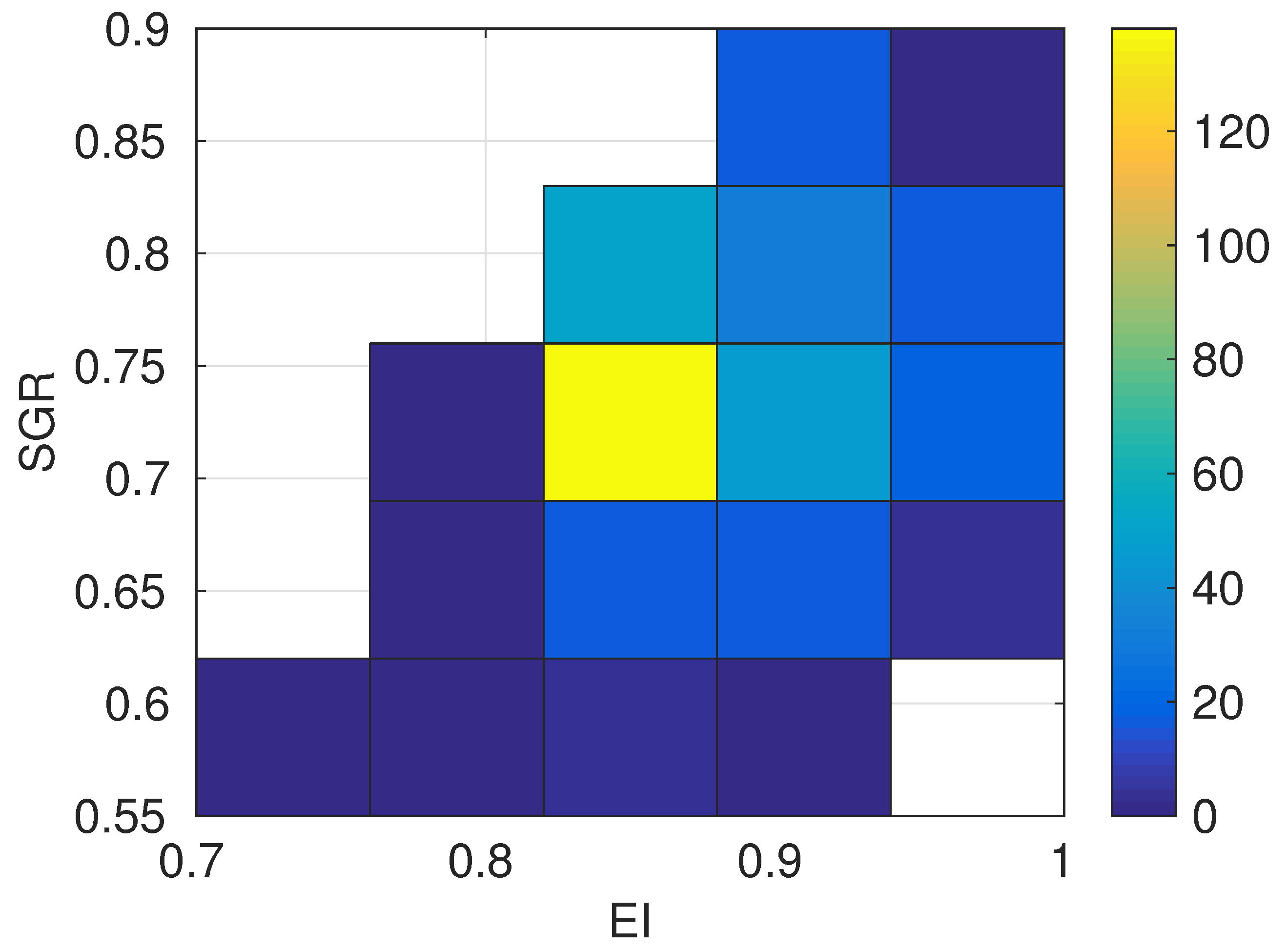
Additionally, in Figure 8b, the EI-criterion is plotted for the sampled linear combinations. Based on this plot, the above choice of , and is justified by the fact that the EI-criterion indicates a strong edge response in the related region. Altogether, high SGR values do not co-occur with low EI values, but low values of EI coincide with low values of SGR. This is additionally illustrated in Figure 9 in the form of a bivariate histogram of SGR and EI values. This diagram is based on the SGR and EI values for the sampled parameter combinations averaged over all databases. Most common is the co-occurrence of average EI values with average SGR values. Important is the upper left part, which shows that high SGR values do not co-occur with low EI values. Moreover, the highest SGR values co-occur with average or high EI values.
Based on these criteria, we propose the following linear transformation:
6.2. Analysis of Homing Performance
The previous section showed that a pronounced maximum of the SGR criterion can be found in the parameter space. Here, we describe and discuss the results in an application-oriented context using the MinWarping method and relate the SGR criterion with the MinWarping performance (for MinWarping details, see Section 4.2).
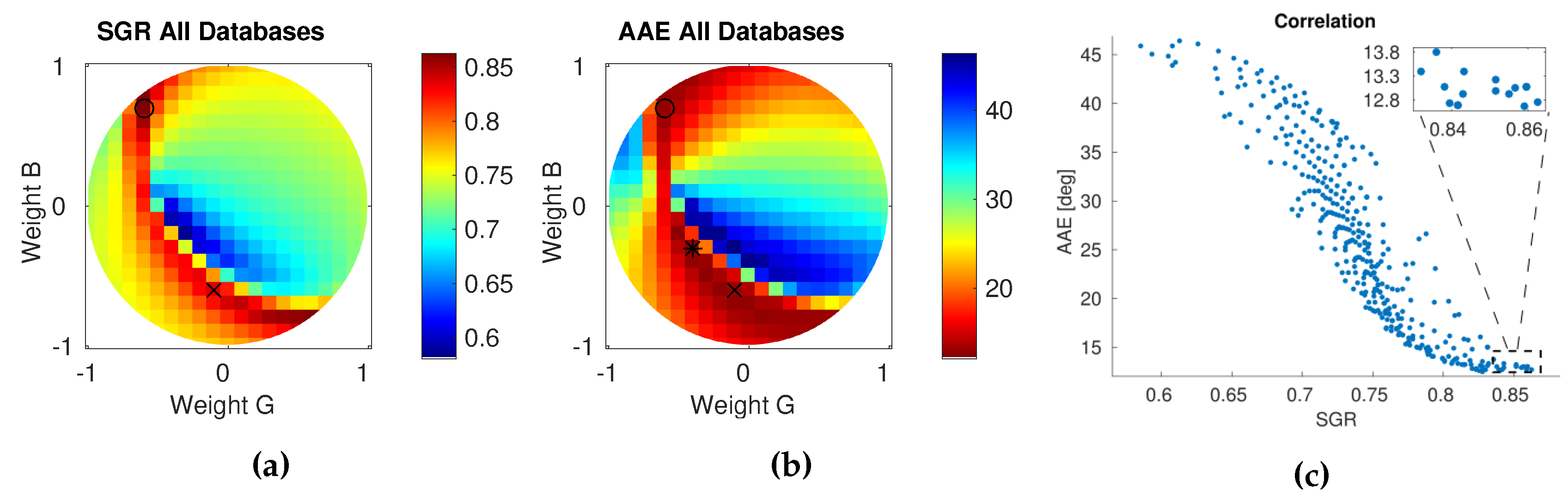
To investigate this relationship, we performed homing tests on the same sampled linear combinations as used for the computation of the SGR criterion. The results are shown in Figure 10 in the center. On the left, the corresponding plot of the SGR values is shown again for better comparison. Note that the color map for the AAE is flipped, such that red colors indicate good results (low angular errors). The plots show a strong correlation between the SGR criterion and the MinWarping performance, which is underlined by the scatter plot shown in Figure 10c on the right. This plot suggests a strong, non-linear correlation between the two variables. We validate this presumption by using Spearman’s correlation coefficient taking into account the non-linearity of the relationship. The Spearman’s correlation test shows a strong, negative monotonic correlation between AAE and SGR (, with ). This corroborates the assumption that the SGR criterion is a good criterion for the search of a linear transformation that improves the performance of homing in outdoor environments. High SGR values and low AAE results could also occur if the sky regions in the images are small and thus barely influence the homing performance. In Section 6.3, we address this issue by using masks to eliminate the sky region and show that the sky region has a strong influence on the homing performance. According to Figure 10, the factors of the linear transformation have a strong effect on the MinWarping performance, resulting in AAE values reaching from approximately 12° for the best up to 47° for unsuitable factors.
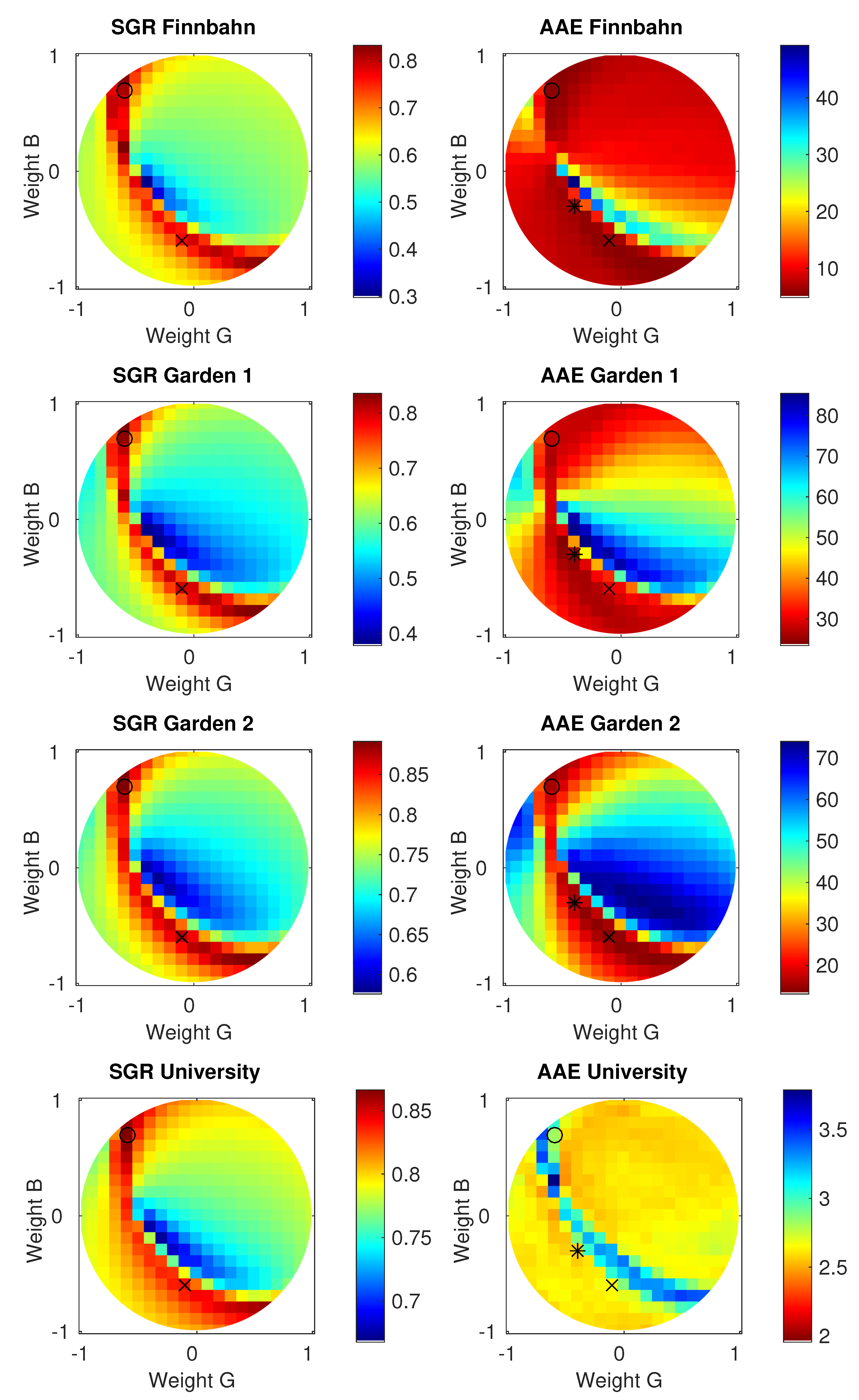
To further analyze the relationship between the SGR criterion and the MinWarping performance, we show results for the different databases separately. This enables deeper insights, as the databases differ significantly regarding the cloud cover. The database Finnbahn is characterized by a strong cloud cover, but changes in the cloud cover are almost unnoticeable throughout the database. The results for this database are shown in Figure 11 in the first row. The values for the SGR criterion show comparable properties to the values averaged over all databases. However, the average angular errors do not show the previously mentioned strong correlation with the SGR criterion. The region of linear combinations that reach a good homing performance is markedly larger compared to the results averaged over all databases. This can be explained by the characteristics of the database, which was captured under an overcast sky with barely visible changes in the cloud cover. Under these conditions, edges in the sky region do not disturb the image comparison, as they stay almost constant throughout the images. This effect is due to the limited duration of the image capturing process and the stable weather conditions. Nevertheless, the linear transformation with the best SGR value is a good choice as it results in low homing errors.
The databases Garden 1 and Garden 2 share similar characteristics: fast changing cloud cover throughout the image capturing processes. The results are shown in Figure 11 in the second and third row. Both databases show similar results to the effect that the best MinWarping performance coincides with the best SGR values. This reflects the assumption that variable cloud edges in the sky corrupt the homing performance. Both databases share a rapidly-changing, strong cloud cover, which results in high homing errors if the SGR criterion is low. In contrast, a high SGR value ensures a good homing performance.
The database university constitutes a special case, as the images captured are largely free of tilt and the sky is nearly cloudless. This leads to the results shown in Figure 11 in the last row. Here, the best values for SGR do not coincide with the best results of MinWarping. However, it has to be noticed that the differences in AAE values are comparably small (maximal 1.5°). Anyway, strong SGR values co-occur with moderately good home angle errors. The performance in the university database is similar to the Finnbahn database, but the conditions are different. In the university database, the sky was almost cloudless throughout the whole image capturing process. Thus, no misleading information in the sky is present, regardless of the factors of the linear transformation. Again, the choice of factors that result in a high SGR value still reaches a good homing performance. It is important to notice that the proposed linear transformation does not worsen the results if no misleading information in the sky is present.
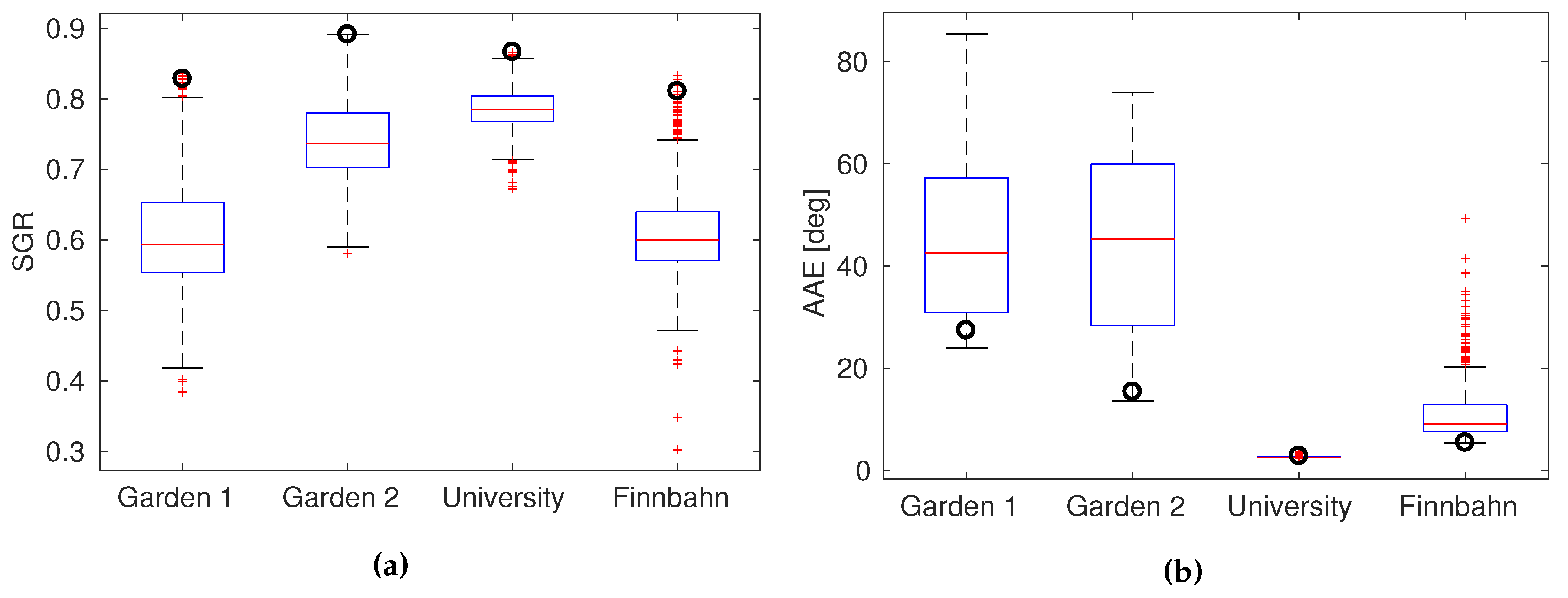
So far, all images were used as a basis for studying the relationship between the SGR criterion and the MinWarping performance. To show the generalization ability of the proposed method, we performed tests based on the principle of cross-validation. Our data are atypical for standard cross-validation, as they are organized in databases that each contain dependent images due to the spatial layout of the databases. We take this dependency of the data into account by performing a group-based cross-validation. This is separated into two experiments: (1) cross-validation of the SGR criterion; (2) cross-validation of the AAE based on the SGR criterion. The results for the SGR criterion are shown in Figure 12a. For this analysis, we split the data into a training and a test set in the following way: one database is retained as test set, and all other databases form the training set. This is repeated in such a way that each database is selected as the test set once. The label of each boxplot denotes the database used as the test set, and the data visualized as the boxplot is the set of SGR values reached by computing the SGR criterion for each parameter combination within this database (sampled as described in Section 3.2). For each test database, the circle marks the SGR value that is reached within this database by using the best parameter combination resulting from the training set. The graph shows that a high SGR criterion in the training set generalizes to a high SGR criterion in the test set. In other words, the selection of the best parameter combination based on the SGR criterion in a training set is an adequate choice for an unfamiliar environment.
In Figure 12b, the same cross-validation method is visualized with regard to homing results. Here, the parameter combination reaching the highest SGR value in the training set is used for computing the associated AAE in the test set (marked by a circle). The boxplot for each database visualizes the range of all possible AAE values throughout all parameter combinations. It is clearly visible that the selection based on the training set results in a nearly optimal performance regarding the homing performance in an unfamiliar environment.
These experiments support the proposed method in which the search for an optimal SGR value is used to find a linear color transformation that improves the homing performance. For all databases, the plot shows that a specific set of weights selected by optimizing the SGR criterion on a training set results in a nearly optimal AAE value in the test set. As the databases cover substantially different environments, the results demonstrate the generalization ability of the proposed method to unfamiliar environments.
6.3. Comparison with Alternative Methods
In this section, we describe visual homing experiments based on the proposed linear transformation (), which achieved the best sky-to-ground ratio in the experiments in Section 6.1 and compare it with three alternative approaches (described in Section 4.3).
To analyze the effect of misleading information in the sky region, we use manually-created mask images, which indicate the sky and ground region of the images. These mask images are used in additional experiments to remove the information in the sky region after the edge-filtering step. Applying MinWarping on these edge-filtered images allows us to investigate the effect of the information in the sky region.
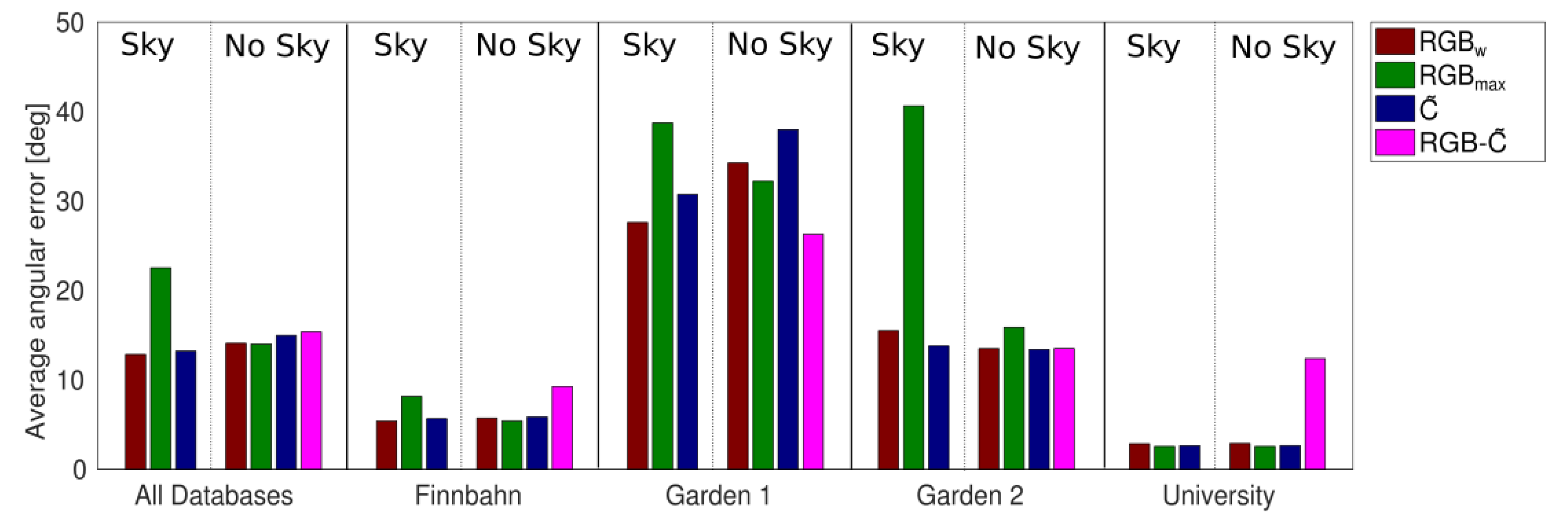
The results of MinWarping experiments on differently-filtered input are shown in more detail in Figure 13 averaged over all databases and additionally for each database separately in terms of AAE values in degrees. For these experiments, the value was set to 5.0 (see Section 6.4 for details). As a consequence, the left part of the figure (labeled “all databases”) illustrates the same results as Figure 14 for .
Averaged over all databases, the proposed transformation reaches the lowest errors, followed by the channel. The worst results are reached by using the method without taking into account the edges in the sky. Blackening of the sky in the method by using manually-created masks leads to a marked reduction of the errors. This sky blackening results in comparable results for all three methods, which supports the assumption that the specific kind of edge detection is not important for MinWarping; crucial is the elimination of misleading information in the sky. For the proposed method and the method, additional blackening of the sky region even worsens the results. This effect is probably caused by the design of the experiments, where changes in cloud cover are not present in all pairs of snapshots and current views. In some cases, the remaining information in the sky region using the and method could support the homing method. However, for the method, the misleading information obviously outweighs the supportive information. This effect should disappear in cross-database tests, where the sky never holds supportive information. Moreover, this effect is purely theoretical, because no manually-created masks for the sky blackening are available in real scenarios.
Instead of using manually-created masks, we additionally display the results obtained by using the contrast enhanced channel to compute a sky-ground mask and use this sky-ground mask to blacken the sky in the method (denoted as ). This approach is similar to the one used in [49,50], but differs to the extent that a different thresholding method is used. The results show that this approach improves the overall error compared to the method for the databases, but reaches worse results than the proposed method or . This effect occurs due to errors in the sky-ground separation, which could be identified in multiple images. We did not further investigate this effect, as the blackening of the sky with a correct mask (created manually) showed no improvement compared to the or methods. Therefore, it is not conducive to improve the thresholding, but preferable to use the proposed or channel without thresholding. In Figure 10 and Figure 11, the sampled linear factors closest to the -factors are marked by a cross. This explains the good homing performance of the -channel, as the -factors produce a high SGR value; however, other factors reach even higher values.
Differentiated consideration of the results in the individual databases allows for a deeper understanding of the analyzed methods. In particular, the results of the database university stand out as they differ from the other databases. In this database, the performance of all methods except the thresholded channel using Otsu’s thresholding show comparable results. Manual blackening of the sky does not show a noticeable effect on the homing performance, which can be explained by the characteristic of this database, which was collected under an almost cloudless sky. However, even under these conditions, the channel is a good choice. The large errors for the method are due to errors in the thresholding, which occurred when the white university building was visible against the bright sky. In this constellation, the university building was mistakenly classified as sky. This kind of error also occurred in the database Finnbahn when the Sun was shining through foliage. Overall, the applied Otsu’s thresholding tends to misclassify ground regions as sky, which is critical for the databases Finnbahn and university, but at the same time improves the homing performance in the databases Garden 1 and Garden 2, where overhanging bushes and trees complicate the homing process. In this context, misclassifying these overhanging ground regions as sky improves the homing performance compared to manual sky blackening. In contrast to Otsu’s thresholding, we decided to classify ambiguous regions in the manually-created masks as ground, e.g., canopy in front of bright sunshine. As a consequence, all regions containing ground elements are preserved when applying these masks, but also sky regions may still be present.
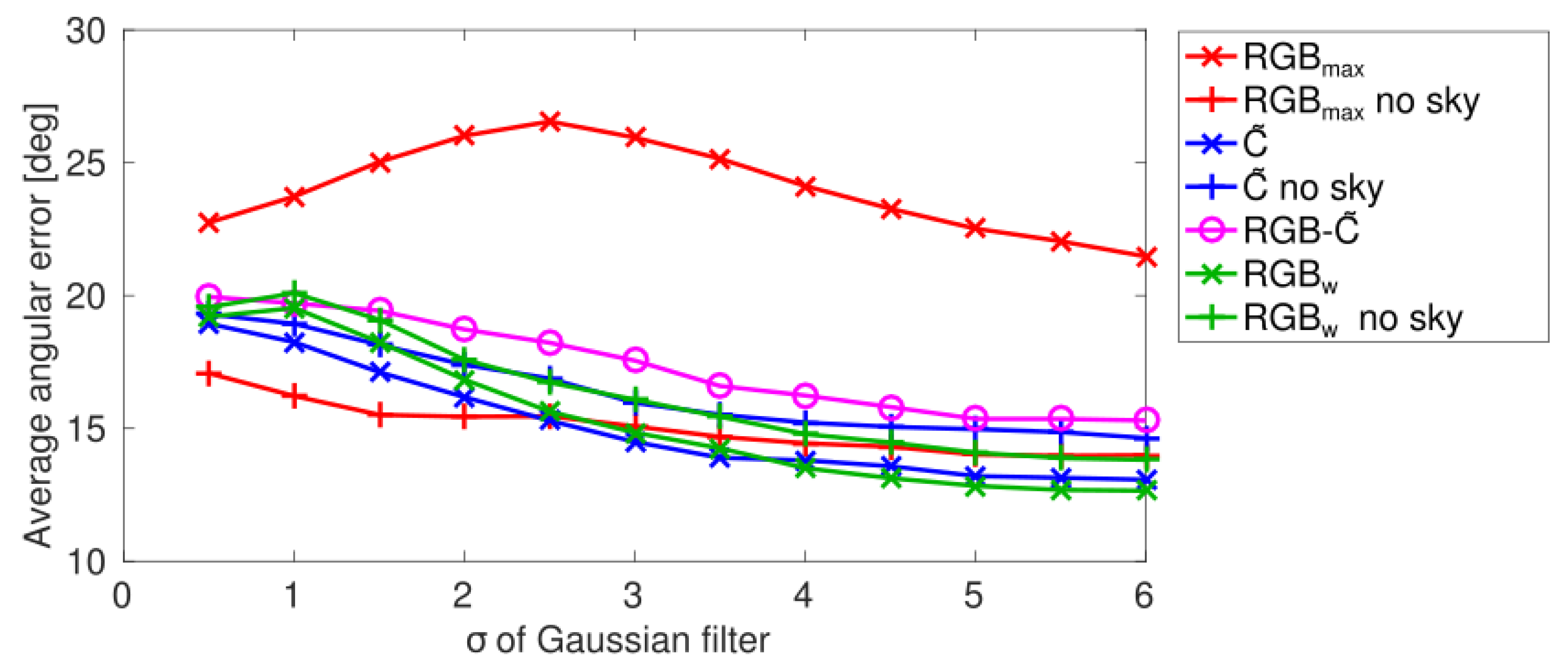
6.4. Influence of Low-Pass Parameter on Homing Performance
For the above comparison of the proposed method to alternative methods, the low-pass parameter was fixed to . This choice was made based on tests of the MinWarping performance on edge-filtered images using all above-mentioned alternative edge-filtering methods with different values for . The average angular errors (AAE) shown in Figure 14 are computed as averaged values over all grid databases. As can be seen, increasing of , which results in stronger low-pass filtered edge images, increases the MinWarping performance for all but one method. For the images filtered with the method, the homing performance gets worse up to and improves again for further increasing values. For , the MinWarping performance remains on approximately the same level for all methods, except . Based on these results, we choose as an appropriate value.
In Figure 14, the annotation “no sky” means that the sky region was removed from the edge-filtered images by using the manually-created masks.
7. Conclusions
That misleading information in the sky region deteriorating the performance of MinWarping is clearly visible in the results of the experiments using as the input. In a typical application of homing, no mask for deleting the sky region is available. Therefore, the proposed linear transformation shows promising properties for applications in outdoor environments. On the one hand, in the presence of changing cloud cover in the sky region, the homing procedure based on edge-filtered images performs significantly better than MinWarping on alternative input. On the other hand, when no misleading information in the sky is present, the homing procedure on edge-filtered images reaches comparable results to the homing procedure on alternative inputs. The method reaches comparable results to regarding the homing performance. This is in agreement with the assumption that high SGR values result in good homing performance and the fact that lies within the region of high SGR values (see Figure 10 where the region approximately corresponding to is marked by a cross).
Taken all together, we could show that a linear transformation of RGB input, which reaches a high SGR value used as input for MinWarping, significantly improves the homing performance. On the basis of the currently available databases, the highest SGR value does not result in the best homing performance, rather high SGR values form a region of potentially suitable parameter combinations. A broader data pool might possibly further restrict the suitable parameter combinations.
Based on the comparison of the results from with artificially-masked alternatives, we draw the conclusion that the suppression of edges within the sky region is a superior approach to thresholding using an optimized channel for thresholding (e.g., ). Even though we used nearly perfect masks (created manually), the masked alternatives reached worse performance than the suppression approach in the proposed method . Therefore, it is not conducive to improve the thresholding step within this context, but to use the proposed method directly and make the thresholding step redundant.
8. Future Work
As a part of future work, the factors of the linear transformation could be further optimized by including additional images in the SGR evaluation. Images captured with other cameras could stabilize the result and are planned in the future. Furthermore, the analysis of MinWarping performance in outdoor environments needs to be extended by cross-database tests, which we plan to collect in the short term. Therefore, databases will be acquired in the same places under different conditions, e.g., morning, noon and evening, or even on different days.
We analyzed the performance using MinWarping as the holistic homing method. The promising properties of the linearly-transformed channel might also improve other homing methods, for example feature-based approaches. In feature-based approaches, the proposed method might prevent the detection of features in the sky, which would otherwise result in outliers that have to be rejected in a subsequent outlier rejection step and thus increases the computation time.
To improve the overall performance of MinWarping in outdoor images, further research is in progress: problems occur when objects are located directly above the camera, which leads to strong distortions in the mapping to a rectangular view and additionally violates the assumptions of the MinWarping method. Furthermore, a deeper analysis of the effect of occlusions and change in altitude has to be performed. Additional research is needed to investigate the effect of the proposed linear transformation in the context of feature-based approaches.
Acknowledgments
The authors thank Dario Differt, Bielefeld University, for the implementation of the software to compute the ground truth data for the experiments. This work was supported by Deutsche Forschungsgemeinschaft (Grant No. MO 1037/10-1). Deutsche Forschungsgemeinschaft had no direct role in the creation of this work, nor the decision to submit it for publication.
Author Contributions
Annika Hoffmann developed the method. Annika Hoffmann and Ralf Möller conceived of and designed the experiments. Annika Hoffmann performed the experiments, analyzed the data and wrote the paper. Ralf Möller adapted the code of MinWarping, and Annika Hoffmann added extensions.
Conflicts of Interest
The authors declare no conflict of interest.
Appendix A. Customized Otsu’s Thresholding
We use the adaptive thresholding method from [61] to segment the sky from the ground region. Computing the histogram, which is the first step in this adaptive thresholding method, directly on the fisheye image would result in a distorted histogram due to distortions of the fisheye image. Starting from a panoramic image, mapped using the calibration in [58], we consider the area that one pixel in the mapped image represents in the fisheye image. Therefore, we modified the histogram computation by introducing weights depending on the elevation angle in the mapped image. The sine relationship of elevation angle to weights in fisheye images is a consequence of the coordinate transform from spherical to Cartesian coordinates. This weighting reduces the influence of the upper image rows, which are strongly distorted due to the mapping function.
Each pixel in the image is defined by an azimuth angle and an altitude angle . The weight w depends on the altitude angle and is computed by . In this way, pixels at the top of the image are weakly weighted, whereas pixels at the bottom are strongly weighted (as we use ). This modified histogram is then used as input for the thresholding described in [61].
References
- Yang, J.; Chung, S.J.; Hutchinson, S.; Johnson, D.; Kise, M. Omnidirectional-Vision-Based Estimation for Containment Detection of a Robotic Mower. In Proceedings of the International Conference on Robotics and Automation (ICRA), Seattle, WA, USA, 26–30 May 2015; IEEE: Piscataway, NJ, USA, 2015; pp. 6344–6351. [Google Scholar]
- Matthies, L.; Xiong, Y.; Hogg, R.; Zhu, D.; Rankin, A.; Kennedy, B.; Hebert, M.; Maclachlan, R.; Won, C.; Frost, T.; et al. A Portable, Autonomous, Urban Reconnaissance Robot. Robot. Auton. Syst. 2002, 40, 163–172. [Google Scholar] [CrossRef]
- Cui, Y.; Ge, S.S. Autonomous Vehicle Positioning with GPS in Urban Canyon Environments. IEEE Trans. Robot. Autom. 2003, 19, 15–25. [Google Scholar]
- Filitchkin, P.; Byl, K. Feature-based Terrain Classification for LittleDog. In Proceedings of the International Conference on Intelligent Robots and Systems (IROS), Vilamoura, Portugal, 7–12 October 2012; IEEE: Piscataway, NJ, USA, 2012; pp. 1387–1392. [Google Scholar]
- Khan, Y.N.; Komma, P.; Zell, A. High Resolution Visual Terrain Classification for Outdoor Robots. In Proceedings of the International Conference on Computer Vision Workshops (ICCV Workshops), Barcelona, Spain, 6–13 November 2011; IEEE: Piscataway, NJ, USA, 2011; pp. 1014–1021. [Google Scholar]
- Nelson, R.C.; Aloimonos, J. Finding Motion Parameters from Spherical Motion Fields (or the Advantages of Having Eyes in the Back of Your Head). Biol. Cybern. 1988, 58, 261–273. [Google Scholar] [CrossRef] [PubMed]
- Möller, R.; Krzykawski, M.; Gerstmayr, L. Three 2D–Warping Schemes for Visual Robot Navigation. Auton. Robot. 2010, 29, 253–291. [Google Scholar] [CrossRef]
- Churchill, D.; Vardy, A. An Orientation Invariant Visual Homing Algorithm. J. Intell. Robot. Syst. 2013, 71, 3–29. [Google Scholar] [CrossRef]
- Ramisa, A.; Goldhoorn, A.; Aldavert, D.; Toledo, R.; de Mantaras, R.L. Combining Invariant Features and the ALV Homing Method for Autonomous Robot Navigation Based on Panoramas. J. Intell. Robot. Syst. 2011, 64, 625–649. [Google Scholar] [CrossRef]
- Goedemé, T.; Tuytelaars, T.; Van Gool, L.; Vanacker, G.; Nuttin, M. Feature Based Omnidirectional Sparse Visual Path Following. In Proceedings of the 2005 IEEE/RSJ International Conference on Intelligent Robots and Systems, Edmonton, AB, Canada, 2–6 August 2005; IEEE: Piscataway, NJ, USA, 2005; pp. 1806–1811. [Google Scholar]
- Liu, M.; Pradalier, C.; Pomerleau, F.; Siegwart, R. Scale-only Visual Homing from an Omnidirectional Camera. In Proceedings of the IEEE International Conference on Robotics and Automation (ICRA), Saint Paul, MN, USA, 14–18 May 2012; IEEE: Piscataway, NJ, USA, 2012; pp. 3944–3949. [Google Scholar]
- Vardy, A.; Möller, R. Biologically Plausible Visual Homing Methods Based on Optical Flow Techniques. Connect. Sci. 2005, 17, 47–89. [Google Scholar] [CrossRef]
- Mochizuki, Y.; Imiya, A. Featureless Visual Navigation Using Optical Flow of Omnidirectional Image Sequence. In Proceedings of the International Conference on Simulation, Modeling, and Programming for Autonomous Robots (SIMPAR), Venice, Italy, 3–7 November 2008; Volume 8, pp. 307–318. [Google Scholar]
- Zhu, Q.; Liu, C.; Cai, C. A Novel Robot Visual Homing Method Based on SIFT Features. Sensors 2015, 15, 26063–26084. [Google Scholar] [CrossRef] [PubMed]
- Fleer, D.; Möller, R. Comparing Holistic and Feature-based Visual Methods for Estimating the Relative Pose of Mobile Robots. Robot. Auton. Syst. 2017, 89, 51–74. [Google Scholar] [CrossRef]
- Möller, R.; Horst, M.; Fleer, D. Illumination Tolerance for Visual Navigation with the Holistic Min-Warping Method. Robotics 2014, 3, 22–67. [Google Scholar] [CrossRef]
- Möller, R. Column Distance Measures and Their Effect on Illumination Tolerance in MinWarping; Technical Report; Faculty of Technology, Computer Engineering Group, Bielefeld University: Bielefeld, Germany, 2016. [Google Scholar]
- Raguram, R.; Frahm, J.M.; Pollefeys, M. A Comparative Analysis of RANSAC Techniques Leading to Adaptive Real-time Random Sample Consensus. In Proceedings of the European Conference on Computer Vision, Marseille, France, 12–18 October 2008; Springer: Berlin/Heidelberg, Germany, 2008; pp. 500–513. [Google Scholar]
- Möller, R.; Krzykawski, M.; Gerstmayr-Hillen, L.; Horst, M.; Fleer, D.; de Jong, J. Cleaning Robot Navigation Using Panoramic Views and Particle Clouds as Landmarks. Robot. Auton. Syst. 2013, 61, 1415–1439. [Google Scholar] [CrossRef]
- Gerstmayr-Hillen, L.; Röben, F.; Krzykawski, M.; Kreft, S.; Venjakob, D.; Möller, R. Dense Topological Maps and Partial Pose Estimation for Visual Control of an Autonomous Cleaning Robot. Robot. Auton. Syst. 2013, 61, 497–516. [Google Scholar] [CrossRef]
- Kamboj, A.; Grewal, K.; Mittal, R. Color Edge Detection in RGB Color Space Using Automatic Threshold Detection. Int. J. Innov. Technol. Explor. Eng. (IJITEE) 2012, 1, 41–45. [Google Scholar]
- Nevatia, R. Color Edge Detector and Its Use in Scene Segmentation. IEEE Trans. Syst. Man Cybern. 1977, 7, 820–826. [Google Scholar]
- Chapron, M. A Chromatic Contour Detector Based on Abrupt Change Techniques. In Proceedings of the International Conference on Image Processing, Santa Barbara, CA, USA, 26–29 October 1997; Volume 3, pp. 18–21. [Google Scholar]
- Di Zenzo, S. A Note on the Gradient of a Multi-image. Comput. Vis. Graph. Image Process. 1986, 33, 116–125. [Google Scholar] [CrossRef]
- Niu, L.; Li, W. Color Edge Detection Based on Direction Information Measure. In Proceedings of the 2006 6th World Congress on Intelligent Control and Automation, Dalian, China, 21–23 June 2006; IEEE: Piscataway, NJ, USA, 2006; Volume 2, pp. 9533–9536. [Google Scholar]
- Fan, J.; Aref, W.G.; Hacid, M.S.; Elmagarmid, A.K. An Improved Automatic Isotropic Color Edge Detection Technique. Pattern Recognit. Lett. 2001, 22, 1419–1429. [Google Scholar] [CrossRef]
- Carron, T.; Lambert, P. Color Edge Detector Using Jointly Hue, Saturation and Intensity. In Proceedings of the IEEE International Conference on Image Processing, Austin, TX, USA, 13–16 November 1994; IEEE: Piscataway, NJ, USA, 1994; Volume 3, pp. 977–981. [Google Scholar]
- Shiozaki, A. Edge Extraction Using Entropy Operator. Comput. Vis. Graph. Image Process. 1986, 36, 1–9. [Google Scholar] [CrossRef]
- Chen, X.; Chen, H. A Novel Color Edge Detection Algorithm in RGB Color Space. In Proceedings of the IEEE 10th International Conference on Signal Processing, Beijing, China, 24–28 October 2010; IEEE: Piscataway, NJ, USA, 2010; pp. 793–796. [Google Scholar]
- Zhao, J.; Xiang, Y.; Dawson, L.; Stewart, I. Color Image Edge Detection Based on Quantity of Color Information and its Implementation on the GPU. In Proceedings of the 23rd IASTED International Conference on Parallel and Distributed Computing and Systems (PDCS’11), Dallas, TX, USA, 14–16 December 2011; pp. 116–123. [Google Scholar]
- Wesolkowski, S.; Jernigan, E. Color Edge Detection in RGB Using Jointly Euclidean Distance and Vector Angle. In Proceedings of the IAPR Vision Interface Conference, Trois-Rivières, QC, Canada, 19–21 May 1999; pp. 9–16. [Google Scholar]
- Dutta, S.; Chaudhuri, B.B. A Color Edge Detection Algorithm in RGB Color Space. In Proceedings of the International Conference on Advances in Recent Technologies in Communication and Computing, ARTCom’09, Kottayam, Kerala, India, 27–28 October 2009; IEEE: Piscataway, NJ, USA, 2009; pp. 337–340. [Google Scholar]
- Cumani, A. Edge Detection in Multispectral Images. CVGIP: Graph. Models Image Process. 1991, 53, 40–51. [Google Scholar] [CrossRef]
- Garcia, P.; Pla, F.; Gracia, I. Detecting Edges in Colour Images Using Dichromatic Differences. In Proceedings of the Seventh International Conference on Image Processing and its Applications (Conf. Publ. No. 465), Manchester, UK, 13–15 July 1999; IET: Stevenage, UK, 1999; Volume 1, pp. 363–367. [Google Scholar]
- Scharcanski, J.; Venetsanopoulos, A.N. Edge Detection of Color Images Using Directional Operators. IEEE Trans. Circuits Syst. Video Technol. 1997, 7, 397–401. [Google Scholar] [CrossRef]
- Trahanias, P.E.; Venetsanopoulos, A.N. Vector Order Statistics Operators as Color Edge Detectors. IEEE Trans. Syst. Man Cybern. Part B (Cybernetics) 1996, 26, 135–143. [Google Scholar] [CrossRef] [PubMed]
- Yang, K.; Gao, S.; Li, C.; Li, Y. Efficient Color Boundary Detection with Color-opponent Mechanisms. In Proceedings of the IEEE Conference on Computer Vision and Pattern Recognition, Portland, OR, USA, 23–28 June 2013; pp. 2810–2817. [Google Scholar]
- Koschan, A.; Abidi, M. Detection and Classification of Edges in Color Images. IEEE Signal Process. Mag. 2005, 22, 64–73. [Google Scholar] [CrossRef]
- Mittal, A.; Sofat, S.; Hancock, E. Detection of Edges in Color Images: A Review and Evaluative Comparison of State-of-the-art Techniques. In Proceedings of the Autonomous and Intelligent Systems: Third International Conference, AIS 2012, Aveiro, Portugal, 25–27 June 2012; Springer: Berlin/Heidelberg, Germany, 2012; pp. 250–259. [Google Scholar]
- Zhu, S.Y.; Plataniotis, K.N.; Venetsanopoulos, A.N. Comprehensive Analysis of Edge Detection in Color Image Processing. Opt. Eng. 1999, 38, 612–625. [Google Scholar]
- Walia, S.S.; Singh, G. Color Based Edge Detection Techniques—A Review. Int. J. Eng. Innov. Technol. 2014, 3, 297–301. [Google Scholar]
- Differt, D.; Möller, R. Spectral Skyline Separation: Extended Landmark Databases and Panoramic Imaging. Sensors 2016, 16, 1614. [Google Scholar] [CrossRef] [PubMed]
- Differt, D.; Möller, R. Insect models of Illumination-invariant Skyline Extraction from UV and Green Channels. J. Theor. Biol. 2015, 380, 444–462. [Google Scholar] [CrossRef] [PubMed]
- Möller, R. Insects Could Exploit UV-green Contrast for Landmark Navigation. J. Theor. Biol. 2002, 214, 619–631. [Google Scholar] [CrossRef] [PubMed]
- Kollmeier, T.; Röben, F.; Schenck, W.; Möller, R. Spectral Contrasts for Landmark Navigation. J. Opt. Soc. Am. A 2007, 24, 1–10. [Google Scholar] [CrossRef]
- Bazin, J.C.; Kweon, I.; Demonceaux, C.; Vasseur, P. Dynamic Programming and Skyline Extraction in Catadioptric Infrared Images. In Proceedings of the IEEE International Conference on Robotics and Automation ICRA’09, Kobe, Japan, 12–17 May 2009; IEEE: Piscataway, NJ, USA, 2009; pp. 409–416. [Google Scholar]
- Shen, Y.; Wang, Q. Sky Region Detection in a Single Image for Autonomous Ground Robot Navigation. Int. J. Adv. Robot. Syst. 2013, 10. [Google Scholar] [CrossRef]
- Thurrowgood, S.; Soccol, D.; Moore, R.J.; Bland, D.; Srinivasan, M.V. A Vision Based System for Attitude Estimation of UAVs. In Proceedings of the International Conference on Intelligent Robots and Systems IROS, St. Louis, MO, USA, 10–15 October 2009; IEEE: Piscataway, NJ, USA, 2009; pp. 5725–5730. [Google Scholar]
- Pepperell, E.; Corke, P.; Milford, M. Towards Persistent Visual Navigation Using SMART. In Proceedings of the Australasian Conference on Robotics and Automation. ARAA, Sydney, Australia, 2–4 December 2013. [Google Scholar]
- Pepperell, E.; Corke, P.I.; Milford, M.J. All-environment Visual Place Recognition with SMART. In Proceedings of the IEEE International Conference on Robotics and Automation (ICRA), Hong Kong, China, 31 May–7 June 2014; IEEE: Piscataway, NJ, USA, 2014; pp. 1612–1618. [Google Scholar]
- Shafer, S.A. Using Color to Separate Reflection Components. Color Res. Appl. 1985, 10, 210–218. [Google Scholar] [CrossRef]
- Gevers, T.; Stokman, H. Classifying Color Edges in Video into Shadow-geometry, Highlight, or Material Transitions. IEEE Trans. Multimed. 2003, 5, 237–243. [Google Scholar] [CrossRef]
- Martin, D.R.; Fowlkes, C.C.; Malik, J. Learning to Detect Natural Image Boundaries Using Local Brightness, Color, and Texture Cues. IEEE Trans. Pattern Anal. Mach. Intell. 2004, 26, 530–549. [Google Scholar] [CrossRef] [PubMed]
- Papari, G.; Petkov, N. Edge and Line Oriented Contour Detection: State of the Art. Image Vis. Comput. 2011, 29, 79–103. [Google Scholar] [CrossRef]
- Arbelaez, P.; Maire, M.; Fowlkes, C.; Malik, J. Contour Detection and Hierarchical Image Segmentation. IEEE Trans. Pattern Anal. Mach. Intell. 2011, 33, 898–916. [Google Scholar] [CrossRef] [PubMed]
- Bista, S.; Varshney, A. Global Contours; Technical Report; Computer Science Department, University of Maryland: College Park, MD, USA, 2010. [Google Scholar]
- Debevec, P.E.; Malik, J. Recovering High Dynamic Range Radiance Maps from Photographs. In Proceedings of the 24th Annual Conference on Computer Graphics and Interactive Techniques, SIGGRAPH ’97, Los Angeles, CA, USA, 3–8 August 1997; ACM Press/Addison-Wesley Publishing Co.: New York, NY, USA, 1997; pp. 369–378. [Google Scholar]
- Scaramuzza, D.; Martinelli, A.; Siegwart, R. A Toolbox for Easily Calibrating Omnidirectional Cameras. In Proceedings of the 2006 IEEE/RSJ International Conference on Intelligent Robots and Systems, IROS, Beijing, China, 9–15 October 2006; pp. 5695–5701. [Google Scholar]
- Umbaugh, S.E. Computer Vision and Image Processing: A Practical Approach Using CVIPtools, 1st ed.; Prentice Hall PTR: Upper Saddle River, NJ, USA, 1997. [Google Scholar]
- Möller, R. A SIMD Implementation of the MinWarping Method for Local Visual Homing; Technical Report; Computer Engineering Group, Bielefeld University: Bielefeld, Germany, 2016. [Google Scholar]
- Otsu, N. A Threshold Selection Method from Gray-level Histograms. IEEE Trans. Syst. Man Cybern. 1979, 9, 62–66. [Google Scholar] [CrossRef]
Figure 1.
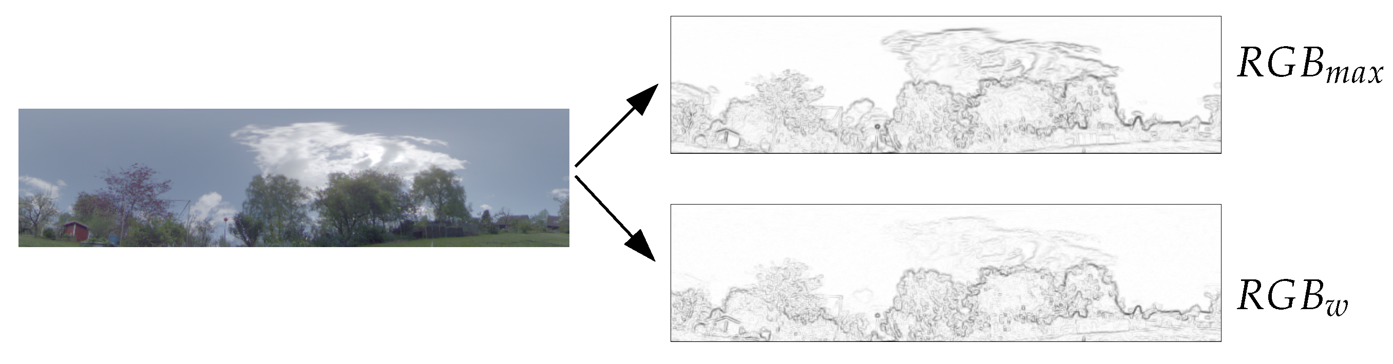
Example of the proposed edge-detection method. (Left) Input HDR color image from a panoramic camera mapped to a rectangular view (chosen from the database Garden 1). (Upper right) Prewitt-filtered image computed by applying the standard Prewitt filter on each RGB channel independently, followed by a maximum operation. (Lower right) Edge-filtered image using the proposed linear color transformation followed by a standard Prewitt filter on the transformed channel (RGB weighted). For better visualization, the edge-filtered images are shown with inverted colors. In the Prewitt-filtered image applied to the standard RGB channels, the clouds show distinct edge responses, whereas these edges are noticeably less prominent in the transformed image.
Figure 1.
Example of the proposed edge-detection method. (Left) Input HDR color image from a panoramic camera mapped to a rectangular view (chosen from the database Garden 1). (Upper right) Prewitt-filtered image computed by applying the standard Prewitt filter on each RGB channel independently, followed by a maximum operation. (Lower right) Edge-filtered image using the proposed linear color transformation followed by a standard Prewitt filter on the transformed channel (RGB weighted). For better visualization, the edge-filtered images are shown with inverted colors. In the Prewitt-filtered image applied to the standard RGB channels, the clouds show distinct edge responses, whereas these edges are noticeably less prominent in the transformed image.

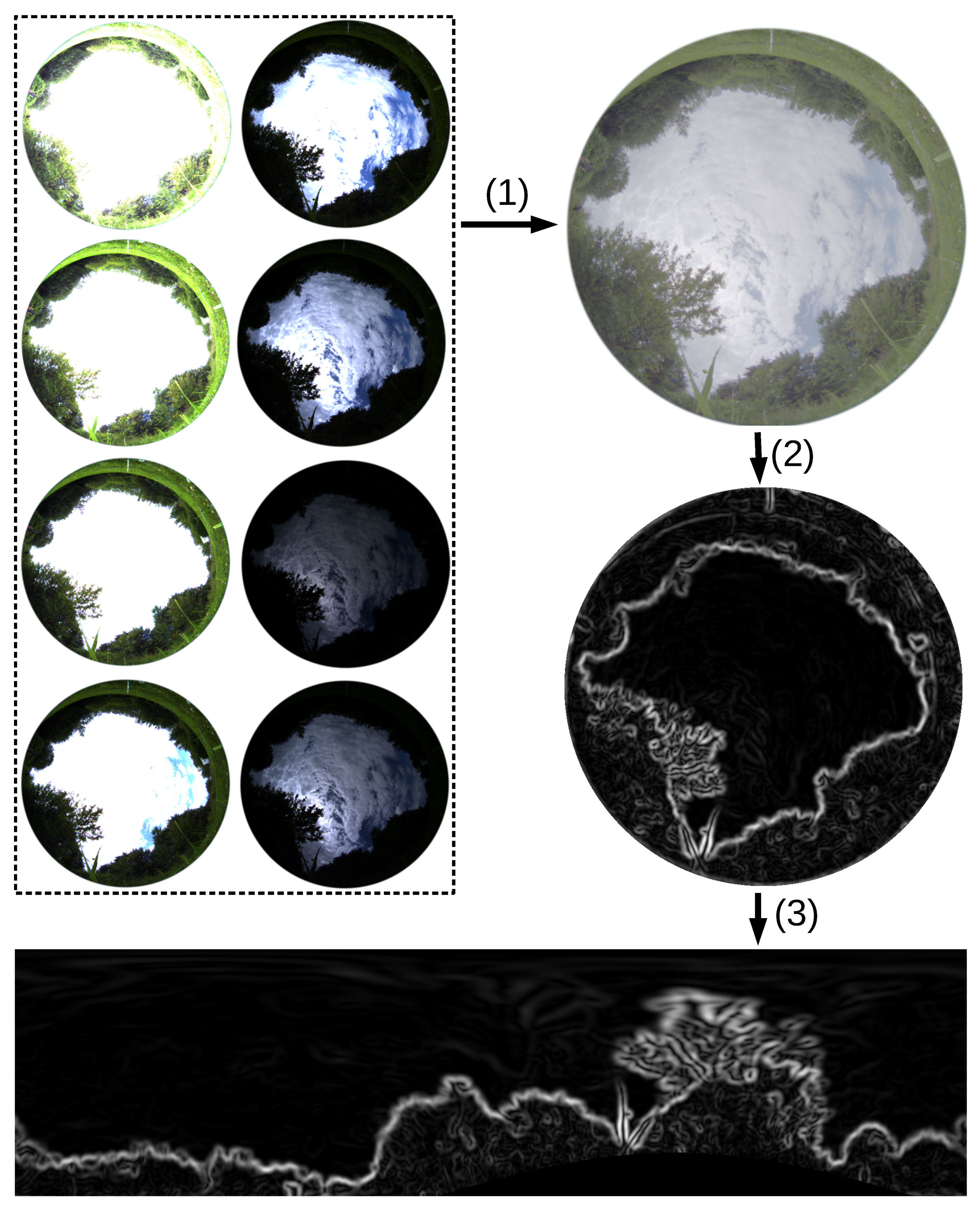
Figure 2.
Preprocessing pipeline: (1) An HDR image of size 1280 × 1024 is computed from a set of seven or eight low dynamic range images captured with different exposure times. (2) Gaussian filtering and edge detection are performed on the HDR image using a specific edge detection method. (3) The edge-filtered image is aligned to the gravity axis, mapped to a rectangular view and subsampled to a size of 288 × 72 pixels. The exemplary image is taken from the database Finnbahn, and as edge detection, the method is used.

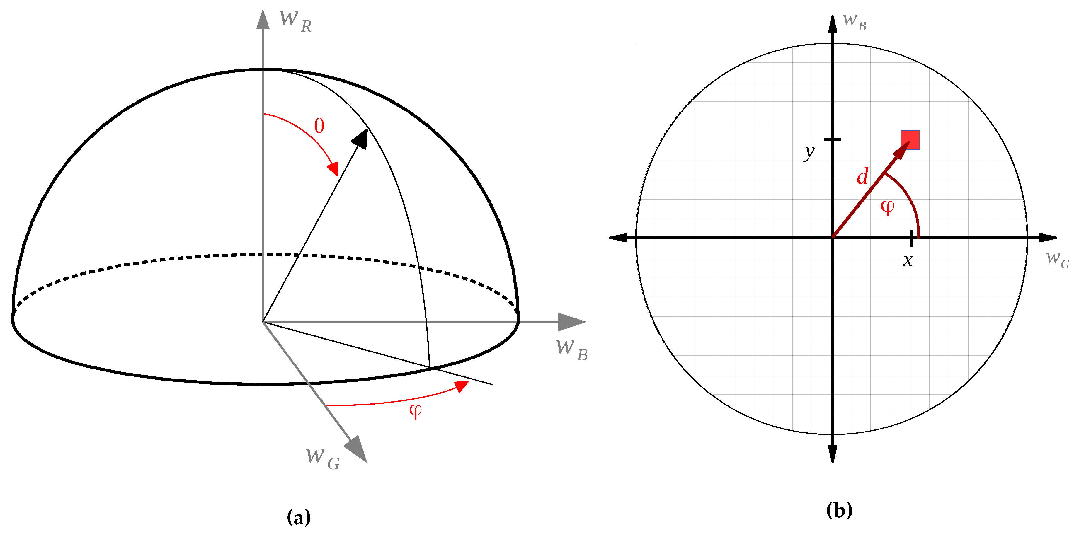
Figure 3.
(a) Parameter space for the linear combination of RGB channels. The factors , and of the linear combination define the axes of a spherical coordinate system. The relevant linear combinations lie on the surface of the upper hemisphere. The lower hemisphere is not relevant, because only absolute values of the edge detection are considered. (b) Visualization of the parameter space, which enables us to visualize the characteristic variables of the methods depending on the selected weight factors in a 2D plot.

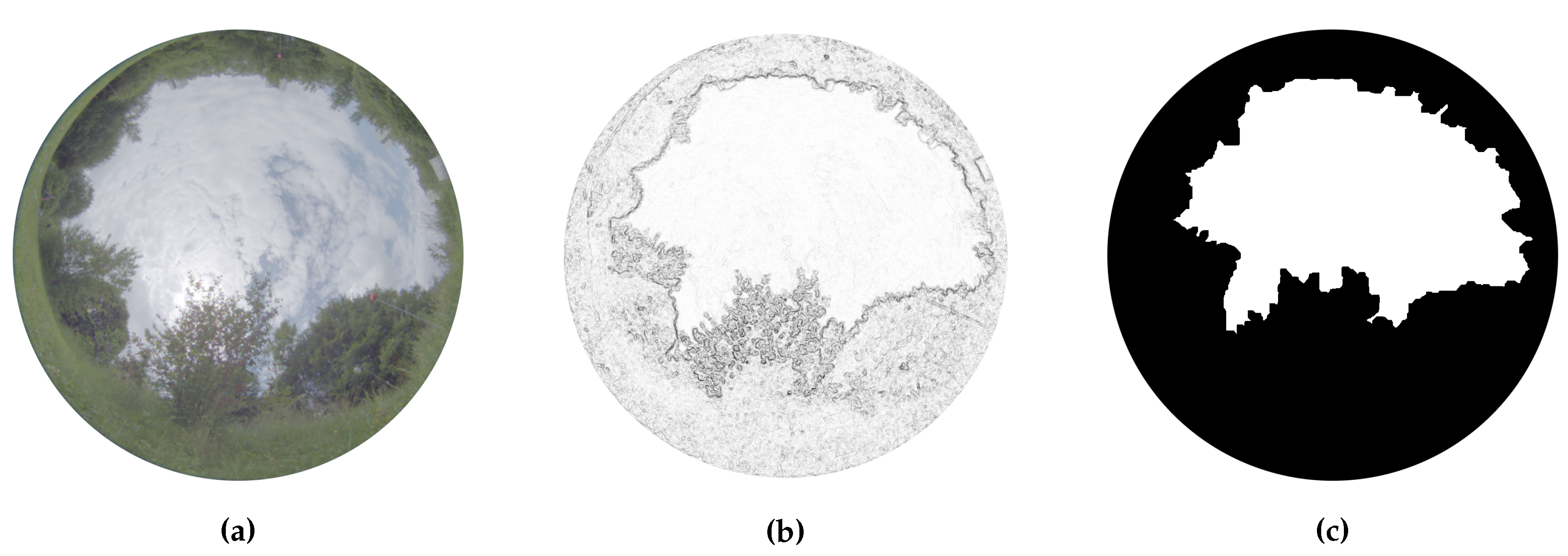
Figure 4.
Example image for analysis of the sky-to-ground ratio: (a) input color HDR image; (b) edge-filtered image; (c) mask image: the ground region is shown in black, and white represents the sky region. The image is taken from the database Finnbahn and edge-filtered using the method.
Figure 4.
Example image for analysis of the sky-to-ground ratio: (a) input color HDR image; (b) edge-filtered image; (c) mask image: the ground region is shown in black, and white represents the sky region. The image is taken from the database Finnbahn and edge-filtered using the method.

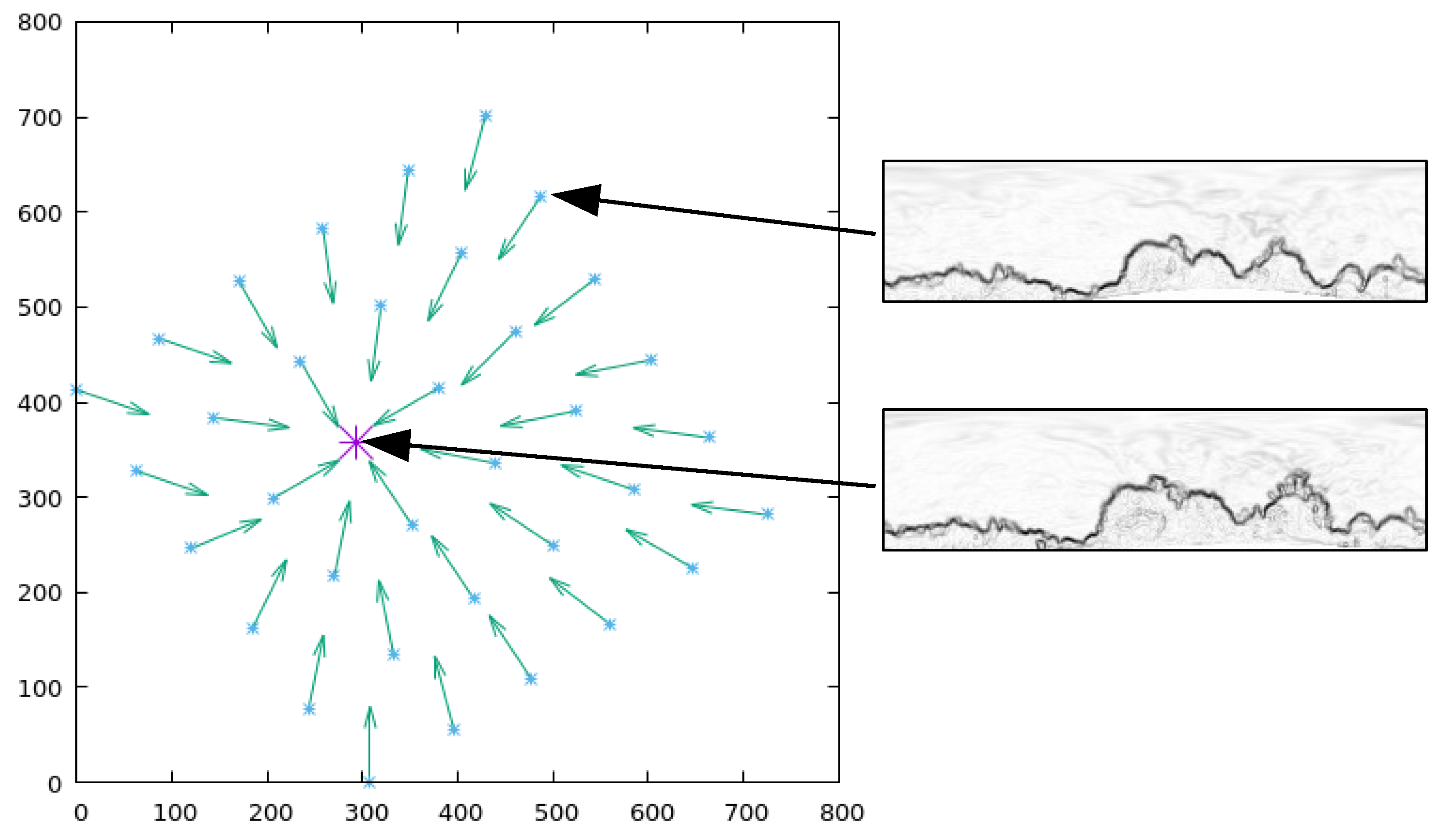
Figure 5.
Example of MinWarping experiments: One image (location marked in purple) is selected as the snapshot, and all other images are used as current views (blue). The computed home vectors are shown as green arrows. This example shows the setup of the Finnbahn database with images preprocessed using the method (). The edge-filtered images are shown with inverted colors for better visualization.

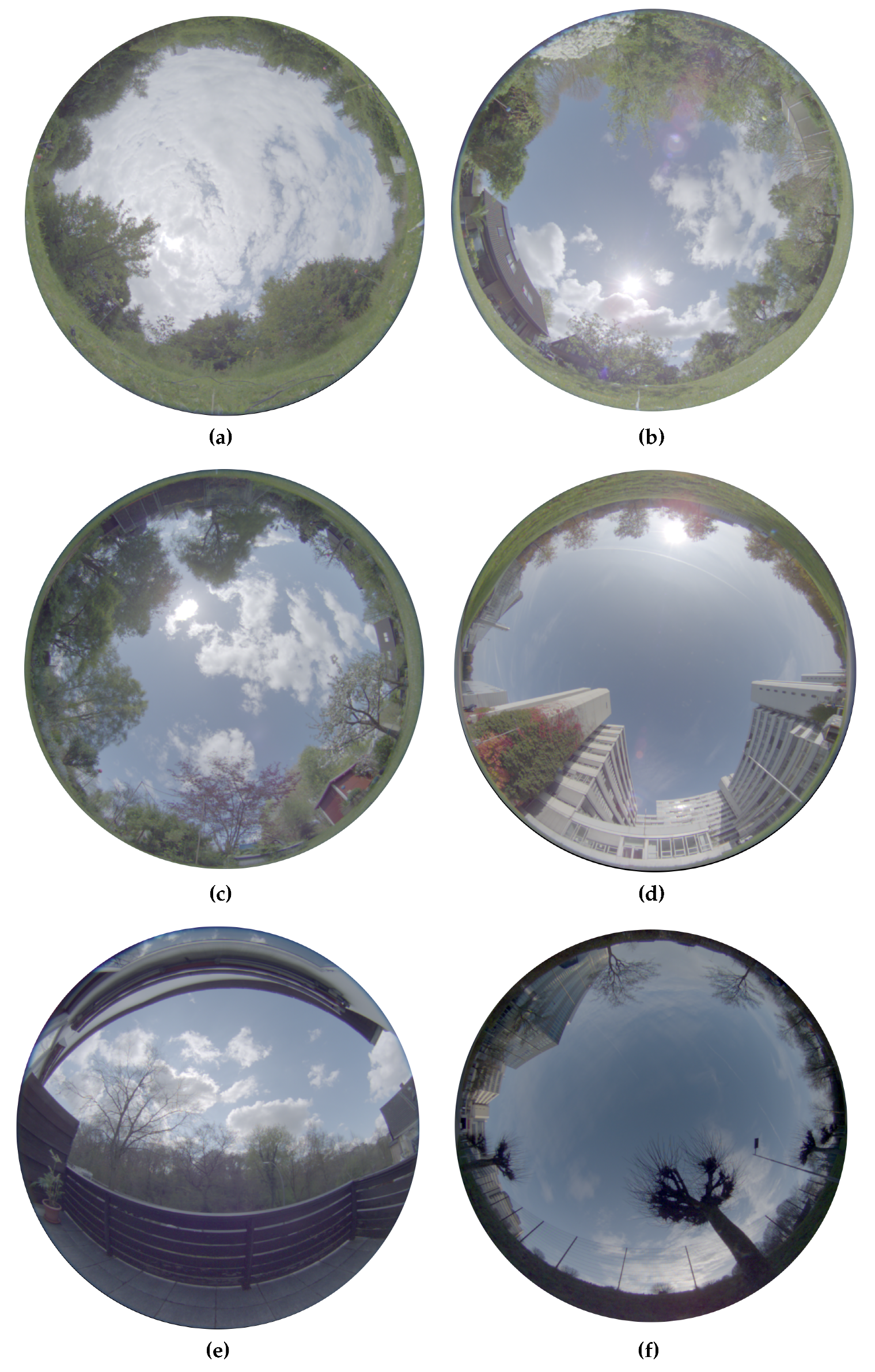
Figure 6.
Database environments: The images show the different environments in which the six databases were collected. The databases cover diverse environments under a wide range of dry weather conditions. (a) Finnbahn; (b) Garden 1; (c) Garden 2; (d) university; (e) balcony; (f) route.
Figure 6.
Database environments: The images show the different environments in which the six databases were collected. The databases cover diverse environments under a wide range of dry weather conditions. (a) Finnbahn; (b) Garden 1; (c) Garden 2; (d) university; (e) balcony; (f) route.

Figure 7.
Exemplary panoramic HDR images for each database. (a) Finnbahn; (b) Garden 1; (c) Garden 2; (d) university; (e) balcony; (f) route.
Figure 7.
Exemplary panoramic HDR images for each database. (a) Finnbahn; (b) Garden 1; (c) Garden 2; (d) university; (e) balcony; (f) route.

Figure 8.
Sky-to-ground ratio (SGR) and edge intensity (EI) of edge responses for different linear combinations of RGB channels. The color values show the SGR and EI criterion for a given linear combination. The surface of the hemisphere is projected onto a circle (see Figure 3b, and the description in Section 3.2). The selected parameter combination is marked by a circle, and the parameter combination closest to is marked by a cross.

Figure 9.
Bivariate histogram of SGR and EI values: high SGR values do coincide with the average or high EI values and are thus a reasonable choice.
Figure 9.
Bivariate histogram of SGR and EI values: high SGR values do coincide with the average or high EI values and are thus a reasonable choice.

Figure 10.
Relationship of sky-to-ground ratio and MinWarping performance averaged over all databases: (a) Sky-to-ground ratio for transformed RGB channels. (b) MinWarping performance in average angular errors (AAE) for transformed RGB channels. The color map for the AAE values is flipped to allow for a better comparison, since the goal is to reach low angular errors. The parameter combination with the highest SGR value is indicated by a circle, and the parameter combination closest to is marked by a cross. Additionally, the asterisk marks the parameter combination that reached the minimal AAE. (c) Scatter plot illustrating the strong, negative monotonic correlation between AAE and SGR values.

Figure 11.
Relationship of sky-to-ground ratio and MinWarping performance for different databases. (Left) sky-to-ground ratio for transformed RGB channels. (Right) MinWarping performance in average angular errors (AAE) for transformed RGB channels. The markers indicate the maximal SGR value (circle), the parameter combination closest to (cross) and the minimal AAE value (asterisk) averaged over all databases (see Figure 10).

Figure 12.
Group-based cross-validation: The data are divided into a test and a training set in such a way that the labeled database is selected as the test set and all other databases are used as the training set. (a) The boxplots show the range of the SGR criterion for each database as the test set with the edges of the box indicating the 25th () and 75th () percentiles, respectively. Values are defined as outliers if they fall below or above , where IQRdenotes the interquartile range, and the whiskers expand to the highest and lowest occurring values within these limits. The circle marks the SGR value in this database for the best parameter combination selected from the training set. (b) The boxplots show the range of the AAE-results for each database analogous to the boxplot parameters in (a). The circle indicates the AAE when the optimal parameter set from the training is used for the test database.

Figure 13.
Performance of MinWarping on differently-filtered input displayed averaged over all databases and for each database separately. The annotation “No Sky” means that the sky was blackened by using the manually-created masks for the methods , and , whereas the annotation “Sky” indicates that the images where used without further manipulation of the sky region. denotes the use of Otsu’s thresholding on the channel to blacken the sky in .

Figure 14.
Effect of the parameter used for Gaussian filtering on MinWarping performance. The results in average angular errors are averaged over all databases.
Figure 14.
Effect of the parameter used for Gaussian filtering on MinWarping performance. The results in average angular errors are averaged over all databases.


Table 1.
Parameters for MinWarping. NSAD, normalized sum of absolute differences.
| Image width | 288 |
| Image height | 72 |
| Vertical resolution of images | 0.022 (radians per pixel) |
| Number of scale planes | 9 |
| Number of search steps in direction | 96 |
| Number of search steps in direction | 96 |
| Maximal scale factor | 2.0 |
| Maximal threshold value | 2.5 |
| Distance measure | adapted NSAD |
| Elevation range | 0° to 70 ° |
© 2017 by the authors. Licensee MDPI, Basel, Switzerland. This article is an open access article distributed under the terms and conditions of the Creative Commons Attribution (CC BY) license (http://creativecommons.org/licenses/by/4.0/).
Share and Cite
MDPI and ACS Style
Hoffmann, A.; Möller, R. Cloud-Edge Suppression for Visual Outdoor Navigation. Robotics 2017, 6, 38. https://doi.org/10.3390/robotics6040038
AMA Style
Hoffmann A, Möller R. Cloud-Edge Suppression for Visual Outdoor Navigation. Robotics. 2017; 6(4):38. https://doi.org/10.3390/robotics6040038
Chicago/Turabian StyleHoffmann, Annika, and Ralf Möller. 2017. "Cloud-Edge Suppression for Visual Outdoor Navigation" Robotics 6, no. 4: 38. https://doi.org/10.3390/robotics6040038
Note that from the first issue of 2016, this journal uses article numbers instead of page numbers. See further details here.