Improving Sports Outcome Prediction Process Using Integrating Adaptive Weighted Features and Machine Learning Techniques

Abstract

Developing an effective sports performance analysis process is an attractive issue in sports team management. This study proposed an improved sports outcome prediction process by integrating adaptive weighted features and machine learning algorithms for basketball game score prediction. The feature engineering method is used to construct designed features based on game-lag information and adaptive weighting of variables in the proposed prediction process. These designed features are then applied to the five machine learning methods, including classification and regression trees (CART), random forest (RF), stochastic gradient boosting (SGB), eXtreme gradient boosting (XGBoost), and extreme learning machine (ELM) for constructing effective prediction models. The empirical results from National Basketball Association (NBA) data revealed that the proposed sports outcome prediction process could generate a promising prediction result compared to the competing models without adaptive weighting features. Our results also showed that the machine learning models with four game-lags information and adaptive weighting of power could generate better prediction performance.

1. Introduction

The sports market has proliferated at the beginning of the 21st century with new approaches and techniques such as streaming broadcasting, social media, and the global supply chain. With the growth of sports market value, sports team management attracted considerable attention and became a popular topic from researchers. For example, some studies established decision support methods to assist the teams’ decision of rookie draft [1,2]. Some research aimed to analyze the teams’ player selection and scouting policy [3,4]. Moreover, developing an effective sports performance analysis process such as determining the factors that affect the results of sports games [2,5] and predicting games or players’ performance [6,7] is one of the most attractive issues in sports teams’ management.

Sports outcome prediction is a significant part of the sports performance analysis process. It influences many sports markets, such as sports team management, betting, and customer service, since the accurate prediction of sports game outcome provides detailed information for managing strategy reference, bookmakers, and attraction for viewers. For example, a team supervisor, such as a general manager (GM), is facing numerous vital decisions on the daily management of the team. The accurate prediction of future games provides the reference of marketing strategy to design specific fans’ service activities. Moreover, detail and accurate prediction provide GM and head coach vital information to decide the team’s starting lineup. The authors of [8] reviewed scientific papers using date mining techniques to predict the sport outcomes. They showed that the prediction performance of existing research is potentially improved by more future research. In [9], the authors review over 100 scientific papers related to using machine learning in sports outcome prediction. They pointed out that sport outcome predictions were most commonly using supervised machine learning techniques. The regression methods usually utilized to solve the score prediction object. They also suggested that using multiple machine learning algorithms in finding the optimal algorithms and finding patterns among data are two of the most important tasks to improve the prediction performance in the future research.

Therefore, sports outcome prediction became an attractive topic for researchers in different sports domains [10,11,12]. Among different sports, basketball games outcome prediction or forecasting is the most popular topic for researchers [8,9] since National Basketball Association (NBA) is the most welcoming sports league worldwide [13,14,15,16,17,18,19,20,21,22,23,24]. The existing basketball game outcome prediction can be classified in two primary directions: win/lose (W/L) prediction and game score prediction. Predicting the future game’s W/L is an essential issue for team staff, participants, and fans since W/L is the simplest way to determine the result of a team’s performance [13,14,15,16,17,18,19]. However, for technical analyst, betting bookers, and commentators, game score prediction provide more detailed information for stakeholders aforementioned [20,21,22,23,24]. This study proposed an improved sports outcome prediction process by integrating machine learning algorithms for NBA game score prediction.

Feature engineering is the process of domain experts that use data to create features that enhance the effectiveness of machine learning algorithms [25]. It is mainly computing the features which have the most significant effect on the effectiveness and accuracy of the proposed model [26]. Commonly used feature engineering methodologies contain technical analysis and statistical methodologies. Statistical methodologies aim at compression and dimension reduction. Technical analysis assumes that future incidents are correlated to some historical patterns. Moving average (MA) is the mathematical expression of historical data sets defined to describe specific characteristics of presumed hidden rules and is a valuable technical indicator for feature engineering [24,27]. Adaptive weighting (AW) is a promising method to improve the prediction model’s performance and applied in various areas [28,29,30]. To apply AW in the design of features, variables are given with different weightings to describe the effect of each variable on the designed features. In order to consider the different weightings of each feature, the inverse distance weighting (IDW) method is used in the outcome of the proposed sports prediction process.

IDW method is a deterministic spatial interpolation method. It presumes that any specific pair of data points’ attribute values are associated with each other, but their association is inversely related to the range between the two data points. A practical methodology to model the spatial interaction between two data points is to modify the distance weight by a power of exponential function. The exponential function is widely used when predicting the unknown attribute values at specific data points in applying the IDW method [31,32,33,34].

Machine learning algorithms have been successfully used to build effective prediction models for different applications in the various area [35,36,37,38,39,40,41]. There is relatively fewer research applying machine learning methods for NBA game outcomes prediction and NBA game final score prediction [16,17,18,19,20,21,22,23,24]. Therefore, five machine learning methods, including classification and regression trees (CART) [42,43,44,45,46,47,48,49], random forest (RF) [50,51,52,53,54,55,56,57,58,59,60], stochastic gradient boosting (SGB) [24,45,52,61,62,63,64,65,66,67], eXtreme gradient boosting (XGBoost) [24,68,69,70,71,72,73], and extreme learning machine (ELM) [24,73,74,75,76,77], are used in this study for constructing an improved NBA game score prediction process, as they have been successfully used in various applications such as public security [36], manufacturing [37,38,39], and resource management [40,41].

CART is a statistical procedure often used as a regression tool to analyze continuous data [42,43,44,45,46,47,48,49]. The approach of RF has shown excellent performance in the dataset with large amount of variables and observations by combining several randomized decision tress and aggregates their predictions by averaging [50,51,52,53,54,55,56,57,58,59,60]. SGB is a hybrid method that merging boosting and bagging techniques, and the input data are selected by random sampling at each stage of the steepest gradient algorithm-based boosting procedure [24,45,52,61,62,63,64,65,66,67]. XGBoost is a supervised machine learning algorithm developed from a scalable end-to-end gradient tree boosting principle [24,68,69,70,71,72,73]. ELM is a single-hidden-layer feedforward neural network that randomly selects the input weights and systematically calculates the output weights of the network [24,73,74,75,76,77].

In the proposed NBA game score prediction process, the most acceptable and accessible statistics of an NBA game are collected and used as initial variables. Then, using these variables as input, the feature engineering method is used to construct the designed feature based on the interaction of game-lag information and adaptive weighting of variables. These designed features are then applied to the five machine learning methods, i.e., CART, RF, SGB, XGBoost, and ELM, to build prediction models. Finally, by evaluating the performance of prediction models, the sufficient selection of game-lag information, and proper adaptive weighting of variables combination on features were identified.

This research is organized as follows: Section 1 presents the background and the concept of this study. Section 2 shows the brief introduction of machine learning techniques that were used in this research. Section 3 demonstrates the details of the outcome of the proposed sports prediction process. Section 4 gives the proposed sports outcome prediction process’s empirical results, followed by the Conclusions section.

2. Methodology

Five machine learning techniques involving CART, RF, SGB, XGBoost, and ELM are utilized in this study.

CART is a statistical procedure often used as a regression tool to analyze continuous data. CART can be concluded into three stages. The first stage involves developing the tree using a recursive partitioning technique to filter variables and split data points using a splitting criterion. After a large tree is produced, the second stage uses a pruning procedure that coordinates with a minimal cost complexity measure. The methodology’s last stage is identifying the optimal tree by corresponding with a tree yielding the lowest cross-validated or testing set error rate [42,43,44,45,46,47,48,49]. For modeling the CART model, the “rpart” R package of version 4.1-15 [78] with pruning strategy was used.

RF has provided promising performance as a general-purpose regression method. By combining several randomized decision trees and aggregates their predictions by averaging, the approach of RF has shown excellent performance in the dataset with large amount of variables and observations. It is also flexible enough to be implemented to large-scale task, is conveniently adapted to various ad hoc learning problems, and returns measures of variable importance [50,51,52,53,54,55,56,57,58,59,60]. The “randomForest” R package of version 4.6-14 [79] was used to construct the RF model.

SGB is a hybrid algorithm that merging boosting and bagging techniques. Data are filtered by random sampling at each phase of the steepest gradient method-based boosting process. SGB develops smaller trees at each stage of the boosting procedure instead of developing a full regression tree. Optimal data fractionation is computed by coordinate with a consequential process, and the residual of every fraction is obtained. The results are comprised to lower the sensitivity of these methods for target data [24,45,52,61,62,63,64,65,66,67]. The SGB model was constructed by the “gbm” R package of version 2.1.8 [80].

XGBoost commonly uses a tree-based supervised machine learning technique developed from a scalable end-to-end gradient tree boosting principle. A weak learner is developed to be optimistically correlated with the negative gradient of the loss function and refers to the entire model. XGBoost is a generalized gradient boosting decision tree applied by a new tree scanning method that reduces tree building time. XGBoost moderated overfitting to support arbitrary adaptable loss functions by regularization term [24,68,69,70,71,72,73]. The “xgboost” R package of version 1.3.2.1 [81] is used to construct the XGBoost model.

ELM is a single-hidden-layer feedforward neural network that randomly indicates the weighting of input and systematically calculates that weighting of the network’s output. ELM has a quicker model building time compared to the traditional feedforward network machine learning methods. ELM reduces common disadvantages found in gradient-based techniques [24,73,74,75,76,77]. The ELM model was constructed by the “elmNN” package version 1.0 [82]. The default used activation function in this package is radial basis.

All R packages were implemented in R software of version 3.6.2 [83]. The default setting of modeling strategy of each package is used. To find the best hyper-parameter set for building an effective prediction model, “caret” R package of version 6.0.84 [84] was implemented for tuning the important hyper-parameters of each machine learning algorithm.

3. Proposed Sports Outcome Prediction Process

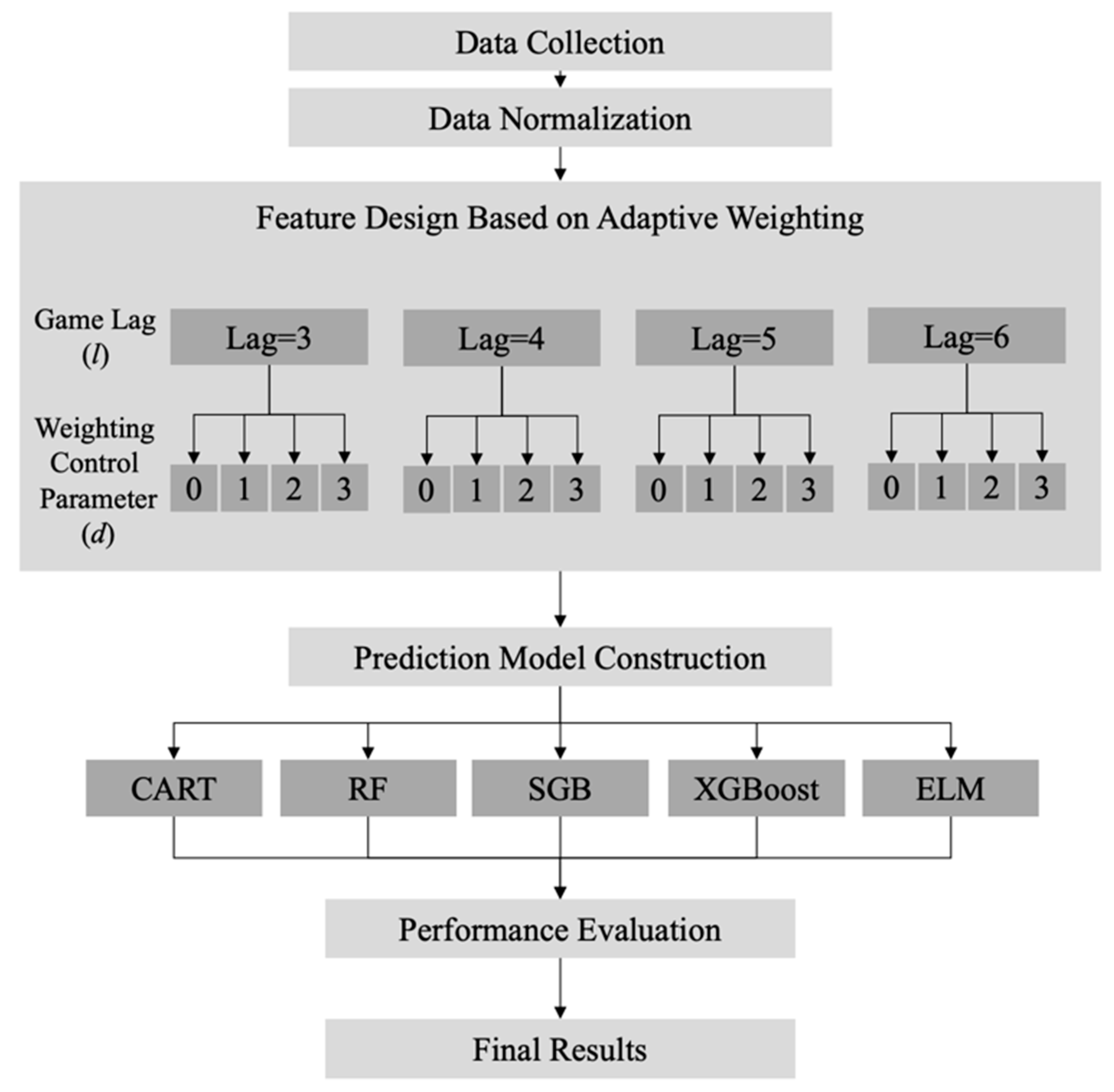
The adaptive weighting information was integrated into the feature design process in the proposed sports prediction process outcome. Then, the five machine learning algorithms are implemented to predict the final score of the NBA game using the designed features. The flowchart of the proposed process is shown in Figure 1.

Step 1: Data Collection

The first step is data collection. We acquired data from the basketball-reference website (https://www.basketball-reference.com, accessed on 15 March 2021) for every NBA 2018–2019 regular-season games. This NBA season consists of 1230 regular-season games, and each game has two teams (home team and away team) on the court. Each game presents two data points, one from home and another from the away team. Therefore, 2460 data points were collected and used in this study.

A total of 15 variables are collected and utilized in this research. One is the team’s final game score, and the remaining 14 are the most widely used statistics of the basketball game, including the team’s defensive and offensive performance.

Table 1. Variable Description.

Variables	Abbreviation	Description
$X_{1,t}$	2PA	2-Point Field Goal Attempts of a team in $t_{th }$ game
$X_{2,t}$	2P%	2-Point Field Goal Percentage of a team in $t_{th }$ game
$X_{3,t}$	3PA	3-Point Field Goal Attempts of a team in $t_{th }$ game
$X_{4,t}$	3P%	3-Point Field Goal Percentage of a team in $t_{th}$ game
$X_{5,t}$	FTA	Free Throw Attempts of a team in $t_{th}$ game
$X_{6,t}$	FT%	Free Throw Percentage of a team in $t_{th}$ game
$X_{7,t}$	ORB	Offensive Rebounds of a team in $t_{th }$ game
$X_{8,t}$	DRB	Defensive Rebounds of a team in $t_{th }$ game
$X_{9,t}$	AST	Assists of a team in $t_{th}$ game
$X_{10,t}$	STL	Steals of a team in $t_{th}$ game
$X_{11,t}$	BLK	Blocks of a team in $t_{th}$ game
$X_{12,t}$	TOV	Turnovers of a team in $t_{th }$ game
$X_{13,t}$	PF	Personal Fouls of a team in $t_{th}$ game
$X_{14,t}$	H/A	Home or Away game of a team in $t_{th}$ game
$Y_t$	Score	Team Score of a team in $t_{th }$ game

presents variable definitions. Variable $X_{i,t}$ is the i_th variable at the t_th game. Y_t is the team’s final score at the t_th game, which this research uses as the target variable. Since each team plays 82 games in the 2018–2019 NBA regular season and 14 variables were used in this study, variable $X_{i,t}$ can be defined as $1\le i\le 14, 1\le t\le 82$.

Step 2: Data Normalization

Data normalization is implemented before feature construction since each variable has different scales. The min-max normalization technique is used to transform a value $v$ of variable V to $v\prime$ in the range [0, 1] by using the following equation as a calculation:

$$X_{i,t}^{\prime }=\frac{X_{i,t}-min{X}_i}{max{X}_i-min{X}_i}$$

(1)

where $max{X}_i$ and $min{X}_i$ are the maximum and minimum values for the attribute $X_i$. Data normalization is implemented to ensure that larger input variable values will not influence smaller input variables values to reduce prediction errors.

Step 3: Feature Design based on Adaptive Weighting

This step aims to integrate adaptive weighting techniques into feature construction. We design our features for the prediction models based on the normalized variables shown in Table 1. This feature construction proceeds based on the interaction of two dimensions: game-lag information and the exponential power of adaptive weighting.

First, we define the game-lag information as “the n_th game before game t”. Researchers utilized the single game-lag information of up to six games for model construction in recent related research [14,15,16,17,18,19,20,21]. This research considers three to six game-lag information instead of considering only single game-lag information. Moreover, this research considers the moving average of the past statistic of a basketball game in order to be sufficient for evaluating a team’s performance. We calculate the mean value of a normalized variable within l game-lags to evaluate a team’s performance during a specific duration.

Second, it is crucial to understand that the nearest data point theoretically has more influence on the prediction unknown target. Therefore, this research designed the adaptive weighting method based on inverse-distance weighting (IDW) by integrating exponential power d as a weighting control parameter. The designed feature ${\overline{X}}_{i,t}^{l,d}$ can be described as follow:

$${\overline{X}}_{i,t}^{l,d}={\displaystyle \sum }_{n=1}^{l}A{W}_{n,d}^l\times X^{\prime }{}_{i,t-n}$$

(2)

and the adaptive weighting, $A{W}_{n,d}^l$, is calculated as follow:

$$A{W}_{n,d}^l=\frac{{\left(l-n+1\right)}^d}{{{\displaystyle \sum }}_1^l{n}^d}$$

(3)

where i = variables sequence (1 ≤ I ≤ 14), t = target game (1 ≤ t ≤ 82), l = game-lag information (3 ≤ l ≤ 6), d = weighting control parameter (0 ≤ d ≤ 3). Feature ${\overline{X}}_{i,t}^{l,d}$ is the designed i_th predictor variable at the t_th game with l game-lags based on d exponential power of adaptive weighting.

For instance, for the first normalized variable (i = 1), if we wish to design a feature considering four game-lag’s information (l = 3) with weighting control parameter d = 1 for the game No. 25 (or 25th game, t = 25) of a team, the values of the first variable in the previous three games are calculated as the designed feature. That is

$${\overline{X}}_{1,25}^{3,1}={\displaystyle \sum }_{n=1}^{3}A{W}_{n,1}^3\times X^{\prime }{}_{1,25-n}=A{W}_{1,1}^3\times X^{\prime }{}_{1,24}+A{W}_{2,1}^3\times X^{\prime }{}_{1,23}+A{W}_{3,1}^3\times X^{\prime }{}_{1,22}$$

(4)

where $A{W}_{1,1}^3=\frac{{\left(3-1+1\right)}^1}{1^1+2^1+3^1}=0.5$, $A{W}_{2,1}^3=\frac{{\left(3-2+1\right)}^1}{1^1+2^1+3^1}\approx 0.34$, and $A{W}_{3,1}^3=\frac{{\left(3-3+1\right)}^1}{1^1+2^1+3^1}\approx 0.16$. This instance can be found in Figure 2 as the line of d = 1. It can be observed in Figure 2 that the weighting distribution on the line of d = 0 will be equal with all the variables, which represents the simple average method. The weighting distribution of d = 0 is demonstrated as $A{W}_{1,0}^3=\frac{{\left(3-1+1\right)}^0}{1^0+2^0+3^0}\approx 0.33$, $A{W}_{2,0}^3=\frac{{\left(3-2+1\right)}^0}{1^0+2^0+3^0}\approx 0.33$, and $A{W}_{3,0}^3=\frac{{\left(3-3+1\right)}^0}{1^0+2^0+3^0}\approx 0.33$.

Figure 3 demonstrated the weighting distribution of four feature set under l = 4, Figure 4 illustrates the weighting distribution of four feature set under l = 5. Figure 5 shows the weighting distribution of four feature set under l = 6. Note that with the higher value of selected game-lag information, the nearest data point (t-1) weighting is not necessarily growing with it.

Most recent research using previous basketball game’s statistics to predict the outcome of basketball games construct the feature by using the simple average method [14,15,16,17,18,19,20,21] which is equal to setting weighting control parameter (d) = 0 in Equations (2) and (3). The weighting distribution of adaptive weighting method (d = 1, d = 2, and d = 3) allocates the most weighting on the nearest data point, i.e., the data point on t-1. The weighting of t-1 is growing with the higher of a weighting control parameter. On the other hand, the weighting of the farthest data point is allocated with the lowest weighting. The margin between the highest weighting and lowest weighting is increased with the higher weighting control parameter.

Step 4: Prediction Model Construction

In this phase, we construct a prediction model for predicting the final scores of the NBA games by using 14 designed features with five machine learning methods, namely CART, RF, SGB, XGBoost, and ELM. According to step3, each variable can be extended to 16 features which is the combination of four game-lags and four weighting control parameters. For modeling a machine learning prediction model, the 14 designed variables with a specific game-lag and weighting control parameter are used as predictor variables. That is, for a machine learning method, 16 prediction models will be can be generated for evaluating the effects of different game-lags and different weighting control parameters based on prediction performance.

That is, using the designed features with a specific game-lag and weighting control parameter (${\overline{X}}_{i,t}^{l,d}$) to predict the final score of a game ($Y_t^{}$) can be expressed as the following equation:

$$Y_t^{}=f\left({\overline{X}}_{i,t}^{l,d}\right)$$

(5)

where $1\le i \le 14,3\le l \le 6,7\le t \le 82,0\le d\le 3,\forall i,t,l,d\in \mathbb{N}.$

Note that all 14 designed features (1 ≤ i ≤ 14) were used with three to six game-lags’ information (3 ≤ l ≤ 6) and with zero to three of the weighting control parameters (0 ≤ d ≤ 3) for each $Y_t^{}$. As aforementioned, this research compares the prediction performance with different weighting control parameters under a different selection of game-lag information. Since we use up to six games’ information as our game-lag information, the season’s first six games are skipped (7 ≤ t ≤ 82).

Step 5: Performance Evaluation

This research aims to discover the influence of patterns from previous games to the target game and is a cross-sectional analysis. Therefore, this study utilized the cross-validation method which is commonly used in sports outcome prediction [85,86,87] to estimate the performance of the proposed prediction process. Moreover, according to [13], cross-validation method can be a better validation method in sports outcome prediction. We replicate 10-fold cross-validation 100 times. This study used the root mean square error (RMSE) as the indicator to evaluate the prediction performance of each method as it is one of the most commonly used prediction performance indicators [88,89] and has been used as a standard statistical metric to measure model performance in meteorology, air quality, and climate researches [90,91,92]. Many sports outcome-prediction research used only RMSE as the prediction performance indicator [93,94,95]. Therefore, this research use RMSE as prediction performance indicator. It is calculated as Equation (6):

$$\mathrm{RMSE}=\sqrt[]{\frac{1}{n}{\displaystyle \sum }_{i=1}^n{e}_i^2}$$

(6)

where n is the sample size, and $e_i$ represents the error of predictions.

Step 6: Final Results

In the final phase, after the performance evaluation of the prediction models, the best production process can be obtained. Based on the best prediction process, we shall determine the sufficient selection of game-lag information and practical preference of exponential power on adaptive weighting.

4. Empirical Results

In this research, each NBA game’s statistics of both competing teams in the 2018–2019 regular season were collected to evaluate the performance of the proposed basketball game score prediction process.

Figure 6 shows the prediction performance of each prediction model with different weighting control parameters (d) under game-lag (l) = 3. It can be observed that prediction performance varies from different weighting control parameters. Each prediction model reach its best prediction performance with weighting control parameter(d) = 1, CART (RMSE = 12.2611), RF (RMSE = 12.2159), SGB (RMSE = 12.1671), XGBoost (RMSE = 12.2736), and ELM (RMSE = 12.4846). Moreover, with the higher weighting control parameter (d = 2 and d = 3), the prediction performance is not necessarily better with all the prediction models.

Figure 7 demonstrates the performance metrics of prediction models with different weighting control parameter (d) under game-lag (l) = 4. It is clear that every prediction model reaches its best prediction performance with weighting control parameter (d) = 1, such as CART (RMSE = 11.7564), RF (RMSE = 11.6303), SGB (RMSE = 11.5586), XGBoost (RMSE = 11.6941), and ELM (RMSE = 11.8020).

Figure 8 presents the prediction performance of prediction models with different weighting control parameters (d) under game-lag (l) = 5. Every prediction model reaches its best prediction performance with weighting control parameter (d) = 1, such as CART (RMSE = 12.4316), RF (RMSE = 12.1525), SGB (RMSE = 12.2448), XGBoost (RMSE = 12.3145), and ELM (RMSE = 12.6748). Note that the prediction performance became worse with the increase of weighting control parameters from 1 to 3.

Figure 9 shows the prediction performance of prediction models with different weighting control parameter (d) under game-lag (l) = 6. Every prediction model reaches its best prediction performance with weighting control parameter (d) = 1, such asCART (RMSE = 12.0896), RF (RMSE = 12.0245), SGB (RMSE = 12.0293), XGBoost (RMSE = 11.9898), and ELM (RMSE = 12.2520).

Table 2. Performance metrics of the proposed prediction scheme.

Game-Lag Selection	Methods, Mean (SD)	Weighting Control Parameter
		d = 0	d = 1	d = 2	d = 3
Lag = 3	CART	12.5396(0.3290)	12.2611(0.3306)	13.0188(0.4692)	12.8924(0.2148)
	RF	12.4307(0.2905)	12.2159(0.3745)	12.6226(0.4834)	12.5646(0.2224)
	SGB	12.4195(0.2497)	12.1671(0.3266)	12.4670(0.4863)	12.5261(0.2312)
	XGBoost	12.3062(0.2659)	12.2736(0.3173)	12.6042(0.4987)	12.6124(0.2152)
	ELM	12.5172(0.3316)	12.4846(0.3203)	13.0403(0.4648)	12.9261(0.1883)
Lag = 4	CART	12.3434(0.4804)	11.7564(0.2878)	12.9753(0.4243)	12.4579(0.3524)
	RF	11.9571(0.3822)	11.6303(0.2608)	12.6935(0.4393)	12.2696(0.3283)
	SGB	12.0481(0.4366)	11.5586(0.2914)	12.6784(0.3873)	12.1120(0.3628)
	XGBoost	12.0491(0.4159)	11.6941(0.2787)	12.6785(0.4090)	12.0791(0.3280)
	ELM	12.2817(0.3972)	11.8020(0.2599)	12.9334(0.3991)	12.4511(0.3401)
Lag = 5	CART	13.1326(0.2213)	12.4316(0.2403)	12.8013(0.2307)	13.0725(0.4351)
	RF	12.6148(0.2084)	12.1525(0.2545)	12.5351(0.3057)	12.8432(0.4818)
	SGB	12.6969(0.2198)	12.2448(0.2307)	12.6745(0.1237)	12.9750(0.3807)
	XGBoost	12.7785(0.1925)	12.3145(0.2506)	12.6760(0.1069)	12.8648(0.3881)
	ELM	13.0344(0.1970)	12.6748(0.2529)	13.0100(0.1896)	13.0235(0.4071)
Lag = 6	CART	12.3738(0.2968)	12.0896(0.3365)	12.9175(0.3717)	12.4925(0.3025)
	RF	12.3614(0.2805)	12.0245(0.4672)	12.9398(0.3260)	12.3072(0.3375)
	SGB	12.1067(0.3232)	12.0293(0.3484)	12.9223(0.2830)	12.0876(0.2995)
	XGBoost	12.1655(0.3143)	11.9898(0.3171)	12.8547(0.3208)	12.2934(0.3074)
	ELM	12.3923(0.2942)	12.2520(0.3485)	13.0727(0.2992)	12.3416(0.3309)

summarizes the mean and standard deviation (SD) of RMSE of each machine learning method with different weighting control parameters (d) under a different scenario of game-lag information (l). It can be observed that every model reaches their best prediction performance with weighting control parameter value of level one (d = 1) under the scenario of selecting four as game-lag information (l = 4), such as CART (RMSE = 11.7564), RF (RMSE = 11.6303), SGB (RMSE = 11.5586), XGBoost (RMSE = 11.6941), and ELM (RMSE = 11.8020). Compared to the methods with a simple average weighting feature (d = 0), the models with a weighting control parameter value of level one (d = 1) provide promising effects on the improvement of prediction performance. Note that with the higher value of the weighting control parameter, the prediction performance is not necessarily encouraged.

However, it also can be observed in Table 2 that the difference between models’ results is relatively small. The confident interval (CI) is calculated in order to determine whether the difference between models and feature combinations is significant.

Table 3. Confident intervals of performance metrics of the proposed prediction scheme.

Game-Lag Selection	Methods, CI	Weighting Control Parameter
		d = 0	d = 1	d = 2	d = 3
Lag = 3	CART	(12.6041, 12.4751)	(12.3259, 12.1963)	(13.1107, 12.9268)	(12.9345, 12.8503)
	RF	(12.4876, 12.3737)	(12.2893, 12.1425)	(12.7173, 12.5279)	(12.6081, 12.5210)
	SGB	(12.4684, 12.3705)	(12.2311, 12.1030)	(12.5623, 12.3717)	(12.5715, 12.4808)
	XGBoost	(12.3583, 12.2541)	(12.3357, 12.2114)	(12.7020, 12.5065)	(12.6545, 12.5702)
	ELM	(12.5822, 12.4522)	(12.5473, 12.4218)	(13.1314, 12.9492)	(12.9630, 12.8892)
Lag = 4	CART	(12.4376, 12.2493)	(11.8128, 11.7000)	(13.0584, 12.8921)	(12.5269, 12.3888)
	RF	(12.0320, 11.8822)	(11.6814, 11.5791)	(12.7796, 12.6074)	(12.3612, 12.2325)
	SGB	(12.1337, 11.9625)	(11.6157, 11.5015)	(12.7543, 12.6025)	(12.1832, 12.0409)
	XGBoost	(12.1306, 11.9675)	(11.7487, 11.6395)	(12.7586, 12.5983)	(12.1434, 12.0148)
	ELM	(12.3595, 12.2038)	(11.8529, 11.7511)	(13.0116, 12.8552)	(12.5187, 12.3845)
Lag = 5	CART	(13.1759, 13.0892)	(12.4787, 12.3845)	(12.8465, 12.7561)	(13.1578, 12.9872)
	RF	(12.6557, 12.5740)	(12.2024, 12.1026)	(12.5951, 12.4752)	(12.9377, 12.7488)
	SGB	(12.7400, 12.6538)	(12.2901, 12.1996)	(12.6987, 12.6502)	(13.0496, 12.9003)
	XGBoost	(12.8162, 12.7408)	(12.3636, 12.2654)	(12.6970, 12.6551)	(12.9409, 12.7888)
	ELM	(13.0730, 12.9958)	(12.7244, 12.6253)	(13.0471, 12.9728)	(13.1033, 12.9437)
Lag = 6	CART	(112.4319, 12.3156)	(12.1555, 12.0236)	(12.9903, 12.8446)	(12.5518, 12.4332)
	RF	(12.4163, 12.3064)	(12.1161, 11.9329)	(13.0037, 12.8759)	(12.3734, 12.2411)
	SGB	(12.1700, 12.0433)	(12.0975, 11.9610)	(12.9778, 12.8668)	(12.1463, 12.0289)
	XGBoost	(12.2271, 12.1039)	(12.0520, 11.9276)	(12.9175, 12.7918)	(12.3537, 12.2332)
	ELM	(12.4499, 12.3346)	(12.3203, 12.1837)	(13.1314, 13.0141)	(12.4064, 12.2767)

shows the confident intervals of each machine learning method with different weighting control parameters and different game-lag information. It reveals that the prediction performance of weighting control parameter of one and a game-lag of four significantly outperformed other feature combinations used as an input predictor for the five machine learning algorithms. It also can be observed from Table 2 and Table 3 that although the SGB with d = 1 and l = 4 slightly outperforms the competing methods in this feature combination, the difference is not statistically significant. Therefore, these five machine learning algorithms provide a promising prediction performance by using designed features with a weighting control parameter of one and game-lag of four as predictor variables.

Moreover, from Table 2 and Table 3, it can be seen that the models’ prediction performance with weighting control parameter of two and three are not as good as a model with a weighting control parameter of one. The potential cause of this circumstance can be explained as, by observing Figure 2, Figure 3, Figure 4 and Figure 5, the weighting of each data point is linearly declining with a weighting control parameter of one while the weighting of each data point is non-linearly declining with a weighting control parameter of two and three. The weighting distribution curve with a linear decline represents a team’s performance over the last few games are linearly and stable, referable to the target game t. Contrarily, for the weighting distribution curve with a non-linear decline, a team’s performance over the last few games is unstable and is relatively not referable. That is, the influence of the performance in nearer games are enhanced and subsequently too high, while the performance in farther games are declining too fast. However, since NBA is a professional team sport, coach and players are well-trained to adapt themselves by substitute the cooling players with hot-hand players, using time-outs to adjust their condition, or provide and receive assistance with teammates to cover the unstable performance. Therefore, the weighting distribution with a linear decline with a farther data point which represents the stable team performance is a more appropriate distribution for the prediction on outcome of team sports.

5. Conclusions

This research integrated the designed features using the adaptive weighted method and CART, RF, SGB, XGBoost, and ELM machine learning methods for constructing an effective sports outcome prediction process. The designed features were based on the interaction of three to six pieces of game-lags information, and four different levels of the adaptive weighting of variables were generated. This study collected data from all the regular-season games of the NBA 2018–2019 seasons as illustrative examples. Empirical results showed that the proposed sports outcome prediction could generate a promising prediction result compared to the competing models without adaptive weighting features. All the five machine learning methods reach their best prediction performance with the weighting control parameter value of level one and four pieces of game-lags information. Although SGB in this feature combination slightly outperforms the competing methods, the difference is not statistically significant. Therefore, these five machine learning algorithms provide promising prediction performance by using feature combination with weighting control parameter of one and game-lag of four to generate the input features.

Integrating the machine learning methods with adaptive weighting based on feature selection and combination strategies to generate an improved version of the proposed scheme is worthy further investigated since the exploration of feature selection results is an important task in the implementation of machine learning algorithms in sports outcome prediction [9]. Thus, modifying the proposed scheme to adapt to feature selection techniques could be one of the future research directions. Moreover, exploring the performance of the proposed scheme with more NBA seasons’ data could be also a future research direction.

References

- Arel, B.; Tomas, M.J., III. The NBA Draft: A Put Option Analogy. J. Sports Econ. 2012, 13, 223–249. [Google Scholar] [CrossRef]
- Pollard, R. Evidence of a Reduced Home Advantage When a Team Moves to a New Stadium. J. Sports Sci. 2002, 20, 969–973. [Google Scholar] [CrossRef]
- Yang, C.H.; Lin, H.Y. Is There Salary Discrimination by Nationality in the NBA?: Foreign Talent or Foreign Market. J. Sports Econ. 2012, 13, 53–75. [Google Scholar] [CrossRef]
- Kopkin, N. Tax Avoidance: How Income Tax Rates Affect the Labor Migration Decisions of NBA Free Agents. J. Sports Econ. 2012, 13, 571–602. [Google Scholar] [CrossRef]
- Pollard, R.; Pollard, G. Long-Term Trends in Home Advantage in Professional Team Sports in North America and England (1876–2003). J. Sport Sci. 2005, 23, 337–350. [Google Scholar] [CrossRef] [PubMed]
- Zhang, S.; Lorenzo, A.; Gómez, M.Á.; Mateus, N.; Gonçalves, B.S.V.; Sampaio, J. Clustering Performances in the NBA According to Players’ Anthropometric Attributes and Playing Experience. J. Sports Sci. 2018, 36, 2511–2520. [Google Scholar] [CrossRef]
- Morgulev, E.; Azar, O.H.; Bar-Eli, M. Searching for Momentum in NBA Triplets of Free Throws. J. Sports Sci. 2020, 38, 390–398. [Google Scholar] [CrossRef] [PubMed]
- Haghighat, M.; Rastegari, H.; Nourafza, N.; Branch, N.; Esfahan, I. A review of data mining techniques for result prediction in sports. Adv. Comput. Sci. Int. J. 2013, 2, 7–12. [Google Scholar]
- Horvat, T.; Job, J. The use of machine learning in sport outcome prediction: A review. Wiley Interdiscip. Rev. Data Min. Knowl. Discov. 2020, 10, e1380. [Google Scholar] [CrossRef]
- Morgulev, E.; Azar, O.H.; Lidor, R. Sports Analytics and the Big-Data Era. Int. J. Data Sci. Anal. 2018, 5, 213–222. [Google Scholar] [CrossRef]
- Musa, R.M.; Majeed, A.P.A.; Taha, Z.; Chang, S.W.; Nasir, A.F.A.; Abdullah, M.R. A Machine Learning Approach of Predicting High Potential Archers by Means of Physical Fitness Indicators. PLoS ONE 2019, 14, e0209638. [Google Scholar] [CrossRef]
- Baboota, R.; Kaur, H. Predictive Analysis and Modelling Football Results using Machine Learning Approach for English Premier League. Int. J. Forecast. 2019, 35, 741–755. [Google Scholar] [CrossRef]
- Zuccolotto, P.; Manisera, M.; Sandri, M. Big Data Analytics for Modeling Scoring Probability in Basketball: The Effect of Shooting under High-Pressure Conditions. Int. J. Sports Sci. Coach. 2018, 13, 569–589. [Google Scholar] [CrossRef]
- Lam, M.W. One-Match-Ahead Forecasting in Two-Team Sports with Stacked Bayesian Regressions. J. Artif. Intell. Soft Comput. Res. 2018, 8, 159–171. [Google Scholar] [CrossRef] [Green Version]
- Horvat, T.; Havaš, L.; Srpak, D. The Impact of Selecting a Validation Method in Machine Learning on Predicting Basketball Game Outcomes. Symmetry 2020, 12, 431. [Google Scholar] [CrossRef] [Green Version]
- Loeffelholz, B.; Bednar, E.; Bauer, K.W. Predicting NBA Games using Neural Networks. J. Quant. Anal. Sports 2009, 5, 7. [Google Scholar] [CrossRef]
- Cheng, G.; Zhang, Z.; Kyebambe, M.N.; Kimbugwe, N. Predicting the Outcome of NBA Playoffs Based on the Maximum Entropy Principle. Entropy 2016, 18, 450. [Google Scholar] [CrossRef]
- Pai, P.F.; Chang-Liao, L.H.; Lin, K.P. Analyzing Basketball Games by a Support Vector Machines With Decision Tree Model. Neural Comput. Appl. 2017, 28, 4159–4167. [Google Scholar] [CrossRef]
- Li, Y.; Wang, L.; Li, F. A Data-Driven Prediction Approach for Sports Team Performance and Its Application to National Basketball Association. Omega 2021, 98, 102123. [Google Scholar] [CrossRef]
- Song, K.; Zou, Q.; Shi, J. Modelling the Scores and Performance Statistics of NBA Basketball Games. Commun. Stat.-Simul. Comput. 2018, 49, 2604–2616. [Google Scholar] [CrossRef]
- Thabtah, F.; Zhang, L.; Abdelhamid, N. NBA Game Result Prediction Using Feature Analysis and Machine Learning. Ann. Data Sci. 2019, 6, 103–116. [Google Scholar] [CrossRef]
- Huang, M.L.; Lin, Y.J. Regression Tree Model for Predicting Game Scores for the Golden State Warriors in the National Basketball Association. Symmetry 2020, 12, 835. [Google Scholar] [CrossRef]
- Song, K.; Gao, Y.; Shi, J. Making Real-Time Predictions for NBA Basketball Games by Combining the Historical Data and Bookmaker’s Betting Line. Phys. A Stat. Mech. Appl. 2020, 547, 124411. [Google Scholar] [CrossRef]
- Chen, W.-J.; Jhou, M.-J.; Lee, T.-S.; Lu, C.-J. Hybrid Basketball Game Outcome Prediction Model by Integrating Data Mining Methods for the National Basketball Association. Entropy 2021, 23, 477. [Google Scholar] [CrossRef]
- Domingos, P. A few useful things to know about machine learning. Commun. ACM 2012, 55, 78–87. [Google Scholar] [CrossRef] [Green Version]
- Zhang, C.; Cao, L.; Romagnoli, A. On the feature engineering of building energy data mining. Sustain. Cities Soc. 2018, 39, 508–518. [Google Scholar] [CrossRef]
- Long, W.; Lu, Z.; Cui, L. Deep learning-based feature engineering for stock price movement prediction. Knowl.-Based Syst. 2019, 164, 163–173. [Google Scholar] [CrossRef]
- Chen, Y.; Gao, D.; Nie, C.; Luo, L.; Chen, W.; Yin, X.; Lin, Y. Bayesian statistical reconstruction for low-dose X-ray computed tomography using an adaptive-weighting nonlocal prior. Comput. Med. Imaging Graph. 2009, 33, 495–500. [Google Scholar] [CrossRef]
- Pang, Y.; Peng, L.; Chen, Z.; Yang, B.; Zhang, H. Imbalanced learning based on adaptive weighting and Gaussian function synthesizing with an application on Android malware detection. Inf. Sci. 2019, 484, 95–112. [Google Scholar] [CrossRef]
- Yang, M.; Deng, C.; Nie, F. Adaptive-weighting discriminative regression for multi-view classification. Pattern Recognit. 2019, 88, 236–245. [Google Scholar] [CrossRef]
- Bartier, P.M.; Keller, C.P. Multivariate interpolation to incorporate thematic surface data using inverse distance weighting (IDW). Comput. Geosci. 1996, 22, 795–799. [Google Scholar] [CrossRef]
- Bekele, A.; Downer, R.G.; Wolcott, M.C.; Hudnall, W.H.; Moore, S.H. Comparative evaluation of spatial prediction methods in a field experiment for mapping soil potassium. Soil Sci. 2003, 168, 15–28. [Google Scholar] [CrossRef]
- Lloyd, C.D. Assessing the effect of integrating elevation data into the estimation of monthly precipitation in Great Britain. J. Hydrol. 2005, 308, 128–150. [Google Scholar] [CrossRef]
- Ping, J.L.; Green, C.J.; Zartman, R.E.; Bronson, K.F. Exploring spatial dependence of cotton yield using global and local autocorrelation statistics. Field Crop Res. 2004, 89, 219–236. [Google Scholar] [CrossRef]
- Ahn, G.; Yun, H.; Hur, S.; Lim, S. A Time-Series Data Generation Method to Predict Remaining Useful Life. Processes 2021, 9, 1115. [Google Scholar] [CrossRef]
- Khan, M.A. HCRNNIDS: Hybrid Convolutional Recurrent Neural Network-Based Network Intrusion Detection System. Processes 2021, 9, 834. [Google Scholar] [CrossRef]
- Lv, Q.; Yu, X.; Ma, H.; Ye, J.; Wu, W.; Wang, X. Applications of Machine Learning to Reciprocating Compressor Fault Diagnosis: A Review. Processes 2021, 9, 909. [Google Scholar] [CrossRef]
- Oh, S.-H.; Lee, H.J.; Roh, T.-S. New Design Method of Solid Propellant Grain Using Machine Learning. Processes 2021, 9, 910. [Google Scholar] [CrossRef]
- Wang, C.-C.; Chien, C.-H.; Trappey, A.J.C. On the Application of ARIMA and LSTM to Predict Order Demand Based on Short Lead Time and On-Time Delivery Requirements. Processes 2021, 9, 1157. [Google Scholar] [CrossRef]
- Desai, P.S.; Granja, V.; Higgs, C.F., III. Lifetime Prediction Using a Tribology-Aware, Deep Learning-Based Digital Twin of Ball Bearing-Like Tribosystems in Oil and Gas. Processes 2021, 9, 922. [Google Scholar] [CrossRef]
- Gao, Y.; Li, J.; Hong, M. Machine Learning Based Optimization Model for Energy Management of Energy Storage System for Large Industrial Park. Processes 2021, 9, 825. [Google Scholar] [CrossRef]
- Breiman, L.; Friedman, J.H.; Olshen, R.A.; Stone, C.J. Classification and Regression Trees; Routledge: Pacific Grove, CA, USA, 1984. [Google Scholar]
- Steinburg, D.; Colla, P. Classification and Regression Trees; Salford Systems: San Diego, CA, USA, 1997. [Google Scholar]
- Alic, E.; Das, M.; Kaska, O. Heat Flux Estimation at Pool Boiling Processes with Computational Intelligence Methods. Processes 2019, 7, 293. [Google Scholar] [CrossRef] [Green Version]
- Zhang, H.; Li, J.; Hong, M. Machine Learning-Based Energy System Model for Tissue Paper Machines. Processes 2021, 9, 655. [Google Scholar] [CrossRef]
- Dusseldorp, E.; Conversano, C.; Van Os, B.J. Combining an additive and tree-based regression model simultaneously: STIMA. J. Comput. Graph. Stat. 2010, 19, 514–530. [Google Scholar] [CrossRef] [Green Version]
- Gray, J.B.; Fan, G. Classification tree analysis using TARGET. Comput. Stat. Data Anal. 2008, 52, 1362–1372. [Google Scholar] [CrossRef]
- Loh, W.-Y.; Chen, C.-W.; Zheng, W. Extrapolation errors in linear model trees. ACM Trans. Knowl. Disc. Data 2007, 1, 6-es. [Google Scholar] [CrossRef]
- Loh, W.Y. Fifty years of classification and regression trees. Int. Stat. Rev. 2014, 82, 329–348. [Google Scholar] [CrossRef] [Green Version]
- Breiman, L. Random forests. Mach. Learn. 2001, 45, 5–32. [Google Scholar] [CrossRef] [Green Version]
- Yuk, E.H.; Park, S.H.; Park, C.-S.; Baek, J.-G. Feature-Learning-Based Printed Circuit Board Inspection via Speeded-Up Robust Features and Random Forest. Appl. Sci. 2018, 8, 932. [Google Scholar] [CrossRef] [Green Version]
- Singgih, I.K. Production Flow Analysis in a Semiconductor Fab Using Machine Learning Techniques. Processes 2021, 9, 407. [Google Scholar] [CrossRef]
- Kastenhofer, J.; Libiseller-Egger, J.; Rajamanickam, V.; Spadiut, O. Monitoring E. coli Cell Integrity by ATR-FTIR Spectroscopy and Chemometrics: Opportunities and Caveats. Processes 2021, 9, 422. [Google Scholar] [CrossRef]
- Nakawajana, N.; Lerdwattanakitti, P.; Saechua, W.; Posom, J.; Saengprachatanarug, K.; Wongpichet, S. A Low-Cost System for Moisture Content Detection of Bagasse upon a Conveyor Belt with Multispectral Image and Various Machine Learning Methods. Processes 2021, 9, 777. [Google Scholar] [CrossRef]
- Meinshausen, N. Forest garrote. Electron. J. Stat. 2009, 3, 1288–1304. [Google Scholar] [CrossRef]
- Biau, G. Analysis of a random forests model. J. Mach Learn Res. 2012, 13, 1063–1095. [Google Scholar]
- Genuer, R. Variance reduction in purely random forests. J. Nonparameter. Stat. 2012, 24, 543–562. [Google Scholar] [CrossRef] [Green Version]
- Ishwaran, H.; Kogalur, U.B. Consistency of random survival forests. Stat. Probab. Lett. 2010, 80, 1056–1064. [Google Scholar] [CrossRef] [Green Version]
- Zhu, R.; Zeng, D.; Kosorok, M.R. Reinforcement learning trees. J. Am. Stat. Assoc. 2015, 110, 1770–1784. [Google Scholar] [CrossRef] [Green Version]
- Biau, G.; Scornet, E. A random forest guided tour. TEST 2016, 25, 197–227. [Google Scholar] [CrossRef] [Green Version]
- Fernandes, B.; González-Briones, A.; Novais, P.; Calafate, M.; Analide, C.; Neves, J. An Adjective Selection Personality Assessment Method Using Gradient Boosting Machine Learning. Processes 2020, 8, 618. [Google Scholar] [CrossRef]
- Hastie, T.; Tibshirani, R.; Friedman, J. The Elements of Statistical Learning: Data Mining, Inference and Prediction. Math. Intell. 2005, 27, 83–85. [Google Scholar]
- Friedman, J. Greedy Function Approximation: A Gradient Boosting Machine. Ann. Stat. 2001, 29, 1189–1232. [Google Scholar] [CrossRef]
- Friedman, J. Stochastic Gradient Boosting. Comput. Stat. Data Anal. 2002, 38, 367–378. [Google Scholar] [CrossRef]
- Lawrence, R.; Bunn, A.; Powell, S.; Zambon, M. Classification of Remotely Sensed Imagery Using Stochastic Gradient Boosting as A Refinement of Classification Tree Analysis. Remote Sens. Environ. 2004, 90, 331–336. [Google Scholar] [CrossRef]
- Bishop, C.M. Pattern Recognition and Machine Learning; Springer: Berlin/Heidelberg, Germany, 2006. [Google Scholar]
- Moisen, G.G.; Freeman, E.A.; Blackard, J.A.; Frescino, T.S.; Zimmermann, N.E.; Edwards Jr, T.C. Predicting Tree Species Presence and Basal Area in Utah: A Comparison of Stochastic Gradient Boosting, Generalized Additive Models, and Tree-Based Methods. Ecol. Model. 2006, 199, 176–187. [Google Scholar] [CrossRef]
- Lei, Y.; Jiang, W.; Jiang, A.; Zhu, Y.; Niu, H.; Zhang, S. Fault Diagnosis Method for Hydraulic Directional Valves Integrating PCA and XGBoost. Processes 2019, 7, 589. [Google Scholar] [CrossRef] [Green Version]
- Tang, Z.; Tang, L.; Zhang, G.; Xie, Y.; Liu, J. Intelligent Setting Method of Reagent Dosage Based on Time Series Froth Image in Zinc Flotation Process. Processes 2020, 8, 536. [Google Scholar] [CrossRef]
- Chen, T.; Guestrin, C. XGBoost: A Scalable Tree Boosting System. In Proceedings of the 22nd ACM SIGKDD International Conference on Knowledge Discovery and Data Mining, San Francisco, CA, USA, 13–17 August 2016; pp. 785–794. [Google Scholar]
- Natekin, A.; Knoll, A. Gradient Boosting Machines, a Tutorial. Front. Neurorobotics 2013, 7, 21. [Google Scholar] [CrossRef] [Green Version]
- Torlay, L.; Perrone-Bertolotti, M.; Thomas, E.; Baciu, M. Machine Learning–XGBoost Analysis of Language Networks to Classify Patients with Epilepsy. Brain Inform. 2017, 4, 159–169. [Google Scholar] [CrossRef] [PubMed]
- Ting, W.C.; Chang, H.R.; Chang, C.C.; Lu, C.J. Developing a Novel Machine Learning-Based Classification Scheme for Predicting SPCs in Colorectal Cancer Survivors. Appl. Sci. 2020, 10, 1355. [Google Scholar] [CrossRef] [Green Version]
- Liu, T.; Fan, Q.; Kang, Q.; Niu, L. Extreme Learning Machine Based on Firefly Adaptive Flower Pollination Algorithm Optimization. Processes 2020, 8, 1583. [Google Scholar] [CrossRef]
- Ding, J.; Chen, G.; Yuan, K. Short-Term Wind Power Prediction Based on Improved Grey Wolf Optimization Algorithm for Extreme Learning Machine. Processes 2020, 8, 109. [Google Scholar] [CrossRef] [Green Version]
- Chen, X.; Li, Y.; Zhang, Y.; Ye, X.; Xiong, X.; Zhang, F. A Novel Hybrid Model Based on an Improved Seagull Optimization Algorithm for Short-Term Wind Speed Forecasting. Processes 2021, 9, 387. [Google Scholar] [CrossRef]
- Huang, G.B.; Zhu, Q.Y.; Siew, C.K. Extreme Learning Machine: Theory and Applications. Neurocomputing 2006, 70, 489–501. [Google Scholar] [CrossRef]
- Therneau, T.; Atkinson, B.; Ripley, B. Rpart: Recursive Partitioning and Regression Trees. R Package Version, 4.1-15. Available online: https://www.rdocumentation.org/packages/rpart/versions/4.1-15 (accessed on 1 May 2021).
- Liaw, A.; Wiener, M. Randomforest: Breiman and Cutler’s Random Forests for Classification and Regression. R Package Version, 4.6.14. Available online: https://www.rdocumentation.org/packages/randomForest (accessed on 1 May 2021).
- Greenwell, B.; Boehmke, B.; Cunningham, J. Gbm: Generalized Boosted Regression Models. R Package Version, 2.1.8. Available online: https://www.rdocumentation.org/packages/gbm (accessed on 1 May 2021).
- Chen, T.; He, T.; Benesty, M. XGBoost: Extreme Gradient Boosting. R Package Version 1.3.2.1. Available online: https://www.rdocumentation.org/packages/XGBoost (accessed on 1 May 2021).
- Gosso, A. ElmNN: Implementation of ELM (Extreme Learning Machine) Algorithm for SLFN (Single Hidden Layer Feedforward Neural Networks). R Package Version, 1.0. Available online: https://www.rdocumentation.org/packages/elmNN (accessed on 1 May 2021).
- R Core Team. R: A Language and Environment for Statistical Computing; R Foundation for Statistical Computing: Vienna, Austria. Available online: http://www.R-project.org (accessed on 1 May 2021).
- Kuhn, M.; Wing, J.; Weston, S. Caret: Classification and Regression Training. R Package Version, 6.0-86. Available online: https://www.rdocumentation.org/packages/caret (accessed on 1 May 2021).
- Ćalasan, M.; Aleem, S.H.A.; Zobaa, A.F. On the root mean square error (RMSE) calculation for parameter estimation of photovoltaic models: A novel exact analytical solution based on Lambert W function. Energy Convers. Manag. 2020, 210, 112716. [Google Scholar] [CrossRef]
- Chai, T.; Draxler, R.R. Root mean square error (RMSE) or mean absolute error (MAE)?-Arguments against avoiding RMSE in the literature. Geosci. Model Dev. 2014, 7, 1247–1250. [Google Scholar] [CrossRef] [Green Version]
- Trawinski, K. A fuzzy classification system for prediction of the results of the basketball games. In Proceedings of the International Conference on Fuzzy Systems, Barcelona, Spain, 18–23 July 2010. [Google Scholar] [CrossRef]
- Miljković, D.; Gajić, L.; Kovačević, A.; Konjović, Z. The use of data mining for basketball matches outcomes prediction. In Proceedings of the IEEE 8th International Symposium on Intelligent and Informatics, Subotica, Serbia, 10–11 September 2010; pp. 309–312. [Google Scholar] [CrossRef]
- Jain, S.; Kaur, H. Machine learning approaches to predict basketball game outcome. In Proceedings of the 2017 3rd International Conference on Advances in Computing, Communication & Automation (ICACCA) (Fall), Dehradun, India, 15–16 September 2017; pp. 1–7. [Google Scholar] [CrossRef]
- McKeen, S.A.; Wilczak, J.; Grell, G.; Djalalova, I.; Peckham, S.; Hsie, E.; Gong, W.; Bouchet, V.; Menard, S.; Moffet, R.; et al. Assessment of an ensemble of seven real-time ozone forecasts over eastern North America during the summer of 2004. J. Geophys. Res. 2005, 110, D21307. [Google Scholar] [CrossRef]
- Savage, N.H.; Agnew, P.; Davis, L.S.; Ordóñez, C.; Thorpe, R.; Johnson, C.E.; O’Connor, F.M.; Dalvi, M. Air quality modelling using the Met Office Unified Model (AQUM OS24-26): Model description and initial evaluation. Geosci. Model Dev. 2013, 6, 353–372. [Google Scholar] [CrossRef] [Green Version]
- Chai, T.; Kim, H.-C.; Lee, P.; Tong, D.; Pan, L.; Tang, Y.; Huang, J.; McQueen, J.; Tsidulko, M.; Stajner, I. Evaluation of the United States National Air Quality Forecast Capability experimental real-time predictions in 2010 using Air Quality System ozone and NO2 measurements. Geosci. Model Dev. 2013, 6, 1831–1850. [Google Scholar] [CrossRef] [Green Version]
- Dahl, K.D.; Dunford, K.M.; Wilson, S.A.; Turnbull, T.L.; Tashman, S. Wearable sensor validation of sports-related movements for the lower extremity and trunk. Med. Eng. Phys. 2020, 84, 144–150. [Google Scholar] [CrossRef]
- Roell, M.; Roecker, K.; Gehring, D.; Mahler, H.; Gollhofer, A. Player monitoring in indoor team sports: Concurrent validity of inertial measurement units to quantify average and peak acceleration values. Front. Physiol. 2018, 9, 141. [Google Scholar] [CrossRef] [Green Version]
- Van der Slikke, R.M.A.; Berger, M.A.M.; Bregman, D.J.J.; Veeger, H.E.J. Wheel skid correction is a prerequisite to reliably measure wheelchair sports kinematics based on inertial sensors. Procedia Eng. 2015, 112, 207–212. [Google Scholar] [CrossRef] [Green Version]
Figure 1.
Flowchart of the proposed basketball game score prediction process.
Figure 2.
Weighting distribution of each data point with different weighting control parameter (d) from 0 to 3 under game-lag = 3.
Figure 3.
Weighting distribution of each data point with different weighting control parameter (d) from 0 to 3 under game-lag = 4.
Figure 4.
Weighting distribution of each data point with different weighting control parameter (d) from 0 to 3 under game-lag = 5.
Figure 5.
Weighting distribution of each data point with different weighting control parameter (d) from 0 to 3 under game-lag = 6.
Figure 6.
Prediction performance of prediction models with weighting control parameter (d) from 0 to 3 under game-lag (l) = 3.
Figure 7.
Prediction performance of prediction models with weighting control parameter (d) from 0 to 3 under game-lag (l) = 4.
Figure 8.
Prediction performance of prediction models with weighting control parameter (d) from 0 to 3 under game-lag (l) = 5.
Figure 9.
Prediction performance of prediction models with weighting control parameter (d) from 0 to 3 under game-lag (l) = 6.