Author Contributions
Conceptualization, S.N.R. and A.S.P.; data curation, S.N.R., J.D.H., C.B.U., A.J.S., and G.V.M.; formal analysis, S.N.R., J.D.H., C.B.U., A.J.S., and G.V.M.; funding acquisition, A.S.P.; methodology, S.N.R. and A.S.P.; project administration, S.N.R. and A.S.P.; software, S.N.R., J.D.H., C.B.U., A.J.S., G.V.M., S.J.S.; supervision, S.N.R. and A.S.P.; validation, S.N.R., J.D.H., C.B.U., A.J.S., and G.V.M.; visualization, S.N.R., J.D.H., C.B.U., A.J.S., G.V.M., and A.S.P.; writing—original draft, S.N.R. and A.S.P.; writing—review and editing, S.N.R. and A.S.P. All authors have read and agreed to the published version of the manuscript.
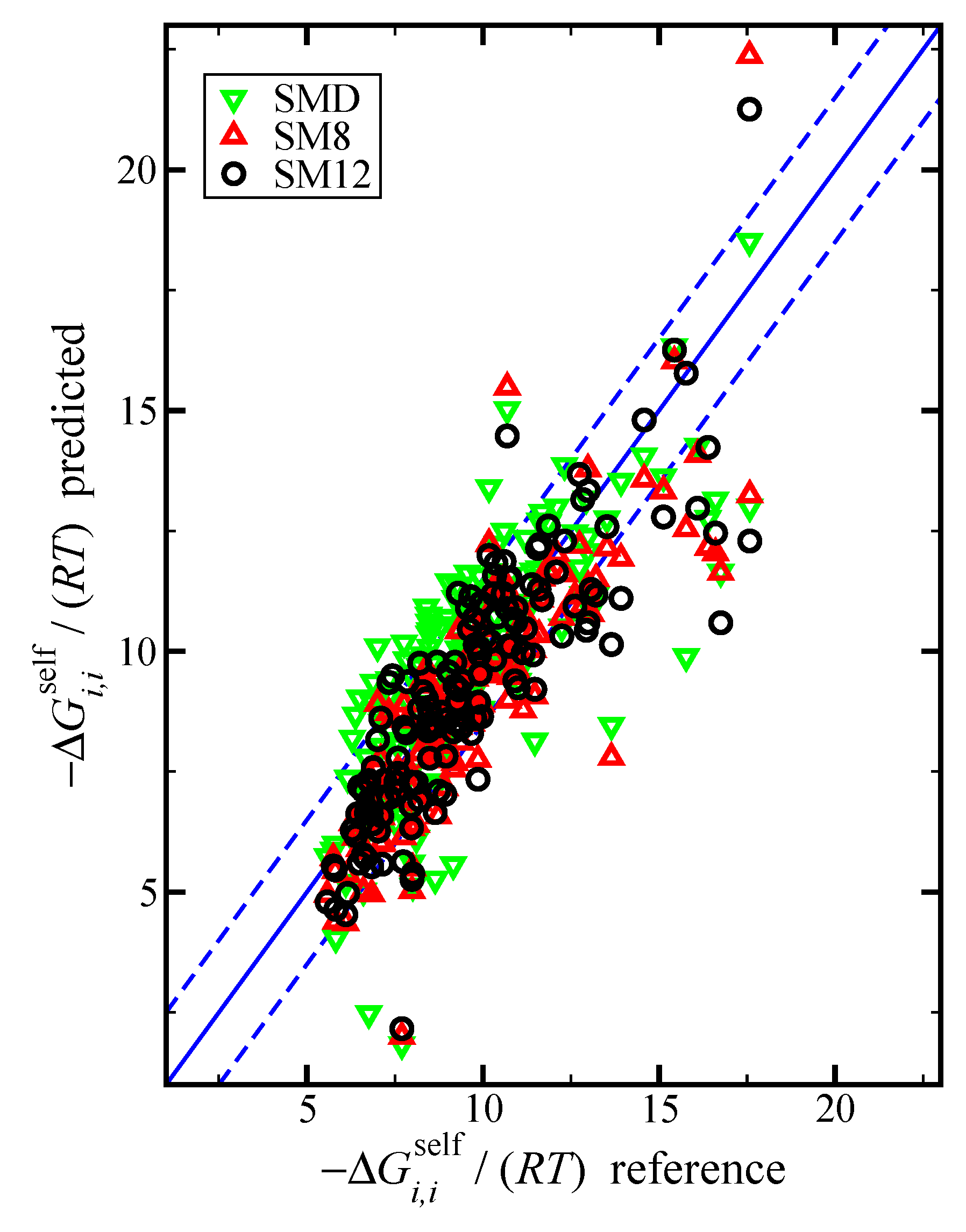
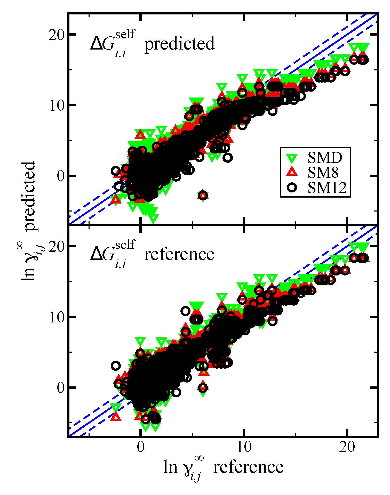
Figure 1.
Parity plot of the predicted versus reference values of the negative dimensionless self-solvation free energy, , using the SM12, SM8, and SMD universal solvent model, as indicated. The blue lines corresponds to the line, and the dashed blue lines correspond to and are drawn as a reference; the value of 1.5 was used based on the RMSE for the SM12 predictions.
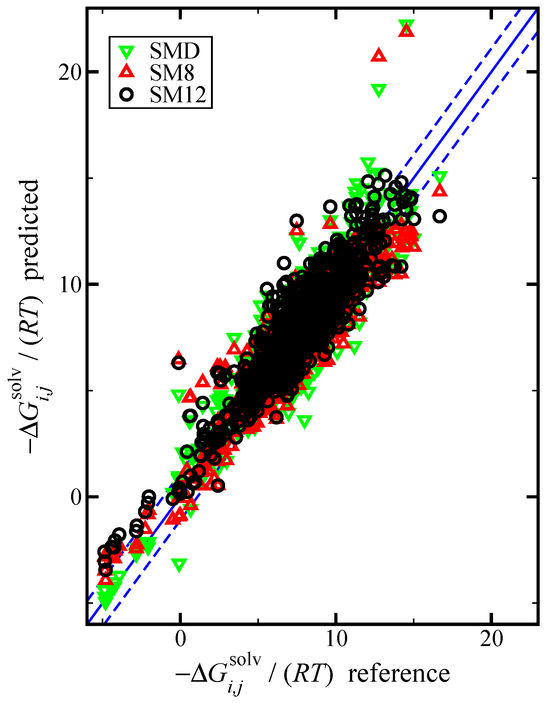
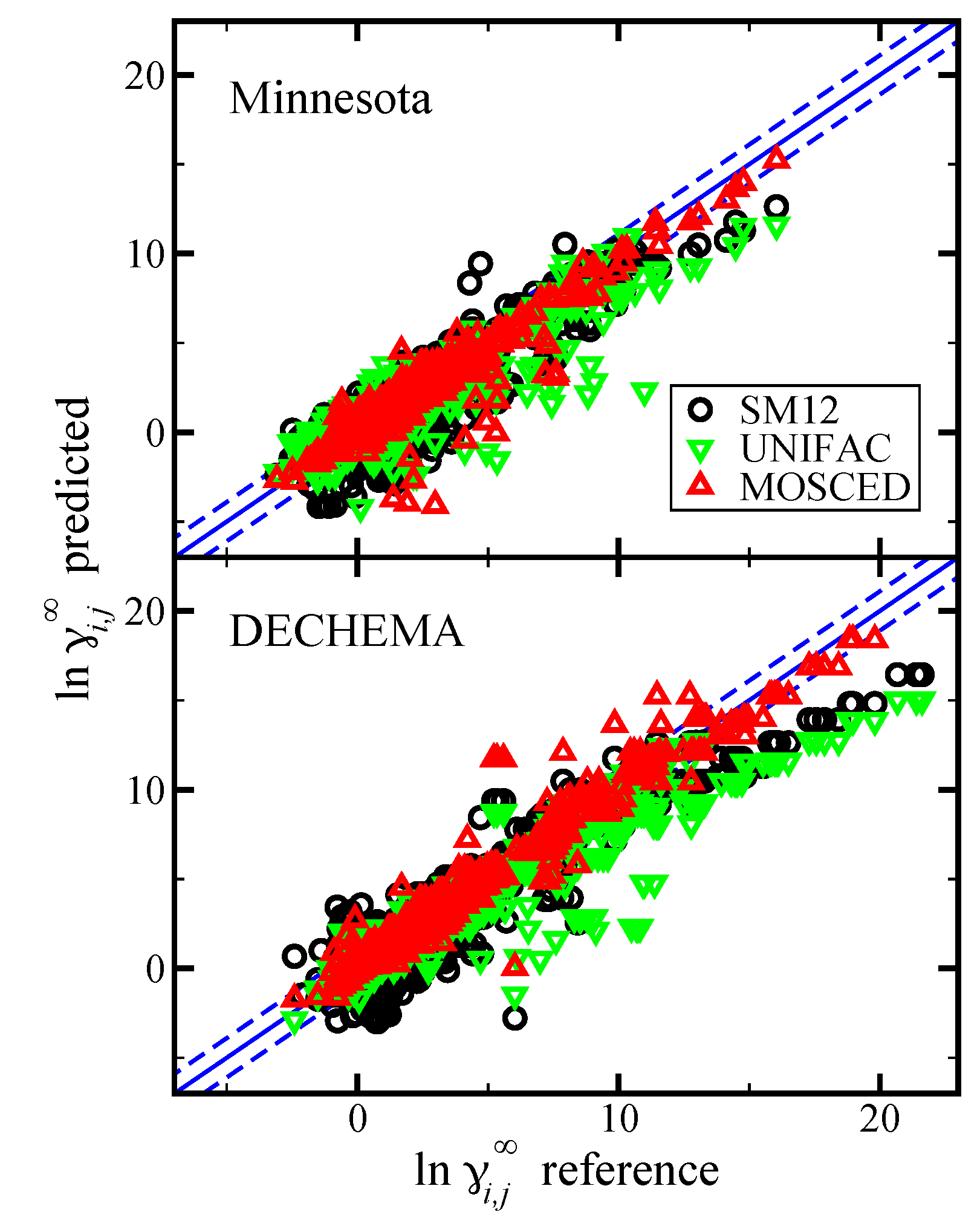
Figure 2.
Parity plot of the predicted versus reference values of the negative dimensionless solvation free energy, , using the SM12, SM8, and SMD universal solvent model, as indicated. The blue lines corresponds to the line, and the dashed blue lines correspond to and are drawn as a reference; the value of 1.1 was used based on the RMSE for the SM12 predictions. The reference values are from the Minnesota Solvation Database.
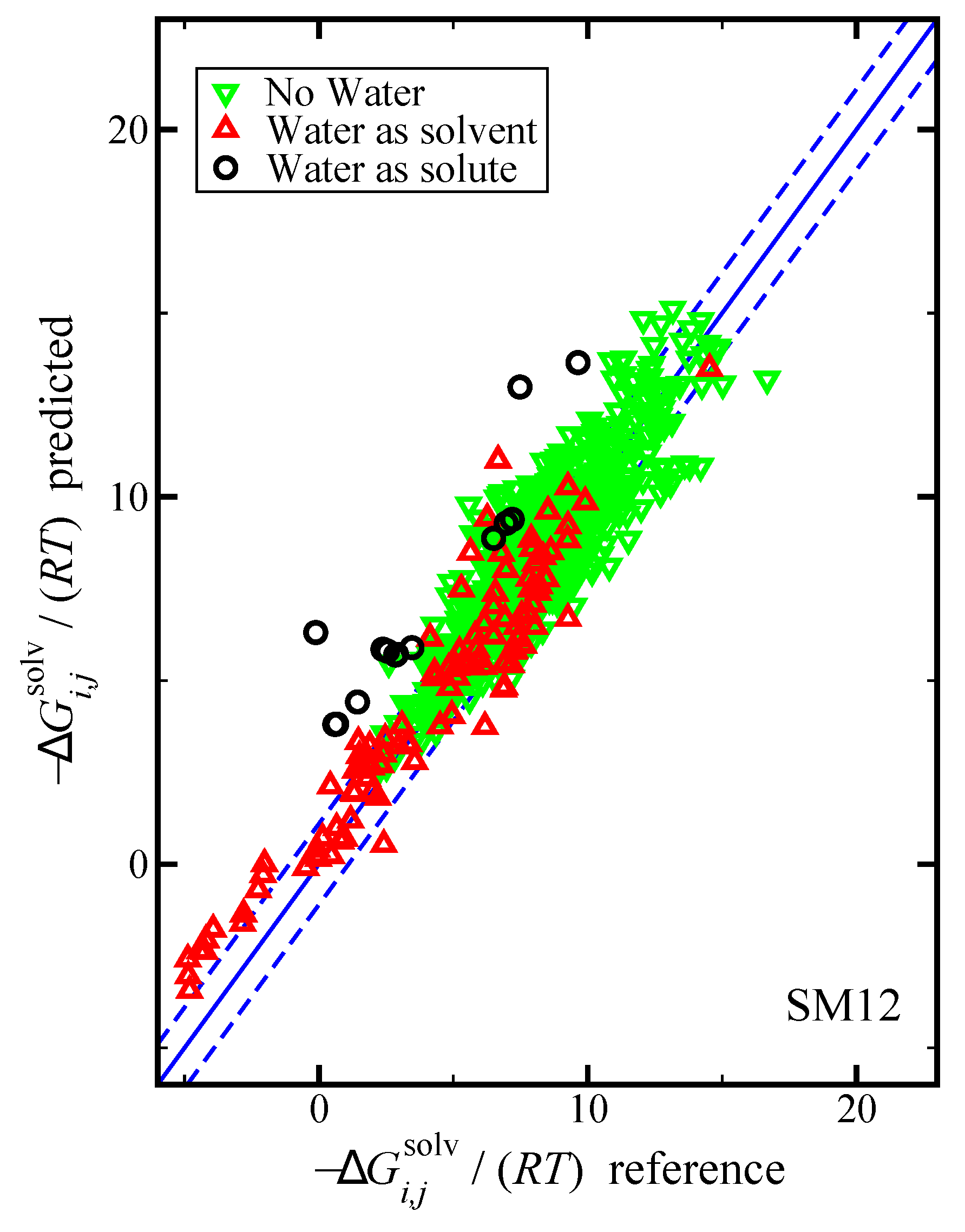
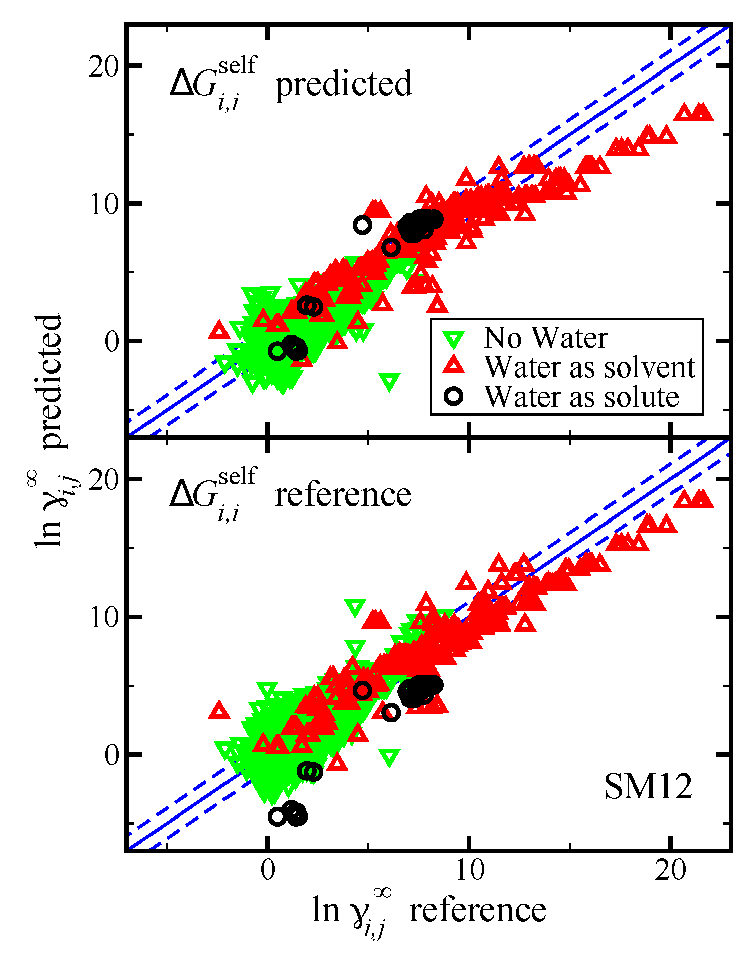
Figure 3.
Parity plot of the predicted versus reference values of using the SM12 universal solvent model for the case where water was the solvent, water was the solute, and where water was neither the solvent or solute, as indicated. The blue lines corresponds to the line, and the dashed blue lines correspond to and are drawn as a reference; the value of 1.1 was used based on the RMSE for the SM12 predictions. The reference values are from the Minnesota Solvation Database.
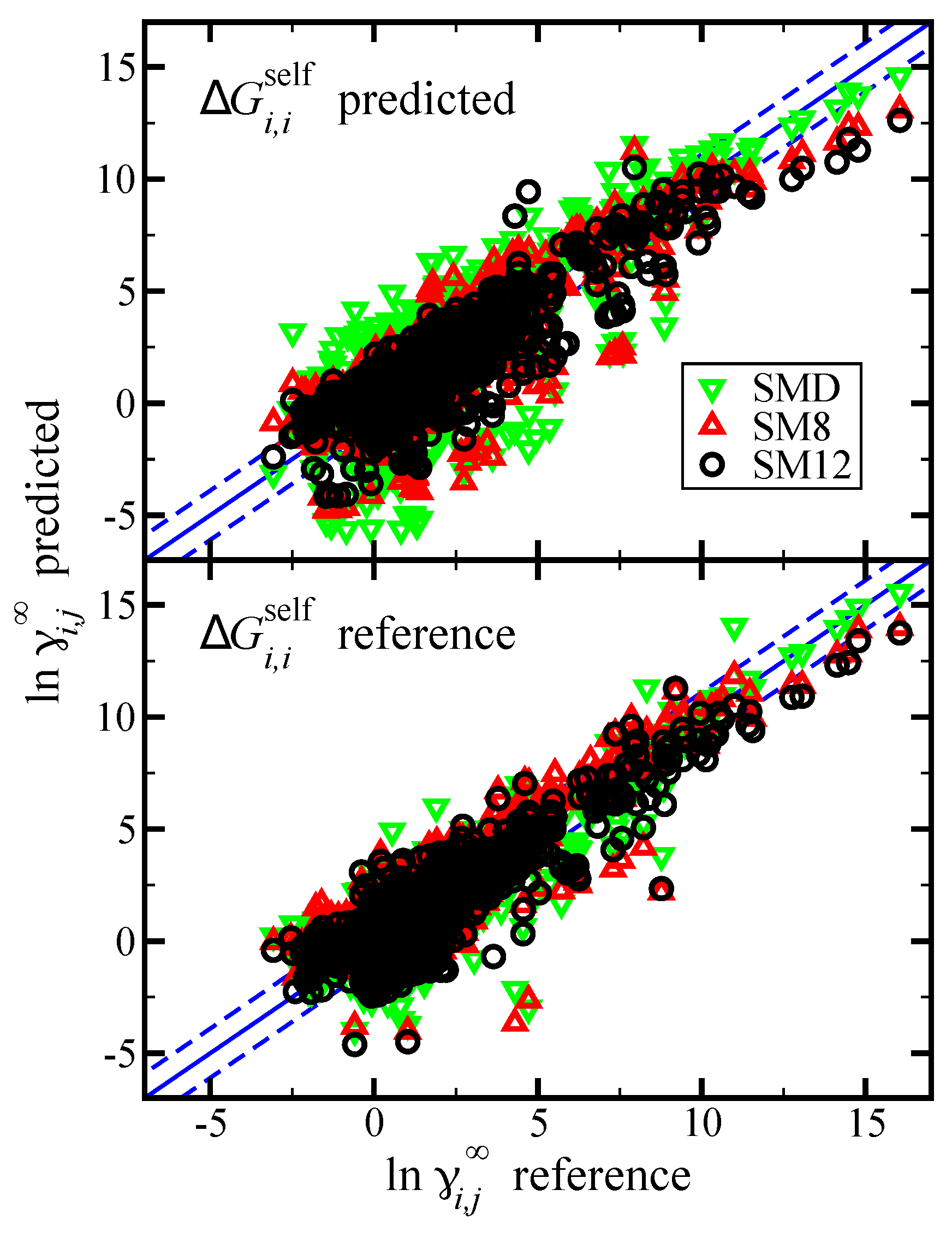
Figure 4.
Parity plot of the predicted versus reference values of
from the Minnesota Solvation Database version 2012 [
47]. Predictions are made using the SM12, SM8, and SMD universal solvent model, as indicated. The blue lines corresponds to the
line, and the dashed blue lines correspond to
and are drawn as a reference; the value of 1.1 was used based on the
RMSE for the SM12 predictions. In the top pane we present results when
was predicted using the SM12, SM8, or SMD universal solvent model. In the bottom pane we present results when
was computed using reference vapor pressure data.
Figure 5.
Parity plot of the predicted versus reference values of using the SM12 universal solvent model for the case where water was the solvent, water was the solute, and where water was neither the solvent or solute, as indicated. The blue lines corresponds to the line, and the dashed blue lines correspond to and are drawn as a reference; the value of 1.1 was used based on the RMSE for the SM12 predictions. The reference values are from the Minnesota Solvation Database. In the top pane we present results when was predicted using the SM12 universal solvent model. In the bottom pane we present results when was computed using reference vapor pressure data.
Figure 6.
Parity plot of the predicted versus reference values of from the DECHEMA. Predictions are made using the SM12, SM8, and SMD universal solvent model, as indicated. The blue lines corresponds to the line, and the dashed blue lines correspond to and are drawn as a reference. In the top pane we present results when was predicted using the SM12, SM8, or SMD universal solvent model. In the bottom pane we present results when was computed using reference vapor pressure data.
Figure 7.
Parity plot of the predicted versus reference values of using the SM12 universal solvent model for the case where water was the solvent, water was the solute, and where water was neither the solvent or solute, as indicated. The blue lines corresponds to the line, and the dashed blue lines correspond to and are drawn as a reference. The reference values are from DECHEMA. In the top pane we present results when was predicted using the SM12 universal solvent model. In the bottom pane we present results when was computed using reference vapor pressure data.
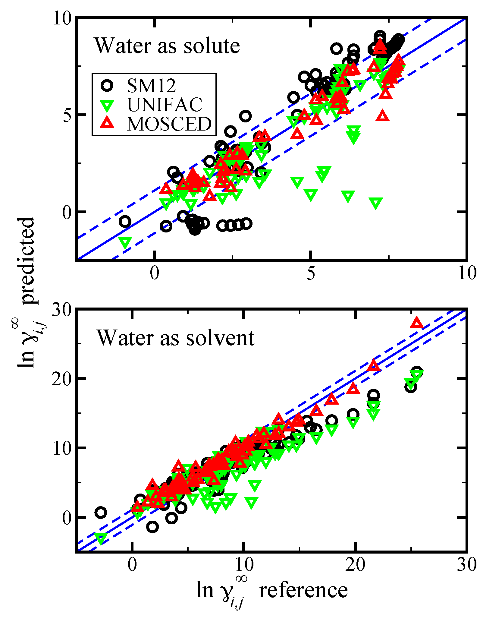
Figure 8.
Parity plot of the predicted versus reference values of
using the SM12 universal solvent model for the case where water was the solvent and water was the solute, as indicated. The blue lines corresponds to the
line, and the dashed blue lines correspond to
and are drawn as a reference. The reference values are from “Yaws’ Handbook of Properties for Aqueous Systems” [
56]. In the top pane we present results when
was predicted using the SM12 universal solvent model. In the bottom pane we present results when
was computed using reference vapor pressure data.
Figure 9.
Parity plot of the predicted versus reference values of
at 298.15 K using the SM12 universal solvent model, Universal Quasichemical Functional-group Activity Coefficients (UNIFAC), and modified separation of cohesive energy density (MOSCED) versus reference data from the Minnesota Solvation Database version 2012 (top pane) [
47] and DECHEMA (bottom pane) [
50,
51,
52,
53,
54,
55], as indicated. The blue lines corresponds to the
line, and the dashed blue lines correspond to
and are drawn as a reference. For the SM12 universal solvent model predictions,
was predicted.
Figure 10.
Parity plot of the predicted versus reference values of
at 298.15 K using the SM12 universal solvent model, UNIFAC, and MOSCED versus reference data from “Yaws’ Handbook of Properties for Aqueous Systems” [
56]. In the top pane results as shown for the case of water as the solute (water in organics), and in the bottom pane results are shown for the case of water as the solvent (organics in water). The blue lines corresponds to the
line, and the dashed blue lines correspond to
and are drawn as a reference. For the SM12 universal solvent model predictions,
was predicted.
Table 1.
A summary of the squared correlation coefficient (), root mean square error (RMSE), average absolute percent deviation (AAPD), and mean unsigned error (MUE) for the values of predicted using the SM12, SM8, and SMD universal solvent model as compared to the reference data.
Table 1.
A summary of the squared correlation coefficient (), root mean square error (RMSE), average absolute percent deviation (AAPD), and mean unsigned error (MUE) for the values of predicted using the SM12, SM8, and SMD universal solvent model as compared to the reference data.
| | |
|---|
| | SM12 | SM8 | SMD |
|---|
| 0.713 | 0.707 | 0.566 |
| RMSE | 1.526 | 1.600 | 1.820 |
| AAPD | 10.888 | 11.230 | 14.655 |
| MUE | 1.077 | 1.131 | 1.372 |
Table 2.
A summary of the squared correlation coefficient (), root mean square error (RMSE), average absolute percent deviation (AAPD), and mean unsigned error (MUE) for the values of predicted using the SM12, SM8, and SMD universal solvent model as compared to the reference data from the Minnesota Solvation Database.
| | |
|---|
| | SM12 | SM8 | SMD |
|---|
| 0.838 | 0.826 | 0.820 |
| RMSE | 1.120 | 1.125 | 1.181 |
| AAPD | 20.985 | 24.593 | 26.093 |
| MUE | 0.828 | 0.843 | 0.882 |
Table 3.
A summary of the squared correlation coefficient (), root mean square error (RMSE), and mean unsigned error (MUE) for , and the average absolute percent deviation (AAPD) for predicted using the SM12, SM8, and SMD universal solvent model as compared to the reference data from the Minnesota Solvation Database. For the predictions, we compare the case where (1) is predicted using the SM12, SM8, and SMD universal solvent model, and where (2) is computed using reference data, as indicated.
| | Predicted | Reference |
|---|
| | SM12 | SM8 | SMD | SM12 | SM8 | SMD |
|---|
| 0.796 | 0.740 | 0.627 | 0.806 | 0.796 | 0.788 |
| RMSE | 1.155 | 1.288 | 1.801 | 1.120 | 1.125 | 1.181 |
| AAPD | 89.856 | 107.821 | 357.706 | 92.482 | 134.797 | 131.626 |
| MUE | 0.840 | 0.883 | 1.376 | 0.828 | 0.842 | 0.882 |
Table 4.
A summary of the squared correlation coefficient (), root mean square error (RMSE), and mean unsigned error (MUE) for , and the average absolute percent deviation (AAPD) for predicted using the SM12, SM8, and SMD universal solvent model as compared to the reference data from DECHEMA. For the predictions, we compare the case where (1) is predicted using the SM12, SM8, and SMD universal solvent model, and where (2) is computed using reference data, as indicated.
| | Predicted | Reference |
|---|
| | SM12 | SM8 | SMD | SM12 | SM8 | SMD |
|---|
| 0.911 | 0.913 | 0.874 | 0.865 | 0.889 | 0.886 |
| RMSE | 1.163 | 1.065 | 1.382 | 1.354 | 1.196 | 1.271 |
| AAPD | 86.823 | 120.158 | 308.173 | 177.079 | 166.345 | 289.780 |
| MUE | 0.847 | 0.768 | 1.012 | 1.061 | 0.875 | 0.910 |
Table 5.
A summary of the squared correlation coefficient (
), root mean square error (
RMSE), and mean unsigned error (
MUE) for
, and the average absolute percent deviation (
AAPD) for
predicted using the SM12, SM8, and SMD universal solvent model as compared to the reference data from “Yaws’ Handbook of Properties for Aqueous Systems” [
56]. For the predictions, we compare the case where (1)
is predicted using the SM12, SM8, and SMD universal solvent model, and where (2)
is computed using reference data, as indicated. The results are additionally separated into case where water was the solvent and where water was the solute, as indicated.
| | Predicted | Reference |
|---|
| | SM12 | SM8 | SMD | SM12 | SM8 | SMD |
|---|
| | water as solute | water as solute |
| 0.889 | 0.793 | 0.645 | 0.889 | 0.793 | 0.645 |
| RMSE | 1.339 | 1.836 | 2.482 | 3.721 | 3.600 | 3.175 |
| AAPD | 168.491 | 645.592 | 2598.544 | 94.691 | 93.947 | 97.359 |
| MUE | 1.116 | 1.625 | 2.168 | 3.485 | 3.397 | 2.733 |
| | water as solvent | water as solvent |
| 0.913 | 0.928 | 0.907 | 0.916 | 0.946 | 0.951 |
| RMSE | 1.854 | 1.658 | 1.652 | 1.464 | 1.300 | 1.090 |
| AAPD | 117.058 | 160.651 | 327.313 | 409.655 | 197.774 | 176.344 |
| MUE | 1.353 | 1.191 | 1.317 | 1.115 | 1.017 | 0.792 |
Table 6.
A summary of the squared correlation coefficient (
), root mean square error (
RMSE), and mean unsigned error (
MUE) for
, and the average absolute percent deviation (
AAPD) for
predicted using UNIFAC and MOSCED as compared to the reference data from the Minnesota Solvation Database version 2012 [
47] and DECHEMA [
50,
51,
52,
53,
54,
55].
| | Minnesota | DECHEMA |
|---|
| | UNIFAC | MOSCED | UNIFAC | MOSCED |
|---|
| 0.820 | 0.884 | 0.915 | 0.976 |
| RMSE | 1.077 | 0.802 | 1.157 | 0.524 |
| AAPD | 52.595 | 41.251 | 41.044 | 131.758 |
| MUE | 0.634 | 0.422 | 0.559 | 0.241 |
Table 7.
A summary of the squared correlation coefficient (
), root mean square error (
RMSE), and mean unsigned error (
MUE) for
, and the average absolute percent deviation (
AAPD) for
predicted using UNIFAC and MOSCED as compared to the reference data from “Yaws’ Handbook of Properties for Aqueous Systems” [
56]. The results are separated for the case of water as the solute (water in organics) and water as the solvent (organics in water).
| | Water As Solute | Water As Solvent |
|---|
| | UNIFAC | MOSCED | UNIFAC | MOSCED |
|---|
| 0.713 | 0.923 | 0.816 | 0.962 |
| RMSE | 1.423 | 0.688 | 2.479 | 1.000 |
| AAPD | 51.395 | 55.749 | 77.925 | 138.245 |
| MUE | 0.824 | 0.532 | 1.647 | 0.761 |


