Extreme Learning Machine-Based Model for Solubility Estimation of Hydrocarbon Gases in Electrolyte Solutions

Abstract

Calculating hydrocarbon components solubility of natural gases is known as one of the important issues for operational works in petroleum and chemical engineering. In this work, a novel solubility estimation tool has been proposed for hydrocarbon gases—including methane, ethane, propane, and butane—in aqueous electrolyte solutions based on extreme learning machine (ELM) algorithm. Comparing the ELM outputs with a comprehensive real databank which has 1175 solubility points yielded R-squared values of 0.985 and 0.987 for training and testing phases respectively. Furthermore, the visual comparison of estimated and actual hydrocarbon solubility led to confirm the ability of proposed solubility model. Additionally, sensitivity analysis has been employed on the input variables of model to identify their impacts on hydrocarbon solubility. Such a comprehensive and reliable study can help engineers and scientists to successfully determine the important thermodynamic properties, which are key factors in optimizing and designing different industrial units such as refineries and petrochemical plants.

1. Introduction

Solubility of hydrocarbon and nonhydrocarbon gases—i.e., mixtures of methane, ethane, propane, CO₂, and N₂ in aqueous phases—is known as one of the important practical and theoretical challenges in petroleum, geochemical, and chemical engineering. This property has an effective role in different processes, such as achieving optimum conditions for oil and gas transportation, gas hydrate formation, designing thermal separation processes, gas sequestration for protecting environment, and coal gasification. Petroleum reservoirs normally have some natural gases with aqueous solution at high-pressure and high-temperature conditions so that the solubility of gas becomes attractive for engineers [1,2,3,4,5,6,7,8]. In production and transportation of hydrocarbons, it is possible that water content of gas undergoes an alteration in phase from vapor to ice and gas hydrates. The crystalline solid phases called gas hydrates are created when small-sized gas molecules are trapped in lattice of water molecules. Creation of hydrates can cause major flow assurance problems during production and transportation of hydrocarbons steps such as pipeline blockage, corrosion, and many other issues resulted from the two-phase flow [1,9,10,11].

In the recent years, investigations on CO₂ solubility in aqueous electrolyte solutions have grown significantly as well as they are related to CO₂ capture and storage. It is a clear fact that the dominant cause of global warming is emission of CO₂ gas generated from fossil fuels so its sequestration and disposal in the ocean have been known as a reasonable choice to overcome global warming problems [12,13,14]. Simulation of enhanced oil recovery, design of supercritical extraction, and optimization of CO₂ dissolution in the ocean need a comprehensive knowledge about carbon dioxide solubility in aqueous electrolytes solutions [13,14,15].

Investigation of natural gas phase behavior in aqueous solutions in different operational conditions is known one of the important issues in the industry, which has wide applications for avoiding problems in designing and optimization of gas processing. In the literature, there are different solubility datasets for various gas–liquid systems. These datasets mostly include hydrocarbons’ dissolution in water/brine systems [1,4,5,9,16,17,18,19,20] and non-hydrocarbons such as CO₂ and N₂ dissolution in water/brine systems [7,12,13,14,18,21,22,23,24]. A brief summary of the hydrocarbon systems datasets is shown in

Table 1. Details of experimental hydrocarbons solubility in aqueous electrolyte solutions.

Author	P (Mpa)	T (°C)	Composition	Mole Fraction of the Components in the Gaseous Phase
Culberson et al.	0.8–69.61	37.78–171.11	Pure water	C1: 0.0000698–0.0033
Kiepe et al.	0.304–10.23	40–100.14	Pure water, LiBr, KBr, LiCl, KCl	C1: 0.00003–0.00154
Chapoy et al.	0.357–18	1.98–95.01	Pure water	C1: 0.000204–0.002459
				C2: 0.0000147–0.0000674
				C3: 0.0000321–0.0002694
				C4: 0.00000387–0.00001121
Marinakis et al.	6.22–20.1	1.4–25.98	Pure water, NaCl	C1: 0.00099–0.00282
				C2: 0.000038–0.000249
				C3: 0.000006–0.000042
Crovetto et al.	1.327–6.451	24.35–245.15	Pure water	C1: 0.0002124–0.0010337
Wang et al.	1–40.03	2.5–30.05	Pure water	C1: 0.000563–0.004049
				C2: 0.0000986–0.000864
Amirjafari	4.66–56.16	54.44–104.44	Pure water	C1: 0.00045–0.0037
				C2: 0.000119–0.001768
				C3: 1.9 × 10−5–0.001863
O’Sullivan et al.	10.2–62	51.5–125	Pure water, NaCl	C1: 0.000805–0.0043
				C2: 0.000825–0.001438
Michels et al.	4.09–45.89	25–150	Pure water, NaCl, LiCl, NaBr, NaI, CaCl2	C1: 0.000173–0.00269
Mohammadi et al.	1.14–31.1	4.65–24.75	Pure water	C1: 0.000313–0.00311
Vul’fson et al.	2.53–60.8	19.95–79.95	Pure water	C1: 0.000361–0.004328
Dhima	2.5–100	71	Pure water	C1: 0.000127–0.005085
				C2: 0.000821–0.001398
				C4: 0.000021–0.000103

for hydrocarbons. The experimental data of water content of hydrocarbons and non-hydrocarbons are limited because of difficulties in measurement of the low water content gases at high pressure and low temperature. Mohammadi and coworkers expressed that an accurate estimation of water content can be obtained by gas solubility data, therefore, they overcame the complexities of experimental determination of the water content in natural gases [1]. Due to limited number of measurement data, wide attempts have been made to model and describe the gas-liquid equilibrium in aqueous electrolyte solutions. There are several thermodynamic models which uses the Henry’s constant, activity coefficient, and cubic equations of state to obtain more information about the equilibrium conditions. The changes of Henry’s constant for the pressure lower than 5 MPa are negligible and it is dominantly affected by temperatures [19]. The high dependency on temperature is obvious at low temperature and also the nonlinear decreasing relationship is observed at high temperatures [25]. Furthermore, there is just a limited number of Henry’s constants for hydrocarbon systems at low temperature. According to this fact, there are several drawbacks in applying the Henry’s law, whereas it has great ability for accurate prediction of solubility. As an example, it is suitable for dilute solutions or near-ideal solutions [26]. Additionally, this method is correct for single compounds in no chemical reaction conditions for aqueous phase. Another method is cubic EOS which has several advantages such as small number of parameters, computational efficiency, and ease of performance [3,4,21]. The EOSs were proposed originally for pure fluids, after that, their applications were expanded for mixtures by combining the constants from different pure components. This extension can be done by different methods such as Dalton’s law of additive partial pressures and Amagat’s rule of additive volumes [5]. For complex compounds, there are some limitations in accuracy of EOS which highlight the importance of empirical adjustments by dealing with the binary interaction parameters. In order to determine these parameters, a reliable source of experimental data for vapor-liquid equilibrium is required which induces some uncertainty into EOSs [7].

Due to above discussions, development of an accurate and reliable approach for estimation of solubility of hydrocarbons and non-hydrocarbons in aqueous electrolyte solutions has been highlighted. Nowadays, machine learning approaches have shown extensive applications in different topics [27,28,29,30,31,32,33,34,35]. This work organizes a novel artificial intelligence method called extreme learning machine (ELM) to estimate solubility of hydrocarbons in aqueous electrolyte mixtures in terms of types of gas, mole fractions of gases, pressure, temperature, and ionic strength.

2. Methodology

2.1. Experimental Dataset Collection

In order to construct a highly accurate and comprehensive model capable of estimating the solubility of mixtures of hydrocarbons in aqueous electrolyte solutions, a comprehensive databank was provided based on existing experimental data in Table 1. This databank contains total number of 1175 solubility points for hydrocarbons (881 and 294 points for training and testing phases, respectively) (see Table S1 of data set in Supplementary Materials). According to the literature [1,4,5,9,16,17,18,19,20], the solubility of gases in these systems is highly function of aqueous solutions, pressure, temperature, and gaseous phase composition. The aqueous phase composition was change into ionic strength (I) from salt concentrations to reduce dimensions of modeling process. The following equation presents the relationships between ionic strength, valance of charged ions (z_i), and molar concentration of each ion (m_i).

$$I=\frac{1}{2}\sum m_i{\left|z_i\right|}^2$$

(1)

In this study, the solubility of hydrocarbons is predicted in terms of concentration of components in gaseous mixture, ionic strength of solution, temperature, and pressure.

$${\eta }_h=f\left(C1,C2,C3,C4,I,P,T,idx\right)$$

(2)

In which, ${\eta }_h$ represents the hydrocarbon solubility in aqueous phase; C(1–4) are known as the methane, ethane, propane, and butane mole fraction in gas phase (0–99.99); I denotes the ionic strength based on molarity (0–37.35); T denotes the temperature in terms of °C (1.4–245.15); P shows the pressure in MPa (0.3–100), and idx symbolizes the index of fraction whose solubility is to be determined (1,2,3,4).

2.2. Extreme Learning Machine

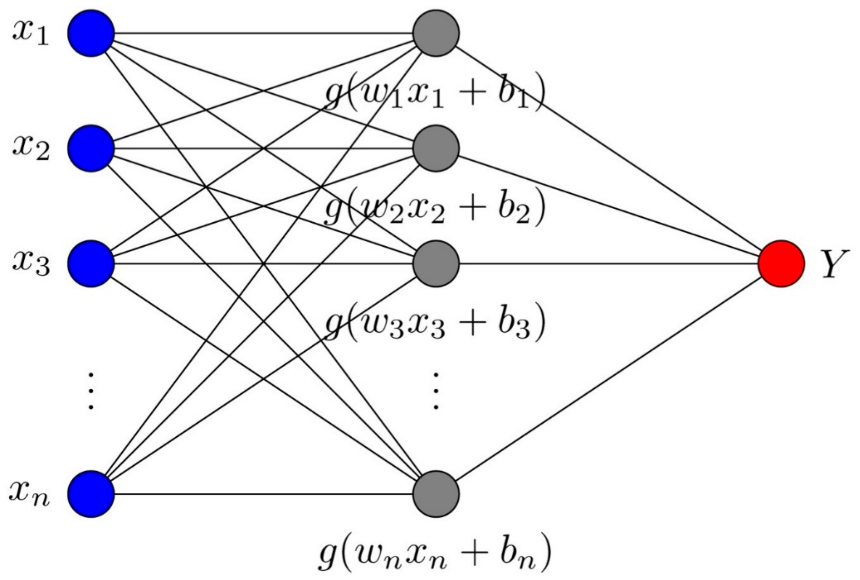
Huang proposed a new intelligence method based on single-layer feedforward neural network (SLFFNN) called extreme learning machine to satisfy the drawbacks of gradient-based algorithms such low training speed and low learning rate. In the ELM algorithm, the hidden nodes are selected randomly and the weights of output of the SLFFNN are calculated by applying Moore–Penrose generalized inverse [36,37].

The scheme of ELM algorithm is demonstrated in Figure 1. By assuming N training sets such as (x_i, y_i) ∈ Rⁿ × R^m for L hidden nodes, the SLFFNN algorithms can be written as

$${{\displaystyle \sum }}_{i=1}^L{\beta }_i{f}_i\left(x_j\right)={{\displaystyle \sum }}_{i=1}^L{\beta }_i{f}_i\left(a_i.b_i.x\right) j=1, \dots , N$$

(3)

In which, a_i = [a_i1, …, a_in]^T points to input weights matrix which is related to hidden nodes, β_i = [β_i1, …, β_im]^T represents the output weights matrix which is related to hidden nodes, and b_i symbolizes the hidden layer bias.

$${{\displaystyle \sum }}_{i=1}^L{\beta }_i{f}_i\left(x_j\right)=H\beta$$

(4)

In which, β = [β₁, …, β_L] and h(x) = [h₁(x), …h_L(x)] are known as the hidden layer output matrix and the output weight matrix.

The first step of this model is the random calculation of input weight and the bias of hidden layer for the training phase. Then, for determining these values, the hidden layer matrix is obtained by utilization of input variables. Then, the SLFFNN training is changed to a least-square problem. The ELM algorithms implement regularization theory to define a target function as [38,39,40]

$$\min L_{ELM}=\frac{1}{2}{\left|\left|\beta \right|\right|}^2+\frac{c}{2}{\left|\left|T-H\beta \right|\right|}^2$$

(5)

3. Results and Discussion

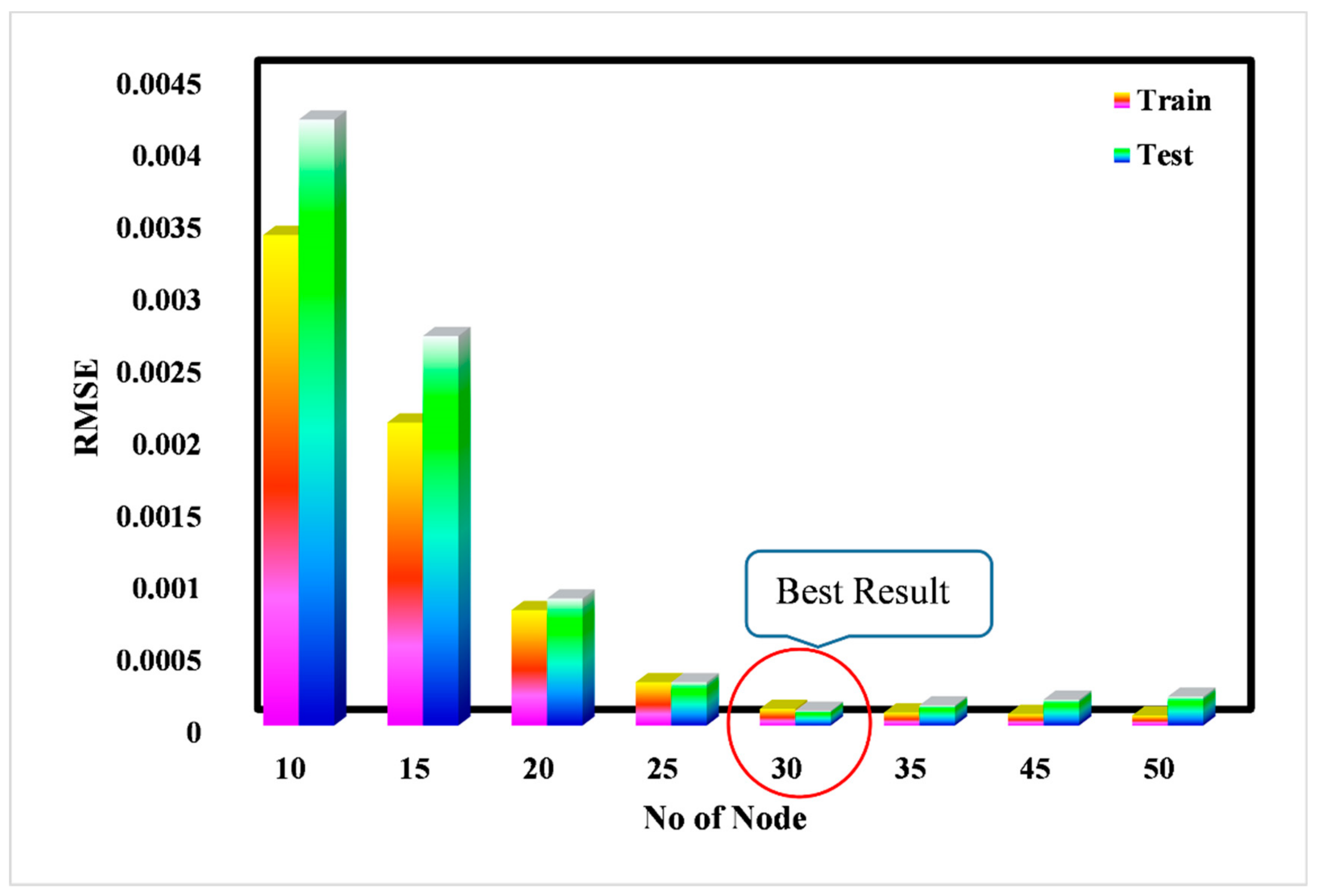
In this study, the solubility of hydrocarbons in the aqueous electrolyte phase is determined based on ELM algorithm. To this end, the sigmoid function is set as activation function and the input weights were initialized randomly in range of (−1, 1). Additionally, the number of nodes in the hidden layers was estimated as 30 based on the lowest value of RMSE as determined in Figure 2. As shown, after 30 nodes, by increasing complexity of model, the testing error increased so the optimum structure of the algorithm has 30 nodes to prohibit overfitting.

In the following, the statistical results of the estimation of hydrocarbon solubility are inserted in

Table 2. Statistical analyses of developed model.

Dataset	R2	MRE (%)	MSE	RMSE
Training	0.985	22.049	1.33285 × 10−8	0.0001
Testing	0.987	22.054	1.05351 × 10−8	0.0001
Overall	0.985	22.050	1.26295 × 10−8	0.0001

. The following equations are used to achieve this end:

$$\mathrm{Mean} \mathrm{relative} \mathrm{error} \left(\mathrm{MRE}\right) =\frac{100}{N}{{\displaystyle \sum }}_{i=1}^N(\frac{X_i^{actual}-X_i^{predicted}}{X_i^{actual}})$$

(6)

$$\mathrm{Root} \mathrm{mean} \mathrm{square} \mathrm{error} \left(\mathrm{RMSE}\right) =\sqrt{\frac{1}{N}{{\displaystyle \sum }}_{i=1}^N({\left(X_i^{actual}-X_i^{predicted}\right)}^2)}$$

(7)

$$\mathrm{Mean} \mathrm{squared} \mathrm{error} \left(\mathrm{MSE}\right) = \frac{1}{N}{\displaystyle \sum }_{i=1}^N{\left(X_i^{actual}-X_i^{predicted}\right)}^2$$

(8)

$$\mathrm{R}-\mathrm{squared} (\mathrm{R}2) =1-\frac{{{\displaystyle \sum }}_{i=1}^N{\left(X_i^{actual}-X_i^{predicted}\right)}^2}{{{\displaystyle \sum }}_{i=1}^N{\left(X_i^{actual}-\overline{X^{actual}}\right)}^2}$$

(9)

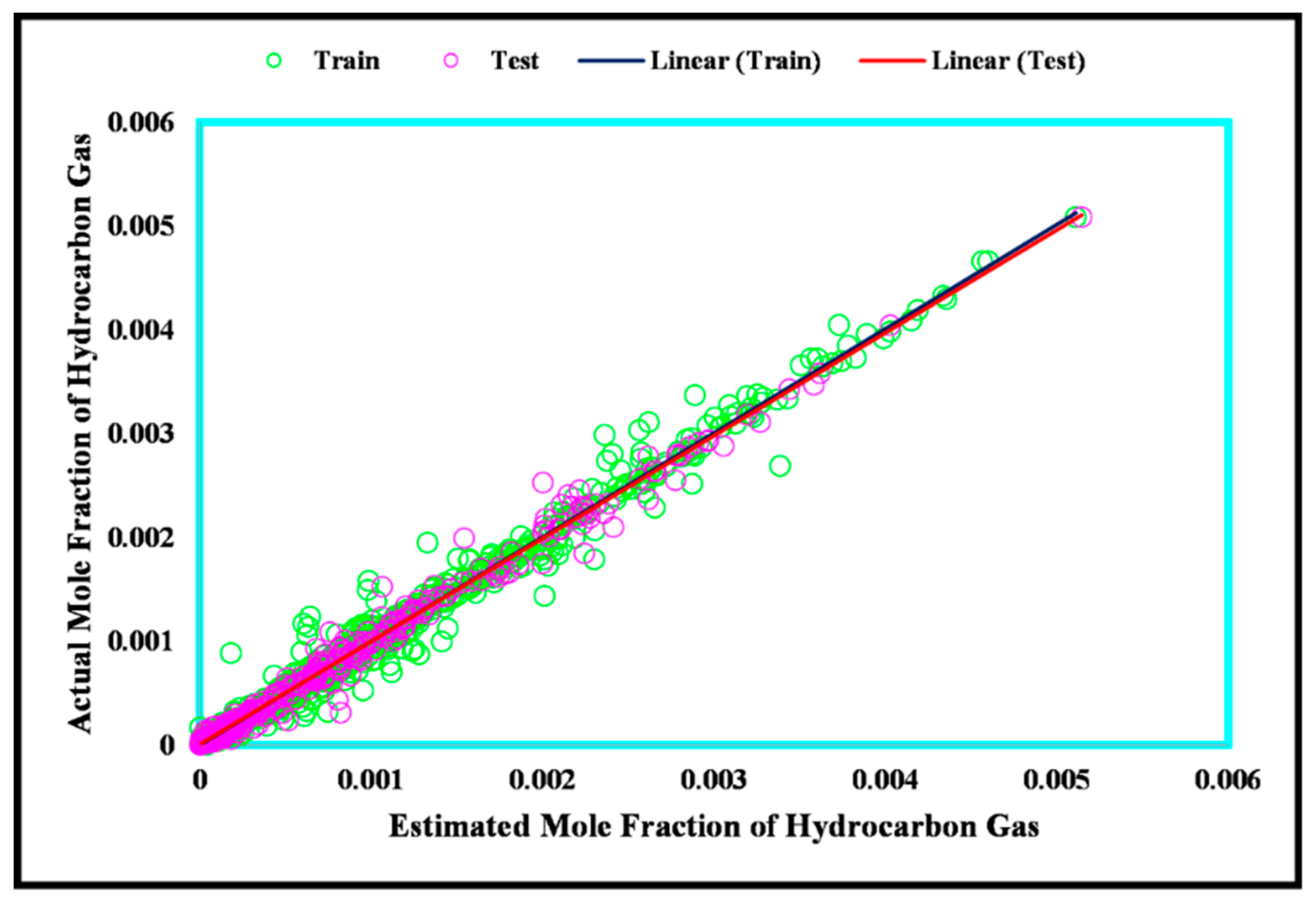
As shown in Table 2, the MRE, MSE, and RMSE are determined as 22.049, 1.33285 × 10⁻⁸, and 0.0001 for training phase respectively. Moreover, for testing phase, MRE = 22.054, MSE = 1.05351 × 10⁻⁸ and RMSE = 0.0001 are calculated. The estimated R² values are 0.985, 0.987, and 0.985 for training, testing, and overall datasets respectively. These results give the knowledge about the high degree of accuracy for proposed ELM algorithm.

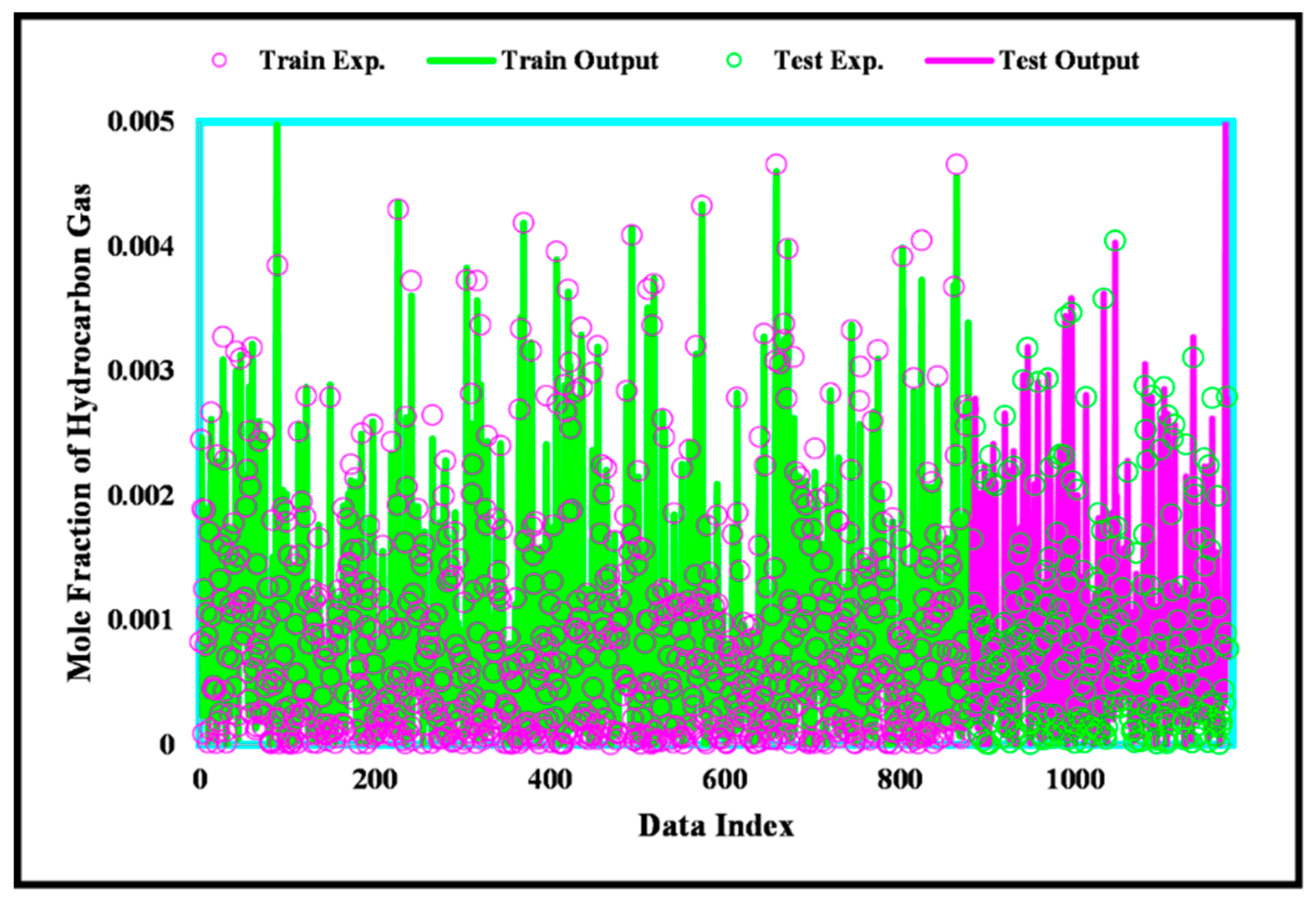
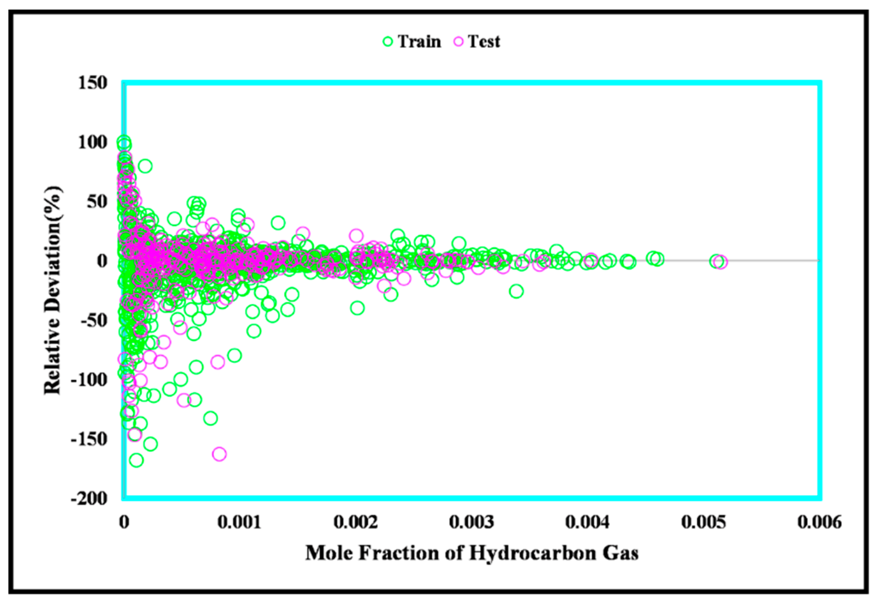
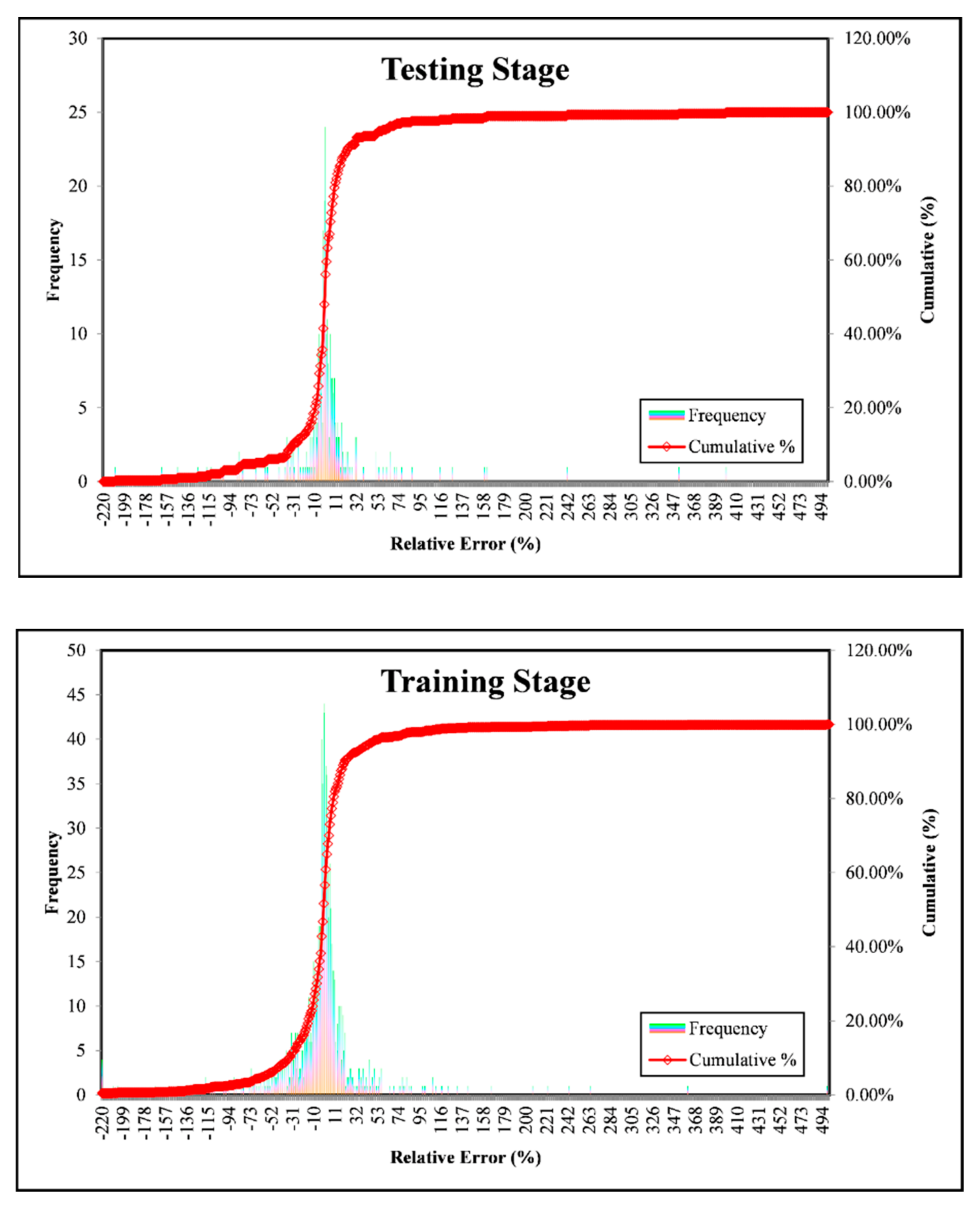
On the one hand, the comparison between the estimated and real hydrocarbons solubility in aqueous electrolyte solutions are shown in Figure 3. This depiction demonstrates an excellent agreement between estimated and real solubility values. Figure 4 also represents the regression plot of actual hydrocarbons solubility versus estimated one. A light cloud of data near the 45° line expresses the validity and accuracy of ELM algorithm. Additionally, Figure 5 also shows the distribution of relative deviations between forecasted and actual hydrocarbons solubility in aqueous solutions. It can be seen that the ELM outputs deviate slightly from the real solubility and most of relative deviations are near to zero. Furthermore, Figure 6 shows the histograms of relative deviations for training and testing phases. In this demonstration, frequency diagram confirms that most of the error points are close to zero and also cumulative axis express the fact that range of deviation is very limited and the highest slope of the cumulative curve occurred near the zero point.

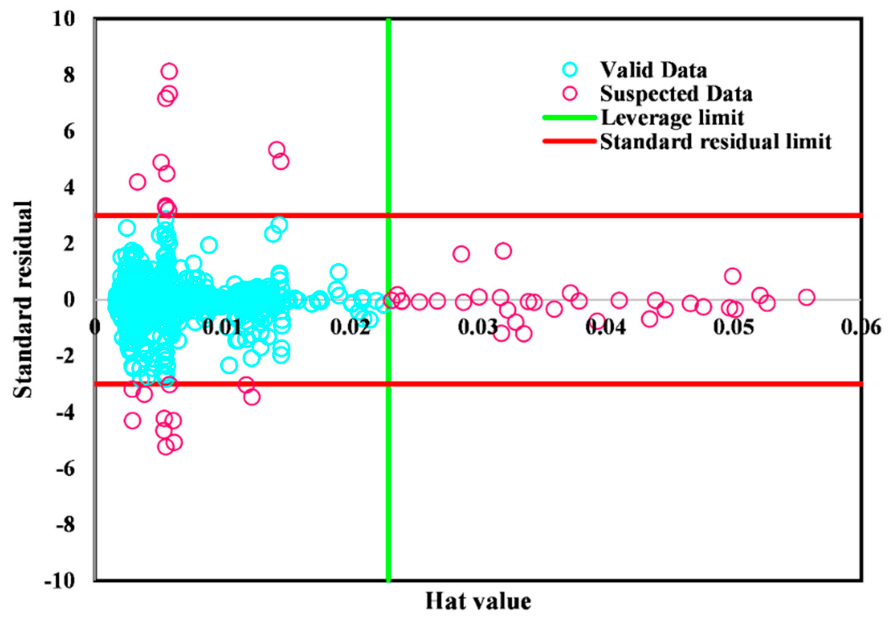
The ELM algorithm implemented in the current work shows an excellent ability in calculation of solubility of hydrocarbons in aqueous phases. One of the important factors which can influence the validation of model is degree of precision of utilized data. In order to clarify the accuracy of solubility databank, the leverage mathematical method is recruited. This method has some rules to identify the suspected solubility data so that a matrix which is known as hat matrix, should be constructed based on formulation [41,42,43,44,45]

$$H=U{\left(U^{T}U\right)}^{-1}{U}^T$$

(10)

In which, U symbolizes a matrix of i × j dimensional. i and j are known as the number of algorithm parameter and training points which are used for determination of critical leverage limit as

$$H^{*}=3\left(j+1\right)/i$$

(11)

In order to detect the reliable zone, there are two standard residual indexes (−3 and 3) which are used in the leverage method. As shown in Figure 7, the reliable area is bound by these two residual indexes and critical leverage limit. The critical straight lines are shown by red and green colors. This plot is known as William’s plot. In this plot, normalized residual is depicted versus hat value which is determined from the main diagonal of aforementioned matrix. It is obvious that the major number of solubility data are located in this area which expresses validation of the hydrocarbon solubility databank.

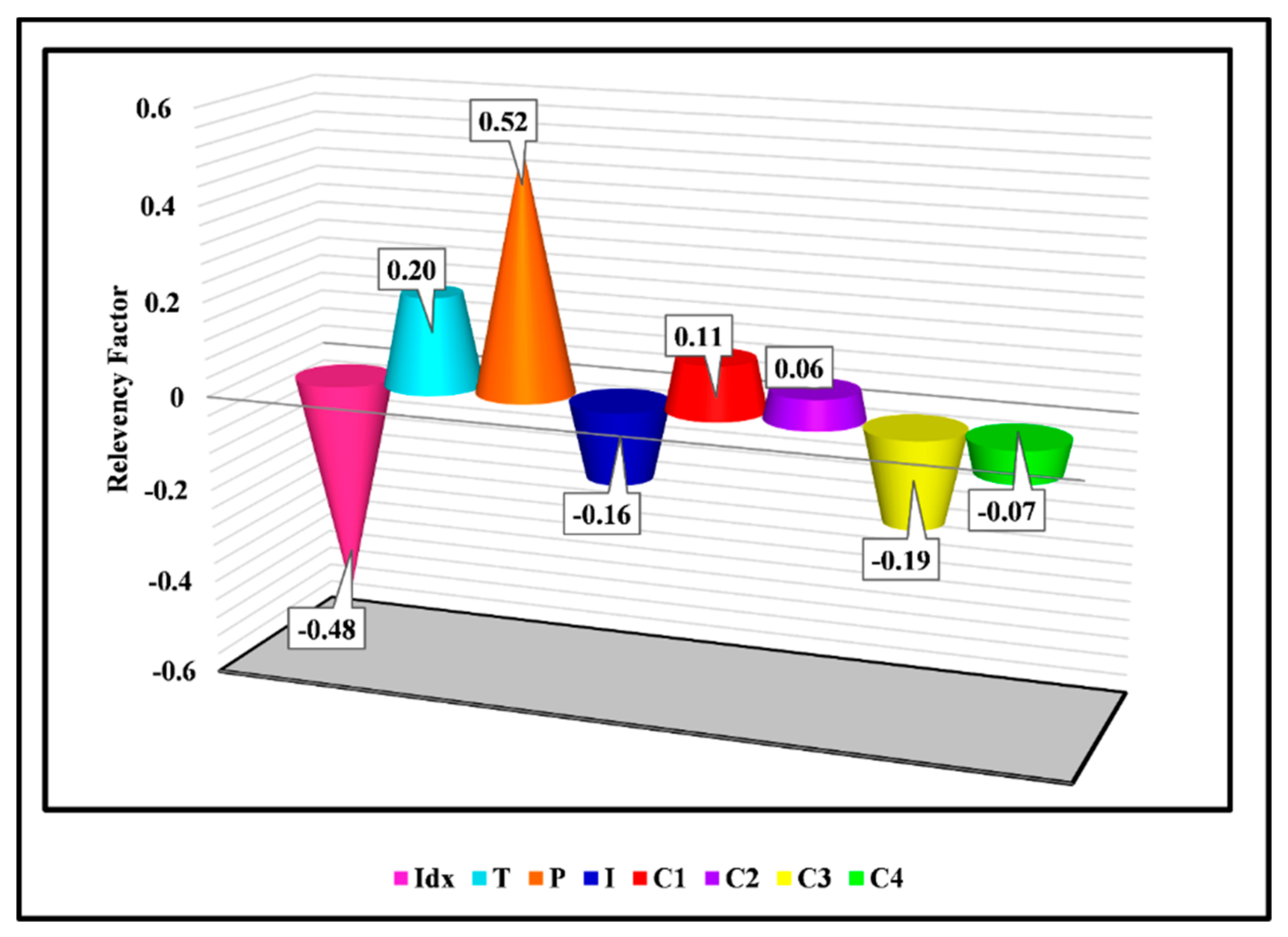
In the most of parametric studies, it is a valuable attempt to identify the effectiveness of all inputs on the target. According to this fact, the sensitivity analysis is employed to investigate effect of concentration of components in gaseous mixture; ionic strength of solution; and temperature and pressure on the solubility of hydrocarbons in aqueous electrolyte systems. To this end, the relevancy factor should be determined as follows for each input parameter [46,47,48,49,50,51,52,53,54]:

$$r=\frac{{{\displaystyle \sum }}_{i=1}^n(X_{k,i}-\overline{X_k})\left(Y_i-\overline{Y}\right)}{\sqrt{{{\displaystyle \sum }}_{i=1}^n{(X_{k,i}-\overline{X_k})}^2{{\displaystyle \sum }}_{i=1}^n(Y_i-{\overline{Y)}}^2}}$$

(12)

In which $Y_i$ and $\overline{Y}$ denote the ‘i’ th output and output average. $X_{k,i}$ and $\overline{X_k}$ are known as ‘k’ th of input and average of input. Figure 8 shows the relevancy factor for each effective variable of hydrocarbon solubility. It is necessary to explain that the relevancy factor lies in range of −1 to 1 so that the higher absolute value has more impact on hydrocarbon solubility. Furthermore, the positive relevancy factor shows the straight relationship between input and target. The relevancy factors for pressure, temperature, the index of fraction, ionic strength, methane, ethane, propane, and butane mole fraction in gas phase are 0.52, 0.20, −0.48, −0.16, 0.11, 0.06, −0.19, and −0.07 respectively. According to this explanation and results, as pressure, temperature, and mole fraction of methane and ethane increase, the solubility of investigated hydrocarbon increases. Moreover, pressure and mole fraction of ethane in gaseous phase are the most and least effective parameters for determination of solubility of hydrocarbons.

4. Conclusions

The hydrocarbon solubility in aqueous electrolyte phases at high temperature and pressure conditions is known as a major effective parameter in variety of applications for petroleum industries and chemical engineering. Numerous attempts have been made in the current study to suggest a highly accurate and comprehensive predicting tool on the basis of extreme learning machine to calculate hydrocarbons solubility in wide ranges of operational conditions. Comparing the ELM outputs with a comprehensive real databank which has 1175 solubility points concluded to R-squared values of 0.985 and 0.987 for training and testing phases respectively. The excellent agreements of ELM and real hydrocarbon solubility values express that the ELM algorithm is a valuable tool for design and optimization of various processes that are related to vapor-liquid equilibrium. Furthermore, this study gives more information about the intensity of each input parameter on solubility of hydrocarbons. Due to the aforementioned results, this work has potential application in commercial software packages such as CMG and ECLIPSE for simulation of fluid flow in porous media.

References

- Mohammadi, A.H.; Chapoy, A.; Tohidi, B.; Richon, D. Gas solubility: A key to estimating the water content of natural gases. Ind. Eng. Chem. Res. 2006, 45, 4825–4829. [Google Scholar] [CrossRef]
- Chapoy, A.; Haghighi, H.; Tohidi, B. Development of a Henry’s constant correlation and solubility measurements of n-pentane, i-pentane, cyclopentane, n-hexane, and toluene in water. J. Chem. Thermodyn. 2008, 40, 1030–1037. [Google Scholar] [CrossRef]
- Chapoy, A.; Mokraoui, S.; Valtz, A.; Richon, D.; Mohammadi, A.H.; Tohidi, B. Solubility measurement and modeling for the system propane–water from 277.62 to 368.16 K. Fluid Phase Equilibria 2004, 226, 213–220. [Google Scholar] [CrossRef]
- Chapoy, A.; Mohammadi, A.H.; Richon, D.; Tohidi, B. Gas solubility measurement and modeling for methane–water and methane–ethane–n-butane–water systems at low temperature conditions. Fluid Phase Equilibria 2004, 220, 111–119. [Google Scholar] [CrossRef]
- Dhima, A.; de Hemptinne, J.-C.; Moracchini, G. Solubility of light hydrocarbons and their mixtures in pure water under high pressure. Fluid Phase Equilibria 1998, 145, 129–150. [Google Scholar] [CrossRef]
- Kiepe, J.; Horstmann, S.; Fischer, K.; Gmehling, J. Experimental determination and prediction of gas solubility data for methane+ water solutions containing different monovalent electrolytes. Ind. Eng. Chem. Res. 2003, 42, 5392–5398. [Google Scholar] [CrossRef]
- Bamberger, A.; Sieder, G.; Maurer, G. High-pressure (vapor+ liquid) equilibrium in binary mixtures of (carbon dioxide+ water or acetic acid) at temperatures from 313 to 353 K. J. Supercrit. Fluids 2000, 17, 97–110. [Google Scholar] [CrossRef]
- Mohammadi, A.H.; Chapoy, A.; Tohidi, B.; Richon, D. Water content measurement and modeling in the nitrogen+ water system. J. Chem. Eng. Data 2005, 50, 541–545. [Google Scholar] [CrossRef]
- Marinakis, D.; Varotsis, N. Solubility measurements of (methane+ ethane+ propane) mixtures in the aqueous phase with gas hydrates under vapour unsaturated conditions. J. Chem. Thermodyn. 2013, 65, 100–105. [Google Scholar] [CrossRef]
- Kondori, J.; Zendehboudi, S.; Hossain, M.E. A review on simulation of methane production from gas hydrate reservoirs: Molecular dynamics prospective. J. Pet. Sci. Eng. 2017, 159, 754–772. [Google Scholar] [CrossRef]
- Kondori, J.; Zendehboudi, S.; James, L. Evaluation of gas hydrate formation temperature for gas/water/salt/alcohol systems: Utilization of extended UNIQUAC model and PC-SAFT equation of state. Ind. Eng. Chem. Res. 2018, 57, 13833–13855. [Google Scholar] [CrossRef]
- Tong, D.; Trusler, J.M.; Vega-Maza, D. Solubility of CO2 in aqueous solutions of CaCl2 or MgCl2 and in a synthetic formation brine at temperatures up to 423 K and pressures up to 40 MPa. J. Chem. Eng. Data 2013, 58, 2116–2124. [Google Scholar] [CrossRef]
- Teng, H.; Yamasaki, A. Solubility of liquid CO2 in synthetic sea water at temperatures from 278 K to 293 K and pressures from 6.44 MPa to 29.49 MPa, and densities of the corresponding aqueous solutions. J. Chem. Eng. Data 1998, 43, 2–5. [Google Scholar] [CrossRef]
- Lucile, F.; Cézac, P.; Contamine, F.; Serin, J.-P.; Houssin, D.; Arpentinier, P. Solubility of carbon dioxide in water and aqueous solution containing sodium hydroxide at temperatures from (293.15 to 393.15) K and pressure up to 5 MPa: Experimental measurements. J. Chem. Eng. Data 2012, 57, 784–789. [Google Scholar] [CrossRef]
- Nighswander, J.A.; Kalogerakis, N.; Mehrotra, A.K. Solubilities of carbon dioxide in water and 1 wt.% sodium chloride solution at pressures up to 10 MPa and temperatures from 80 to 200.°C. J. Chem. Eng. Data 1989, 34, 355–360. [Google Scholar] [CrossRef]
- Dhima, A.; de Hemptinne, J.-C.; Jose, J. Solubility of hydrocarbons and CO2 mixtures in water under high pressure. Ind. Eng. Chem. Res. 1999, 38, 3144–3161. [Google Scholar] [CrossRef]
- Michels, A.; Gerver, J.; Bijl, A. The influence of pressure on the solubility of gases. Physica 1936, 3, 797–808. [Google Scholar] [CrossRef]
- O’Sullivan, T.D.; Smith, N.O. Solubility and partial molar volume of nitrogen and methane in water and in aqueous sodium chloride from 50 to 125.deg. and 100 to 600 atm. J. Phys. Chem. 1970, 74, 1460–1466. [Google Scholar]
- Vul’fson, A.; Borodin, O. A thermodynamic analysis of the solubility of gases in water at high pressures and supercritical temperatures. Russ. J. Phys. Chem. A 2007, 81, 510–514. [Google Scholar] [CrossRef]
- Wang, L.-K.; Chen, G.-J.; Han, G.-H.; Guo, X.-Q.; Guo, T.-M. Experimental study on the solubility of natural gas components in water with or without hydrate inhibitor. Fluid Phase Equilibria 2003, 207, 143–154. [Google Scholar] [CrossRef]
- Chapoy, A.; Mohammadi, A.H.; Tohidi, B.; Richon, D. Gas solubility measurement and modeling for the nitrogen+ water system from 274.18 K to 363.02 K. J. Chem. Eng. Data 2004, 49, 1110–1115. [Google Scholar] [CrossRef]
- Prutton, C.; Savage, R. The solubility of carbon dioxide in calcium chloride-water solutions at 75, 100, 120 and high pressures1. J. Am. Chem. Soc. 1945, 67, 1550–1554. [Google Scholar] [CrossRef]
- Bando, S.; Takemura, F.; Nishio, M.; Hihara, E.; Akai, M. Solubility of CO2 in aqueous solutions of NaCl at (30 to 60) C and (10 to 20) MPa. J. Chem. Eng. Data 2003, 48, 576–579. [Google Scholar] [CrossRef]
- Smith, N.O.; Kelemen, S.; Nagy, B. Solubility of natural gases in aqueous salt solutions—II: Nitrogen in aqueous NaCl, CaCl2, Na2SO4 and MgSO4 at room temperatures and at pressures below 1000 psia. Geochim. Cosmochim. Acta 1962, 26, 921–926. [Google Scholar] [CrossRef]
- Crovetto, R.; Fernández-Prini, R.; Japas, M.L. Solubilities of inert gases and methane in H2O and in D2O in the temperature range of 300 to 600 K. J. Chem. Phys. 1982, 76, 1077–1086. [Google Scholar] [CrossRef]
- Battino, R.; Clever, H.L. The solubility of gases in liquids. Chem. Rev. 1966, 66, 395–463. [Google Scholar] [CrossRef]
- Kang, X.; Liu, C.; Zeng, S.; Zhao, Z.; Qian, J.; Zhao, Y. Prediction of Henry’s law constant of CO2 in ionic liquids based on SEP and Sσ-profile molecular descriptors. J. Mol. Liq. 2018, 262, 139–147. [Google Scholar] [CrossRef]
- Kang, X.; Qian, J.; Deng, J.; Latif, U.; Zhao, Y. Novel molecular descriptors for prediction of H2S solubility in ionic liquids. J. Mol. Liq. 2018, 265, 756–764. [Google Scholar] [CrossRef]
- Kang, X.; Zhao, Y.; Li, J. Predicting refractive index of ionic liquids based on the extreme learning machine (ELM) intelligence algorithm. J. Mol. Liq. 2018, 250, 44–49. [Google Scholar] [CrossRef]
- Qiao, W.; Huang, K.; Azimi, M.; Han, S. A Novel Hybrid Prediction Model for Hourly Gas Consumption in Supply Side Based on Improved Machine Learning Algorithms. IEEE Access 2019, 7, 88218–88230. [Google Scholar] [CrossRef]
- Qiao, W.; Lu, H.; Zhou, G.; Azimi, M.; Yang, Q.; Tian, W. A hybrid algorithm for carbon dioxide emissions forecasting based on improved lion swarm optimizer. J. Clean. Prod. 2020, 244, 118612. [Google Scholar] [CrossRef]
- Hemmati-Sarapardeh, A.; Hajirezaie, S.; Soltanian, M.R.; Mosavi, A.; Nabipour, N.; Shamshirband, S.; Chau, K.W. Modeling natural gas compressibility factor using a hybrid group method of data handling. Eng. Appl. Comput. Fluid Mech. 2020, 14, 27–37. [Google Scholar] [CrossRef] [Green Version]
- Qiao, W.; Yang, Z.; Kang, Z.; Pan, Z. Short-term natural gas consumption prediction based on Volterra adaptive filter and improved whale optimization algorithm. Eng. Appl. Artif. Intell. 2020, 87, 103323. [Google Scholar] [CrossRef]
- Choubin, B.; Abdolshahnejad, M.; Moradi, E.; Querol, X.; Mosavi, A.; Shamshirband, S.; Ghamisi, P. Spatial hazard assessment of the PM10 using machine learning models in Barcelona, Spain. Sci. Total Environ. 2020, 701, 134474. [Google Scholar] [CrossRef]
- Zhao, Y.; Gao, J.; Huang, Y.; Afzal, R.M.; Zhang, X.; Zhang, S. Predicting H 2 S solubility in ionic liquids by the quantitative structure–property relationship method using S σ-profile molecular descriptors. RSC Adv. 2016, 6, 70405–70413. [Google Scholar] [CrossRef]
- Huang, G.-B.; Zhu, Q.-Y.; Siew, C.-K. Extreme learning machine: A new learning scheme of feedforward neural networks. Neural Netw. 2004, 2, 985–990. [Google Scholar]
- Huang, G.-B.; Zhu, Q.-Y.; Siew, C.-K. Extreme learning machine: Theory and applications. Neurocomputing 2006, 70, 489–501. [Google Scholar] [CrossRef]
- Bengio, Y. Learning deep architectures for AI. Found. Trends® Mach. Learn. 2009, 2, 1–127. [Google Scholar] [CrossRef]
- Liu, Q.; Yin, J.; Leung, V.C.; Zhai, J.-H.; Cai, Z.; Lin, J. Applying a new localized generalization error model to design neural networks trained with extreme learning machine. Neural Comput. Appl. 2016, 27, 59–66. [Google Scholar] [CrossRef]
- Rao, C.R.; Mitra, S.K. Further contributions to the theory of generalized inverse of matrices and its applications. Sankhyā Indian J. Stat. Ser. A 1971, 33, 289–300. [Google Scholar]
- Bemani, A.; Baghban, A.; Mohammadi, A.H. An insight into the modeling of sulfur solubility of sour gases in supercritical region. J. Pet. Sci. Eng. 2019, 184, 106459. [Google Scholar] [CrossRef]
- Razavi, R.; Bemani, A.; Baghban, A.; Mohammadi, A.H.; Habibzadeh, S. An insight into the estimation of fatty acid methyl ester based biodiesel properties using a LSSVM model. Fuel 2019, 243, 133–141. [Google Scholar] [CrossRef]
- Mesbah, M.; Soroush, E.; Azari, V.; Lee, M.; Bahadori, A.; Habibnia, S. Vapor liquid equilibrium prediction of carbon dioxide and hydrocarbon systems using LSSVM algorithm. J. Supercrit. Fluids 2015, 97, 256–267. [Google Scholar] [CrossRef]
- Rousseeuw, P.J.; Leroy, A.M. Robust Regression and Outlier Detection; John Wiley & Sons: Hoboken, NJ, USA, 2005. [Google Scholar]
- Razavi, R.; Sabaghmoghadam, A.; Bemani, A.; Baghban, A.; Chau, K.-W.; Salwana, E. Application of ANFIS and LSSVM strategies for estimating thermal conductivity enhancement of metal and metal oxide based nanofluids. Eng. Appl. Comput. Fluid Mech. 2019, 13, 560–578. [Google Scholar] [CrossRef]
- Baghban, A.; Kahani, M.; Nazari, M.A.; Ahmadi, M.H.; Yan, W.-M. Sensitivity analysis and application of machine learning methods to predict the heat transfer performance of CNT/water nanofluid flows through coils. Int. J. Heat Mass Transf. 2019, 128, 825–835. [Google Scholar] [CrossRef]
- Baghban, A.; Kardani, M.N.; Mohammadi, A.H. Improved estimation of Cetane number of fatty acid methyl esters (FAMEs) based biodiesels using TLBO-NN and PSO-NN models. Fuel 2018, 232, 620–631. [Google Scholar] [CrossRef]
- Baghban, A.; Adelizadeh, M. On the determination of cetane number of hydrocarbons and oxygenates using Adaptive Neuro Fuzzy Inference System optimized with evolutionary algorithms. Fuel 2018, 230, 344–354. [Google Scholar] [CrossRef]
- Zarei, F.; Rahimi, M.R.; Razavi, R.; Baghban, A. Insight into the experimental and modeling study of process intensification for post-combustion CO2 capture by rotating packed bed. J. Clean. Prod. 2019, 211, 953–961. [Google Scholar] [CrossRef]
- Baghban, A.; Pourfayaz, F.; Ahmadi, M.H.; Kasaeian, A.; Pourkiaei, S.M.; Lorenzini, G. Connectionist intelligent model estimates of convective heat transfer coefficient of nanofluids in circular cross-sectional channels. J. Therm. Anal. Calorim. 2018, 132, 1213–1239. [Google Scholar] [CrossRef]
- Bemani, A.; Baghban, A.; Shamshirband, S.; Mosavi, A.; Csiba, P.; Varkonyi-Koczy, A.R. Applying ANN, ANFIS, and LSSVM Models for Estimation of Acid Solvent Solubility in Supercritical CO2. Preprints 2019. [CrossRef]
- Shamshirband, S.; Hadipoor, M.; Baghban, A.; Mosavi, A.; Bukor, J.; Várkonyi-Kóczy, A.R. Developing an ANFIS-PSO Model to Predict Mercury Emissions in Combustion Flue Gases. Mathematics 2019, 7, 965. [Google Scholar] [CrossRef] [Green Version]
- Shabani, S.; Samadianfard, S.; Sattari, M.T.; Mosavi, A.; Shamshirband, S.; Kmet, T.; Várkonyi-Kóczy, A.R. Modeling Pan Evaporation Using Gaussian Process Regression K-Nearest Neighbors Random Forest and Support Vector Machines; Comparative Analysis. Atmosphere 2020, 11, 66. [Google Scholar] [CrossRef] [Green Version]
- Ouaer, H.; Hosseini, A.H.; Nait Amar, M.; El Amine Ben Seghier, M.; Ghriga, M.A.; Nabipour, N.; Andersen, P.Ø.; Mosavi, A.; Shamshirband, S. Rigorous Connectionist Models to Predict Carbon Dioxide Solubility in Various Ionic Liquids. Appl. Sci. 2020, 10, 304. [Google Scholar] [CrossRef] [Green Version]
Figure 1.
Structure of ELM algorithm.
Figure 2.
Obtaining optimum structure of proposed algorithm.
Figure 3.
Comparison of actual and estimated solubility of hydrocarbons.
Figure 4.
Cross plot of actual and estimated solubility of hydrocarbons.
Figure 5.
Relative deviation between actual and estimated solubility of hydrocarbons.
Figure 6.
Histogram diagram of relative deviations.
Figure 7.
Detection of suspected data for hydrocarbon solubility dataset.
Figure 8.
Sensitivity analysis for solubility of hydrocarbons.