Modern Modeling Paradigms Using Generalized Disjunctive Programming ^†

Abstract

Models involving decision variables in both discrete and continuous domain spaces are prevalent in process design. Generalized Disjunctive Programming (GDP) has emerged as a modeling framework to explicitly represent the relationship between algebraic descriptions and the logical structure of a design problem. However, fewer formulation examples exist for GDP compared to the traditional Mixed-Integer Nonlinear Programming (MINLP) modeling approach. In this paper, we propose the use of GDP as a modeling tool to organize model variants that arise due to characterization of different sections of an end-to-end process at different detail levels. We present an illustrative case study to demonstrate GDP usage for the generation of model variants catered to process synthesis integrated with purchasing and sales decisions in a techno-economic analysis. We also show how this GDP model can be used as part of a hierarchical decomposition scheme. These examples demonstrate how GDP can serve as a useful model abstraction layer for simplifying model development and upkeep, in addition to its traditional usage as a platform for advanced solution strategies.

1. Introduction

Mathematical programming is a powerful tool for process design and optimization, allowing the modeler to consider both continuous and discrete decisions. In process design, discrete degrees of freedom often determine topological structure (selection/activation/ordering of nodes and edges) while continuous variables determine system states such as flow rates or qualities. In the general case, these process design problems can involve nonlinear variable relationships and are addressed as Mixed-Integer Nonlinear Programming (MINLP) problems.

$$\begin{array}{cc}\hfill minz=& f(x,y)\hfill \\ \hfill s.t.& g(x,y)\le 0\hfill \\ \hfill & h(x,y)=0\hfill \\ \hfill & x\in X\subseteq {\mathbb{R}}^n\hfill \\ \hfill & y\in Y\subseteq {\mathbb{Z}}^m\hfill \end{array}$$

(MINLP)

The general form for these optimization models is given in (MINLP). An objective function $f(x,y)$ is minimized by selecting values for continuous variables x and integer variables y, subject to satisfying inequality constraints $g(x,y)\le 0$ and equality constraints $h(x,y)=0$. In processes, the continuous variables usually represent flows, pressures, and temperatures. The integer variables are commonly 0–1 variables for the selection of units, but can also represent the number of units. The inequalities usually describe process and equipment limitations while equality constraints describe physical property relationships. An abundant literature exists for the formulation and solution of MINLP models [1,2,3,4]. Particularly in chemical engineering, many models are now formulated using algebraic relationships. Such equation-oriented modeling is becoming progressively more common [5], with differential equations used to describe temporal and spatial dynamics. For process design problems, postulation of alternatives is also an important consideration, with several approaches described in literature [6,7,8,9,10,11,12,13,14,15]. However, even with the growth of more complex models, there has been limited emphasis on the link between algebraic relationships and model logic.

Generalized Disjunctive Programming (GDP) represents one effort to systematize the relationship between algebraic relations and logical clauses [2,16,17], in pursuit of a framework to simplify both model formulation and solution of the eventual mathematical programming problem. GDP can be seen as the extension of theoretical work in disjunctive programming from the operations research community [18,19] to formulations involving nonlinear algebraic relationships. GDP gives the modeler a mathematical framework to express high-level logical statements without needing to immediately translate them into algebraic form. The general form for GDP optimization models is given in (GDP).

$$\begin{array}{cc}\hfill minobj=& f(x,z)\hfill \\ \hfill s.t.& g(x,z)\le 0\hfill \\ \hfill & \underset{i\in D_k}{\bigvee }\left[\begin{array}{c}{Y}_{ik}\\ r_{ik}(x,z)\le 0\end{array}\right]\forall k\in K\hfill \\ \hfill & \underset{i\in D_k}{\underline{\bigvee }}{Y}_{ik}\forall k\in K\hfill \\ \hfill & \Omega \left(Y\right)=True\hfill \\ \hfill & x\in X\subseteq {\mathbb{R}}^n\hfill \\ \hfill & Y_{ik}\in \{True,False\}\forall i\in D_k,\forall k\in K\hfill \\ \hfill & z\in Z\subseteq {\mathbb{Z}}^m\hfill \end{array}$$

(GDP)

As with the MINLP formulation, an objective function $f(x,z)$ is minimized. Continuous decisions variables are still represented by x, but Boolean variables Y now describe selection among discrete alternatives. Remaining integer variables are denoted by z. This is preferable, as the conditional constraints $r_{ik}(x,z)\le 0$ corresponding to selection of alternative $Y_{ik}$ can be grouped together and separated from the globally valid constraints $g(x,z)\le 0$ that must hold true for any selection of alternatives. Note that equality constraints are implicitly captured in (GDP) through the use of two inequality constraints. We term these groupings of a Boolean indicator variable with relevant conditional constraints a “disjunct”, as they each constitute one term of a disjunction ∨ (logical “OR” relationship). Next, we state that for each disjunction $k\in K$, exactly one of the disjuncts $i\in D_k$ will be selected, a generalization of the logical XOR $\underline{\vee }$. Finally, GDP also allows the explicit specification of logical propositions $\Omega \left(Y\right)=True$ to describe logical relationships between selection of the discrete alternatives. These logical propositions are key to the modeling strategies addressed later in this work.

GDP offers two major advantages over the traditional MINLP modeling approach. First, it facilitates more intuitive modeling of process decision-making by allowing explicit specification of logical relationships [20]. The grouping of related constraints in disjuncts also helps to keep GDP models more organized. Second, by exploiting explicit logical structure provided by GDP models [21], advanced solution algorithms can reap benefits in convergence speed and robustness [22,23,24]. In this work, we focus on the modeling implications of GDP use.

While long-time practitioners of MINLP modeling approaches may sometimes find logical propositions too verbose, we contend that explicit logic is more readable and better preserves a modeler’s original intent. Take for example the logical statement in Equation (1), which may correspond to the following process specification: if we purchase the cheap feed ($Y_1=True$), then we will need to install a pretreater ($Y_2=True$) or install an additional separation unit ($Y_3=True$). That is, $Y_1$ implies $Y_2$ or $Y_3$.

$$Y_1\Rightarrow (Y_2\vee Y_3)$$

(1)

This resolves to the equivalent algebraic constraint in Equation (2), using binary variables y [20,25].

$$-y_1+y_2+y_3\ge 0$$

(2)

Both descriptions are valid, but the logical statement is self-documenting and is much clearer to a new modeler. Expert MINLP modelers are accustomed to automatically preprocessing their formulation to encode relevant problem logic in the algebraic constraints. With GDP, this mental overhead and the associated potential for human error is eliminated. As a result, GDP models promise to be easier to develop and maintain.

Compounding this effect is the fact that mathematical programming is frequently an analysis tool in a larger process design procedure [26]. Business needs and customer expectations are not always initially stated in a form amenable to formulation as an algebraic objective or constraint [27]. A process design problem therefore involves several iterations of reassessing assumptions and adjusting constraints to match new business needs or revised customer expectations. This means that neither the data nor the structure for a model formulation can be regarded as static throughout the design workflow. As a result, the optimization model may be rewritten or revised several times in the course of tackling a single process design problem [28]. Considerations such as environmental/social impacts, safety, and operability may also be added to the model as constraints or secondary objectives. Moreover, multiple versions of the same model are often necessary to trade-off process detail versus model tractability for different process sections, increasing the number of model formulations that must be developed and maintained. By separating model logical structure from the underlying algebraic descriptions, GDP reduces the work necessary to revise a model. In doing so, it aims to advance the state-of-the-art in process design [26,29,30,31,32]. Later, we also show how GDP can help manage model variants.

GDP can be viewed in a broader context as a logic-based model abstraction layer, facilitating intuitive expression of the discrete decision spaces. These abstractions are a necessary response to complexity [33], to make mathematical programming capabilities accessible to a broader range of process modelers. The ubiquity of commercial chemical process simulators is attributable to their ability to abstract large-scale mathematical computations from chemical engineering decision-making. They provide a drag-and-drop interface to assemble a process structure and a drop-down menu to pick among standard physical property packages. Similar efforts to provide high-level modeling capabilities underpinned by mathematical programming—such as Egret [34] for power systems design, ICAS [35] for process and product design, MIPSYN [36] for process synthesis, and IDAES [37] for advanced energy systems design—can benefit from the logical abstraction provided by GDP. Note that modeling in GDP does not preclude the use of MINLP solution methods. Instead, it can offer a systematic yet flexible approach to generate the appropriate MINLP formulation via reformulation. For instance, Castro and Grossmann [38] derive several traditional scheduling formulations using standardized reformulations of GDP models.

The two most popular ways to reformulate a GDP model as an MINLP model are the Big-M (BM) [16] and Hull Reformulation (HR) [39] methods. BM and HR trade-off problem size (number of variables and constraints) and the tightness (quality) of the continuous relaxation. Other reformulations are also possible [40,41,42,43] with different tradeoffs in problem size, relaxation tightness, and computational cost to generate the reformulation. In general, multiple valid MINLP formulations exist to describe the same problem logic, and there exists no general way to determine a priori the most tractable formulation [17]. Direct formulation as an MINLP requires the modeler to commit to a single formulation approach, while GDP allows multiple algebraic formulations to be systematically generated from a single logical description, so that the most advantageous variant may be utilized.

Despite theoretical progress, lack of computational tools to support GDP modeling has hindered its adoption in both academic and industrial settings. The GAMS algebraic modeling language [44] provides support for GDP models through its Extended Mathematical Programming syntax, with the ability to generate the BM and HR reformulations. Prior to version 23.7, GAMS also supported solution of GDP models using the LOGMIP 1.0 solver [45]. However, as a closed-source commercial platform, academic interest has been limited. More recently, Pyomo.GDP [46] has emerged as an open-source ecosystem for GDP modeling and development, built on top of the Pyomo algebraic modeling language [47] in Python. As an open-source platform, it has been able to incorporate recent innovations in reformulation strategies [48] and logic-based solution algorithms [22]. Powerful options now exist for formulating and solving GDP models. However, compared to the MINLP literature, relatively few formulation examples exist for GDP. This paper aims to address that gap.

In this paper, we focus on GDP as a modeling tool to manage model variants. We demonstrate its use for two modeling use cases: (1) end-to-end analysis with focus on various portions of the overall process, and (2) a single solution scheme involving use of models at different detail levels. In Section 2, we describe these use cases and their modeling challenges in detail. In Section 3, we discuss application of these techniques on an illustrative example and the resulting implications. We present concluding remarks in Section 4.

2. Problem Statement

We examine two scenarios in which GDP is useful as a model management platform.

• Case 1: Generate model variants that focus on various portions of an end-to-end process;
• Case 2: Use higher-level (approximate) models to do preliminary analysis, and drill down into increasing model detail for promising options as part of the solution scheme.

In the first case, complex value chains often result in a process being subdivided among major process sections, assigned to different modeling teams. Each of these modeling teams may develop specialized, detailed models that describe decision points and specifications relevant to their portion of the overall process. However, as sequential optimizations of process sections may yield a suboptimal overall result, coordination is necessary. Each section therefore needs to model the secondary impact of their decisions on the rest of the process. Ideally, the detailed models for each section could simply be linked together to produce a single optimization formulation. However, this formulation is often intractably large. Therefore, a less-detailed surrogate is often employed to model nonfocal portions of the process.

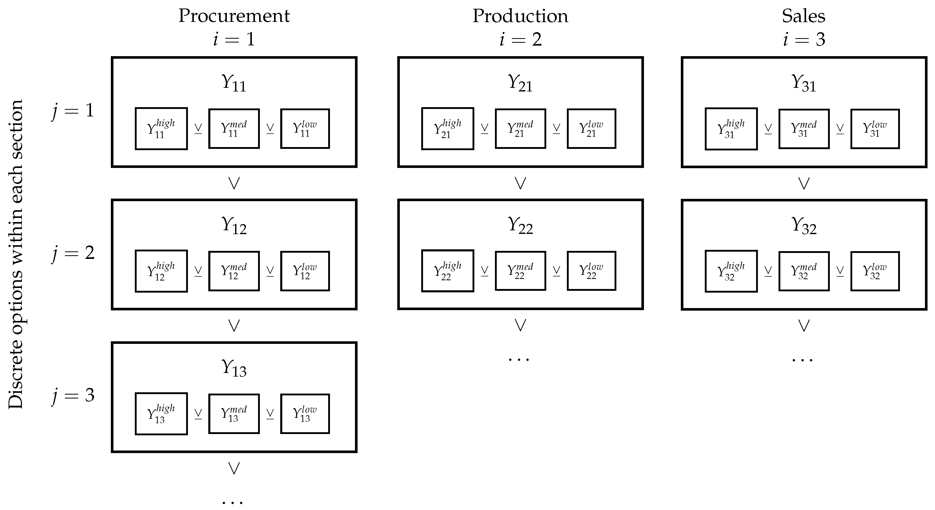
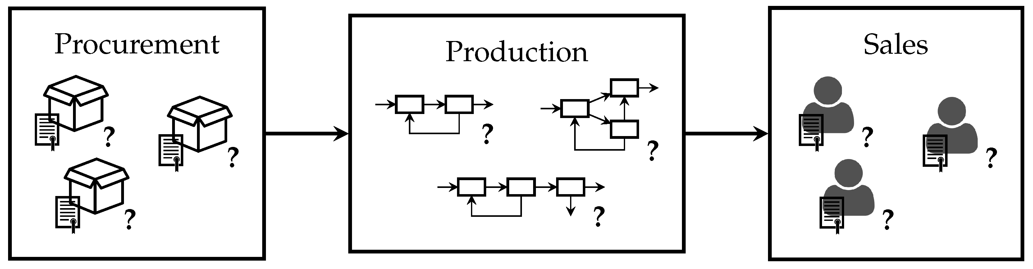
Consider an illustrative chemical production process consisting of three sections: procurement, production, and sales, displayed in Figure 1. We examine this process in more detail in Section 3. Multiple discrete options are available as decision variables for each section, denoted by the Boolean variables $Y_i$, $Y_j$, and $Y_k$ for each section, respectively. For procurement, these discrete decisions may describe selection among several available supply contracts from various vendors. For sales, there might exist several sales opportunities corresponding to different customers. In production, selection among various production modes and capital purchases are often key decisions. For our illustrative process, $Y_{12}=True$ describes the selection of the second procurement contract, for example.

In typical industrial practice, models at varying detail levels are often developed separately from each other, with interoperability suffering as a result. By making use of GDP, the choice of modeling detail can be integrated within a single framework, allowing related models to be developed in proximity to each other. Note that care should still be taken to define appropriate interconnections between the process sections so that relevant phenomena can be described (e.g., time dependence).

In the second case, a modeler may wish to use approximate models in a preliminary analysis to identify promising candidates among numerous alternatives, then drill down into progressively more detailed representations for remaining alternatives. For chemical processes, making assumptions that restrict temperatures, transport phenomena, or thermodynamic complexity can greatly simplify a model representation. However, variations in degrees of freedom and relevant physical phenomena should be subsequently revisited. In specialized simulation software, provisions for changing the thermodynamic assumptions of a chemical process are commonplace. However, the ability to do so is less common in equation-oriented optimization frameworks. Instead, a new model must frequently be developed at the desired complexity level. With GDP, the imposition or relaxation of these assumptions may be made by setting the value of Boolean variables. For a broader perspective, by imposing the implication that selection of unit u requires its modeling at a low detail level, $Y_u\Rightarrow Y_u^{low}$, we can restrict consideration to the approximate models. Conversely, for a deeper perspective, we can consider only more rigorously modeled alternatives by imposing the use of high detail models $Y_u\Rightarrow Y_u^{high}$. Note that at high fidelity, some alternatives may themselves involve selection among a discrete decision space. For example, selection of a distillation column in a chemical process may involve deciding on the number of trays. This discrete decision could itself be treated at various levels of modeling fidelity. Fortunately, with GDP, this decision can simply be nested within the higher-level selection as a nested disjunction [49].

3. Case Study

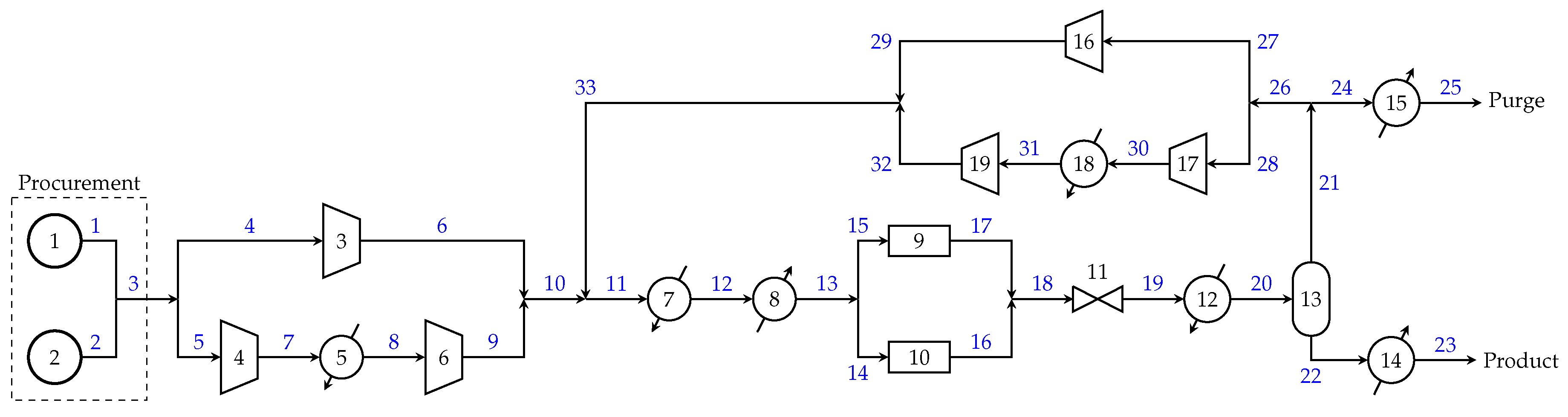
To demonstrate the principles of GDP as a tool for model management, we propose an illustrative end-to-end methanol synthesis process example adapted from literature [22]. As previously stated, the process consists of three sections: procurement, production, and sales (see Figure 2). Procurement must source the syngas from one of two different vendors, each of which offers a different purity-dependent cost schedule per unit feed. Production must select the optimal equipment configuration and operating conditions (temperatures, pressures, flows, and compositions) to convert syngas to methanol. This includes the discrete decision between single and two-stage compression for both the feed and recycle streams, as well as the choice between a higher-conversion, higher-cost reactor and a cheaper variant. Sales then contracts with one of two different customers, who are willing to pay a unit price that depends on the product purity. Each of these sections may be modeled at a high, medium, and low level of detail. The production section superstructure appears in Figure 3, with unit 9 as the cheap reactor alternative with low conversion and unit 10 denoting the expensive reactor with high conversion. Amendments to the literature methanol process synthesis model are presented in Appendix C.

Below, we present a generic formulation for an end-to-end techno-economic analysis model and demonstrate how it may be adapted to our methanol synthesis example. In the following subsections, we lay out the relevant sets, parameters, decision variables, and functions before presenting the formulation. We then discuss manipulations of the formulation for both use cases from Section 2.

3.1. Sets

The chemical process involves a set of components C, which include the relevant raw materials, reaction intermediates, inerts, and products. For the methanol process, we have feed components $H_2$ and $CO$, inert $C{H}_4$, and product $C{H}_{3}OH$. The process is subdivided into three major process sections I: procurement, production, and sales. Of all possible process section alternatives J, a subset $J_i\subseteq J$ is available for selection for each section $i\in I$. In the production section of the methanol process, two of these alternatives are single-stage feed compression, and two-stage feed compression. The process also involves a set of streams K that describe flows of material between process sections. Finally, for each process alternative, a set of modeling detail levels $l\in L$ are available. We consider in our example three detail levels: “low”, “medium”, and “high.”

$c\in C$	Set of components (feeds, intermediates, inerts, and products)
$i\in I$	Set of end-to-end process sections
$j\in J$	Set of process section alternatives
$J_i$	Set of alternatives available for process section i
$k\in K$	Set of streams
$l\in L$	Set of detail levels

3.2. Variables

The decision variables include characterization of each process stream $k\in K$: total molar flowrate $F_k$ and component molar flowrate $f_{kc}$ for each component $c\in C$, as well as the stream temperature $T_k$ and pressure $P_k$. A profit or cost (negative) contribution from each section $i\in I$ is given by $z_i$. This, in turn, may be influenced by the contribution ${\zeta }_{ij}$ from selection of alternative $j\in J_i$ for section $i\in I$. Other continuous state variables x may also be relevant for internal calculations within the alternatives. In the methanol case study, these variables include conversion rates in the reactors and shaft work required in the compressors. Finally, the Boolean variables Y govern selection among the process alternatives and modeling detail levels. $Y_{ij}$ determines whether alternative $j\in J_i$ is active for section $i\in I$. $Y_i^l$ determines whether process section $i\in I$ is modeled at detail level $l\in L_i$. Finally, for each process alternative $j\in J_i$ in section $i\in I$, Boolean $Y_{ij}^l$ determines the modeling detail level $l\in L_{ij}$.

$f_{ck}$	molar flow of component c on stream k
$F_k$	total molar flow of stream k
$T_k$	temperature of stream k
$P_k$	pressure of stream k
$z_i$	profit or cost contribution from section i
${\zeta }_{ij}$	profit or cost contribution from alternative j in section i
x	other continuous state variables
$Y_{ij}$	Boolean selection of process alternative j for section i
$Y_i^l$	Boolean selection of detail level l for modeling process section i
$Y_{ij}^l$	Boolean selection of detail level l for modeling process alternative j in section i

3.3. Functions

The problem-specific variable relationships for the end-to-end process are represented by several functions. The globally relevant constraints $g(f,F,T,P,x)$ describe variable relationships that must be satisfied regardless of discrete selections of the process alternatives or modeling detail levels. These include the linking constraints that equate stream flow properties between different process sections. That is, the exit stream from the procurement section should be equivalent to the inlet stream to the production section. The constraints $r_{ij}(f,F,T,P,x)$ describe the relationships that are enforced regardless of the selected detail level when alternative $j\in J_i$ is selected for section $i\in I$. For each section $i\in I$, the constraints $h_i^l(f,F,T,P,x)$ describe variable interactions at each detail level $l\in L_i$ that are relevant regardless of the selected process alternatives. These constraints include potential equality relationships that link different process alternatives in a section with each other. For each of these alternatives $j\in J_i$, the constraints $s_{ij}^l(f,F,T,P,x)$ describe the variable relationships at detail level $l\in L_{ij}$. Here are included the kinetic calculations for the reactor conversion, or the shaft work calculation for the compressors. The cost functions are computed using ${\varphi }_i^l(f,F,T,P,x,\zeta )$ at the section level, and ${\psi }_{ij}^l(f,F,T,P,x)$ for each process alternative. One common interpretation of ${\varphi }_i^l(f,F,T,P,x,\zeta )$ is given in Equation (3), where the section cost is simply equal to the sum of the contributions ${\zeta }_{ij}$ from each alternative $j\in J_i$, but more complex relationships are possible.

$g(f,F,T,P,x)$	globally relevant constraints
$r_{ij}(f,F,T,P,x)$	constraints relevant to selection of alternative $j\in J_i$ for process section $i\in I$ for any detail level
$h_i^l(f,F,T,P,x)$	constraints describing process section $i\in I$ at detail level $l\in L_i$
$s_{ij}^l(f,F,T,P,x)$	constraints describing alternative $j\in J_i$ for process section $i\in I$ at detail level $l\in L_{ij}$
${\varphi }_i^l(f,F,T,P,x,\zeta )$	calculation of profit or cost contribution for section $i\in I$
${\psi }_{ij}^l(f,F,T,P,x)$	calculation of profit or cost contribution for selecting alternative $j\in J_i$ in section $i\in I$
$\Omega \left(Y\right)$	Logical propositions between Boolean selections

$$z_i={\varphi }_i^l(f,F,T,P,x,\zeta )=\sum _{j\in J_i}{\zeta }_{ij}$$

(3)

3.4. Formulation

The overall generic problem formulation is given in Problem (P1). The objective is to maximize the profit, denoted by Z, equal to the summation of profit (or negative cost) contributions from each section $i\in I$. In the methanol process, we consider revenue from the methanol sales, purchase costs from the syngas feed, utility costs for the heaters and coolers, electricity costs for the compressors, fuel credit for the purge stream, and annualized capital costs for equipment purchases.

$$\begin{array}{cc}\hfill maxZ=& \sum _{i\in I}{z}_i\hfill \end{array}$$

(P1.1)

$$\begin{array}{cc}\hfill s.t.& g(f,F,T,P,x)\le 0\hfill \end{array}$$

(P1.2)

$$\begin{array}{cccc}\hfill & \underset{j\in J_i}{\bigvee }\left[\begin{array}{c}{Y}_{ij}\\ r_{ij}(f,F,T,P,x)\le 0\end{array}\right]\hfill & \hfill & \forall i\in I\hfill \end{array}$$

(P1.3)

$$\begin{array}{cccc}\hfill & \underset{l\in L_i}{\bigvee }\left[\begin{array}{c}{Y}_i^l\\ h_i^l(f,F,T,P,x)\le 0\\ z_i={\varphi }_i^l(f,F,T,P,x,\zeta )\end{array}\right]\hfill & \hfill & \forall i\in I\hfill \end{array}$$

(P1.4)

$$\begin{array}{cccc}\hfill & Y_{ij}\Rightarrow \underset{l\in L_{ij}}{\bigvee }\left[\begin{array}{c}{Y}_{ij}^l\\ s_{ij}^l(f,F,T,P,x)\le 0\\ {\zeta }_{ij}={\psi }_{ij}^l(f,F,T,P,x)\end{array}\right]\hfill & \hfill & \forall i\in I,\forall j\in J_i\hfill \end{array}$$

(P1.5)

$$\begin{array}{cccc}\hfill & \underset{l\in L_i}{\underline{\bigvee }}{Y}_i^l\hfill & \hfill & \forall i\in I\hfill \end{array}$$

(P1.6)

$$\begin{array}{cccc}\hfill & Y_{ij}\Rightarrow \underset{l\in L_{ij}}{\underline{\bigvee }}{Y}_{ij}^l\hfill & \hfill & \forall i\in I,\forall j\in J_i\hfill \end{array}$$

(P1.7)

$$\begin{array}{cccc}\hfill & Y_{ij}^l\Rightarrow Y_{ij}\hfill & \hfill & \forall i\in I,\forall j\in J_i,\forall l\in L_{ij}\hfill \end{array}$$

(P1.8)

$$\begin{array}{cc}\hfill & \Omega \left(Y\right)=True\hfill \end{array}$$

(P1.9)

$$\begin{array}{cccc}\hfill & z_i\in \mathbb{R}\hfill & \hfill & \forall i\in I\hfill \end{array}$$

(P1.10)

$$\begin{array}{cccc}\hfill & z_{ij}\in \mathbb{R}\hfill & \hfill & \forall i\in I,\forall j\in J_i\hfill \end{array}$$

(P1.11)

$$\begin{array}{cc}\hfill & f\in {\mathbb{R}}^{\left|C\right|\left|K\right|}\hfill \end{array}$$

(P1.12)

$$\begin{array}{cc}\hfill & F\in {\mathbb{R}}^{\left|K\right|}\hfill \end{array}$$

(P1.13)

$$\begin{array}{cc}\hfill & T\in {\mathbb{R}}^{\left|K\right|}\hfill \end{array}$$

(P1.14)

$$\begin{array}{cc}\hfill & P\in {\mathbb{R}}^{\left|K\right|}\hfill \end{array}$$

(P1.15)

$$\begin{array}{cc}\hfill & x\in X\subseteq {\mathbb{R}}^{n_X}\hfill \end{array}$$

(P1.16)

$$\begin{array}{cc}\hfill & Y\in {\{True,False\}}^p\hfill \end{array}$$

(P1.17)

(P1.2) describes global constraints that are enforced independent of any alternative or detail selection. Disjunction (P1.3) governs the selection among the process alternatives $j\in J_i$ for each section $i\in I$. Disjunction (P1.4) gives the detail level $l\in L_i$ at which the major process sections $i\in I$ are modeled. Implication (P1.5) states that the selection of an alternative $j\in J_i$ implies the choice of a detail level $l\in L_{ij}$. For each section, the exclusive-OR relationship (P1.6) states that exactly one detail level $l\in L_i$ is used to model alternative-independent interactions. Similarly, for a selection of process alternative $j\in J_i$, Implication (P1.7) governs selection of exactly one detail level $l\in L_{ij}$ for modeling each alternative. Implication (P1.8) enforces that selection of a modeling detail level for an alternative implies that the alternative is selected. Other logical propositions are expressed using $\Omega \left(Y\right)$. Finally, the continuous variable definitions are given in lines (P1.10)–(P1.17).

Note that this illustrative example is meant to give a sense of the complexity that is possible to represent in a process design problem using GDP modeling techniques. GDP modeling easily supports augmentation of the model to consider, for example, methane reforming as another process section. Other process relationships and logical expressions are also possible to include, as the problem demands.

3.5. Discussion

The GDP model in Section 3.4 captures both the choice among discrete process alternatives as well as the level of modeling detail used to describe each alternative. The observant reader may note that the MINLP resulting from the reformulation of this GDP is more complex than simply modeling the entire process in high detail. While true, the power of GDP lies in the ability to systematically activate or deactivate entire blocks of related constraints. The intention of formulation (P1) is not to solve the monolithic GDP model, but rather to systematically generate models that trade off fidelity and tractability for different analyses from a single source of truth by imposing the relevant logical implications. As a result, Problem (P1) could be regarded as a parametric optimization in which the modeler prespecifies the values of $Y_i^l$ to satisfy Equation (P1.6) for each section $i\in I$ and provides logical implications to tie selection of an alternative $Y_{ij}$ to selection of the desired detail level $Y_{ij}^l$ for each alternative $j\in J_i$.

Once these decisions are made, model simplifications driven by logical inference are applied to generate a process model at the desired level of detail for each of its constituent sections. For example, the production team may want to adopt a simplified view of the procurement and sales sections while preserving a high-fidelity view of production section alternatives. To accomplish this, the logical statements in Equation (4) may be appended to the model.

$$\begin{array}{cccc}\hfill Y_i& \Rightarrow Y_i^{low},\hfill & \hfill & i\in \{procurement,sales\}\hfill \\ \hfill Y_i& \Rightarrow Y_i^{high},\hfill & \hfill & i\in \left\{production\right\}\hfill \\ \hfill Y_{ij}& \Rightarrow Y_{ij}^{low},\hfill & \hfill & i\in \{procurement,sales\},\forall j\in J_i\hfill \\ \hfill Y_{ij}& \Rightarrow Y_{ij}^{high},\hfill & \hfill & i\in \left\{production\right\},\forall j\in J_i\hfill \end{array}$$

(4)

Due to the exclusive-OR-type relationship between different levels of modeling detail established by logical statements (P1.6) and (P1.7), this forces the implied level of detail to be selected for its corresponding alternative or section. Applying standard principles of logical inference [21], we arrive at the model shown in Problem (P2), with the sets $I^{low}=\{procurement,sales\}$ and $I^{high}=\left\{production\right\}$.

$$\begin{array}{cc}\hfill maxZ=& \sum _{i\in I}{z}_i\hfill \end{array}$$

(P2.1)

$$\begin{array}{cc}\hfill s.t.& g(f,F,T,P,x)\le 0\hfill \end{array}$$

(P2.2)

$$\begin{array}{cccc}\hfill & \underset{j\in J_i}{\bigvee }\left[\begin{array}{c}{Y}_{ij}\\ r_{ij}(f,F,T,P,x)\le 0\end{array}\right]\hfill & \hfill & \forall i\in I\hfill \end{array}$$

(P2.3)

$$\begin{array}{cccc}\hfill & \left.\begin{array}{c}{Y}_i^{low}=True\\ h_i^{low}(f,F,T,P,x)\le 0\\ z_i={\varphi }_i^{low}(f,F,T,P,x,\zeta )\end{array}\right\}\hfill & \hfill & \forall i\in I^{low}\hfill \end{array}$$

(P2.4)

$$\begin{array}{cccc}\hfill & Y_i^l=False\hfill & \hfill & \forall i\in I^{low},\forall l\in L_i\backslash \left\{low\right\}\hfill \end{array}$$

(P2.5)

$$\begin{array}{cccc}\hfill & \left.\begin{array}{c}{Y}_i^{high}=True\\ h_i^{high}(f,F,T,P,x)\le 0\\ z_i={\varphi }_i^{high}(f,F,T,P,x,\zeta )\end{array}\right\}\hfill & \hfill & \forall i\in I^{high}\hfill \end{array}$$

(P2.6)

$$\begin{array}{cccc}\hfill & Y_i^l=False\hfill & \hfill & \forall i\in I^{high},\forall l\in L_i\backslash \left\{high\right\}\hfill \end{array}$$

(P2.7)

$$\begin{array}{cccc}\hfill & Y_{ij}\Rightarrow \left\{\begin{array}{c}{Y}_{ij}^{low}\\ s_{ij}^{low}(f,F,T,P,x)\le 0\\ {\zeta }_{ij}={\psi }_{ij}^{low}(f,F,T,P,x)\end{array}\right\}\hfill & \hfill & \forall i\in I^{low},\forall j\in J_i\hfill \end{array}$$

(P2.8)

$$\begin{array}{cccc}\hfill & Y_{ij}^l=False\hfill & \hfill & \forall i\in I^{low},\forall j\in J_i,\forall l\in L_i\backslash \left\{low\right\}\hfill \end{array}$$

(P2.9)

$$\begin{array}{cccc}\hfill & Y_{ij}\Rightarrow \left\{\begin{array}{c}{Y}_{ij}^{high}\\ s_{ij}^{high}(f,F,T,P,x)\le 0\\ {\zeta }_{ij}={\psi }_{ij}^{high}(f,F,T,P,x)\end{array}\right\}\hfill & \hfill & \forall i\in I^{high},\forall j\in J_i\hfill \end{array}$$

(P2.10)

$$\begin{array}{cccc}\hfill & Y_{ij}^l=False\hfill & \hfill & \forall i\in I^{high},\forall j\in J_i,\forall l\in L_i\backslash \left\{high\right\}\hfill \end{array}$$

(P2.11)

$$\begin{array}{cccc}\hfill & Y_{ij}^l\Rightarrow Y_{ij}\hfill & \hfill & \forall i\in I,\forall j\in J_i,\forall l\in L_{ij}\hfill \end{array}$$

(P2.12)

$$\begin{array}{cc}\hfill & \Omega \left(Y\right)=True\hfill \end{array}$$

(P2.13)

$$\begin{array}{cccc}\hfill & z_i\in \mathbb{R}\hfill & \hfill & \forall i\in I\hfill \end{array}$$

(P2.14)

$$\begin{array}{cccc}\hfill & z_{ij}\in \mathbb{R}\hfill & \hfill & \forall i\in I,\forall j\in J_i\hfill \end{array}$$

(P2.15)

$$\begin{array}{cc}\hfill & f\in {\mathbb{R}}^{\left|C\right|\left|K\right|}\hfill \end{array}$$

(P2.16)

$$\begin{array}{cc}\hfill & F\in {\mathbb{R}}^{\left|K\right|}\hfill \end{array}$$

(P2.17)

$$\begin{array}{cc}\hfill & T\in {\mathbb{R}}^{\left|K\right|}\hfill \end{array}$$

(P2.18)

$$\begin{array}{cc}\hfill & P\in {\mathbb{R}}^{\left|K\right|}\hfill \end{array}$$

(P2.19)

$$\begin{array}{cc}\hfill & x\in X\subseteq {\mathbb{R}}^{n_X}\hfill \end{array}$$

(P2.20)

$$\begin{array}{cc}\hfill & Y\in {\{True,False\}}^p\hfill \end{array}$$

(P2.21)

Problem (P2) now describes the decision space of the overall process with a focus on the production section. Changing the logical implications in Equation (4), we can easily shift focus in model fidelity to other sections of the process. By imposing different logical relationships on the general GDP model and applying easily automated principles of logical inference, we are able to derive multiple model variants from a single source of truth. Different levels of detail can also be evaluated as a post-solve solution quality check. The modeler can hold constant the production section decisions and increase modeling detail in the other sections to examine impacts of their decision-making on other sections. While this type of analysis may be possible under other engineered frameworks, GDP offers the formalism of an end-to-end perspective that is tied together by mathematical theory.

3.6. Solution Strategies

After generating a variant such as Problem (P2), a solution approach may be selected to obtain the optimal decision values. As previously introduced, the BM and HR reformulations to MINLP are the most popular approaches [2], trading off formulation size versus tightness of the continuous relaxation. The BM formulation for Problem (P2) may be found in Appendix A. For BM, equality constraints in the disjuncts are replaced by their corresponding two inequalities to facilitate relaxation of the constraint. BM results in a smaller problem size, as it does not require the introduction of new variables. However, the use of the Big-M parameter M results in a looser continuous relaxation. Note that the relaxation may be improved by selecting unique values of M for each constraint [48]. For a tighter continuous relaxation, the HR formulation found in Appendix B may be used. HR requires additional disaggregated variables to be defined for each disjunct, so the problem size may be significantly larger than BM. However, the tighter HR formulation may require fewer iterations to converge. Once the reformulation to MINLP is made, the model can be sent to the user’s solver of choice. Direct logic-based decomposition approaches [22,39] are also possible for solving GDP models, with implementations available in Pyomo.GDP via the GDPopt solver [46].

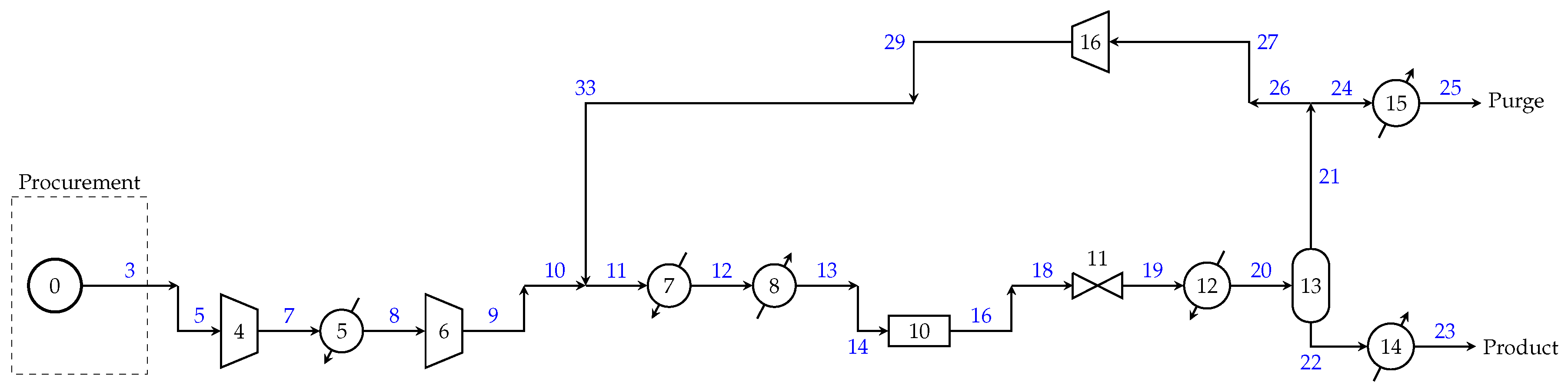
We solve the methanol synthesis model described in Problem (P2) and obtain a solution with annual profit of $1.8 million using two-stage feed compression, the cheap reactor, and single-stage recycle compression, see Figure 4. We can now fix the production section discrete decisions and evaluate the solution at varying detail levels for the procurement and sales sections. The results are given in

Table 1. Profit (1000 USD) at the fixed production section design of two-stage feed compression, the cheap reactor, and single-stage recycle compression compared to the profit achievable when the design is allowed to vary.

Procurement Detail	Sales Detail	Fixed Design	Best Design	Difference
low	low	1793	1793
low	med	1564	1614	single-stage feed compression
low	high	2617	2667	single-stage feed compression
med	low	1793	1793
med	med	1564	1614	single-stage feed compression
med	high	2617	2667	single-stage feed compression
high	low	1709	1832	single-stage feed compression
high	med	1746	1850	single-stage feed compression
high	high	3133	3183	single-stage feed compression

.

Notice that the solution profit tends to increase at higher modeling details for the feed and sales. This is due to the additional flexibility in adjusting coordinating purity levels across procurement, production, and sales. In the high-detail solutions, a higher purity syngas is purchased to enable production of a higher purity methanol product. The supplier and customer contracts are also selected to facilitate the purity decision. The procurement contract is selected with a higher base cost, but lower incremental cost for improved purity. Conversely, the customer contract is chosen where a higher purity is more valued. Thus, despite an increase in feed cost of $4.3 million vs. $3.4 million in the low-detail solution, the product revenue rises to $10.6 million rather than $7.7 million.

The Problem (P2) solution is also compared in Table 1 to the profit possible when the production section configuration is allowed to change at higher procurement and sales modeling detail levels. Here, we see that at higher levels of modeling detail, the single stage feed compressor becomes more advantageous, but only by the $50 thousand margin that accounts for the difference in annualized capital cost. In general, this analysis may not be possible, as the formulation for solving all decision degrees of freedom at a high level of modeling detail may be intractable. However, even at a medium level of sales modeling detail, it is possible to notice that the choice of single-stage feed compression may be relevant in the optimal production configuration.

As an illustration of the flexibility of GDP modeling, another solution approach that can be utilized is to emulate traditional process design strategies. GDP model (P1) is compatible with a design analysis akin to the hierarchical decomposition approach described by Douglas [50], by solving sequentially at different detail levels. First, the overall process (P1) is solved with a low detail level in iteration $iter=0$, enforcing the implications in Equation (5).

$$\begin{array}{ccc}\hfill Y_i^0& \Rightarrow Y_i^{0,low},\hfill & \hfill \forall i\in I\\ \hfill Y_{ij}^0& \Rightarrow Y_{ij}^{0,low},\hfill & \hfill \forall i\in I,\forall j\in J_i\end{array}$$

(5)

The solution to this overview problem gives high-level decisions among the process alternatives and defines the following sets for the iteration $iter=1$. Let $J_i^1=\{j\in J_i:Y_{ij}^0=True\}$ denote the selected alternatives from the overview problem from iteration $iter=0$. In the next iteration, we enforce for (P1) the implications in Equation (6) such that these alternatives are evaluated at a progressively higher detail level.

$$\begin{array}{cccc}\hfill Y_i^1& \Rightarrow Y_i^{1,med},\hfill & \hfill & \forall i\in I\hfill \\ \hfill Y_{ij}^1& \Rightarrow Y_{ij}^{1,med},\hfill & \hfill & \forall i\in I,\forall j\in J_i^1\hfill \\ \hfill Y_{ij}^1& \Rightarrow Y_{ij}^{0,low},\hfill & \hfill & \forall i\in I,\forall j\in J_i\backslash J_i^1\hfill \end{array}$$

(6)

The algorithm would terminate at iteration $iter=N$ when all selected alternatives are evaluated at a high detail level: $Y_{ij}^{high}=True,\forall i\in I,\forall j\in J_i$. Note that solutions at lower detail levels can be used to initialize the higher fidelity models for each alternative, aiding in algorithm robustness. The amount of backtracking done by the algorithm to evaluate other alternatives can be tuned by applying a penalty factor to alternatives modeled at lower detail levels.

We apply this algorithm to the methanol synthesis. In the base iteration ($iter=0$), all alternatives are modeled at a low detail level. The solution gives a configuration of the cheap reactor with two-stage feed compression and single-stage recycle compression at a profit of $1.1 million. The structure for this solution is identical to that shown in Figure 4. We increase the modeling detail level for these selections and solve iteration 1.

Solving the low-detail overview problem, we obtain a configuration using the cheap reactor, two-stage feed compression, and single-stage recycle compression, yielding a profit of $1.1 million. We then increase the level of modeling detail for the selected alternatives. Solving again, we obtain a profit of $0.4 million with the expensive feed alternative, the cheap reactor, two-stage feed compression, single-stage recycle compression, and the high-purity sales option. At this intermediate level of modeling detail, the solution profit decreases because physical constraints are more tightly enforced, but not as many optimization degrees of freedom are made available to the solver yet. For some analyses, it may be advantageous for intermediate detail levels to produce a monotonically tightening approximation of the high-detail representation, but we do not address that consideration in this work. At the next iteration ($iter=2$), we increase the detail level again, obtaining now a profit of $3.1 million, using the contract with supplier 1, the cheap reactor, two-stage feed compression, single-stage recycle compression, and the contract with customer 1. At this point, the algorithm terminates, as all selected alternatives are modeled at the highest possible level of detail.

4. Conclusions

In this paper, we present GDP not only as a mathematical modeling framework supporting advanced solution strategies, but also as a modeling tool to organize model variants. We demonstrate through an illustrative case study that GDP is a useful model abstraction that separates algebraic and logical relationships within a process design problem. From a single GDP model capturing discrete design alternatives as well as alternatives in modeling fidelity, variants can be generated to suit the modeling scope and focus for different process sections by specifying appropriate logical implications. As a result, model interoperability is improved, facilitating simplified post-solution validation analysis. Preservation of model logical structure in GDP also offers the modeler flexibility to reformulate the problem as an MINLP or to apply a variety of automated decomposition methods.

References

- Floudas, C.A.; Gounaris, C.E. A review of recent advances in global optimization. J. Global Optim. 2009, 45, 3–38. [Google Scholar] [CrossRef]
- Trespalacios, F.; Grossmann, I.E. Review of mixed-integer nonlinear and generalized disjunctive programming methods. Chem. Ing. Tech. 2014, 86, 991–1012. [Google Scholar] [CrossRef]
- Lee, J.; Leyffer, S. (Eds.) Mixed Integer Nonlinear Programming; The IMA Volumes in Mathematics and its Applications; Springer: New York, NY, USA, 2012; Volume 154. [Google Scholar] [CrossRef]
- Kronqvist, J.; Bernal, D.E.; Lundell, A.; Grossmann, I.E. A Review and Comparison of sSolvers for Convex MINLP; Springer: New York, NY, USA, 2019; Volume 20, pp. 397–455. [Google Scholar] [CrossRef]
- Dowling, A.W.; Biegler, L.T. A framework for efficient large scale equation-oriented flowsheet optimization. Comput. Chem. Eng. 2015, 72, 3–20. [Google Scholar] [CrossRef]
- Kondili, E.; Pantelides, C.; Sargent, R. A general algorithm for short-term scheduling of batch operations—I. MILP formulation. Comput. Chem. Eng. 1993, 17, 211–227. [Google Scholar] [CrossRef]
- Smith, E.; Pantelides, C. Design of reaction/separation networks using detailed models. Comput. Chem. Eng. 1995, 19, 83–88. [Google Scholar] [CrossRef]
- Bagajewicz, M.J.; Manousiouthakis, V. Mass/heat-exchange network representation of distillation networks. AIChE J. 1992, 38, 1769–1800. [Google Scholar] [CrossRef]
- Friedler, F.; Tarjan, K.; Huang, Y.; Fan, L. Combinatorial algorithms for process synthesis. Comput. Chem. Eng. 1992, 16, S313–S320. [Google Scholar] [CrossRef]
- Farkas, T.; Rev, E.; Lelkes, Z. Process flowsheet superstructures: Structural multiplicity and redundancy Part I: Basic GDP and MINLP representations. Comput. Chem. Eng. 2005, 29, 2180–2197. [Google Scholar] [CrossRef]
- D’Anterroches, L.; Gani, R. Group contribution based process flowsheet synthesis, design and modelling. Fluid Phase Equilibria 2005, 228–229, 141–146. [Google Scholar] [CrossRef]
- Lutze, P.; Babi, D.K.; Woodley, J.M.; Gani, R. Phenomena based methodology for process synthesis incorporating process intensification. Ind. Eng. Chem. Res. 2013, 52, 7127–7144. [Google Scholar] [CrossRef]
- Bertran, M.O.; Frauzem, R.; Sanchez-Arcilla, A.S.; Zhang, L.; Woodley, J.M.; Gani, R. A generic methodology for processing route synthesis and design based on superstructure optimization. Comput. Chem. Eng. 2017, 106, 892–910. [Google Scholar] [CrossRef]
- Wu, W.; Henao, C.A.; Maravelias, C.T. A superstructure representation, generation, and modeling framework for chemical process synthesis. AIChE J. 2016, 62, 3199–3214. [Google Scholar] [CrossRef]
- Li, J.; Demirel, S.E.; Hasan, M.M.F. Process Integration Using Block Superstructure. Ind. Eng. Chem. Res. 2018, 57, 4377–4398. [Google Scholar] [CrossRef]
- Raman, R.; Grossmann, I. Modelling and computational techniques for logic based integer programming. Comput. Chem. Eng. 1994, 18, 563–578. [Google Scholar] [CrossRef]
- Grossmann, I.E.; Trespalacios, F. Systematic modeling of discrete-continuous optimization models through generalized disjunctive programming. AIChE J. 2013, 59, 3276–3295. [Google Scholar] [CrossRef] [Green Version]
- Balas, E. Disjunctive programming and a hierarchy of relaxations for discrete optimization problems. SIAM J. Algebraic Discrete Methods 1985, 6, 466–486. [Google Scholar] [CrossRef]
- Balas, E. Disjunctive Programming; Springer International Publishing: Cham, Switzerland, 2018. [Google Scholar] [CrossRef]
- Raman, R.; Grossmann, I. Relation between MILP modelling and logical inference for chemical process synthesis. Comput. Chem. Eng. 1991, 15, 73–84. [Google Scholar] [CrossRef]
- Hooker, J. Logic-Based Methods for Optimization; John Wiley & Sons, Inc.: Hoboken, NJ, USA, 2000. [Google Scholar] [CrossRef]
- Türkay, M.; Grossmann, I.E. Logic-based MINLP algorithms for the optimal synthesis of process networks. Comput. Chem. Eng. 1996, 20, 959–978. [Google Scholar] [CrossRef]
- Lee, S.; Grossmann, I.E. Global optimization of nonlinear generalized disjunctive programming with bilinear equality constraints: applications to process networks. Comput. Chem. Eng. 2003, 27, 1557–1575. [Google Scholar] [CrossRef]
- Ruiz, J.P.; Grossmann, I.E. Global optimization of non-convex generalized disjunctive programs: A review on reformulations and relaxation techniques. J. Global Optim. 2017, 67, 43–58. [Google Scholar] [CrossRef]
- Williams, H.P. Model Building in Mathematical Programming, 5th ed.; John Wiley & Sons, Ltd.: Hoboken, NJ, USA, 2013. [Google Scholar]
- Chen, Q.; Grossmann, I. Recent developments and challenges in optimization-based process synthesis. Annu. Rev. Chem. Biomol. Eng. 2017, 8, 249–283. [Google Scholar] [CrossRef] [PubMed]
- Rolandi, P.A. The Unreasonable Effectiveness of Equations: Advanced Modeling For Biopharmaceutical Process Development. In Computer Aided Chemical Engineering; Elsevier B.V.: Amsterdam, The Netherlands, 2019; pp. 137–150. [Google Scholar] [CrossRef]
- Siirola, J.D.; Hauan, S. Polymorphic optimization. Comput. Chem. Eng. 2007, 31, 1312–1325. [Google Scholar] [CrossRef]
- Tian, Y.; Demirel, S.E.; Hasan, M.M.; Pistikopoulos, E.N. An overview of process systems engineering approaches for process intensification: State of the art. Chem. Eng. Process. Process Intensif. 2018, 133, 160–210. [Google Scholar] [CrossRef]
- Tsay, C.; Pattison, R.C.; Piana, M.R.; Baldea, M. A survey of optimal process design capabilities and practices in the chemical and petrochemical industries. Comput. Chem. Eng. 2018, 112, 180–189. [Google Scholar] [CrossRef]
- Tula, A.K.; Eden, M.R.; Gani, R. Computer-aided process intensification: Challenges, trends and opportunities. AIChE J. 2019. [Google Scholar] [CrossRef]
- Sitter, S.; Chen, Q.; Grossmann, I.E. An overview of process intensification methods. Curr. Opin. Chem. Eng. 2019. [Google Scholar] [CrossRef]
- Simon, H.A. The architecture of complexity. In Facets of Systems Science; Springer US: Boston, MA, USA, 1991; pp. 457–476. [Google Scholar] [CrossRef]
- Knueven, B.; Laird, C.; Watson, J.P.; Bynum, M.; Castillo, A.; US DOE. Egret v. 0.1 (beta), Version v. 0.1 (beta). 2019. [Google Scholar] [CrossRef]
- Gani, R.; Hytoft, G.; Jaksland, C.; Jensen, A.K. An integrated computer aided system for integrated design of chemical processes. Comput. Chem. Eng. 1997, 21, 1135–1146. [Google Scholar] [CrossRef]
- Kravanja, Z.; Grossmann, I.E. Prosyn—An automated topology and parameter process synthesizer. Comput. Chem. Eng. 1993, 17, S87–S94. [Google Scholar] [CrossRef]
- Miller, D.C.; Siirola, J.D.; Agarwal, D.; Burgard, A.P.; Lee, A.; Eslick, J.C.; Nicholson, B.; Laird, C.; Biegler, L.T.; Bhattacharyya, D.; et al. Next generation multi-scale process systems wngineering framework. Comput. Aided Chem. Eng. 2018, 44, 2209–2214. [Google Scholar] [CrossRef]
- Castro, P.M.; Grossmann, I.E. Generalized disjunctive programming as a systematic modeling framework to derive scheduling formulations. Ind. Eng. Chem. Res. 2012, 51, 5781–5792. [Google Scholar] [CrossRef]
- Lee, S.; Grossmann, I.E. New algorithms for nonlinear Generalized Disjunctive Programming. Comput. Chem. Eng. 2000, 24, 2125–2141. [Google Scholar] [CrossRef]
- Ruiz, J.P.; Grossmann, I.E. A hierarchy of relaxations for nonlinear convex generalized disjunctive programming. Eur. J. Operat. Res. 2012, 218, 38–47. [Google Scholar] [CrossRef] [Green Version]
- Trespalacios, F.; Grossmann, I.E. Cutting plane algorithm for convex generalized disjunctive programs. INFORMS J. Comput. 2016, 28, 209–222. [Google Scholar] [CrossRef]
- Bogataj, M.; Kravanja, Z. Alternative mixed-integer reformulation of Generalized Disjunctive Programs. Comput. Aided Chem. Eng. 2018, 43, 549–554. [Google Scholar] [CrossRef]
- Furman, K.C.; Sawaya, N.; Grossmann, I. A computationally useful algebraic representation of nonlinear disjunctive convex sets using the perspective function. Optim. Online 2017. [Google Scholar]
- Brook, A.; Kendrick, D.; Meeraus, A. GAMS, a user’s guide. ACM SIGNUM Newslett. 1988, 23, 10–11. [Google Scholar] [CrossRef]
- Vecchietti, A.; Grossmann, I.E. LOGMIP: A disjunctive 0-1 non-linear optimizer for process system models. Comput. Chem. Eng. 1999, 23, 555–565. [Google Scholar] [CrossRef]
- Chen, Q.; Johnson, E.S.; Siirola, J.D.; Grossmann, I.E. Pyomo.GDP: Disjunctive Models in Python. In Proceedings of the 13th International Symposium on Process Systems Engineering; Eden, M.R., Ierapetritou, M.G., Towler, G.P., Eds.; Elsevier B.V.: San Diego, CA, USA, 2018; pp. 889–894. [Google Scholar] [CrossRef]
- Hart, W.E.; Laird, C.D.; Watson, J.P.; Woodruff, D.L.; Hackebeil, G.A.; Nicholson, B.L.; Siirola, J.D. Pyomo—Optimization Modeling in Python, 2nd ed.; Springer Optimization and Its Applications; Springer International Publishing: Cham, Switzerland, 2017; Volume 67. [Google Scholar] [CrossRef]
- Trespalacios, F.; Grossmann, I.E. Improved big-M reformulation for generalized disjunctive programs. Comput. Chem. Eng. 2015, 76, 98–103. [Google Scholar] [CrossRef]
- Vecchietti, A.; Grossmann, I.E. Modeling issues and implementation of language for Disjunctive Programming. Comput. Chem. Eng. 2000, 24, 2143–2155. [Google Scholar] [CrossRef]
- Douglas, J.M. A hierarchical decision procedure for process synthesis. AIChE J. 1985, 31, 353–362. [Google Scholar] [CrossRef]
- Grossmann, I.E.; Lee, S. Generalized convex disjunctive programming: Nonlinear convex hull relaxation. Comput. Optim. Appl. 2003, 26, 83–100. [Google Scholar] [CrossRef]
Figure 1.
Example process illustrating the embedding of multiple detail levels within discrete options for each process section.
Figure 2.
Simplified process diagram for the illustrative example. Three sections exist: procurement, production, and sales. In each section, decisions must be made in both discrete and continuous variable domains.
Figure 3.
Methanol process flowsheet superstructure, adapted from [22], showing stream numbers in blue.
Figure 4.
Solution flowsheet for Problem (P2), using two-stage feed compression, the cheap reactor, and single-stage recycle compression. At low procurement modeling detail, no feed selection decisions are made.