
A Novel Parallel Simulated Annealing Methodology to Solve the No-Wait Flow Shop Scheduling Problem with Earliness and Tardiness Objectives


1
AN-EL Anahtar ve Elektrikli Ev Aletleri Sanayi A.S., Istanbul 34896, Turkey
2
Industrial Engineering Doctorate Programme, Institute of Pure and Applied Sciences, Marmara University, Istanbul 34722, Turkey
3
Department of Industrial Engineering, Marmara University, Istanbul 34854, Turkey
*
Author to whom correspondence should be addressed.
Processes 2023, 11(2), 454; https://doi.org/10.3390/pr11020454
Submission received: 20 December 2022
/
Revised: 20 January 2023
/
Accepted: 28 January 2023
/
Published: 2 February 2023
(This article belongs to the Special Issue Production Scheduling and Optimization Control on Advanced Manufacturing)
Abstract
:In this paper, the no-wait flow shop problem with earliness and tardiness objectives is considered. The problem is proven to be NP-hard. Recent no-wait flow shop problem studies focused on familiar objectives, such as makespan, total flow time, and total completion time. However, the problem has limited studies with solution approaches covering the concomitant use of earliness and tardiness objectives. A novel methodology for the parallel simulated annealing algorithm is proposed to solve this problem in order to overcome the runtime drawback of classical simulated annealing and enhance its robustness. The well-known flow shop problem datasets in the literature are utilized for benchmarking the proposed algorithm, along with the classical simulated annealing, variants of tabu search, and particle swarm optimization algorithms. Statistical analyses were performed to compare the runtime and robustness of the algorithms. The results revealed the enhancement of the classical simulated annealing algorithm in terms of time consumption and solution robustness via parallelization. It is also concluded that the proposed algorithm could outperform the benchmark metaheuristics even when run in parallel. The proposed algorithm has a generic structure that can be easily adapted to many combinatorial optimization problems.
1. Introduction
Flow shop scheduling problems (FSSPs) consist of jobs that should be processed on different machines. In the classical FSSP, it is assumed that there exists an unlimited buffer between two successive machines. The no-wait flow shop scheduling problem (NWFSSP) is a special case of the generic FSSP in that each operation of a job has to be processed immediately after the preceding operation, without any delay. Consequently, the problem has a permutation schedule that should be processed on no-buffer machines [1]. The permutation constraint ensures that all jobs are processed in the same order on the machines [2]. The NWFSSP is fundamental to applications in real-life production environments, especially for jobs including quick obsolescence risk for manufactured products or their components. Examples are processes of canned food, critical operations of metals while forging, and production with chemical reactions [3].
Graham et al. [4] introduced the notation to define a scheduling problem, where stands for the machine environment, denotes any special constraint, and represents the objective function or functions of the problem. The machine environment shows the shopfloor setup, such as parallel machines, flow shop, and job shop. The constraints present the special cases of processes such as permutation (prmu), no-wait (nwt), blocking (block), and recirculation (rcrc). The last field hosts the objectives, e.g., total completion time, makespan, flow time, earliness, and tardiness. In this study, the NWFSSP is considered to minimize total earliness and tardiness that is denoted by . NWFSSP problems with machines have been proven to be NP-hard in the strong sense, where is higher than 3 [5]. There are a considerable number of published studies that dealt with the NWFSSP with makespan, total completion time, or only tardiness objectives. Correspondingly, total earliness and tardiness objectives may be encountered in many studies dealing with scheduling problems. In some studies, the due date was also included in the model as a constraint rather than an objective. The survey by Allahverdi [6] covered over 300 papers in the literature containing no-wait constraints. The problem with the notation that considers minimizing only total tardiness was recently studied by Aldowaisan and Allahverdi [7], Liu et al. [8], and Ding et al. [9]. However, a relatively small body of literature is concerned with the NWFSSP by minimizing total earliness and tardiness. Some studies [10,11,12,13,14,15,16] built the problem to minimize multiple objectives by integrating due date constraints and objectives such as makespan, total flow time, and resource consumption. Huang et al. [17] studied the flexible FSSP to minimize total weighted earliness and tardiness under the due-window constraint. Some of these studies had the goal of minimizing total tardiness and earliness with minor nuances. Arabameri and Salmasi [18] handled the weighted objective under a sequence-dependent setup time constraint providing a mixed-integer linear programming (MILP) model and a timing algorithm, comparing the performance of the customized particle swarm optimization (PSO) and tabu search (TS) metaheuristics. Schaller and Valente [19] studied the NWFSSP by minimizing total earliness and tardiness and compared dispatching heuristics. They compared the dispatching heuristics under the additional time-allowed constraint in another study [20]. Guevara-Guevara et al. [21] proposed a GA algorithm for the problem under a sequence-dependent setup time constraint and compared it with dispatching heuristics. Zhu et al. [22] implemented a discrete learning fruit fly algorithm for the distributed NWFSSP with weighted objectives under the common due date constraint and compared it to only iterated greedy with idle time insertion evaluation. Qian et al. [23] applied the matrix cube-based estimation of distribution algorithm (MCEDA) under sequence-dependent setup time and release time constraints, benchmarked with seven metaheuristic algorithms.
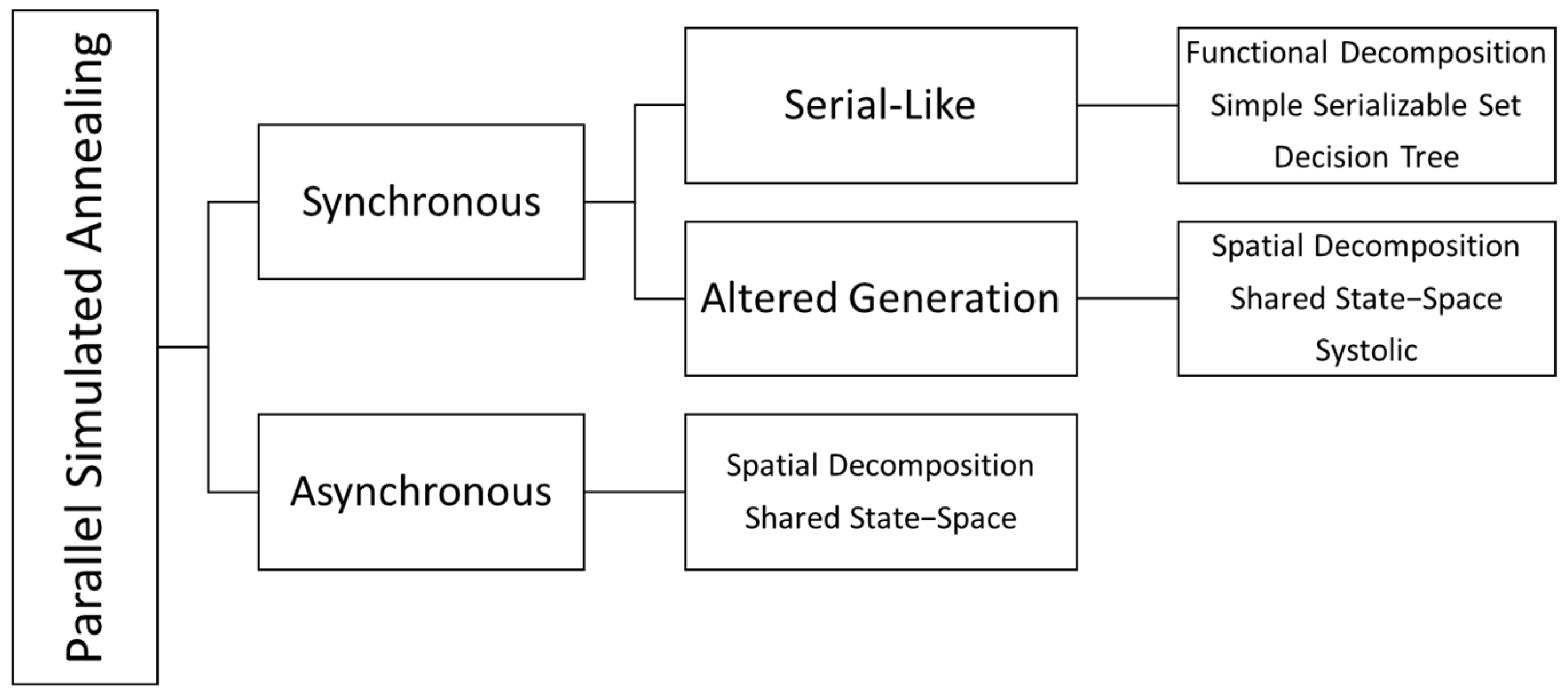
Ingber [24] addressed the primary shortcoming of the SA algorithm as its time-consuming computational steps. Due to its oscillation during the search for alternative solutions, the algorithm requires extensive time to present reasonable incumbent solutions. Many parallelized versions have been developed to overcome this disadvantage. Figure 1 includes the taxonomy by Greening [25] that was produced during his doctoral dissertation.
Greening [25] divided parallel simulated annealing (PSA) algorithms into two main categories. Synchronous algorithms share information during runtime, while asynchronous algorithms have limited or no communication. Synchronous algorithms calculate the same cost function. Asynchronous algorithms work faster by ignoring synchronization and allowing errors but result in lower outcome quality. Synchronous algorithms are divided into two subcategories: serial-like and altered generation. Serial-like algorithms generate new states as applied in a sequentially running algorithm. Altered generation applies different strategies for state generation.
In the past years, many studies have been proposed to overcome the disadvantages of the SA algorithm. Fast simulated annealing (FSA) by Szu and Hartley [26] and very fast simulated reannealing (VFSA) by Ingber [27] are among the prominent studies that altered the cooling process for more rapid convergence to the global minimum. Malek et al. [28] proposed a parallel SA strategy to solve the TSP problem in which parallel algorithms compare their solutions at a certain timepoint and restart with the initial temperature with the incumbent solution. On the basis of these studies, Yao [29] proposed a new simulated annealing algorithm (NSA) that is exponentially faster compared to VFSA. With a different approach, Roussel-Ragot and Dreyfus [30] suggested a general parallel form with two different temperature regimes. In this approach, parallel processors are in touch to update the approved current solution globally when a move is accepted. Mahfoud and Goldberg [31] integrated SA into the genetic algorithm to enrich the population at each iteration. Lee and Lee [32] evaluated various types of moving schemes for parallel synchronous and asynchronous SA strategies with multiple Markov chains. Wodecki and Bożzejko [33] implemented a parallel SA version considering the flow shop problem with a makespan objective in which parallel threads run simultaneous searches. In this implementation, incumbent solutions of all threads are changed to new ones if a thread finds a better solution than the current best solution. As a similar approach to this study, Bożejko and Wodecki [34] developed a procedure that runs a master thread and multiple slave threads. The slave threads iteratively search for better solutions. Upon finding a better incumbent solution, a thread tries intensification iterations and reports the result. All slave threads run again on the new incumbent solution with different temperatures. The results of the study demonstrated average values away from the optimum solution even for 20 jobs. The possible root cause of this failure could be premature convergence due to the greedy intensification of threads inconsistent with the cooling process of the SA algorithm. Czapiński [35] worked on the permutation flow shop problem in order to reduce total flow time. The study included master and worker nodes. Worker nodes obtain feedback on their results after a certain number of iterations to the master node. The incumbent solution is updated by the best solution shared with the master node. Worker nodes run again with the updated incumbent solution as the initial solution. Ferreiro et al. [36] implemented parallel-running asynchronous graphics processing unit (GPU) threads beginning with the same instructions but different initial solutions. Sonuc et al. [37] coded another GPU algorithm on the Compute Unified Device Architecture (CUDA) platform that runs independent threads to solve the binary knapsack problem. Richie and Ababei [38] provided a synchronous methodology with a managing thread that distributes the calculations to the worker threads. Turan et al. [39] suggested the multithread simulated annealing (MTSA) algorithm with master and slave threads. The created slave thread continues running until the defined number of non-improving iterations. Non-improving indicates that the global best solution cannot be improved. Upon completion of the thread runs, solutions are gathered into the pool. Vousden [40] compared the performances of asynchronous and synchronous SA implementations with regard to race conditions. Zhou et al. [41] benchmarked multiple threads of SA without communication initialized with different solutions. Coll et al. [42] built synchronous GPU threads that communicate in predefined time intervals and resume their runs on the best incumbent solution so far. Yildirim [43] deployed a multithread methodology with a hybrid structure where SA is fed by optimizer sub-threads. Even though many further studies are present in the literature, this review covered most of the parallelization approaches.
In the remainder of this paper, an MILP model is introduced to define the research problem. A simulated annealing (SA) metaheuristic variant, namely, the simulated annealing multithread (SAMT) algorithm, is proposed to solve the problem. The contributions of this algorithm and study are as follows:
- Improving the runtime drawback of the SA algorithm;
- Enhancing its robustness to converge to the global optimum solution;
- Providing a new solution approach to NWFSSP, minimizing total earliness and tardiness;
- Enabling parallel processing without excessive resource allocation.
The motivation behind this study is an aim to contribute to improvements in field optimization, more specifically metaheuristics. Even though metaheuristics were introduced after intense studies and analysis, there are still open issues to be optimized. A good example is the study by Deng et al. [44], where the authors improved the mutation strategy of the differential evolution algorithm and even compared the novel methodology to the previously improved differential evolution algorithm methodologies. Similarly, Cai et al. [45] worked on the quantum-inspired evolutionary algorithm to improve multiple shortcomings, such as poor runtime, search capability, and difficulty in assigning rotation angles. With the same focus, this study introduces a novel methodology that improves the original SA without requiring excessive computational resources. Section 2 of the paper states the research problem and details the proposed and benchmark metaheuristic algorithms. Section 3 introduces the benchmark results and comparative analysis. Section 4 includes the discussion, conclusion, and future prospects.
2. Methodology
The NWFSSP imposes processing of the jobs without interruption from the beginning on the first machine until completion on the last machine. Since the objective function also includes minimization of earliness in addition to tardiness, adding a delay between jobs may improve the objective function value (OFV) by avoiding the early completion of a job. However, unforced idleness would not be practical in most cases of the NWFSSP [46]. The disadvantages may be operational costs, such as machine running costs, setup costs, and buffer costs that exceed any cost incurred due to earliness. As a result, the problem is proposed to have a non-delay schedule. An MILP model is suggested to formulate the problem. To provide integrality, two dummy jobs with zero processing times on all machines should be added to the model as the initial and last jobs. Thus, the MILP model has jobs and machines. Each job may be processed only on one machine at a time. Similarly, one machine can process only one job at a time. The proposed MILP model, its parameters, and its decision variables are outlined below.
- Parameters:
- = Slack time between completion time of and starting time of on , if is processed immediately after .
- = a very large number.
- Decision variables:
- = Earliness of .
- = Tardiness of .
- = Completion time of on .
- = 1, if is processed immediately after , and 0 otherwise.
The MILP model on NWFSSP minimizing total earliness and tardiness:
where the objective function in Equation (1) minimizes the sum of total earliness and tardiness; the constraint in Equation (2) ensures that the completion time of a job on a machine is the summation of the completion time of the preceding job, the slack time between these jobs, and the processing time of the job; the constraint in Equation (3) guarantees that the completion time of the first job is its total processing time on all machines; the constraint in Equation (4) calculates the earliness or tardiness by comparing the completion time and due date of each job; and the constraints in Equations (5) and (6) ensure that each job has only one predecessor and successor, respectively. The model consists of jobs to satisfy the constraints in Equations (5) and (6). Equation (7) is a virtual constraint that assigns the first (dummy) job as the predecessor of the last (dummy) job. It is assumed that each job is processed without any delay once any operation of the predecessor job does not cause any violation for no-wait processing to be aligned with real-world applications. Thus, the values of slack time are fixed for any consecutive jobs independent from their position in the schedule. The calculation of is broadly explained by Röck [47].
2.1. Neighborhood Operations
Neighborhood operations are applied to reveal neighbor solutions for metaheuristic algorithms. The types of neighborhood operations influence the performance of a metaheuristic algorithm. Thus, selecting the appropriate operations is the crucial key to exploring the search space wisely. Three different types are considered in this paper that are implemented in the proposed or benchmark algorithms.
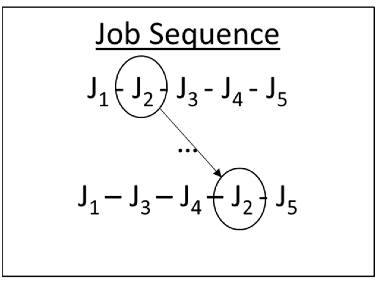
2.1.1. Insert Operation
The insert operation embraces the insertion of a job in the sequence to a specified position. Two positions should be determined for this operation. Usually, these positions are generated randomly or tried successively in an order. Let and be integer numbers from the set . In an insert operation, is removed from the sequence and inserted into the position prior to . The positions of the jobs after slide toward the end of the schedule. An example operation is shown in Figure 2, where Job 2 is inserted into Position 4.
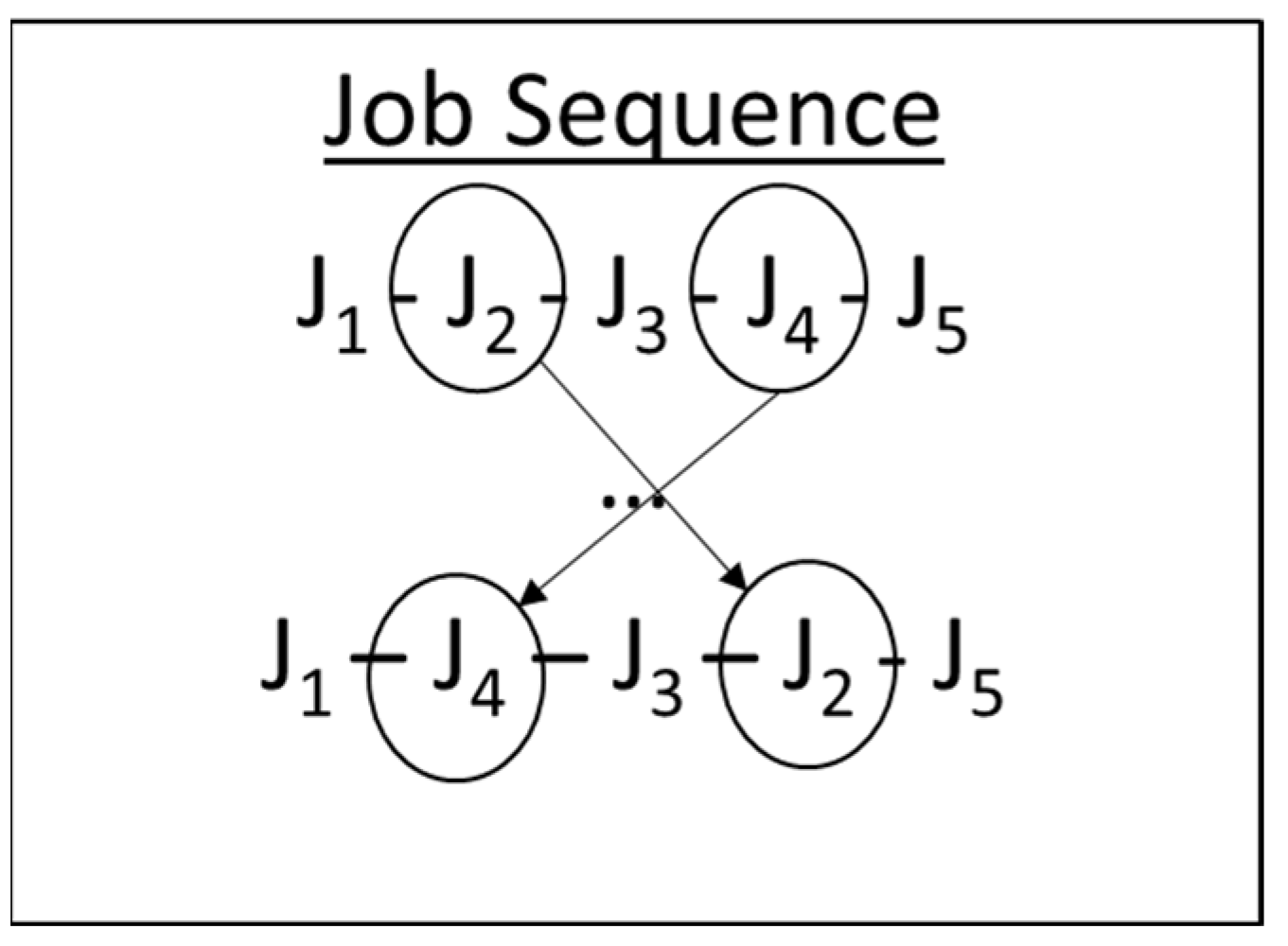
2.1.2. Swap Operation
Congruently to an insert operation, two positions should be determined for swap operations. Let and be integers from the set . In the swap operation, the positions of and are changed mutually. The positions of the remaining jobs do not change. The example in Figure 3 shows the swap operation of Job 2 and Job 4.
2.1.3. Sub-Interchange Operation
Defined by Arabameri and Salmasi [18], sub-interchange is executed by changing two adjacent jobs and . It is believed that running sub-interchange operations after updating the incumbent solution may result in a better solution.
2.2. Proposed Algorithm—Simulated Annealing Multithread (SAMT)
The SAMT algorithm is based on the simulated annealing (SA) metaheuristic. Proposed by Kirkpatrick [48], the SA simulates the annealing process of solids to solve combinatorial optimization problems. In physics, annealing specifies the process in which solids are heated rapidly to a maximum temperature and cooled down slowly in heat baths to allow them to arrange themselves in the ground state of the solid [49]. The algorithm is initialized with a high temperature and cooled slowly. These moves during the cooling process avoid algorithm trapping in local optima [50]. The flow of the classical SA algorithm is stated in Algorithm 1 [51].
| Algorithm 1 Simulated Annealing |
| 1: Select an initial solution in the solution space |
| 2: Set the initial temperature , |
| 3: Set the temperature iteration counter , |
| 4: Set the maximum number of repetitions |
| 5: While (Stopping criteria are not met) |
| 6: Set , |
| 7: While () |
| 8: Generate a new solution |
| 9: Calculate |
| 10: If () |
| 11: Set |
| 12: Else |
| 13: If () |
| 14: Set |
| 15: Set |
| 16: Do |
| 17: Set |
| 18: Set |
| 19: Do |
A review of the literature suggests that there are still open fields for parallel implementation of the SA algorithm. In this study, a novel approach including the utilization of multiple threads is proposed. The simulated annealing multithread (SAMT) algorithm is proposed to overcome the time disadvantage of the classical SA algorithm and boost the convergence process. The algorithm is named after its pragmatic structure in which classical SA runs on a main thread supported by a sub-thread that iteratively updates the incumbent solution of the main thread with much faster SA runs. Rather than distributing the calculations of the algorithm to available processors, this parallelism aims to run different SAs simultaneously to improve the consumed time and search the solution space intelligently to find the global optimum. The SAMT algorithm falls into the altered generation class of synchronous algorithms considering Greening’s taxonomy [25] with shared memory. The novel methodology flow is demonstrated in Algorithm 2.
| Algorithm 2 Simulated Annealing Multithread (SAMT) |
| 1: Select initial solutions in the solution space |
| 2: Set the initial temperature |
| 3: Set the temperature iteration counter |
| 4: Set the maximum number of repetitions |
| 5: Set the operator selection probability |
| 6: Set the fast sub-thread’s initial temperature |
| 7: Set the slow sub-thread’s initial temperature |
| 8: Set the fast sub-thread iteration counter |
| 9: Set the fast sub-thread iteration counter |
| 10: Set the thread selection probability coefficient |
| 11: MAIN THREAD: |
| 12: While (Stopping criteria are not met) |
| 13: If (SUB-THREAD is not running) |
| 14: Calculate |
| 15: If () |
| 16: Set |
| 17: Else |
| 18: Set |
| 19: Run (SUB-THREAD) |
| 20: Set , |
| 21: While |
| 22: If ( |
| 23: |
| 24: Else |
| 25: |
| 26: Calculate |
| 27: If () |
| 28: Set |
| 29: Else |
| 30: If () |
| 31: Set |
| 32: Set |
| 33: Do |
| 34: Set |
| 35: Set |
| 36: Do |
| 37: Return and |
| 38: SUB-THREAD: |
| 39: If () |
| 40: While (Stopping criteria are not met) |
| 41: Set , |
| 42: While |
| 43: If |
| 44: |
| 45: Else |
| 46: |
| 47: Calculate |
| 48: If () |
| 49: Set |
| 50: Else |
| 51: If () |
| 52: Set |
| 53: Set |
| 54: Do |
| 55: Set |
| 56: Set |
| 57: Do |
| 58: Else |
| 59: While (Stopping criteria are not met) |
| 60: Set , |
| 61: While |
| 62: If |
| 63: |
| 64: Else |
| 65: |
| 66: Calculate |
| 67: If () |
| 68: Set |
| 69: Else |
| 70: If () |
| 71: Set |
| 72: Set |
| 73: Do |
| 74: Set |
| 75: Set |
| 76: Do |
The methodology should be initialized by the setting of parameters. Prior to finalizing this methodology, several alternative policies are considered, compared, and tested in terms of simplicity, runtime, efficiency, and implementation complexity. These policies include a different number of threads with distinct completion times and different schemes of solution updates. The threads in the proposed methodology have different roles. The fast thread decreases the runtime by jumping to better solutions in the vicinity of the current best solution with faster steps. This thread may also manipulate the search by orienting the direction toward different “hills” if the thread provides a better solution. The slow thread has different aims, such as enabling moves to longer distances in the vicinity, jumping to similar solutions of nearby optima, or diverging from local optima. Possible jumps after the completion of a sub-thread are presented in Figure 4.
If the sub-thread results in a solution sequence with a better OFV than the global incumbent solution, the global incumbent solution is updated. An adaptive strategy with a single sub-thread provided the best solutions After some experimental runs with different parameters, the results also showed that adjusting the initial temperature and runtime of the sub-thread should be adaptive to achieve elite results. Therefore, the methodology is revised to have a single master (main) thread and a slave (sub) thread, and the assignment of the algorithm speed (slow or fast) is conducted dependent on a predefined parameter. This strategy attempts to seek a larger space and decreases the probability to be stuck in local optima due to premature convergence. Both insert and swap operators work well on the NWFSSP. Both operators are utilized in the proposed methodology to benefit from each and avoid becoming trapped in a cycle. At each iteration, the algorithm runs the insert operator with the probability or the swap operator with the probability . The temperature-dependent type selection function in the first line of the sub-thread determines the type of sub-thread depending on the temperature of the main thread. The value of the constant determines the initial probabilities to select a fast or slow thread. In cases where , the slow thread has a lower probability to be selected at the beginning of the run and the probability increases while decreases. If , then the fast thread has the advantage with a higher probability. The value grants equal probability during all the runs.
2.3. Benchmark Algorithms
The variants of tabu search (TS) and particle swarm optimization (PSO) in the study by Arabameri and Salmasi [18] were selected as benchmark algorithms since these metaheuristics were applied to the same research problem. The benchmark algorithms are introduced in Appendix A, where item A1 introduces the TS and its variants: TS with the EDD initial solution and insertion neighborhood (TSEI), the TS algorithm with a random initial solution and insertion neighborhood (TSRI), the TS algorithm with the EDD initial solution and swap neighborhood (TSES), and the TS algorithm with a random initial solution and swap neighborhood (TSRS); while item A2 describes the PSO algorithm supported by integrating two different local search algorithms: insertion (PSOI) and variable neighborhood structure (PSOV).
2.4. Test Problems
The test problems are selected from the datasets already introduced by different studies. These problems are widely considered in the literature for benchmark purposes of scheduling problems. The proposed and benchmark algorithms are verified on Carlier’s dataset [52], which has eight small-sized problems with 7–14 jobs and 4–9 machines. The process times in the dataset are generated with a pattern of sorting the digits adjacently. Another dataset for benchmarking consists of the scheduling problems defined by Reeves [53]. Reeves generated this dataset to test his proposed genetic algorithm to solve the FSSP problem. The reason for generating this dataset was his failure to find a publicly shared dataset for this purpose since there is some evidence that process times cannot be completely random [54]. Reeves generated this dataset using the suggestions by Rinnooy [55] and his parameters. The dataset has a maximum of 75 jobs and 20 machines beginning from 20 jobs and five machines. The famous Taillard dataset [56] is also included for comparison of the algorithms. The dataset comprises problems with a range of 20–500 jobs and 5–20 machines. Taillard included in his dataset hard problems to be solved. The process times are created randomly from a uniform distribution . Due to the high number of problems, only the first problems with the same number of jobs and machines in the datasets by Reeves and Taillard are considered.
Due dates for the problems are created according to the rule proposed by Arabameri and Salmasi [18]. The due date may be randomly produced from the interval in Equation (10).
where is the lower bound of the makespan, is the tightness factor, and is the range parameter. The and values are selected from the set . To avoid the possibility of negative due date creation, and combinations are ignored for and , respectively. Hence, a total of 27 different problems are solved with seven different due date schemes, resulting in 189 combinations. Among the methods to calculate the in the literature, the method by Taillard [56] is preferred due to its concrete and meaningful structure. The can be calculated according to Equation (11).
where , , and are formulated according to Equations (12)–(14), respectively.
The problems are divided into three groups according to their sizes considering the number of jobs. Small-sized problems in Group 1 have up to 20 jobs to be processed. Medium-sized problems in Group 2 consist of 20–100 jobs. Large-sized problems in Group 3 consist of over 100 jobs.
3. Results
3.1. Results of the Benchmark Runs
All of the metaheuristics involved in this study have several parameters that should be tuned to achieve favorable solutions. Additionally, the common parameters for benchmark runs should be determined. The maximum runtime of any run is limited by a function considering the number of jobs, as stated in Table 1. All metaheuristics except the TSEI and TSES algorithms are initialized with a random sequence to avoid any bias. The TSEI and TSES algorithms are initialized with the sequence provided by the EDD rule in which the jobs with earlier due dates are processed earlier.
The initial temperature of the SA algorithm should be set to a value that allows acceptance of worse solutions with a determined probability, decreasing systematically. Since the test runs are terminated according to the runtime criteria for all algorithms, the temperature of the SA algorithm is intended to be decreased as a function of time according to Equation (15) in this study.
The parameter in Equation (15) denotes the elapsed time, whereas is the total assigned runtime. The algorithm stops when the temperature drops to zero. Similarly, the temperatures of the main and support threads of the SAMT algorithm should also be managed for smooth synchronization. However, the time limit of the threads should be arranged within the time limits of the main thread. Tuning the parameters has a high influence on the performance of a metaheuristic. The guideline by LaTorre et al. [57] identifies several methods that have gained recent attention to tune the parameters of metaheuristic algorithms. The focus iterative local search (FocusILS) methodology [58] was preferred to tune the parameters of the SAMT algorithm. was selected from a set increasing by 50 until 500 degrees. The set {0.25, 0.50, 0.75} was assigned to find the best value of constant and . and were tuned by dividing up to 10. The initial temperature of the SAMT algorithm may be selected as half of the SA algorithm for better and faster convergence. Insert or swap operators are selected with equal probability at each iteration. Running the fast thread more frequently at the initial phase of the algorithm eases discovering the vicinity of the current solution. Rare searches with a slower thread at this phase produce faster jumps toward the optima region if possible. The probability of using the slow thread toward the end of the runtime should be increased. This change is needed to allow the sub-thread to jump from local optima to different optimum regions by climbing the hills. Setting the parameter to 0.25 assigns the probability of running the fast thread to 0.75 and the slow thread to 0.25. The probability of the fast thread decreases and the slow thread increases linearly during runtime until the probability of selecting the fast thread stabilizes at 0.25 and that of the slow thread stabilizes at 0.75. The parameters of the SAMT algorithm are shown in Table 2.
The PSO algorithm is dependent on various parameters and variables that directly affect the performance of the algorithm. Tuning these parameters with ineligible strategies may lead to disadvantages, such as premature convergence or failing to converge to the region near the optimum solution. The constants and variables are set to the values suggested by Arabameri and Salmasi [18] to achieve a consequential benchmark environment. The settings for the PSO algorithm are shown in Table 3.
While the value for the PSOV algorithm is set to a fixed value, the value for the PSOI algorithm is updated regularly at each iteration dependent on a maximum number of iterations and current iteration .
The metaheuristics are compared with the percentage gap (PG), which is the relative percentage deviation of the algorithm compared to the best solution. PG may be calculated according to Equation (16).
where is the OFV value of the selected algorithm, and is the minimum OFV value provided by all algorithms for the corresponding problem. Since the metaheuristics have a stochastic nature, all metaheuristics had triple runs for each benchmark problem. The result tables show the average PG of three runs at each problem. SAMT has a main thread and a sub-thread during its runs. For the sake of fairness, the benchmark algorithms were run twice at each iteration, and the better solution was selected as if they ran two threads asynchronously. Algorithms were coded in the C# programming language. The codes were compiled and run on a single computer with Intel(R) Core (TM) i7-6500U CPU and 8 GB RAM.
The accuracies of the metaheuristic algorithms were verified by comparing them with the MILP results solved on the Carlier dataset. Each problem in the dataset was assigned seven due dates with different due dates creating schemes resulting in 56 test problems. The problems were solved using the Gurobi Solver optimally. Each algorithm could find the optimal result for each problem.
The results of the Reeves dataset are shared in Table A1 of Appendix B. The table has solutions for 49 problems. The last digit in the problem names represents the index for the due date scheme. The results of the Taillard dataset are shown in Table A2 of Appendix B. The table contains 84 problems. The indices and corresponding TF and R values for due date creation are shown in Table 4.
3.2. Comparative Analyses
The algorithms are evaluated under identical conditions and on the same test problems. Therefore, comparative analyses are performed through analysis of variance (ANOVA) considering solutions of the benchmark in terms of the robustness of the results. The two-way ANOVA results in Table 5 reveal that the factors job and algorithm, as well as their interaction, have a significant effect on the values of PG.
Due to the significance, post hoc analyses were conducted to reveal the differences in the group × algorithm interaction with pairwise comparisons. A concern during this analysis is keeping the family-wise error rate under control [57]. Tukey’s HSD (honestly significant difference) and Scheffe tests were applied for pairwise comparisons. Tukey’s HSD has a high sensitivity for pairwise comparisons in balanced conditions while the Scheffe method maintains the family-wise error rate under strict control [59]. A p-value lower than 0.05 shows that the instances are significantly different. Small-sized problems, in terms of the number of jobs, are not taken into consideration for evaluation since all the algorithms return the same OFV for all problems in this group.
The comparison results of Tukey’s HSD statistics for medium-sized problems are demonstrated in Table A3 of Appendix C. The results in Table A1 reveal that the TSRS algorithm performs significantly worse compared to the PSOI, PSOV, SA, and SAMT algorithms, whereas the TSES algorithm has worse results compared to the SA and SAMT algorithms in terms of OFV performance. The remaining values explain that there is no significant difference among the SA, SAMT, TSRI, TSEI, PSOI, and PSOV algorithms in this group. As a result, only the TS algorithms with the swap operator dissociate from the group since they provide considerably low-quality solutions. Tukey’s HSD results for large-sized problems in Table A4 of Appendix C prove that the problems supply different solution qualities when the size of the problem increases. Only the means of three comparisons are similar according to Table A2, which are PSOV vs. PSOI, TSRI vs. PSOI, and TSRI vs. TSEI. The SAMT algorithm notably outperforms the remaining metaheuristic algorithms with a consistent solution quality at all levels. Figure 5 shows the increasing distinction of solution robustness provided by different algorithms in terms of PG means vs. the number of jobs. The post hoc results for PG according to the Scheffe method in Table A5 of Appendix C align with the results of Tukey’s HSD. Having higher p-values to avoid type I error, the analysis suggests that the SAMT performs significantly better than TSRS considering medium-sized problems, in addition to outperforming all algorithms considering large-sized problems.
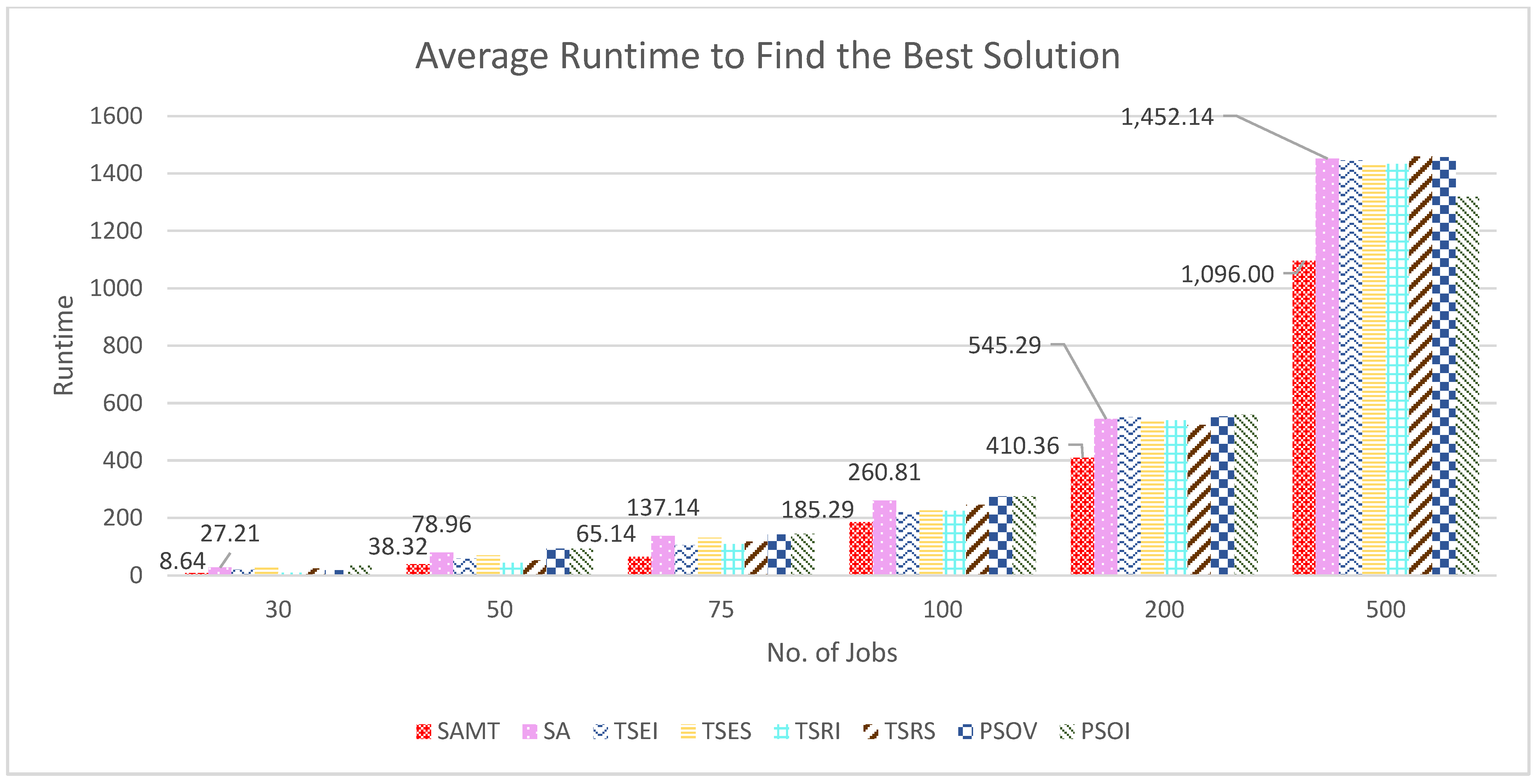
Apart from the robustness of the solution, the runtime to find the best OFV is another characteristic that should be assessed to determine the performance of the algorithms. Another two-way ANOVA table is established to understand whether there is a significant difference or not among the mean values of runtimes of the algorithms.
The ANOVA results in Table 6 reveal that at least one mean of the runtimes is not equal to the remaining means. Only Tukey’s HSD comparisons that are significantly different are listed in Table A6 of Appendix C, and the significant results from the Scheffe method are shown in Table A7.
The p-value of Tukey’s HSD test in Table A6 proves that the mean runtimes to find the best solution of the SA and SAMT algorithms are significantly different for problems with at least 50 jobs. The SAMT algorithm also provides a runtime advantage compared to all benchmark metaheuristics for problems with 200 and 500 jobs. Evaluating the results from the Scheffe method in Table A7 as a group suggests that SAMT can find the best OFV significantly more rapidly than SA, TSEI, PSOI, and PSOV for the problems that contain 200 jobs, as well as more rapidly than all algorithms in the case of the job number increasing to 500. According to Figure 6, it is possible to conclude that the SAMT algorithm needs a shorter runtime to find the best OV in comparison to the SA algorithm, thus yielding better or equal solutions. The SAMT algorithm provides better or equal objective function values in shorter run times compared to the SA algorithm.
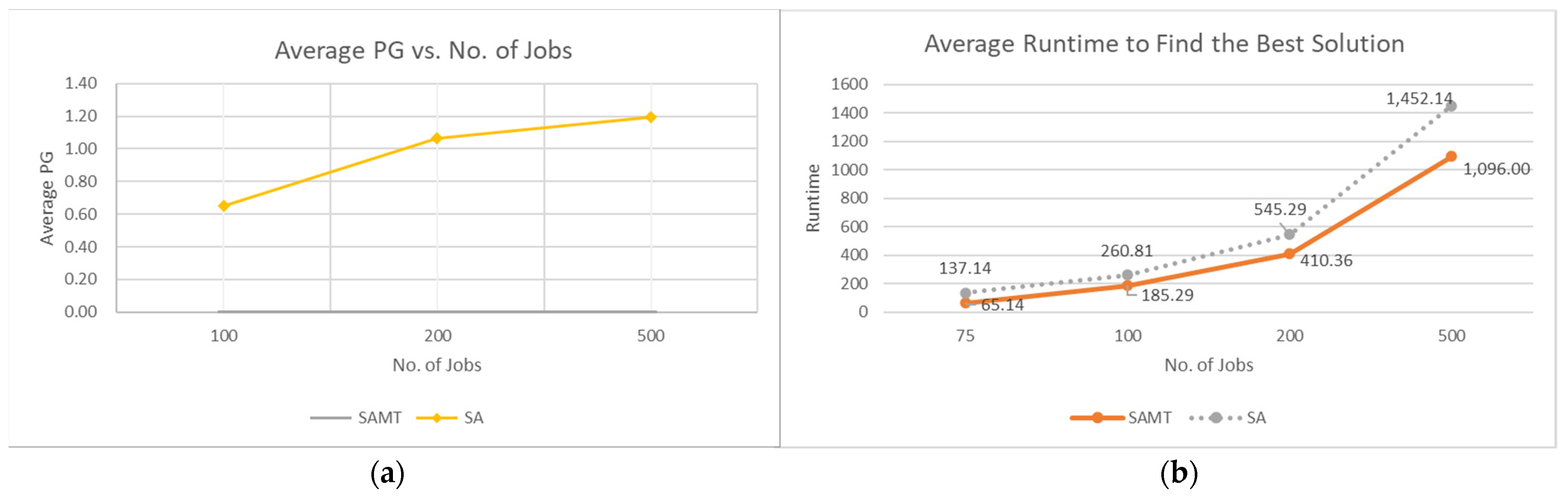
Figure 7 demonstrates the improvement by SAMT compared to the classical SA. The SAMT is compared to the average of two asynchronous runs of SA for being fair. In the case of GP, both Scheffe and Tukey’s HSD post hoc analysis suggests that SAMT is significantly better for the problems in the large-sized set. The PG increases nearly linearly while the number of jobs increases as seen in Figure 7a. Considering the runtime to find the best solution, Tukey’s HSD suggests that SAMT is better for problems with 75 or more jobs. The more conservative Scheffe method suggests that the number of jobs should be a minimum of 200 to derive significance. Figure 7b presents that the difference gradually increases with an exponential trend. The post hoc analysis and Figure 7 confirm that the proposed SAMT outperforms the classical SA in terms of both runtime and solution robustness, even if the SA runs two asynchronous threads and the better OFV of these threads is selected for comparison.
4. Discussion and Conclusions
In this paper, a novel parallel metaheuristic methodology named SAMT based on SA was proposed. The motivation of the study was to improve the poor runtime performance and search capability of the classical algorithm. In the methodology, a sub-thread runs in parallel to update the search direction of the main thread adaptively. The aim is to increase the capability of classical SA to find better solutions in shorter runtimes. The NWFSSP with earliness and tardiness objectives, , is considered for benchmarking. The literature review revealed that earliness and tardiness objectives for NWFSSP have not been widely studied. The most common practice to solve the research problem benefits from dispatching rules and heuristics. A major problem with dispatching rules and heuristics is their incapability to update themselves during runtime in contrast to metaheuristics. The study by Arabameri and Salmasi [18] was selected as the reference for benchmarking since the study included two important metaheuristic algorithms with different parameters.
The test runs and results of comparative analyses revealed that the SAMT algorithm could provide more robust solutions compared to the classical SA algorithm, variants of the PSO algorithms, and TS algorithms, whereby the solutions of the SAMT algorithm were slightly better in most cases of medium-sized problems and all cases of large-sized problems, even when the benchmark algorithms ran double asynchronous threads. Another contribution of this study was the enhancement of the runtime to provide a better solution in comparison to the SA algorithm. The SAMT algorithm consumed less time to find the best solution in large problems compared to benchmark problems. Unlike parallel computing, the proposed SAMT algorithm introduces independent parallel threads to enhance the robustness of the solution and overcome the runtime disadvantage of the classical SA algorithm. As intended, multiple threads of the SAMT algorithm grant a divergence–convergence strategy that enables the algorithm to explore the solution space more thoroughly and rapidly. The adaptive search strategy with a single slave thread is the novelty of this study. A temperature-dependent function stochastically determines the speed of the sub-thread at each run. Thus, the algorithm is adapted to jump into the solution space to decrease runtime and increase robustness.
The number of threads and parameters of the SA algorithm for each thread directly affected the performance of the SAMT algorithm. Hence, it is important to fine-tune each parameter systematically. An easy implementation for a single computer is through the FocusILS parameter tuning tool. The contribution of the study is the adaptive parameter tuning strategy of a single slave thread after analysis with the design of experiments (DOE). The purpose of the study was to present that the SA algorithm may be improved in terms of both time and result performance without excessive resource requirements, and the newly proposed algorithm is a robust methodology to solve the NWFSSP with the objective of addressing total earliness and tardiness. In future studies, the method may be enhanced by deploying it on multiple CPUs/GPUs with a distributed programming methodology. This method will be evaluated on different combinatorial optimization problems to confirm its efficiency. Another aspect will be to adapt different types of metaheuristics to a parallel methodology to solve the NWFSSP, before comparing them with the SAMT algorithm.
Author Contributions
Conceptualization, I.K., O.S. and S.B.; methodology, I.K., O.S. and S.B.; software, I.K.; validation, I.K. and O.S.; formal analysis, I.K. and O.S.; investigation, I.K.; resources, I.K.; data curation, I.K.; writing—original draft preparation, I.K.; writing—review and editing, O.S. and S.B.; visualization, I.K.; supervision, O.S. and S.B.; project administration, S.B. All authors have read and agreed to the published version of the manuscript.
Funding
The APC was funded by the company AN-EL Anahtar ve Elektrikli Ev Aletleri Sanayi A.S.
Institutional Review Board Statement
Not applicable.
Informed Consent Statement
Not applicable.
Data Availability Statement
Conflicts of Interest
The authors declare no conflict of interest. The funders had no role in the design of the study; in the collection, analyses, or interpretation of data; in the writing of the manuscript; or in the decision to publish the results.
Appendix A
This appendix includes the descriptions of benchmark algorithms.
Appendix A.1. Tabu Search (TS)
The TS algorithm was proposed by Glover [60] to solve integer programming problems. Furthermore, Glover et al. [61] published a user guide introducing perspectives for implementing TS on combinatorial or nonlinear problems. TS has been widely applied to scheduling problems. The algorithm iteratively improves the incumbent solution until the termination criteria are met. Short-term memory is utilized to restrict recent moves in the neighborhood to explore better solutions and avoid entrapment in local optima, while long-term memory helps to update the neighborhood dynamically to intensification [62]. Recent moves are added to the tabu list (TL) and restricted for a defined number of iterations. Considering the study by Arabameri and Salmasi [18], the size of the TL is determined according to Equation (A1).
An aspiration criterion should be defined to enable a better move to be confirmed even if it is in the tabu list. The aspiration criterion for this study is set as the objective value of the incumbent solution. Any move that has a better objective function than the current best solution is accepted regardless of the TL.
The TS algorithm is an incremental metaheuristic algorithm that iteratively updates an initial solution. Arabameri and Salmasi [18] evaluated three types of initial solution-creation mechanisms. Earliest due date (EDD) is the sequence in which the jobs are ordered according to their due dates in ascending order. The longest tardiness/earliness rate (LTER) rule considers the ratio of weights of earliness and tardiness, which are assumed to be “1” in this study. A random initial solution is formed with a sequence in which jobs are embedded in their positions randomly. Thus, two of these mechanisms are benchmarked in this study since LTER cannot grant an initial solution where all weights are equal to 1. Four combinations of TS algorithms are TS with the EDD initial solution and insertion neighborhood (TSEI), TS with a random initial solution and insertion neighborhood (TSRI), TS with the EDD initial solution and swap neighborhood (TSES), and TS with a random initial solution and swap neighborhood (TSRS). Until stopping criteria are met, a defined number of moves are carried out at each iteration, and the best move is selected as the new current solution if it is better than the current solution or meets the aspiration criteria. To improve the robustness of TS solutions, moves are compared at each iteration to balance the tradeoff between the number of moves at each iteration and the total number of iterations. The pseudocode of the TS algorithm is shown in Algorithm A1.
| Algorithm A1 Tabu Search |
| 1: Find the initial sequence by a construction heuristic or randomly |
| 2: Set the best sequence |
| 3: Set the current sequence |
| 4. Set tabu list |
| 5: Set = The maximum number of iterations |
| 6: Set |
| 7: While () |
| 8: Create the set as neighbor solutions of |
| 9: Find the best solution in the set |
| 10: If () |
| 11: If () |
| 12: Set |
| 13: Set |
| 14: If () |
| 15: Set |
| 16: Set |
| 17: Else |
| 18: If () (Aspiration) |
| 19: Set |
| 20: Set |
| 21: Set |
| 22: Set |
| 23: Set |
| 24: Do |
| 25: Return and |
Appendix A.2. Particle Swarm Optimization (PSO)
Kennedy and Eberhart [63] proposed the PSO algorithm as a social method to solve continuous nonlinear functions. The PSO algorithm is a population-based metaheuristic that iteratively updates its individuals. These individuals (namely, particles) represent solution instances that move with varying velocities and directions toward better solutions. The velocity and the direction of the particles are determined by the positions of both the global best solution and the best solution of the particle, the previous velocity, and the previous direction. The position of the i-th particle at the k-th iteration may be represented as where denotes its velocity.
The best position until the k-th iteration of a particle that is called p-best may be denoted as . The global best particle at the k-th iteration (namely, g-best) is demonstrated with the notation . The particles move toward p-best and g-best at each iteration to explore better solutions. Hence, the velocity of a particle may be updated according to Equation (A2) at each iteration as a function of the previous velocity, p-best, and g-best.
where is the up-to-date inertia weight that arranges the impact of the previous velocity, and are acceleration coefficients, and and are uniform random numbers from the interval . Upon calculation of , may be updated according to Equation (A3) at each iteration.
Being a powerful metaheuristic, the PSO algorithm also has drawbacks that limit convergence to the global best solution in some conditions. Commonly, the algorithm is trapped in local optima in high-dimensional spaces, and the rate of convergence is very low in the iterative process [64]. Hence, many improved, hybrid, or integrated versions have been suggested by researchers. In line with the study by Arabameri and Salmasi [18], the PSO algorithm is supported by integrating two different local search algorithms, insertion (PSOI) and variable neighborhood structure (PSOV). The flow of the PSOI algorithm is shown in Algorithm A2.
| Algorithm A2 PSOI Local Search |
| 1: Set the iteration number |
| 2: Set = The maximum number of iterations |
| 3: Calculate OFV for sequence |
| 4: While () |
| 5: Pick random integers and from the set |
| 6: Set a new sequence by executing on sequence |
| 7: Calculate OFV of sequence |
| 8: If () |
| 9: Set |
| 10: Set |
| 11: Set |
| 12: Do |
| 13: Return and |
The PSOI algorithm has a simple local search strategy that iteratively collates the solutions acquired by random moves with an insert operation and updates the incumbent solution to check if the new sequence returns a better OFV. The PSOV algorithm constitutes a relatively complex local search methodology. The pseudocode of the PSOV local search methodology is summarized in Algorithm A3. PSO-VNS attempts to discover better solutions by consulting insertion and swap operations sequentially. Upon perceiving a better OFV, the sub-interchange operation is executed to investigate the solution space further with the aim of improving the solution. The local search terminates after a defined number of maximum iterations.
| Algorithm A3 PSOV Local Search |
| 1: Set the iteration number |
| 2: Set = The maximum number of iterations |
| 3: Calculate OFV for sequence |
| 4: While () |
| 5: Pick random integers and from the set |
| 6: Set a new sequence by executing / on sequence |
| 7: Calculate OFV of sequence |
| 8: If () |
| 9: Set |
| 10: Set |
| 11: Set a new sequence by finding the best solution from |
| 12: on sequence |
| 13: Calculate OFV of sequence |
| 14: If () |
| 15: Set |
| 16: Set |
| 17: Else |
| 18: Set a new sequence by executing Swap / |
| 19: on sequence |
| 20: Calculate OFV of sequence |
| 21: If () |
| 22: Set |
| 23: Set |
| 24: Set |
| 25: Do |
| 26: Return and |
Appendix B
This appendix contains the results of the benchmark datasets. Table A1 shows the results of the Reeves dataset.

Table A1.
Results of Reeves dataset.
| Problem | Size | Minimum | SAMT | SA | TSEI | TSES | TSRI | TSRS | PSOV | PSOI |
|---|---|---|---|---|---|---|---|---|---|---|
| REC01-1 | 20 × 5 | 6044 | 0.00 | 0.00 | 0.00 | 0.00 | 0.00 | 0.00 | 0.00 | 0.00 |
| REC01-2 | 20 × 5 | 5113 | 0.00 | 0.00 | 0.00 | 0.00 | 0.00 | 0.00 | 0.00 | 0.00 |
| REC01-3 | 20 × 5 | 3567 | 0.00 | 0.00 | 0.00 | 0.00 | 0.00 | 0.00 | 0.00 | 0.00 |
| REC01-4 | 20 × 5 | 7412 | 0.00 | 0.00 | 0.00 | 0.00 | 0.00 | 0.00 | 0.00 | 0.00 |
| REC01-5 | 20 × 5 | 6904 | 0.00 | 0.00 | 0.00 | 0.00 | 0.00 | 0.00 | 0.00 | 0.00 |
| REC01-6 | 20 × 5 | 7124 | 0.00 | 0.00 | 0.00 | 0.00 | 0.00 | 0.00 | 0.00 | 0.00 |
| REC01-7 | 20 × 5 | 12,076 | 0.00 | 0.00 | 0.00 | 0.00 | 0.00 | 0.00 | 0.00 | 0.00 |
| REC07-1 | 20 × 10 | 7636 | 0.00 | 0.00 | 0.00 | 0.00 | 0.00 | 0.00 | 0.00 | 0.00 |
| REC07-2 | 20 × 10 | 6690 | 0.00 | 0.00 | 0.00 | 0.00 | 0.00 | 0.00 | 0.00 | 0.00 |
| REC07-3 | 20 × 10 | 5603 | 0.00 | 0.00 | 0.00 | 0.00 | 0.00 | 0.00 | 0.00 | 0.00 |
| REC07-4 | 20 × 10 | 11,882 | 0.00 | 0.00 | 0.00 | 0.00 | 0.00 | 0.00 | 0.00 | 0.00 |
| REC07-5 | 20 × 10 | 11,155 | 0.00 | 0.00 | 0.00 | 0.00 | 0.00 | 0.00 | 0.00 | 0.00 |
| REC07-6 | 20 × 10 | 13,542 | 0.00 | 0.00 | 0.00 | 0.00 | 0.00 | 0.00 | 0.00 | 0.00 |
| REC07-7 | 20 × 10 | 19,193 | 0.00 | 0.00 | 0.00 | 0.00 | 0.00 | 0.00 | 0.00 | 0.00 |
| REC13-1 | 20 × 15 | 9896 | 0.00 | 0.00 | 0.00 | 0.00 | 0.00 | 0.00 | 0.00 | 0.00 |
| REC13-2 | 20 × 15 | 9711 | 0.00 | 0.00 | 0.00 | 0.00 | 0.00 | 0.00 | 0.00 | 0.00 |
| REC13-3 | 20 × 15 | 9468 | 0.00 | 0.00 | 0.00 | 0.00 | 0.00 | 0.00 | 0.00 | 0.00 |
| REC13-4 | 20 × 15 | 16,141 | 0.00 | 0.00 | 0.00 | 0.00 | 0.00 | 0.00 | 0.00 | 0.00 |
| REC13-5 | 20 × 15 | 16,733 | 0.00 | 0.00 | 0.00 | 0.00 | 0.00 | 0.00 | 0.00 | 0.00 |
| REC13-6 | 20 × 15 | 15,970 | 0.00 | 0.00 | 0.00 | 0.00 | 0.00 | 0.00 | 0.00 | 0.00 |
| REC13-7 | 20 × 15 | 25,294 | 0.00 | 0.00 | 0.00 | 0.00 | 0.00 | 0.00 | 0.00 | 0.00 |
| REC19-1 | 30 × 10 | 17,490 | 0.00 | 0.00 | 0.00 | 0.00 | 0.00 | 0.00 | 0.00 | 0.00 |
| REC19-2 | 30 × 10 | 13,630 | 0.00 | 0.00 | 0.00 | 0.00 | 0.00 | 0.00 | 0.00 | 0.00 |
| REC19-3 | 30 × 10 | 11,977 | 0.00 | 0.00 | 0.00 | 0.00 | 0.00 | 0.13 | 0.00 | 0.00 |
| REC19-4 | 30 × 10 | 23,013 | 0.00 | 0.00 | 0.00 | 0.00 | 0.00 | 0.00 | 0.00 | 0.00 |
| REC19-5 | 30 × 10 | 20,592 | 0.00 | 0.00 | 0.00 | 0.00 | 0.00 | 0.00 | 0.00 | 0.00 |
| REC19-6 | 30 × 10 | 22,911 | 0.00 | 0.00 | 0.00 | 0.00 | 0.00 | 0.00 | 0.00 | 0.00 |
| REC19-7 | 30 × 10 | 38,065 | 0.00 | 0.00 | 0.00 | 0.00 | 0.00 | 0.00 | 0.00 | 0.00 |
| REC25-1 | 30 × 15 | 21,567 | 0.00 | 0.00 | 0.00 | 0.00 | 0.00 | 0.00 | 0.00 | 0.00 |
| REC25-2 | 30 × 15 | 19,609 | 0.00 | 0.00 | 0.00 | 0.13 | 0.00 | 0.00 | 0.00 | 0.00 |
| REC25-3 | 30 × 15 | 14,718 | 0.00 | 0.00 | 0.00 | 0.00 | 0.00 | 0.17 | 0.00 | 0.00 |
| REC25-4 | 30 × 15 | 31,156 | 0.00 | 0.00 | 0.00 | 0.00 | 0.00 | 0.00 | 0.00 | 0.00 |
| REC25-5 | 30 × 15 | 32,517 | 0.00 | 0.00 | 0.00 | 0.00 | 0.00 | 0.00 | 0.00 | 0.00 |
| REC25-6 | 30 × 15 | 30,218 | 0.00 | 0.00 | 0.00 | 0.00 | 0.00 | 0.00 | 0.00 | 0.00 |
| REC25-7 | 30 × 15 | 49,750 | 0.00 | 0.00 | 0.00 | 0.00 | 0.00 | 0.02 | 0.00 | 0.00 |
| REC31-1 | 50 × 10 | 41,984 | 0.00 | 0.00 | 0.00 | 0.00 | 0.00 | 0.01 | 0.00 | 0.00 |
| REC31-2 | 50 × 10 | 35,382 | 0.00 | 0.00 | 0.00 | 0.01 | 0.00 | 0.00 | 0.00 | 0.00 |
| REC31-3 | 50 × 10 | 28,949 | 0.00 | 0.00 | 0.00 | 0.00 | 0.00 | 0.00 | 0.00 | 0.00 |
| REC31-4 | 50 × 10 | 54,628 | 0.00 | 0.00 | 0.00 | 0.00 | 0.00 | 0.01 | 0.01 | 0.00 |
| REC31-5 | 50 × 10 | 47,261 | 0.00 | 0.00 | 0.00 | 0.00 | 0.00 | 0.00 | 0.00 | 0.00 |
| REC31-6 | 50 × 10 | 48,125 | 0.00 | 0.00 | 0.00 | 0.01 | 0.00 | 0.01 | 0.00 | 0.00 |
| REC31-7 | 50 × 10 | 84,550 | 0.00 | 0.00 | 0.00 | 0.00 | 0.00 | 0.00 | 0.00 | 0.00 |
| REC37-1 | 75 × 20 | 127,794 | 0.00 | 0.19 | 0.79 | 0.97 | 0.86 | 1.00 | 0.69 | 0.59 |
| REC37-2 | 75 × 20 | 107,509 | 0.00 | 0.25 | 0.79 | 0.93 | 0.86 | 0.79 | 0.64 | 0.64 |
| REC37-3 | 75 × 20 | 95,511 | 0.00 | 1.26 | 1.46 | 2.12 | 1.36 | 2.76 | 1.73 | 1.68 |
| REC37-4 | 75 × 20 | 174,195 | 0.00 | 0.23 | 1.22 | 1.50 | 1.20 | 1.21 | 0.42 | 0.24 |
| REC37-5 | 75 × 20 | 172,490 | 0.00 | 0.36 | 1.99 | 1.92 | 1.45 | 1.62 | 0.60 | 0.58 |
| REC37-6 | 75 × 20 | 158,079 | 0.00 | 0.11 | 1.25 | 1.51 | 0.83 | 1.14 | 0.36 | 0.33 |
| REC37-7 | 75 × 20 | 253,315 | 0.00 | 0.18 | 0.86 | 1.14 | 0.77 | 0.81 | 0.30 | 0.29 |
Table A2 presents the results of Taillard’s problems.
Table A2.
Results of Taillard dataset.
| Problem | Size | Minimum | SAMT | SA | TSEI | TSES | TSRI | TSRS | PSOV | PSOI |
|---|---|---|---|---|---|---|---|---|---|---|
| TAI001-1 | 20 × 5 | 5337 | 0.00 | 0.00 | 0.00 | 0.00 | 0.00 | 0.00 | 0.00 | 0.00 |
| TAI001-2 | 20 × 5 | 4097 | 0.00 | 0.00 | 0.00 | 0.00 | 0.00 | 0.00 | 0.00 | 0.00 |
| TAI001-3 | 20 × 5 | 2910 | 0.00 | 0.00 | 0.00 | 0.00 | 0.00 | 0.00 | 0.00 | 0.00 |
| TAI001-4 | 20 × 5 | 7118 | 0.00 | 0.00 | 0.00 | 0.00 | 0.00 | 0.00 | 0.00 | 0.00 |
| TAI001-5 | 20 × 5 | 6016 | 0.00 | 0.00 | 0.00 | 0.00 | 0.00 | 0.00 | 0.00 | 0.00 |
| TAI001-6 | 20 × 5 | 6219 | 0.00 | 0.00 | 0.00 | 0.00 | 0.00 | 0.00 | 0.00 | 0.00 |
| TAI001-7 | 20 × 5 | 11,210 | 0.00 | 0.00 | 0.00 | 0.00 | 0.00 | 0.00 | 0.00 | 0.00 |
| TAI011-1 | 20 × 10 | 8415 | 0.00 | 0.00 | 0.00 | 0.00 | 0.00 | 0.00 | 0.00 | 0.00 |
| TAI011-2 | 20 × 10 | 7553 | 0.00 | 0.00 | 0.00 | 0.00 | 0.00 | 0.00 | 0.00 | 0.00 |
| TAI011-3 | 20 × 10 | 6180 | 0.00 | 0.00 | 0.00 | 0.00 | 0.00 | 0.00 | 0.00 | 0.00 |
| TAI011-4 | 20 × 10 | 12,358 | 0.00 | 0.00 | 0.00 | 0.00 | 0.00 | 0.00 | 0.00 | 0.00 |
| TAI011-5 | 20 × 10 | 11,900 | 0.00 | 0.00 | 0.00 | 0.00 | 0.00 | 0.00 | 0.00 | 0.00 |
| TAI011-6 | 20 × 10 | 11,108 | 0.00 | 0.00 | 0.00 | 0.00 | 0.00 | 0.00 | 0.00 | 0.00 |
| TAI011-7 | 20 × 10 | 19,275 | 0.00 | 0.00 | 0.00 | 0.00 | 0.00 | 0.00 | 0.00 | 0.00 |
| TAI021-1 | 20 × 20 | 11,434 | 0.00 | 0.00 | 0.00 | 0.00 | 0.00 | 0.00 | 0.00 | 0.00 |
| TAI021-2 | 20 × 20 | 11,256 | 0.00 | 0.00 | 0.00 | 0.00 | 0.00 | 0.00 | 0.00 | 0.00 |
| TAI021-3 | 20 × 20 | 9593 | 0.00 | 0.00 | 0.00 | 0.00 | 0.00 | 0.00 | 0.00 | 0.00 |
| TAI021-4 | 20 × 20 | 19,362 | 0.00 | 0.00 | 0.00 | 0.00 | 0.00 | 0.00 | 0.00 | 0.00 |
| TAI021-5 | 20 × 20 | 19,276 | 0.00 | 0.00 | 0.00 | 0.00 | 0.00 | 0.00 | 0.00 | 0.00 |
| TAI021-6 | 20 × 20 | 21,420 | 0.00 | 0.00 | 0.00 | 0.00 | 0.00 | 0.00 | 0.00 | 0.00 |
| TAI021-7 | 20 × 20 | 31,878 | 0.00 | 0.00 | 0.00 | 0.00 | 0.00 | 0.00 | 0.00 | 0.00 |
| TAI031-1 | 50 × 5 | 29,891 | 0.00 | 0.20 | 1.13 | 2.44 | 1.37 | 4.24 | 0.00 | 0.73 |
| TAI031-2 | 50 × 5 | 24,332 | 0.00 | 0.00 | 0.52 | 4.63 | 1.37 | 2.34 | 0.35 | 0.44 |
| TAI031-3 | 50 × 5 | 15,589 | 0.00 | 0.00 | 0.81 | 0.53 | 0.00 | 4.64 | 0.80 | 1.81 |
| TAI031-4 | 50 × 5 | 31,761 | 0.00 | 0.00 | 0.00 | 0.13 | 1.10 | 1.32 | 0.00 | 0.00 |
| TAI031-5 | 50 × 5 | 26,324 | 0.00 | 0.04 | 0.81 | 0.77 | 2.70 | 5.89 | 0.61 | 0.00 |
| TAI031-6 | 50 × 5 | 17,286 | 0.00 | 0.00 | 0.92 | 5.94 | 0.75 | 1.45 | 0.00 | 0.00 |
| TAI031-7 | 50 × 5 | 53,175 | 0.00 | 0.19 | 0.35 | 0.43 | 1.14 | 1.41 | 0.41 | 0.26 |
| TAI041-1 | 50 × 10 | 43,470 | 0.00 | 0.36 | 0.90 | 1.19 | 0.55 | 4.29 | 0.73 | 0.42 |
| TAI041-2 | 50 × 10 | 35,949 | 0.00 | 0.00 | 0.00 | 0.66 | 0.10 | 0.41 | 0.22 | 0.61 |
| TAI041-3 | 50 × 10 | 26,059 | 0.00 | 0.00 | 0.41 | 1.67 | 0.00 | 0.92 | 0.31 | 0.00 |
| TAI041-4 | 50 × 10 | 55,980 | 0.00 | 0.63 | 1.74 | 1.75 | 0.45 | 1.04 | 0.80 | 0.52 |
| TAI041-5 | 50 × 10 | 51,615 | 0.00 | 0.09 | 0.32 | 1.00 | 0.46 | 1.28 | 0.03 | 0.09 |
| TAI041-6 | 50 × 10 | 50,136 | 0.00 | 0.07 | 1.50 | 0.45 | 1.69 | 2.85 | 0.08 | 0.46 |
| TAI041-7 | 50 × 10 | 86,223 | 0.00 | 0.00 | 0.72 | 0.85 | 0.97 | 1.04 | 0.00 | 0.00 |
| TAI051-1 | 50 × 20 | 69,200 | 0.00 | 0.24 | 0.27 | 0.32 | 0.22 | 0.77 | 0.33 | 0.23 |
| TAI051-2 | 50 × 20 | 58,340 | 0.00 | 0.21 | 0.42 | 0.84 | 0.97 | 0.68 | 0.29 | 0.39 |
| TAI051-3 | 50 × 20 | 51,722 | 0.00 | 0.53 | 0.92 | 1.34 | 0.50 | 0.80 | 0.72 | 0.82 |
| TAI051-4 | 50 × 20 | 92,524 | 0.00 | 0.22 | 0.93 | 0.75 | 0.43 | 0.78 | 0.32 | 0.29 |
| TAI051-5 | 50 × 20 | 95,055 | 0.00 | 0.34 | 1.03 | 1.69 | 0.54 | 1.55 | 0.30 | 0.49 |
| TAI051-6 | 50 × 20 | 89,895 | 0.00 | 0.00 | 1.21 | 1.22 | 0.13 | 2.34 | 0.58 | 0.87 |
| TAI051-7 | 50 × 20 | 140,138 | 0.00 | 0.06 | 0.71 | 1.16 | 1.01 | 0.99 | 0.15 | 0.50 |
| TAI061-1 | 100 × 5 | 129,568 | 0.00 | 0.74 | 0.42 | 1.92 | 1.63 | 1.24 | 0.83 | 0.37 |
| TAI061-2 | 100 × 5 | 99,123 | 0.00 | 0.94 | 1.86 | 2.22 | 1.21 | 3.74 | 1.14 | 1.05 |
| TAI061-3 | 100 × 5 | 66,640 | 0.00 | 0.25 | 4.62 | 3.34 | 2.04 | 3.02 | 0.78 | 1.62 |
| TAI061-4 | 100 × 5 | 134,753 | 0.00 | 0.74 | 1.40 | 1.48 | 1.97 | 2.75 | 1.35 | 1.52 |
| TAI061-5 | 100 × 5 | 111,145 | 0.00 | 0.53 | 3.01 | 2.46 | 1.21 | 1.88 | 0.87 | 0.78 |
| TAI061-6 | 100 × 5 | 88,702 | 0.00 | 0.85 | 1.99 | 4.14 | 2.27 | 5.32 | 1.34 | 0.53 |
| TAI061-7 | 100 × 5 | 210,576 | 0.00 | 0.47 | 0.93 | 1.20 | 1.13 | 1.47 | 0.74 | 0.71 |
| TAI071-1 | 100 × 10 | 167,093 | 0.00 | 0.28 | 0.52 | 0.94 | 0.71 | 1.60 | 0.36 | 0.35 |
| TAI071-2 | 100 × 10 | 126,832 | 0.00 | 0.64 | 0.82 | 1.19 | 1.24 | 2.29 | 0.58 | 0.94 |
| TAI071-3 | 100 × 10 | 94,769 | 0.00 | 0.87 | 0.91 | 3.37 | 1.32 | 2.30 | 0.49 | 0.94 |
| TAI071-4 | 100 × 10 | 200,061 | 0.00 | 0.37 | 1.33 | 1.58 | 0.96 | 1.58 | 0.87 | 0.77 |
| TAI071-5 | 100 × 10 | 177,140 | 0.00 | 0.46 | 1.91 | 1.38 | 0.82 | 1.09 | 0.94 | 0.62 |
| TAI071-6 | 100 × 10 | 164,182 | 0.00 | 0.66 | 1.96 | 3.28 | 2.05 | 2.92 | 0.74 | 0.99 |
| TAI071-7 | 100 × 10 | 306,976 | 0.00 | 1.12 | 1.02 | 2.18 | 2.50 | 3.59 | 0.92 | 1.10 |
| TAI081-1 | 100 × 20 | 237,085 | 0.00 | 0.56 | 1.31 | 1.84 | 0.82 | 1.57 | 0.49 | 0.97 |
| TAI081-2 | 100 × 20 | 215,998 | 0.00 | 0.87 | 1.06 | 2.31 | 1.84 | 1.53 | 1.24 | 1.30 |
| TAI081-3 | 100 × 20 | 186,009 | 0.00 | 0.49 | 1.32 | 2.12 | 1.61 | 3.60 | 0.89 | 1.21 |
| TAI081-4 | 100 × 20 | 313,809 | 0.00 | 0.75 | 1.26 | 1.44 | 1.42 | 2.16 | 0.82 | 1.23 |
| TAI081-5 | 100 × 20 | 300,851 | 0.00 | 0.27 | 1.29 | 2.28 | 0.73 | 2.46 | 0.48 | 0.88 |
| TAI081-6 | 100 × 20 | 310,201 | 0.00 | 0.80 | 2.15 | 2.91 | 3.03 | 3.07 | 1.54 | 1.13 |
| TAI081-7 | 100 × 20 | 442,923 | 0.00 | 1.02 | 1.94 | 2.34 | 1.94 | 2.51 | 1.08 | 1.15 |
| TAI091-1 | 200 × 10 | 629,975 | 0.00 | 0.63 | 2.30 | 2.82 | 1.78 | 3.19 | 1.37 | 1.26 |
| TAI091-2 | 200 × 10 | 491,187 | 0.00 | 0.96 | 2.06 | 0.53 | 2.13 | 1.11 | 1.30 | 1.54 |
| TAI091-3 | 200 × 10 | 375,423 | 0.00 | 0.83 | 3.47 | 2.51 | 2.68 | 2.06 | 1.76 | 2.13 |
| TAI091-4 | 200 × 10 | 737,822 | 0.00 | 1.25 | 1.89 | 2.53 | 1.88 | 2.74 | 2.07 | 1.75 |
| TAI091-5 | 200 × 10 | 650,818 | 0.00 | 1.42 | 1.87 | 2.47 | 2.15 | 2.24 | 1.62 | 1.87 |
| TAI091-6 | 200 × 10 | 579,224 | 0.00 | 0.98 | 3.17 | 2.76 | 2.55 | 2.92 | 1.87 | 1.76 |
| TAI091-7 | 200 × 10 | 1,105,327 | 0.00 | 0.70 | 2.37 | 1.77 | 1.88 | 1.31 | 1.32 | 1.27 |
| TAI101-1 | 200 × 20 | 893,397 | 0.00 | 0.41 | 1.20 | 1.14 | 1.19 | 0.94 | 0.80 | 1.14 |
| TAI101-2 | 200 × 20 | 773,905 | 0.00 | 1.75 | 2.76 | 3.04 | 2.58 | 3.39 | 1.95 | 2.35 |
| TAI101-3 | 200 × 20 | 655,942 | 0.00 | 1.08 | 2.33 | 3.02 | 2.56 | 2.42 | 1.62 | 1.52 |
| TAI101-4 | 200 × 20 | 1,124,882 | 0.00 | 0.57 | 2.28 | 2.20 | 2.03 | 2.24 | 1.23 | 1.26 |
| TAI101-5 | 200 × 20 | 1,054,993 | 0.00 | 1.80 | 3.53 | 3.00 | 3.24 | 3.67 | 2.64 | 2.36 |
| TAI101-6 | 200 × 20 | 1,000,185 | 0.00 | 1.64 | 1.34 | 2.73 | 2.40 | 3.92 | 2.47 | 2.77 |
| TAI101-7 | 200 × 20 | 1,589,543 | 0.00 | 0.93 | 1.65 | 1.93 | 1.70 | 2.11 | 1.28 | 1.34 |
| TAI111-1 | 500 × 20 | 5,577,501 | 0.00 | 0.69 | 1.80 | 2.88 | 1.84 | 4.07 | 1.62 | 1.64 |
| TAI111-2 | 500 × 20 | 4,773,182 | 0.00 | 1.26 | 2.24 | 3.42 | 2.29 | 4.53 | 2.21 | 2.23 |
| TAI111-3 | 500 × 20 | 4,037,988 | 0.00 | 2.20 | 3.20 | 4.29 | 3.24 | 5.45 | 3.20 | 3.17 |
| TAI111-4 | 500 × 20 | 6,817,377 | 0.00 | 1.52 | 2.55 | 3.63 | 2.54 | 4.71 | 2.55 | 2.54 |
| TAI111-5 | 500 × 20 | 6,535,252 | 0.00 | 1.92 | 2.97 | 4.03 | 2.97 | 5.30 | 2.93 | 2.95 |
| TAI111-6 | 500 × 20 | 6,092,434 | 0.00 | 0.56 | 1.65 | 2.70 | 1.66 | 4.02 | 1.60 | 1.62 |
| TAI111-7 | 500 × 20 | 9,449,083 | 0.00 | 0.21 | 1.23 | 2.28 | 1.25 | 3.47 | 1.22 | 1.23 |
Appendix C
The appendix contains the results of the post hoc analysis.
Table A3.
Tukey’s HSD results for algorithm × group for Group 2 considering PG.
| Algorithm | Group | Algorithm | Group | Difference | Lower | Upper | P Adj |
|---|---|---|---|---|---|---|---|
| PSOV | 2 | PSOI | 2 | −0.0168 | −0.3354 | 0.3018 | 1.0000 |
| SA | 2 | PSOI | 2 | −0.0831 | −0.4017 | 0.2355 | 1.0000 |
| SAMT | 2 | PSOI | 2 | −0.1462 | −0.4648 | 0.1724 | 0.9935 |
| TSEI | 2 | PSOI | 2 | 0.1173 | −0.2013 | 0.4359 | 0.9998 |
| TSES | 2 | PSOI | 2 | 0.2931 | −0.0254 | 0.6117 | 0.1221 |
| TSRI | 2 | PSOI | 2 | 0.1148 | −0.2038 | 0.4334 | 0.9998 |
| TSRS | 2 | PSOI | 2 | 0.4113 | 0.0927 | 0.7299 | 0.0007 |
| SA | 2 | PSOV | 2 | −0.0663 | −0.3849 | 0.2523 | 1.0000 |
| SAMT | 2 | PSOV | 2 | −0.1294 | −0.4480 | 0.1892 | 0.9989 |
| TSEI | 2 | PSOV | 2 | 0.1342 | −0.1844 | 0.4527 | 0.9980 |
| TSES | 2 | PSOV | 2 | 0.3100 | −0.0086 | 0.6286 | 0.0687 |
| TSRI | 2 | PSOV | 2 | 0.1317 | −0.1869 | 0.4503 | 0.9985 |
| TSRS | 2 | PSOV | 2 | 0.4281 | 0.1095 | 0.7467 | 0.0003 |
| SAMT | 2 | SA | 2 | −0.0631 | −0.3817 | 0.2555 | 1.0000 |
| TSEI | 2 | SA | 2 | 0.2005 | −0.1181 | 0.5190 | 0.8193 |
| TSES | 2 | SA | 2 | 0.3763 | 0.0577 | 0.6949 | 0.0042 |
| TSRI | 2 | SA | 2 | 0.1980 | −0.1206 | 0.5166 | 0.8358 |
| TSRS | 2 | SA | 2 | 0.4944 | 0.1758 | 0.8130 | 0.0000 |
| TSEI | 2 | SAMT | 2 | 0.2635 | −0.0551 | 0.5821 | 0.2864 |
| TSES | 2 | SAMT | 2 | 0.4393 | 0.1207 | 0.7579 | 0.0001 |
| TSRI | 2 | SAMT | 2 | 0.2610 | −0.0576 | 0.5796 | 0.3047 |
| TSRS | 2 | SAMT | 2 | 0.5575 | 0.2389 | 0.8761 | 0.0000 |
| TSES | 2 | TSEI | 2 | 0.1758 | −0.1428 | 0.4944 | 0.9434 |
| TSRI | 2 | TSEI | 2 | −0.0025 | −0.3211 | 0.3161 | 1.0000 |
| TSRS | 2 | TSEI | 2 | 0.2939 | −0.0247 | 0.6125 | 0.1190 |
| TSRI | 2 | TSES | 2 | −0.1783 | −0.4969 | 0.1403 | 0.9349 |
| TSRS | 2 | TSES | 2 | 0.1181 | −0.2005 | 0.4367 | 0.9997 |
| TSRS | 2 | TSRI | 2 | 0.2964 | −0.0222 | 0.6150 | 0.1097 |
Table A4.
Tukey’s HSD results for algorithm × group for Group 3 considering PG.
| Algorithm | Group | Algorithm | Group | Difference | Lower | Upper | P Adj |
|---|---|---|---|---|---|---|---|
| PSOV | 3 | PSOI | 3 | −0.0644 | −0.5334 | 0.4045 | 1.0000 |
| SA | 3 | PSOI | 3 | −0.5441 | −1.0130 | −0.0751 | 0.0057 |
| SAMT | 3 | PSOI | 3 | −1.4248 | −1.8937 | −0.9558 | 0.0000 |
| TSEI | 3 | PSOI | 3 | 0.5017 | 0.0327 | 0.9706 | 0.0206 |
| TSES | 3 | PSOI | 3 | 0.9945 | 0.5255 | 1.4634 | 0.0000 |
| TSRI | 3 | PSOI | 3 | 0.4557 | −0.0133 | 0.9247 | 0.0697 |
| TSRS | 3 | PSOI | 3 | 1.6113 | 1.1424 | 2.0803 | 0.0000 |
| SA | 3 | PSOV | 3 | −0.4796 | −0.9486 | −0.0107 | 0.0378 |
| SAMT | 3 | PSOV | 3 | −1.3603 | −1.8293 | −0.8914 | 0.0000 |
| TSEI | 3 | PSOV | 3 | 0.5661 | 0.0971 | 1.0351 | 0.0028 |
| TSES | 3 | PSOV | 3 | 1.0589 | 0.5899 | 1.5278 | 0.0000 |
| TSRI | 3 | PSOV | 3 | 0.5201 | 0.0512 | 0.9891 | 0.0120 |
| TSRS | 3 | PSOV | 3 | 1.6757 | 1.2068 | 2.1447 | 0.0000 |
| SAMT | 3 | SA | 3 | −0.8807 | −1.3496 | −0.4117 | 0.0000 |
| TSEI | 3 | SA | 3 | 1.0457 | 0.5768 | 1.5147 | 0.0000 |
| TSES | 3 | SA | 3 | 1.5385 | 1.0696 | 2.0075 | 0.0000 |
| TSRI | 3 | SA | 3 | 0.9998 | 0.5308 | 1.4687 | 0.0000 |
| TSRS | 3 | SA | 3 | 2.1554 | 1.6864 | 2.6244 | 0.0000 |
| TSEI | 3 | SAMT | 3 | 1.9264 | 1.4575 | 2.3954 | 0.0000 |
| TSES | 3 | SAMT | 3 | 2.4192 | 1.9502 | 2.8882 | 0.0000 |
| TSRI | 3 | SAMT | 3 | 1.8805 | 1.4115 | 2.3494 | 0.0000 |
| TSRS | 3 | SAMT | 3 | 3.0361 | 2.5671 | 3.5050 | 0.0000 |
| TSES | 3 | TSEI | 3 | 0.4928 | 0.0238 | 0.9618 | 0.0264 |
| TSRI | 3 | TSEI | 3 | −0.0460 | −0.5149 | 0.4230 | 1.0000 |
| TSRS | 3 | TSEI | 3 | 1.1097 | 0.6407 | 1.5786 | 0.0000 |
| TSRI | 3 | TSES | 3 | −0.5388 | −1.0077 | −0.0698 | 0.0067 |
| TSRS | 3 | TSES | 3 | 0.6169 | 0.1479 | 1.0858 | 0.0005 |
| TSRS | 3 | TSRI | 3 | 1.1556 | 0.6867 | 1.6246 | 0.0000 |
Table A5.
Scheffe method’s significant results for algorithm × group for GP.
| Algorithm | Group | Algorithm | Group | Difference | Lower | Upper | P Adj |
|---|---|---|---|---|---|---|---|
| TSRS | 2 | SAMT | 2 | 0.5575 | 0.0377 | 1.0772 | 0.0139 |
| SAMT | 3 | PSOI | 3 | −1.4248 | −2.1898 | −0.6597 | 0.0000 |
| TSES | 3 | PSOI | 3 | 0.9945 | 0.2294 | 1.7595 | 0.0001 |
| TSRS | 3 | PSOI | 3 | 1.6113 | 0.8463 | 2.3763 | 0.0000 |
| SAMT | 3 | PSOV | 3 | −1.3603 | −2.1253 | −0.5953 | 0.0000 |
| TSES | 3 | PSOV | 3 | 1.0589 | 0.2939 | 1.8239 | 0.0000 |
| TSRS | 3 | PSOV | 3 | 1.6757 | 0.9107 | 2.4408 | 0.0000 |
| SAMT | 3 | SA | 3 | −0.8807 | −1.6457 | −0.1157 | 0.0026 |
| TSEI | 3 | SA | 3 | 1.0457 | 0.2807 | 1.8107 | 0.0000 |
| TSES | 3 | SA | 3 | 1.5385 | 0.7735 | 2.3035 | 0.0000 |
| TSRI | 3 | SA | 3 | 0.9998 | 0.2348 | 1.7648 | 0.0000 |
| TSRS | 3 | SA | 3 | 2.1554 | 1.3904 | 2.9204 | 0.0000 |
| TSEI | 3 | SAMT | 3 | 1.9264 | 1.1614 | 2.6914 | 0.0000 |
| TSES | 3 | SAMT | 3 | 2.4192 | 1.6542 | 3.1842 | 0.0000 |
| TSRI | 3 | SAMT | 3 | 1.8805 | 1.1154 | 2.6455 | 0.0000 |
| TSRS | 3 | SAMT | 3 | 3.0361 | 2.2711 | 3.8011 | 0.0000 |
| TSRS | 3 | TSEI | 3 | 1.1097 | 0.3446 | 1.8747 | 0.0000 |
| TSRS | 3 | TSRI | 3 | 1.1556 | 0.3906 | 1.9206 | 0.0000 |
Table A6.
Tukey’s HSD results for algorithm × job considering time to find the best OFV.
| Algorithm | Jobs | Algorithm | Jobs | Difference | Lower | Upper | P Adj |
|---|---|---|---|---|---|---|---|
| SAMT | 50 | PSOI | 50 | −54.4286 | −89.8820 | −18.9752 | 0.0000 |
| TSRI | 50 | PSOI | 50 | −49.5000 | −84.9534 | −14.0466 | 0.0000 |
| TSRS | 50 | PSOI | 50 | −40.2500 | −75.7034 | −4.7966 | 0.0040 |
| SAMT | 50 | PSOV | 50 | −54.7500 | −90.2034 | −19.2966 | 0.0000 |
| TSRI | 50 | PSOV | 50 | −49.8214 | −85.2748 | −14.3680 | 0.0000 |
| TSRS | 50 | PSOV | 50 | −40.5714 | −76.0248 | −5.11802 | 0.0033 |
| SAMT | 50 | SA | 50 | −40.6429 | −76.0963 | −5.1895 | 0.0032 |
| TSRI | 50 | SA | 50 | −35.7143 | −71.1677 | −0.2609 | 0.0443 |
| SAMT | 75 | PSOI | 75 | −80.0000 | −150.9068 | −9.0932 | 0.0047 |
| SAMT | 75 | PSOV | 75 | −77.7143 | −148.6211 | −6.8075 | 0.0089 |
| SAMT | 75 | SA | 75 | −72.0000 | −142.9068 | −1.0932 | 0.0386 |
| SAMT | 100 | PSOI | 100 | −89.9048 | −130.8428 | −48.9667 | 0.0000 |
| TSEI | 100 | PSOI | 100 | −55.5714 | −96.5095 | −14.6334 | 0.0000 |
| TSES | 100 | PSOI | 100 | −49.0000 | −89.9381 | −8.0619 | 0.0011 |
| TSRI | 100 | PSOI | 100 | −50.0476 | −90.9857 | −9.1095 | 0.0006 |
| SAMT | 100 | PSOV | 100 | −90.5238 | −131.4619 | −49.5857 | 0.0000 |
| TSEI | 100 | PSOV | 100 | −56.1905 | −97.1285 | −15.2524 | 0.0000 |
| TSES | 100 | PSOV | 100 | −49.6190 | −90.5571 | −8.6810 | 0.0008 |
| TSRI | 100 | PSOV | 100 | −50.6667 | −91.6047 | −9.7286 | 0.0004 |
| SAMT | 100 | SA | 100 | −75.5238 | −116.4619 | −34.5857 | 0.0000 |
| TSEI | 100 | SA | 100 | −41.1905 | −82.1285 | −0.2524 | 0.0451 |
| TSRS | 100 | SAMT | 100 | 61.0000 | 20.0619 | 101.9381 | 0.0000 |
| SAMT | 200 | PSOI | 200 | −150.0000 | −200.1387 | −99.8613 | 0.0000 |
| SAMT | 200 | PSOV | 200 | −143.4286 | −193.5673 | −93.2899 | 0.0000 |
| SAMT | 200 | SA | 200 | −134.9286 | −185.0673 | −84.7899 | 0.0000 |
| TSEI | 200 | SAMT | 200 | 141.7857 | 91.6470 | 191.9244 | 0.0000 |
| TSES | 200 | SAMT | 200 | 128.4286 | 78.2899 | 178.5673 | 0.0000 |
| TSRI | 200 | SAMT | 200 | 129.7857 | 79.6470 | 179.9244 | 0.0000 |
| TSRS | 200 | SAMT | 200 | 114.0000 | 63.8613 | 164.1387 | 0.0000 |
| PSOV | 500 | PSOI | 500 | 138.4286 | 67.5218 | 209.3354 | 0.0000 |
| SA | 500 | PSOI | 500 | 133.4286 | 62.5218 | 204.3354 | 0.0000 |
| SAMT | 500 | PSOI | 500 | −222.7143 | −293.6211 | −151.8075 | 0.0000 |
| TSEI | 500 | PSOI | 500 | 127.4286 | 56.5218 | 198.3354 | 0.0000 |
| TSES | 500 | PSOI | 500 | 115.7143 | 44.8075 | 186.6211 | 0.0000 |
| TSRI | 500 | PSOI | 500 | 115.0000 | 44.0932 | 185.9068 | 0.0000 |
| TSRS | 500 | PSOI | 500 | 140.5714 | 69.6646 | 211.4782 | 0.0000 |
| SAMT | 500 | PSOV | 500 | −361.1429 | −432.0497 | −290.2360 | 0.0000 |
| SAMT | 500 | SA | 500 | −356.1429 | −427.0497 | −285.2360 | 0.0000 |
| TSEI | 500 | SAMT | 500 | 350.1429 | 279.2360 | 421.0497 | 0.0000 |
| TSES | 500 | SAMT | 500 | 338.4286 | 267.5218 | 409.3354 | 0.0000 |
| TSRI | 500 | SAMT | 500 | 337.7143 | 266.8075 | 408.6211 | 0.0000 |
| TSRS | 500 | SAMT | 500 | 363.2857 | 292.3789 | 434.1925 | 0.0000 |
Table A7.
Scheffe method’s significant results for algorithm × job considering time to find the best OFV.
Table A7.
Scheffe method’s significant results for algorithm × job considering time to find the best OFV.
| Algorithm | Group | Algorithm | Group | Difference | Lower | Upper | P Adj |
|---|---|---|---|---|---|---|---|
| SAMT | 200 | PSOI | 200 | −150.0000 | −284.9514 | −15.0486 | 0.0005 |
| SAMT | 200 | PSOV | 200 | −143.4286 | −278.3799 | −8.4772 | 0.0048 |
| SAMT | 200 | SA | 200 | −134.9286 | −269.8799 | 0.0228 | 0.0503 |
| TSEI | 200 | SAMT | 200 | 141.7857 | 6.8343 | 276.7371 | 0.0080 |
| SAMT | 500 | PSOI | 500 | −222.7143 | −413.5643 | −31.8642 | 0.0000 |
| SAMT | 500 | PSOV | 500 | −361.1429 | −551.9929 | −170.2928 | 0.0000 |
| SAMT | 500 | SA | 500 | −356.1429 | −546.9929 | −165.2928 | 0.0000 |
| TSEI | 500 | SAMT | 500 | 350.1429 | 159.2928 | 540.9929 | 0.0000 |
| TSES | 500 | SAMT | 500 | 338.4286 | 147.5785 | 529.2786 | 0.0000 |
| TSRI | 500 | SAMT | 500 | 337.7143 | 146.8642 | 528.5643 | 0.0000 |
| TSRS | 500 | SAMT | 500 | 363.2857 | 172.4357 | 554.1358 | 0.0000 |
References
- Pinedo, M. Scheduling; Springer: New York, NY, USA, 2012; Volume 29. [Google Scholar]
- Miyata, H.H.; Nagano, M.S.; Gupta, J.N. Integrating preventive maintenance activities to the no-wait flow shop scheduling problem with dependent-sequence setup times and makespan minimization. Comput. Ind. Eng. 2019, 135, 79–104. [Google Scholar] [CrossRef]
- Emmons, H.; Vairaktarakis, G. Flow Shop Scheduling: Theoretical Results, Algorithms, and Applications; Springer Science & Business Media: New York, NY, USA, 2012; Volume 182. [Google Scholar]
- Graham, R.L.; Lawler, E.L.; Lenstra, J.K.; Kan, A.H.G.R. Optimization and approximation in deterministic sequencing and scheduling: A survey. Ann. Discret. Math. 1979, 5, 287–326. [Google Scholar]
- Giaro, K. NP-hardness of compact scheduling in simplified open and flow shops. Eur. J. Oper. Res. 2001, 130, 90–98. [Google Scholar]
- Allahverdi, A. A survey of scheduling problems with no-wait in process. Eur. J. Oper. Res. 2016, 255, 665–686. [Google Scholar] [CrossRef]
- Aldowaisan, T.; Allahverdi, A. Minimizing total tardiness in no-wait flowshops. Found. Comput. Decis. Sci. 2012, 37, 149–162. [Google Scholar] [CrossRef]
- Liu, G.; Song, S.; Wu, C. Some heuristics for no-wait flowshops with total tardiness criterion. Comput. Oper. Res. 2013, 40, 521–525. [Google Scholar] [CrossRef]
- Ding, J.; Song, S.; Zhang, R.; Gupta, J.N.; Wu, C. Accelerated methods for total tardiness minimisation in no-wait flowshops. Int. J. Prod. Res. 2015, 53, 1002–1018. [Google Scholar] [CrossRef]
- Javadi, B.; Saidi-Mehrabad, M.; Haji, A.; Mahdavi, I.; Jolai, F.; Mahdavi-Amiri, N. No-wait flow shop scheduling using fuzzy multi-objective linear programming. J. Frankl. Inst. 2008, 345, 452–467. [Google Scholar]
- Tavakkoli-Moghaddam, R.; Rahimi-Vahed, A.R.; Mirzaei, A.H. Solving a multi-objective no-wait flow shop scheduling problem with an immune algorithm. Int. J. Adv. Manuf. Technol. 2008, 36, 969–981. [Google Scholar] [CrossRef]
- Abdollahpour, S.; Rezaian, J. Two new meta-heuristics for no-wait flexible flow shop scheduling problem with capacitated machines, mixed make-to-order and make-to-stock policy. Soft Comput. 2017, 21, 3147–3165. [Google Scholar] [CrossRef]
- Gao, F.; Liu, M.; Wang, J.-J.; Lu, Y.-Y. No-wait two-machine permutation flow shop scheduling problem with learning effect, common due date and controllable job processing times. Int. J. Prod. Res. 2018, 56, 2361–2369. [Google Scholar] [CrossRef]
- Li, Z.; Zhong, R.Y.; Barenji, A.V.; Liu, J.J.; Yu, C.X.; Huang, G.Q. Bi-objective hybrid flow shop scheduling with common due date. Oper. Res. 2021, 21, 1153–1178. [Google Scholar] [CrossRef]
- Lv, D.-Y.; Wang, J.-B. Study on resource-dependent no-wait flow shop scheduling with different due-window assignment and learning effects. Asia-Pac. J. Oper. Res. 2021, 38, 2150008. [Google Scholar] [CrossRef]
- Allali, K.; Aqil, S.; Belabid, J. Distributed no-wait flow shop problem with sequence dependent setup time: Optimization of makespan and maximum tardiness. Simul. Model. Pr. Theory 2022, 116, 102455. [Google Scholar] [CrossRef]
- Huang, R.-H.; Yang, C.-L.; Liu, S.-C. No-wait flexible flow shop scheduling with due windows. Math. Probl. Eng. 2015, 2015, 456719. [Google Scholar] [CrossRef]
- Arabameri, S.; Salmasi, N. Minimization of weighted earliness and tardiness for no-wait sequence-dependent setup times flowshop scheduling problem. Comput. Ind. Eng. 2013, 64, 902–916. [Google Scholar] [CrossRef]
- Schaller, J.; Valente, J.M. Minimizing total earliness and tardiness in a nowait flow shop. Int. J. Prod. Econ. 2020, 224, 107542. [Google Scholar] [CrossRef]
- Schaller, J.; Valente, J.M.S. Scheduling in a no-wait flow shop to minimise total earliness and tardiness with additional idle time allowed. Int. J. Prod. Res. 2022, 60, 5488–5504. [Google Scholar] [CrossRef]
- Guevara-Guevara, A.F.; Gómez-Fuentes, V.; Posos-Rodríguez, L.J.; Remolina-Gómez, N.; González-Neira, E.M. Earliness/tardiness minimization in a no-wait flow shop with sequence-dependent setup times. J. Proj. Manag. 2022, 7, 177–190. [Google Scholar] [CrossRef]
- Zhu, N.; Zhao, F.; Wang, L.; Ding, R.; Xu, T.; Jonrinaldi. A discrete learning fruit fly algorithm based on knowledge for the distributed no-wait flow shop scheduling with due windows. Expert Syst. Appl. 2022, 198, 116921. [Google Scholar] [CrossRef]
- Qian, B.; Zhang, Z.-Q.; Hu, R.; Jin, H.-P.; Yang, J.-B. A Matrix-Cube-Based Estimation of Distribution Algorithm for No-Wait Flow-Shop Scheduling With Sequence-Dependent Setup Times and Release Times. IEEE Trans. Syst. Man. Cybern. Syst. 2022, 1–12. [Google Scholar] [CrossRef]
- Ingber, L. Simulated annealing: Practice versus theory. Math. Comput. Model. 1993, 18, 29–57. [Google Scholar] [CrossRef]
- Greening, D.R. Simulated Annealing with Errors. Ph.D. Thesis, UCLA, California, LA, USA, 1995. [Google Scholar]
- Szu, H.; Hartley, R. Fast simulated annealing. Phys. Lett. A 1987, 122, 157–162. [Google Scholar] [CrossRef]
- Ingber, L. Very fast simulated re-annealing. Math. Comput. Model. 1989, 12, 967–973. [Google Scholar] [CrossRef]
- Malek, M.; Guruswamy, M.; Pandya, M.; Owens, H. Serial and parallel simulated annealing and tabu search algorithms for the traveling salesman problem. Ann. Oper. Res. 1989, 21, 59–84. [Google Scholar] [CrossRef]
- Yao, X. A new simulated annealing algorithm. Int. J. Comput. Math. 1995, 56, 161–168. [Google Scholar] [CrossRef]
- Roussel-Ragot, P.; Dreyfus, G. A problem independent parallel implementation of simulated annealing: Models and experiments. IEEE Trans. Comput. Des. Integr. Circuits Syst. 1990, 9, 827–835. [Google Scholar] [CrossRef]
- Mahfoud, S.W.; Goldberg, D.E. Parallel Recombinative simulated annealing: A genetic algorithm. Parallel Comput. 1995, 21, 1–28. [Google Scholar] [CrossRef]
- Lee, S.-Y.; Lee, K.G. Synchronous and asynchronous parallel simulated annealing with multiple Markov chains. IEEE Trans. Parallel Distrib. Syst. 1996, 7, 993–1008. [Google Scholar]
- Wodecki, M.; Bożzejko, W. Solving the flow shop problem by parallel simulated annealing. In International Conference on Parallel Processing and Applied Mathematics; Springer: Berlin/Heidelberg, Germany, 2001; pp. 236–244. [Google Scholar]
- Bożejko, W.; Wodecki, M. The new concepts in parallel simulated annealing method. In International Conference on Artificial Intelligence and Soft Computing; Springer: Berlin/Heidelberg, Germany, 2004; pp. 853–859. [Google Scholar]
- Czapiński, M. Parallel simulated annealing with genetic enhancement for flowshop problem with Csum. Comput. Ind. Eng. 2010, 59, 778–785. [Google Scholar] [CrossRef]
- Ferreiro, A.M.; García, J.A.; López-Salas, J.G.; Vázquez, C. An efficient implementation of parallel simulated annealing algorithm in GPUs. J. Glob. Optim. 2013, 57, 863–890. [Google Scholar] [CrossRef]
- Sonuc, E.; Sen, B.; Bayir, S. A parallel approach for solving 0/1 knapsack problem using simulated annealing algorithm on CUDA platform. Int. J. Comput. Sci. Inf. Secur. 2016, 14, 1096. [Google Scholar]
- Richie, J.E.; Ababei, C. Optimization of patch antennas via multithreaded simulated annealing based design exploration. J. Comput. Des. Eng. 2017, 4, 249–255. [Google Scholar] [CrossRef]
- Turan, H.H.; Kosanoglu, F.; Atmış, M. A multi-skilled workforce optimisation in maintenance logistics networks by multi-thread simulated annealing algorithms. Int. J. Prod. Res. 2021, 59, 2624–2646. [Google Scholar] [CrossRef]
- Vousden, M.; Bragg, G.M.; Brown, A.D. Asynchronous simulated annealing on the placement problem: A beneficial race condition. J. Parallel Distrib. Comput. 2022, 169, 242–251. [Google Scholar] [CrossRef]
- Zhou, X.; Ling, M.; Lin, Q.; Tang, S.; Wu, J.; Hu, H. Effectiveness Analysis of Multiple Initial States Simulated Annealing Algorithm, A Case Study on the Molecular Docking Tool AutoDock Vina. Available online: https://ssrn.com/abstract=4120348 (accessed on 19 December 2022).
- Coll, N.; Fort, M.; Saus, M. Coverage area maximization with parallel simulated annealing. Expert Syst. Appl. 2022, 202, 117185. [Google Scholar] [CrossRef]
- Yildirim, G. A novel hybrid multi-thread metaheuristic approach for fake news detection in social media. Appl. Intell. 2022, 1–21. [Google Scholar] [CrossRef]
- Deng, W.; Xu, J.; Song, Y.; Zhao, H. Differential evolution algorithm with wavelet basis function and optimal mutation strategy for complex optimization problem. Appl. Soft Comput. 2021, 100, 106724. [Google Scholar] [CrossRef]
- Cai, X.; Zhao, H.; Shang, S.; Zhou, Y.; Deng, W.; Chen, H.; Deng, W. An improved quantum-inspired cooperative co-evolution algorithm with muli-strategy and its application. Expert Syst. Appl. 2021, 171, 114629. [Google Scholar] [CrossRef]
- Valente, J.M.; Alves, R.A. Beam search algorithms for the early/tardy scheduling problem with release dates. J. Manuf. Syst. 2005, 24, 35–46. [Google Scholar] [CrossRef]
- Röck, H. The three-machine no-wait flow shop is NP-complete. J. ACM 1984, 31, 336–345. [Google Scholar] [CrossRef]
- Kirkpatrick, S.; Gelatt, C.D.; Vecchi, M.P. Optimization by simulated annealing. Science 1983, 220, 671–680. [Google Scholar] [CrossRef] [PubMed]
- Van Laarhoven, P.J.; Aarts, E.H. Simulated annealing. In Simulated Annealing: Theory and Applications; Springer: Dordrecht, The Netherlands, 1987; pp. 7–15. [Google Scholar]
- Nikolaev, A.G.; Jacobson, S.H. Simulated annealing. In Handbook of Metaheuristics; Springer: Boston, MA, USA, 2010; pp. 1–39. [Google Scholar]
- Bagherlou, H.; Ghaffari, A. A routing protocol for vehicular ad hoc networks using simulated annealing algorithm and neural networks. J. Supercomput. 2018, 74, 2528–2552. [Google Scholar] [CrossRef]
- Carlier, J. Ordonnancements à contraintes disjonctives. RAIRO Oper. Res. 1978, 12, 333–350. [Google Scholar] [CrossRef]
- Reeves, C.R. A genetic algorithm for flowshop sequencing. Comput. Oper. Res. 1995, 22, 5–13. [Google Scholar] [CrossRef]
- Amar, A.D.; Gupta, J.N.D. Simulated versus real life data in testing the efficiency of scheduling algorithms. IIE Trans. 1986, 18, 16–25. [Google Scholar] [CrossRef]
- Rinnooy Kan, A.H. Machine Scheduling Problems: Classification, Complexity, and Computations. Ph.D. Thesis, University of Amsterdam, Amsterdam, The Netherlands, 1976. [Google Scholar]
- Taillard, E. Benchmarks for basic scheduling problems. Eur. J. Oper. Res. 1993, 64, 278–285. [Google Scholar] [CrossRef]
- LaTorre, A.; Molina, D.; Osaba, E.; Poyatos, J.; Del Ser, J.; Herrera, F. A prescription of methodological guidelines for comparing bio-inspired optimization algorithms. Swarm Evol. Comput. 2021, 67, 100973. [Google Scholar] [CrossRef]
- Hutter, F.; Hoos, H.H.; Leyton-Brown, K.; Stuetzle, T. ParamILS: An automatic algorithm configuration framework. J. Artif. Intell. Res. 2009, 36, 267–306. [Google Scholar] [CrossRef]
- Lee, S.; Lee, D.K. What is the proper way to apply the multiple comparison test? Korean J. Anesthesiol. 2018, 71, 353–360. [Google Scholar] [CrossRef]
- Glover, F. Future paths for integer programming and links to artificial intelligence. Comput. Oper. Res. 1986, 13, 533–549. [Google Scholar] [CrossRef]
- Glover, F.; Taillard, E.; de Werra, D. A user’s guide to tabu search. Ann. Oper. Res. 1993, 41, 1–28. [Google Scholar] [CrossRef]
- Glover, F.; Laguna, M. Tabu search. In Handbook of Combinatorial Optimization; Springer: Boston, MA, USA, 1988; pp. 2093–2229. [Google Scholar]
- Kennedy, J.; Eberhart, R. Particle swarm optimization. In Proceedings of the ICNN’95-international Conference on Neural Networks. Perth, WA, Australia, 27 November–1 December 1995; Volume 4, pp. 1942–1948. [Google Scholar]
- Li, M.; Du, W.; Nian, F. An adaptive particle swarm optimization algorithm based on directed weighted complex network. Math. Probl. Eng. 2014, 2014, 434972. [Google Scholar] [CrossRef] [Green Version]
Figure 1.
Taxonomy of parallel simulated annealing methodologies [25].
Figure 1.
Taxonomy of parallel simulated annealing methodologies [25].

Figure 2.
Insert operation of Job 2 into Position 4.

Figure 3.
Swap operation of Job 2 and Job 4.

Figure 4.
Possible jumps by sub-threads on OFV curve.

Figure 5.
Average percentage gap vs. no. of jobs.

Figure 6.
Comparison of average runtimes to find the best solution.

Figure 7.
Average PG (a) and runtime to find the best solution (b). Comparison of SA and SAMT for significantly different cases.
Figure 7.
Average PG (a) and runtime to find the best solution (b). Comparison of SA and SAMT for significantly different cases.

Table 1.
Runtime limits considering the size of the problem.
| Problem Size | Runtime Limit (in s) |
|---|---|
| Small | |
| Medium | |
| Large |
Table 2.
The settings of the SAMT algorithm.
| Parameter | Value |
|---|---|
| : | Number of jobs |
| : | Following the total assigned runtime |
| : | 10 |
| : | 0.50 |
| : | |
| : | |
| : | |
| : | |
| : | 0.25 |
Table 3.
The settings of PSO algorithms.
| Variable/Parameter | Value/Formula |
|---|---|
| 2.05 | |
| 2.05 | |
| (PSOI) | |
| (PSOV) | 1.0 |
| (PSOI) | 30 |
| (PSOV) | 20 |
| Number of local search iterations |
Table 4.
Due date creation scheme.
| Index | TF | R |
|---|---|---|
| 1 | 0.20 | 0.20 |
| 2 | 0.20 | 0.50 |
| 3 | 0.20 | 0.80 |
| 4 | 0.50 | 0.20 |
| 5 | 0.50 | 0.50 |
| 6 | 0.50 | 0.80 |
| 7 | 0.80 | 0.20 |
Table 5.
ANOVA table for PG.
| Level | DoF | Sum of Sq. | Mean Sq. | F Value | Prob. (>F) |
|---|---|---|---|---|---|
| Algorithm | 7 | 115.8 | 16.54 | 47.57 | 0.0000 |
| Group | 2 | 581.3 | 290.65 | 835.75 | 0.0000 |
| Algorithm × group | 14 | 162.5 | 11.61 | 33.37 | 0.0000 |
| Residual | 1488 | 517.5 | 0.35 |
Table 6.
ANOVA table for runtime.
| Level | DoF | Sum of Sq. | Mean Sq. | F Value | Prob.(>F) |
|---|---|---|---|---|---|
| Algorithm | 7 | 277,595 | 39,656 | 42.9 | 0.0000 |
| Job | 13 | 123,270,879 | 9,482,375 | 10,258.8 | 0.0000 |
| Algorithm × job | 91 | 1,017,397 | 11,180 | 12.1 | 0.0000 |
| Residual | 1400 | 1,294,042 | 924 |
Disclaimer/Publisher’s Note: The statements, opinions and data contained in all publications are solely those of the individual author(s) and contributor(s) and not of MDPI and/or the editor(s). MDPI and/or the editor(s) disclaim responsibility for any injury to people or property resulting from any ideas, methods, instructions or products referred to in the content. |
© 2023 by the authors. Licensee MDPI, Basel, Switzerland. This article is an open access article distributed under the terms and conditions of the Creative Commons Attribution (CC BY) license (https://creativecommons.org/licenses/by/4.0/).
Share and Cite
MDPI and ACS Style
Karacan, I.; Senvar, O.; Bulkan, S. A Novel Parallel Simulated Annealing Methodology to Solve the No-Wait Flow Shop Scheduling Problem with Earliness and Tardiness Objectives. Processes 2023, 11, 454. https://doi.org/10.3390/pr11020454
AMA Style
Karacan I, Senvar O, Bulkan S. A Novel Parallel Simulated Annealing Methodology to Solve the No-Wait Flow Shop Scheduling Problem with Earliness and Tardiness Objectives. Processes. 2023; 11(2):454. https://doi.org/10.3390/pr11020454
Chicago/Turabian StyleKaracan, Ismet, Ozlem Senvar, and Serol Bulkan. 2023. "A Novel Parallel Simulated Annealing Methodology to Solve the No-Wait Flow Shop Scheduling Problem with Earliness and Tardiness Objectives" Processes 11, no. 2: 454. https://doi.org/10.3390/pr11020454
Note that from the first issue of 2016, this journal uses article numbers instead of page numbers. See further details here.