
A GAPN Approach for the Flexible Job-Shop Scheduling Problem with Indirect Energy and Time-of-Use Electricity Pricing


1
School of Computer Science, Guangdong Polytechnic Normal University, Guangzhou 510665, China
2
School of Economics and Management, Guangdong Technology College, Zhaoqing 526070, China
3
School of Cyber Security, Guangdong Polytechnic Normal University, Guangzhou 510665, China
*
Author to whom correspondence should be addressed.
Processes 2022, 10(5), 832; https://doi.org/10.3390/pr10050832
Submission received: 21 March 2022
/
Revised: 18 April 2022
/
Accepted: 19 April 2022
/
Published: 22 April 2022
(This article belongs to the Special Issue Green Manufacturing and Low-Carbon Control of Mechanical and Electrical Products)
Abstract
:The flexible job-shop scheduling problem with indirect energy and time-of-use (ToU) electricity pricing (FJSP-IT) is investigated. Considering the production cost, which includes the indirect energy cost, direct energy cost and time cost, the cost evaluation model under ToU pricing is built. To minimize the total production cost of the FJSP-IT, an approach based on a genetic algorithm and Petri nets (GAPN) is presented. Under this approach, indirect energy and direct energy are modeled with Petri net (PN) nodes, the operation time is evaluated through PN simulation, and resource allocation is fine-tuned through genetic operations. A group of heuristic operation time policies, especially the exhausting subsection policy and two mixed policies, are presented to adapt to the FJSP-IT with vague cost components. Experiments were performed on a data set generated from the banburying shop of a rubber tire plant, and the results show that the proposed GAPN approach has good convergence. Using the proposed operation time policies makes it possible to save 10.81% on the production cost compared to using the single off-peak first or passive delay policy, and considering indirect energy makes it possible to save at least 2.09% on the production cost compared to ignoring indirect energy.
1. Introduction
With global warming and fossil fuel depletion, time-of-use (ToU) pricing, in which higher electricity prices are charged during on-peak hours and considerably lower prices are charged otherwise, has been widely adopted to encourage plants to avoid on-peak power generated by fossil fuels. Currently, ToU pricing has become a key factor in production scheduling for energy-intensive manufacturing enterprises to save on the production cost [1,2,3,4]. The flexible job-shop scheduling problem (FJSP) is a classical production scheduling problem that allows an operation to be processed by any machine from a given set. A few extended FJSPs with ToU pricing have recently been presented to save on the production cost. Zhang et al. [5] extended the objective of the FJSP by considering the tardiness cost, direct energy cost and auxiliary energy cost under ToU pricing. They established an electricity cost model with ToU pricing by dividing the energetic status of machines into waiting, setup and process, and proposed a parallel gene expression programming approach to minimize the total production cost. Far et al. [6] extended some limitations on entire energy consumption, total manufactured emission and part defect percentage, and presented a self-adaptive two-phase subpopulation genetic algorithm to find a near-optimum solution of total cost and total delivery tardiness. Moon and Park [7], Hadera et al. [8] and Hadera et al. [9] presented FJSPs with generators and energy storage systems under ToU pricing. They tried to minimize the electricity cost by scheduling processing activities together with charging/discharging and generating activities. Du et al. [10] presented an extended FJSP with splitting and recombining activities. They established a biobjective (production delay and energy cost under ToU pricing) mathematical model and found Pareto-optimal solutions using an improved nondominated sorting genetic algorithm version II (NSGA-II). However, few FJSPs with ToU pricing take into account indirect energy and the operation time policy.
Indirect energy is the energy consumed by nonprocessing activities (lighting, heating, ventilation, etc.) to maintain the manufacturing environment [11]. It is considerable, especially in plants that need heating, ventilation and air conditioning (HVAC) to maintain a production environment, e.g., some chemical and food plants. Indirect energy is separated from production energy consumption, as well as theoretical energy and auxiliary energy. Theoretical energy is the minimum energy required to carry out processes, whereas auxiliary energy is the energy required by the supporting activities and auxiliary equipment for the processes. Indirect energy and auxiliary energy are regarded as non-value-added and should be minimized in production scheduling [11]. Liang et al. [12] considered the indirect energy incurred by stock in a single machine environment and suggested minimizing the production cost through processing technology selection. Auxiliary energy, including the stand-by, idle and the setup energy of a machine, is seriously considered in many production scheduling problems [5,13,14,15,16,17,18,19], but indirect energy is almost ignored in the FJSP due to the difficulty of cost evaluation with complex constraints.
The operation time is a class of key decision variables for production scheduling to minimize the production cost under ToU pricing. At present, studies on the operation time policy under ToU pricing are mostly designed for single and parallel machine scheduling problems, in which the delay cost is relatively easy to evaluate. These policies can be summarized into three classes: passive delay, off-peak first and the highest density first. Passive delay policies do not take the operation time as a decision variable, and they reduce production by seeking the optimal resource allocation and operation order. Their main extension is the production cost objective under ToU pricing. Most energy-aware FJSPs adopt passive delay policies (see [1,3,5,7,20,21]). Off-peak first policies attempt to put operations in off-peak periods and avoid on-peak periods. They are very prevalent in daily production practice due to their simplicity. Undoubtedly, passive delay policies are effective for time cost-intensive shop scheduling, whereas off-peak period policies are effective for energy-intensive shop scheduling. However, for shops with vague cost components, the two classes of policies may be unable to trade-off between the delay cost and the electricity cost.
The highest density first policy was first proposed for a single machine scheduling model in [3,22]. It first schedules high-power jobs in off-peak periods and then inserts other jobs in free periods. Some studies have suggested expanding its application scope by converting complex scheduling problems into single machine scheduling problems, and subsequently, the policy has been improved for unrelated parallel machine scheduling [23,24,25], flow job shop scheduling [26] and batch scheduling [27,28,29,30]. The highest density first policy can be regarded as a mixture of the off-peak first policy and passive delay policy, but it lacks self-adaptability to variable production cost components and can cover only a limited problem space. Due to complex operation sequence constraints and shared resource constraints, it is very difficult to convert the FJSP into single and parallel machine scheduling problems for which the highest density first policy can be applicable. Moreover, considering indirect energy makes the relation between the time cost and the electricity cost very uncertain. Novel operation time policies need to be presented to trade off the delay cost and the electricity cost.
From the literature review above, two study limitations can be found: (1) indirect energy is not seriously considered in the FJSP; (2) the operation time policy under ToU pricing is not sufficiently studied for the FJSP. Therefore, this study investigates the FJSP with indirect energy and ToU pricing (FJSP-IT), in which indirect energy is considerable and ToU pricing is adopted, hence, operation time policies should be suggested.
The FJSP is well-known as a class of models with high complexity due to routing flexibility and shared resources. Petri nets (PNs) have demonstrated that they are able to model FJSPs with numerous contributions, such as concurrent and asynchronous activities, resource sharing, routing flexibility and complex sequence constraints. The major advantages of using PNs in production scheduling systems over formulas include the ability to represent multiple states in a concise manner, to capture precedence relations and structural interactions, and to model deadlocks, conflicts, buffer sizes, and multiresource constraints [31,32,33,34].
A variety of PN subclasses have been developed for modeling the FJSP. Ezpeleta et al. [35] defined a classical PN subclass called Systems of Simple Sequential Processes with Resources (S3PR), in which each job is modeled with a subnet composed of a number of serial processes and the subnets are linked through resource capacity constraints. Barkaoui and Abdallah [36] extended S3PR to Systems of Sequential Systems with Shared Resources (S4R), in which one resource can be allocated to multiple concurrent processes. Mejia et al. [37] defined a PN subclass called Set of Simple Open Processes with Resources (S2OPR) for the FJSP with full routing flexibility. These PNs can effectively formalize the sequence and resource constraints of the FJSP, but ignore the processing time, and subsequently, many works have used the time Petri net (TPN) to compensate for the capability of modeling the process time. Based on the time property adopted in PNs, the TPN primarily includes the place-timed PN [32,38,39,40] and the transition-timed PN [41,42,43], and the delay time is associated with the place and the transition, respectively. Energy and material consumption have also been associated with the place and the transition as well as the delay time in [41,44,45,46,47]. Nonetheless, indirect energy has not been modeled in the abovementioned PNs.
The operation time policies are part of the solving approach for the FJSP-IT and should be integrated into a solving framework. In general, an FJSP can be decomposed into resource allocation and operation sequences, and it is solved using a genetic algorithm (GA) [13,48], an ant optimization algorithm [15], a heuristic algorithm [5], etc. The genetic algorithm and Petri nets (GAPN) are classical approaches for solving FJSPs. In GAPN, a solution is encoded by a route composed of places and transitions, and objectives are evaluated by simulating PNs. It is concluded in [39,49], that the GAPN is an approach that provides good performance in reasonable computer times, and at the same time, can be adapted to real settings where many constraints, such as multiplicity of resources, recirculation and assembly operations, are not traditionally handled by classical algorithms, such as linear and mixed integer programming, branch and bound or dynamic programming. Thus, the GAPN provides feasible guidance for modeling the indirect energy within PNs and evaluating the effect of operation time policies through PN simulation.
Based on the review of the related literature, there is no approach in which the FJSP-IT can optimize the operation time together with resource allocation. To solve the FJSP-IT, three difficulties need to be overcome. First, indirect energy together with ToU pricing enhances the complexity of the relation between the energy cost and operation time and becomes a decision difficulty. Second, indirect energy enhances the complexity of modelling the problem since a new type of cost should be introduced in the objective and decision. Third, the operation time needs to be optimized together with resource allocation, which enhances the complexity of the solving approach.
To overcome these difficulties, a GAPN approach for the FJSP-IT is presented in this paper. The main contributions of this paper rely on three main suggestions to minimize the production cost: a group of operation time policies, a PN model that formalizes indirect energy and a GAPN framework allowing resource allocation along with operation time decisions. The operation time policies include the exhausting subsection policy and two mixed policies and adapt to the FJSP-IT with vague cost components. The PN model embeds indirect energy in sequence and shared resource constraints and enables the simulation of the production cost with the operation time. The GAPN framework integrates the operation time decision with the resource allocation decision and decomposes the complexity of the solution to FJSP-IT.
The rest of this paper is organized as follows. Section 2 defines the FJSP-IT. Section 3 presents the PN model with indirect energy. Section 4 presents the GAPN approach for the FJSP-IT, including operation time policies, the PN simulation algorithm and the GA for optimization. Computational experiments and result analysis are conducted in Section 5. Conclusions are drawn in Section 6.
2. Problem Definition
2.1. Concepts and Assumptions
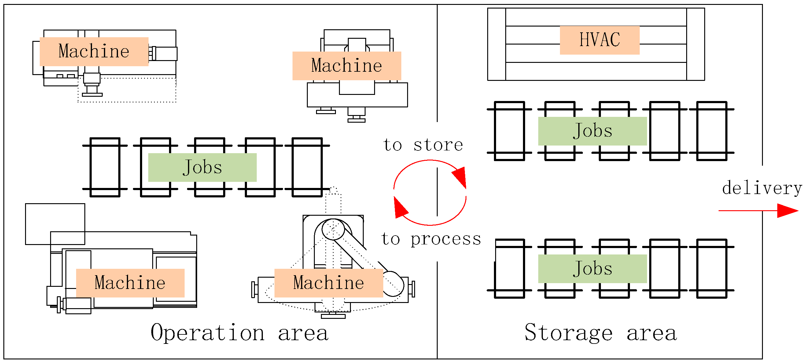
Observing some processes of chemical shops and food shops, it is found that storage between two operations is usually necessary to wait for cooling or chemical reactions, and storage areas usually need HVAC to maintain the environment. Thus, we generalize a flexible manufacturing system with storage between two operations, as shown in Figure 1. A job shop is separated into an operation area and a storage area. A job needs to be stored in a storage area for a given time between two operations or before delivery. The considerable storage energy is just indirect energy.
The following notations will be used for problem definition throughout the paper.
| Indices and sets | |
| J | The set of jobs |
| Jj | The jth individual job, Jj∈J |
| R | The set of machine resources |
| Ri | The ith individual machine, Ri∈R |
| O | The set of operations |
| Oj | The subset of operations of job Jj, Oj⊆O |
| Oj,k | The kth operation of job Jj, Oj,k∈Oj |
| Xj,k,i | The possible execution in which operation Oj,k can be executed by machine Ri |
| Xj,k | The subset of executions for operation Oj,k, Xj,k,i∈Xj,k, and an operation can be executed by more than one machine |
| X | The set of executions for job set J, Xj,k⊆X |
| S | The set of storages |
| Sj,k | The storage after operation Oj,k |
| L | The set of price periods under ToU pricing |
| Ll | The lth price periods under ToU pricing, Ll∈L |
| Parameters | |
| d | The delivery time of job set J |
| tm(x) | The time consumption of an execution (or storage), x∈X∪S |
| pwr(x) | The power consumption of an execution (or storage), x∈X∪S |
| tm’(s) | The actual time consumption of a storage, tm’(s) ≥tm(x) |
| K | The time cost per hour |
| el | The electricity price of period Ll |
| tm(x,l) | The time consumption of execution x in period Ll, x∈X |
| tm’(s,l) | The actual time consumption of storage s in period Ll, s∈S |
| Decision variables | |
| allocate(o) | The resource allocation to operation o, o∈O, allocate(Oj,k)∈Xj,k |
| start(o) | The operation time (also the start time) of o, o∈O |
| Ra | The set of resource allocations to all operations, ={ allocate(o)| o∈O } |
| St | The set of operation times, ={start(o)| o∈O } |
| Sv | The solution to a FJSP-IT, =(Ra, St) |
| Objective variables | |
| PC(Sv) | The production cost of a solution |
| TC(Sv) | The time cost of a solution |
| EC(Sv) | The energy cost of a solution |
A generic FJSP can be viewed as a set of n jobs to be processed on a set of m machines . Each job Jj consists of a predetermined sequence of (hj) operations that can be executed by more than one machine [38,39,49].
In this paper, we assume that the production in the operation area is a generic flexible production system and that the main extension in the FJSP-IT is the storage following each operation. Hence, each job Jj in a FJSP-IT has storages . Each storage time must be longer than a given time; its actual value is the interval between two adjacent operations. tm(Sj,k) denotes the given time of storage Sj,k and tm’(Sj,k) denotes the actual time of storage Sj,k. The electricity price is ToU pricing, and only power energy is considered in the energy cost since the other types of energy are independent of ToU pricing. Auxiliary energy is not separately considered since it has been carefully studied in many works. In this study, the electricity consumed by operations is considered direct energy and the electricity consumed by storages is considered indirect energy.
Other assumptions of the FJSP-IT are as follows:
- (1)
- All machines are available at a given start time;
- (2)
- All jobs are released at a given start time;
- (3)
- All jobs are independent of each other;
- (4)
- All jobs are delivered together as soon as they are ready;
- (5)
- Each machine can execute only one operation at a time;
- (6)
- Each operation can be executed without interruption;
- (7)
- The order of operations for each job is predefined and cannot be modified;
- (8)
- The energy consumption of each machine is zero without execution;
- (9)
- ToU pricing sets different hourly electricity prices in one day;
- (10)
- The time cost per hour is a constant K.
2.2. Objective and Decision
From the demand-side perspective, the objective of an FJSP-IT is to minimize PC(Sv). Based on the abovementioned concepts and assumptions, the decision of the FJSP-IT involves selecting a machine and choosing an operation time for each operation to meet the objective. Formally, the decision involves determining allocate(o) and start(o). Hence, one solution of an FJSP-IT can be represented by a set of resource allocations and operation times, represented as Sv = (Ra, St). Storage is not included in a solution because it is unnecessary for allocating machines and choosing operation times; it is used only to evaluate the indirect energy cost. A solution must satisfy the complex sequence and shared resource constraints, which will be formalized by PNs instead of formulas.
2.3. Production Cost Evaluation
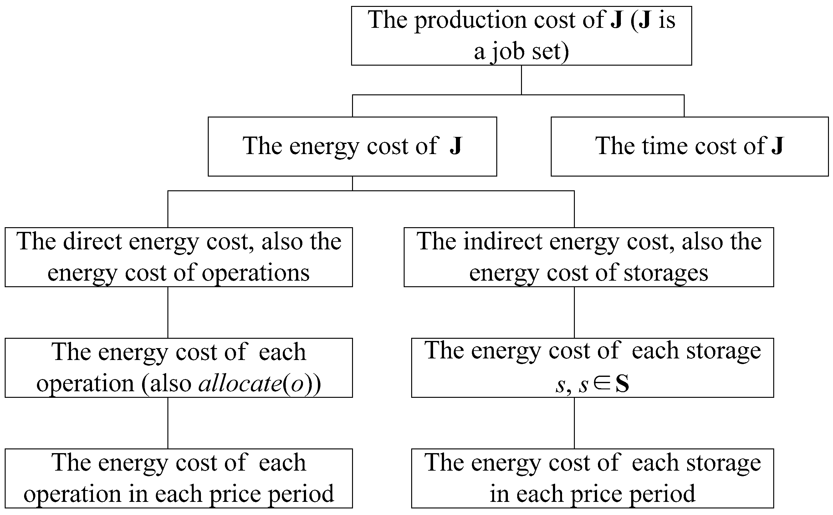
Given a feasible solution Sv = (Ra, St), the production cost can be evaluated based on the parameters of the FJSP-IT. We establish a breakdown model to evaluate the production cost of the FJSP-IT. The production cost is broken down into the energy cost and the time cost and, furthermore, the energy cost is broken down from the perspective of the job set, direct/indirect energy, the individual job and the price period. The breakdown model is represented as Figure 2.
The breakdown of the top three levels is represented as Equations (1) and (2):
where EC(O) denotes the direct energy cost consumed by operations and EC(S) denotes the indirect energy cost consumed by storages.
PC(Sv) = EC(Sv) + TC(Sv)
EC(Sv) = EC(O) + EC(S)
EC(O) and EC(S) are broken down into the cost of individual jobs and furthermore into the cost of individual operations and storages. The two breakdowns are represented as Equations (3) and (4):
and are broken down into the energy cost in ToU pricing periods. The two breakdowns are represented as Equations (5) and (6):
where depends on start(Oj,k), tm(Oj,k) and price period Ll.
where tm’(Sj,k) is the actual time consumption of Sj,k, depends on start(Oj,k+1), start(Oj,k) and price period Ll, and is represented as Equation (7).
According to the assumption that all jobs are delivered together as soon as they are ready, d, the delivery time of job set J can be evaluated by Equation (8):
TC(J) is represented as Equation (9):
3. Petri Net Modeling
3.1. Basic Definition of PNs
A PN is a bipartite, weighted, directed graph composed of places, transitions and arcs that connect the place and the transition, either from the transition to the place or vice versa [50]. It can be represented by a five-tuple , where P and T denote the finite and disjoint sets of places and transitions, respectively, P∩T = ∅, P ≠ ∅, T ≠ ∅. F refers to the set of directed arcs, F⊆(P × T)∪(T × P). W is the weighting function and M0 is the initial marking. A k-weighted arc can be regarded as k parallel unit arcs and the label of the unit arc is generally omitted. The marking or state of PN can be denoted by M = [M(p1), M(p2), …, M(pv)], where the vth element M(pv) means the number of tokens in the pv place. For t∈T, ·t(t) means the set of pre-places (post-places) of transition t. For p∈P,·p(p) means the set of pre-transitions (post-transitions) of place p. A transition t∈T is enabled or fireable if ∀p∈·t: M(p) ≥ w(p, t). M[t> denotes the t is fired and w(p, t) denotes the weight of the directed arc from p to t. Similarly, w(t, p) means the weight of the arc from t to p. Firing an enabled transition will result in the generation of reachable marking M′ from marking M, which can be represented as M[t>M′. The successive marking M′ can be determined by Equation (10) [41]:
A TPN is a class of extended PNs in which places or transitions are associated with a time property. It can be represented by a five-tuple , where τ denotes the extended time property [42].
3.2. Transition-Timed PN for the FJSP-IT
According to the definition of the FJSP-IT, storage and power need to be modeled by a PN as well as the operation and time. Since the transition-timed PN is more advantageous than the position-timed PN in preventing deadlock [44], an FJSP-IT will be modeled on the basis of the transition-timed PN, in which executions and storages are modeled with transitions. Therefore, the τ of a TPN for the FJSP-IT is extended as a triple τ = (pwr, tm, act), where pwr(t) denotes the power consumption of transition t, tm(t) denotes the time consumption of transition t and act(t) denotes the activeness of transition t. The property act is a Boolean type, where true denotes that the associated transition can be triggered by delay, whereas false denotes the opposite. Correspondingly, the transition with true act indicates an active transition, and that with false act indicates a passive transition.
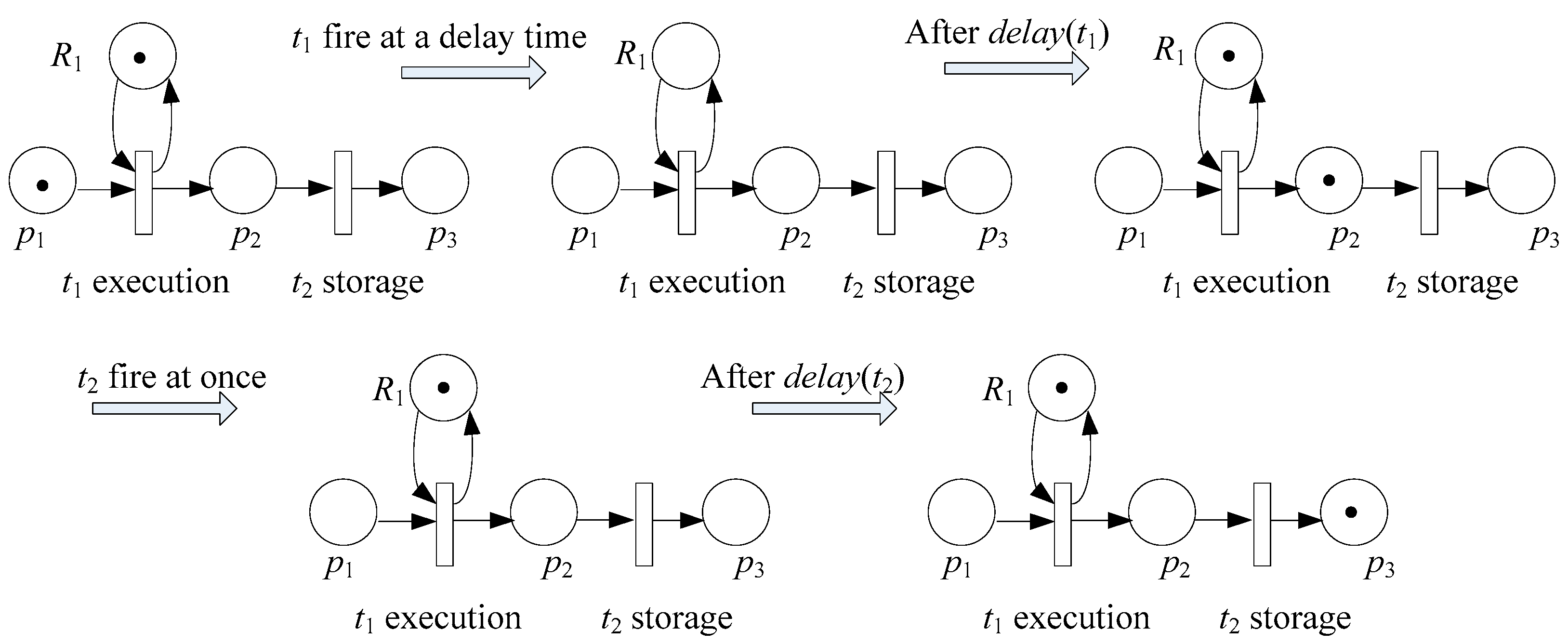
The S3PR methodology is followed to model the FJSP-IT since it is able to meet the modeling requirements of a generic FJSP [35]. Each execution is modeled with an active transition, each storage is modeled with a passive transition, each job is modeled with a sequence of operation places and each machine is modeled with a resource place. Initially, the first operation place of each job and each resource place have one token and the other places have no token. Thus, the initial marking of a PN meets the assumptions that all machines are available and that all jobs are released at a given start time. Expanding the PN structure in [41], the structure of a PN with an execution and its successive storage is shown in Figure 3.
In the above PN, p1, p2 and p3 are operation places, R1 is a resource place, t1 denotes an execution with machine R1, t2 denotes the successive storage of t1, t1 is active and t2 is passive. At the initial time, M(p1) = 1, M(r) = 1, M(p2) = 0 and M(p3) = 0. Transition t1 is enabled and will fire at a delay time, and then, M(p1) = 0 and M(R1) = 0. After tm(t1), t1 will release, M(r) = 1, M(p2) = 1, t2 will fire at once, and M(p2) = 0. After tm(t2), t2 is releasable and M(p3) = 1; however, t2 will not actually release until its successive active transition fires.
According to the assumptions that all jobs are independent of each other and the order of operations for each job is predefined, each job is modeled with a subnet. According to the assumption that each machine can execute only one operation at a time, all job subnets are connected by shared resource places and incorporated into a full PN. The weights of all arcs and the bounds of all places are 1 since each job state or each machine is modeled with a place. Thus, the indirect energy of the FJSP-IT is modeled with PNs as well as complex sequence and resource constraints.
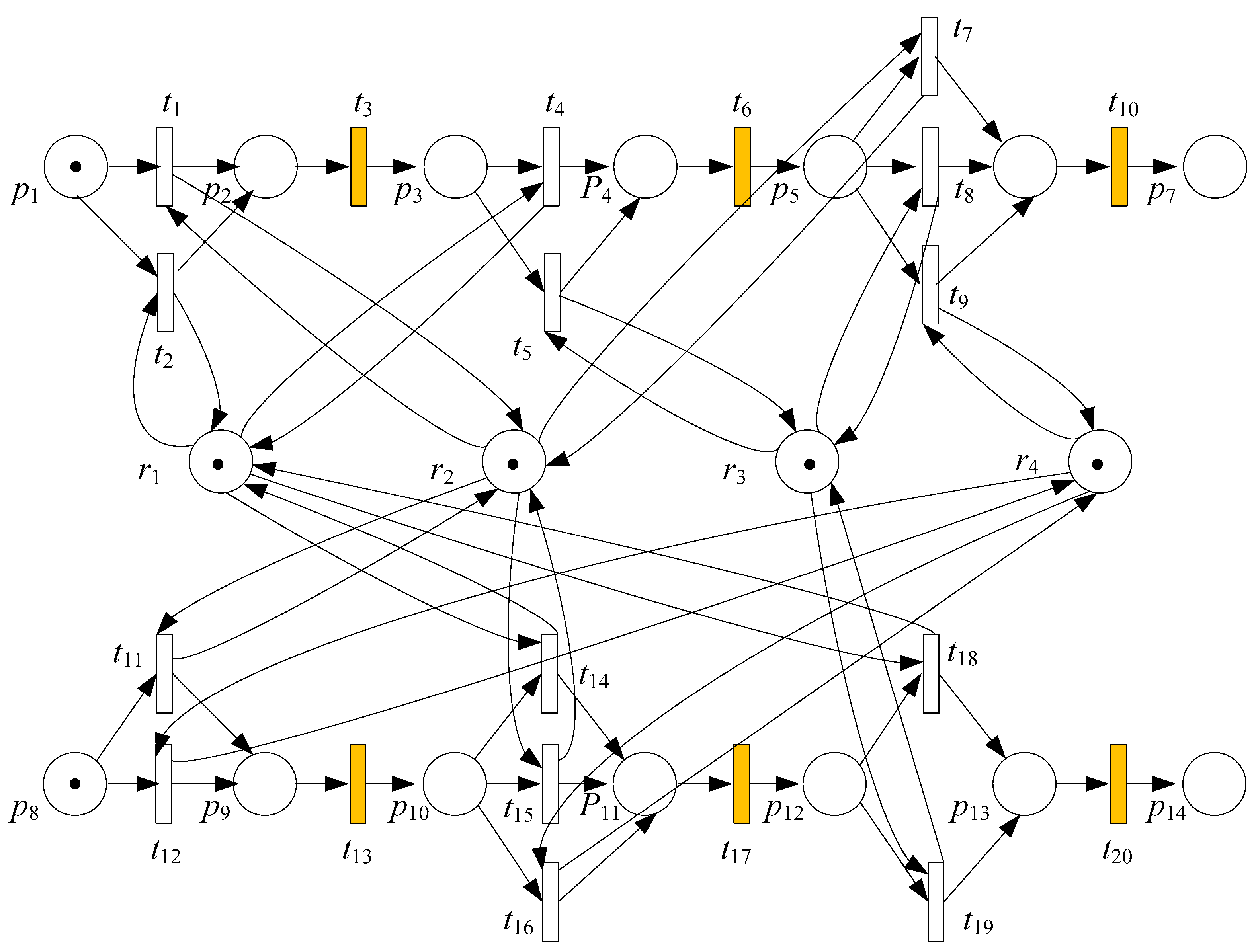
Taking 2 jobs J = {J1, J2}, 3 operations Oj =< Oj,1, Oj,2, Oj,3 > (j = 1,2) and 4 machines R = {R1, R2, R3, R4} as examples, each job has 3 operations and 3 storages. The available machines and power and time consumption of operations and storages are shown in Table 1.
In Table 1, pwr and tm on line 2 denote power and time consumption, respectively; their units are kilowatt (kW) and hour, respectively, and the slashes below line 3 mean that the operation on column 2 cannot be executed by the corresponding machine. Figure 4 illustrates the PN model for the example in Table 1.
In Figure 4, places r1, r2, r3 and r4 denote machines R1, R2, R3 and R4, places p1, p2, …, p7 denote the states of J1, transitions t1, t2, …, t10 denote the available executions and storages of J1 and the branching transitions represent the possible executions for one operation, e.g., t1 and t2 denote the 2 executions X1,1,2 and X1,1,1 for O1,1. The above places and transitions and the arcs between them constitute the subnet of J1. Similarly, places r1, r2, r3 and r4, places p8, p9, …, p14, transitions t11, t12, …, t20 and the arcs between them constitute the subnet of J2. The two subnets are incorporated into the full PN through the shared resource places r1, r2, r3 and r4. The power and time consumption is represented as the pwr and tm property of a transition, respectively, and execution and storage are distinguished by the act property of a transition. Passive transitions (denoting storages) are filled with color in the figure.
4. Proposed GAPN Approach for the FJSP-IT
4.1. Framework
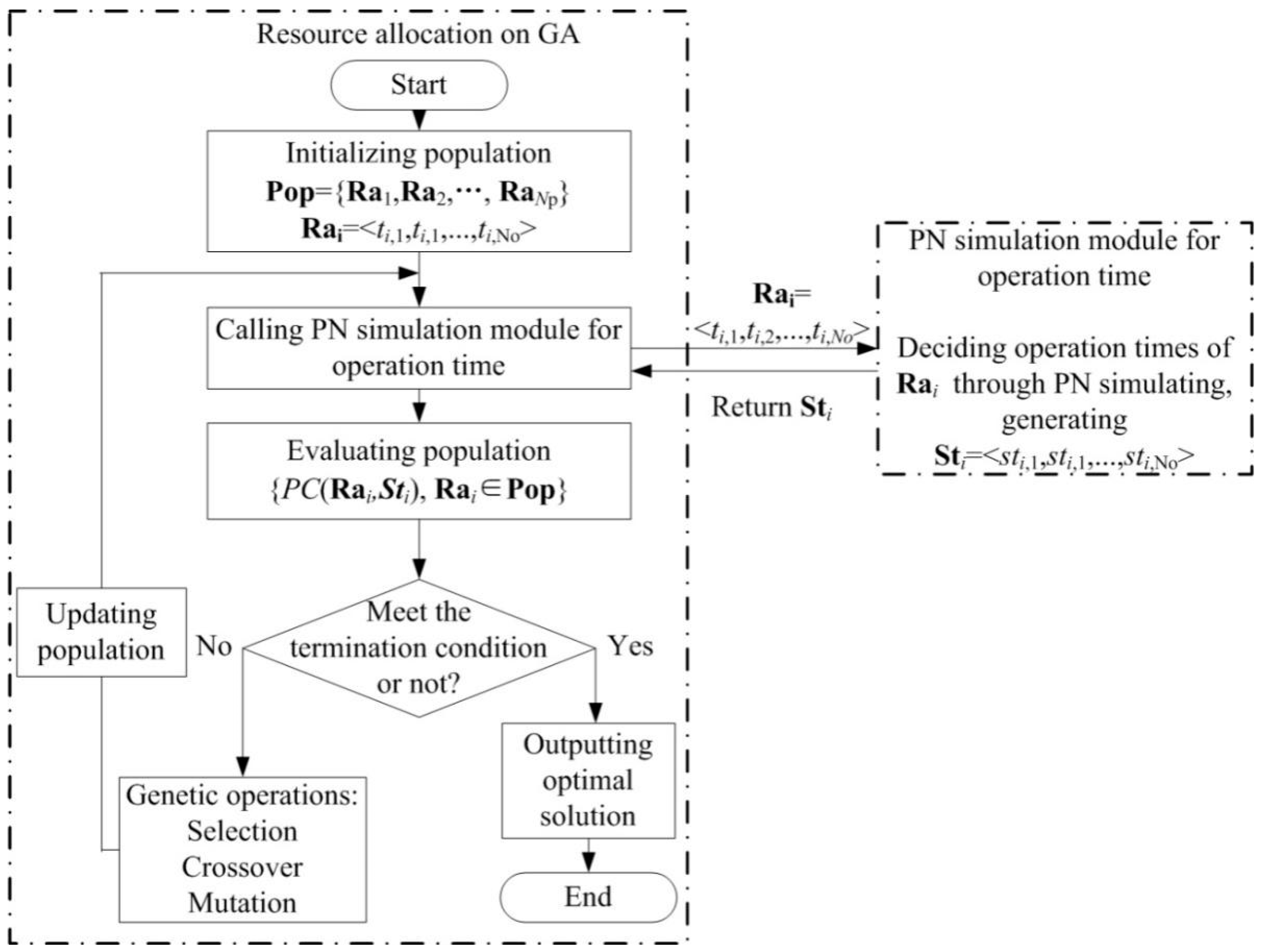
The frameworks for the GAPN approach in [39,49] decomposed FJSPs into resource allocation and objective simulation, and PN models allowed simulation with complex control policies. The proposed GAPN approach for the FJSP-IT will extend the indirect energy considerations and operation time decisions on the basis of decomposition and simulation. As mentioned in the problem definition, the decision of FJSP-IT involves determining allocate(o) and start(o), and start(o) will significantly expand the solution space. If the FJSP-IT is considered as a one-shot problem, the optimal solution will be hard to search. Additionally, operation time policy will be hard to evaluate with undetermined allocate(o). To reduce the complexity of FJSP-IT, a solution to the FJSP-IT is decomposed into resource allocation (deciding Ra) and operation time (deciding St) decisions. Resource allocation is fine-tuned using the GA, and the operation time is evaluated using PN simulation of heuristic policies. The framework of the GAPN approach for the FJSP-IT is shown in Figure 5.
In Figure 5, Pop is a group of resource allocations and denotes the population of the GA. Based on the definition and PN model of the FJSP-IT, Rai, which is one element of Pop, is a set of active transitions modeled with executions. To meet the sequence constraints on operations, let Rai = <ti,1, ti,1, …, ti,h>, where h is the size of operation set O and elements are preordered by the operation time. For example, Rai = <t1, t4, t8, t11, t14, t18> and Sti = <0, 10, 23, 34, 48.5, 59.7> is a valid solution to the example illustrated in Figure 4. Rai is encoded as a chromosome of the GA, Sti is solved by calling the PN simulation module for the operation time, which inputs Rai and returns Sti, PC(Rai,Sti) is the fitness of Rai and the resource allocation of a FJSP-IT is fine-tuned through selection, crossover and mutation.
The PN simulation module for the operation time is first presented in the next subsection, and then, the initializing population, selection, crossover and mutation are designed.
4.2. Operation Time Policies and PN Simulation
4.2.1. Operation Time Policies
The operation time policy is the base of PN simulation. We summarize the existing policies into three types, i.e., passive delay, off-peak first and highest density first, and we point out their limitations for the FJSP-IT. Any single policy is hard to adapt to the vague cost components of the scheduling problem and, hence, we present five heuristic policies, including the compatible policies of passive delay, off-peak first and highest density first.
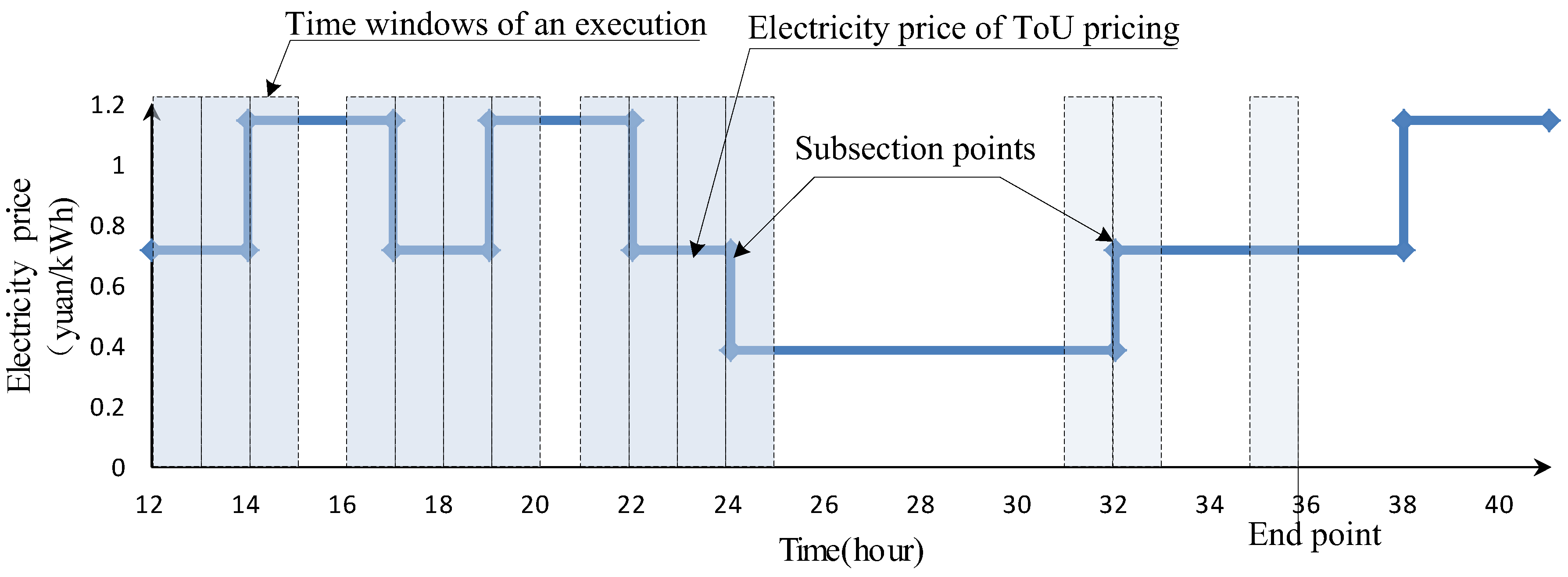
The heuristic policies are based on the daily sectioned function of ToU pricing. The daily characteristic of ToU pricing determines that the economical operation time must be within the 24 hours after the operation is enabled, and the sectioned characteristic of ToU pricing determines that the economical operation time must be located at one of the subsection points. Moreover, only an operation time delay passing over a price period can change the electricity cost; otherwise, the delay will mostly increase the time cost. Therefore, for an execution Xj,k,i (an operation to be executed), its candidate operation time can be derived by moving the time window with width tm(Xj,k,i) and matching the subsection points. For example, an execution with a time consumption of 1 h is enabled at 12:00 under ToU pricing in Guangdong, China (shown in Table 2), and its candidate set of start times is shown in Figure 6.
In Figure 6, the horizontal axis denotes the time in increments from the enabled time 12:00, the vertical axis denotes the electricity price, the line denotes the electricity price of ToU pricing and the rectangles filled with color denote the time window of execution. The subsection points (12, 14, 17, 19, 22, 24, 32, 36) can be found on the line. The first candidate operation time is just the enabled time 12:00. Then, the time window is moved right to the end point (the value 36 means 12:00 after 24 h). When the left or right end of the time window overlaps with a subsection point, the time of the left end is appended to the candidate operation time set. The candidate set of operation times in this example is (12, 13, 14, 16, 17, 18, 19, 21, 22, 23, 24, 31, 32, 35).
Due to the complex sequence constraints and shared resource constraints, the overall production cost incurred by an operation time delay is hard to evaluate. We use the predicable parts of adjacent storages and operations to evaluate operation times. The cost evaluation of an individual operation time is shown in Equations (11) and (12):
where start0(Oj,k) is the enabled time of Oj,k, EC(Si,j−1) denotes the electricity cost of the previous storage, denotes the electricity cost of evaluating the operation, Δd denotes the operation time delay from the enabled time and means the production cost related to the delay, including the electricity cost of the previous storage, the electricity cost of evaluating the operation and the time cost of the delay.
Based on the candidate set and cost evaluation of operation times, an exhausting subsection policy is first presented. Then, compatible policies, including the passive delay policy, the off-peak policy and the highest density first policy, are presented by reducing the candidate set of operation times. Finally, mixed policies are presented by mixing two basic policies.
Exhausting subsection (EXS) policy: We evaluate each operation time in the candidate set and then choose the element with the minimal cost as the economical operation time.
Passive delay (PSV) policy: The candidate set includes only the enabled time of operation.
Off-peak first (OPF) policy: The elements in the candidate set should meet the conditions that an operation starts at the start point of the off-peak price period or ends at the end point of the off-peak price period.
Passive delay with the highest density first (PDF) policy: This policy tries to approximately implement the highest density first policy for the FJSP-IT, the operation times of the top n operations with the highest power density are decided using the off-peak first policy, and the others are decided using the passive delay policy.
Exhausting subsection with the highest density first (EDF) policy: The operation times of the top n operations with the highest power density are decided using the off-peak first policy and the others are decided using the exhausting subsection policy.
As mentioned above, the PSV policy is effective for time cost-intensive shop scheduling and the OPF policy is effective for energy-intensive shop scheduling. The EXS policy, PDF policy and EDF policy are designed for shop scheduling with vague cost components. The EXS policy is a novel policy inspired by stepwise optimization. It is the most flexible for choosing the operation time and is expected to have a wide space of coverage. While solving the FJSP-IT, the five heuristic policies are evaluated using the production cost, and the optimal policy is adopted.
4.2.2. PN Simulation Algorithm for Operation Time Decisions
A PN simulation algorithm is presented on the basis of the above heuristic policies and the PN model for the FJSP-IT. The input of the algorithm is an active transition sequence, namely, Rai = <ti,1, ti,2, …, ti,No>, which models with a resource allocation in the PN for the FJSP-IT, and the output of the algorithm is an operation time sequence Sti. The notations defined above are available in the algorithm and other parameters are defined as follows:
| tmr | The running time of the PN |
| Tw | The sequence of waiting transitions |
| Te | The sequence of enabled transitions |
| Tr | The sequence of running transitions |
| Fr | The map from transitions to fire times |
| Rr | The map from transition to release times |
The transitions in Rai go through four states, i.e., waiting, enabled, running and released, and they move among three sequences, i.e., Tw, Te and Tr, one-by-one and step-by-step. Removing an element from Tr means releasing a transition. Fr and Rr are used to record the fire and release times of a transition. Fr is assigned to Sti and is finally returned. Given an operation time policy, the procedure of the PN simulation algorithm (Algorithm 1) is described as follows:
| Algorithm 1 The procedure of the PN simulation algorithm. |
| initialize, set tmr = 0, M = M0, Tw = Rai, Te = ∅, Tr = ∅, Fr = ∅ and Rr = ∅; |
| while Tw is not empty or Tr is not empty do |
| for each transition t in TW do |
| if t is enabled then |
| move t from Tw to Te; |
| pre-evaluate PC(start(t)) using Equation (11); |
| Fr[t] = argmin(PC(start(t))); |
| end if; |
| end for; |
| if Te is not empty then |
| select the transition t with the earliest fire time from Te; |
| move t from Te to Tr; |
| Rr[t] = Fr[t] + tm(t); |
| M(p) = M(p) − w(p, t); |
| end if; |
| if Tr is not empty then |
| select the transition t with the earliest release time from Tr; |
| tmr = Rr[t]; |
| Remove t from Tr; |
| M(p)= M(p) + w(t, p); |
| end if; |
| end while; |
| Sti = Fr, return Sti; |
The order of transitions in sequences Tw represents the priority order of fires, which is used to solve the resource conflicts among transitions with the same fire time.
The time complexity of the algorithm can be evaluated by three basic operations: (1) pre-evaluating the fire time of transitions, (2) selecting the transition with the earliest fire/release time, and (3) updating M.
The scale of the FJSP-IT is characterized by the number of resources (m), the number of jobs (n), the number of operations (h) and the number of price periods under ToU pricing (l). Let Nt denote the number of transitions and Np denote the number of places. If an FJSP-IT has the most flexibility, each operation can be executed by any resource; thus, Nt = h × m, Np = h + n + m. If the exhausting subsection policy (the most complex operation time policies) is used, the basic operation (1) is the combination between the transition and the price period, and its time complexity is O(Nt × l), O(h × m × l). For the basic operation (2), both the size of Te and the size of Tr are no more than min{m, n} and, hence, its time complexity is O(Nt × min{m, n}), O(h × m × min{m, n}). For the basic operation (3), M(p) = M(p) − w(p, t) and M(p) = M(p) + w(t, p) are matrix summations and loop Nt times; hence, their time complexity is O(Nt × Np), O(h × m × (h + n + m)). The whole time complexity is O(h × m × (h + n + m + l+ min{m, n})). The basic operations (2) and (3) are the necessary computation steps for a generic FJSP simulation of PNs, and parameter l is usually a small number (equal to 6 in Table 2). Therefore, using the exhausting subsection policy will not significantly increase the time complexity of PN simulation.
4.3. The Main Operations of the GA
4.3.1. Initializing the Population
A valid chromosome Rai has to meet two conditions: (1) there is only one transition for each operation; (2) the order of transitions is in accord with the predetermined sequence of operations. Therefore, the length of chromosomes is equal to the size of operation set O.
The initial population needs to guarantee the diversity of operation sequences and resource allocations. The former is guaranteed as follows: (1) a random permutation of the integers from 1 to the size of O is generated; (2) the random permutation is divided into n segments, and the length of the jth segment is hj; (3) each segment is independently ordered, and the jth ordered segment represents the operation position set of Jj. We use the example illustrated in Figure 4 to explain. If the random permutation is I = <6, 3, 5, 1, 4, 2>, then I is divided into I1 = <6, 3, 5> and I2 = <1, 4, 2> since the operation number of each job is 3. After segment ordering, I1 = <3, 5, 6>, I2 = <1, 2, 4>, and I = <3, 5, 6, 1, 2, 4>. I is the position number of O = <O1,1, O1,2, O1,3, O2,1, O2,2, O2,3>.
The latter is the random resource allocation to each operation. In the example illustrated in Figure 4, X1,3 ={ X1,3,2, X1,3,3, X1,3,4} denotes the execution set of O1,3 modeled with transitions {t7, t8, t9} in the PN, and one of them is randomly selected as an element of Rai. Assuming that the operation sequence has been determined as I = <3, 5, 6, 1, 2, 4>, t1, t5, t8, t11, t15 and t19 are selected for O1,1, O1,2, O1,3, O2,1, O2,2 and O2,3, respectively. Then, the corresponding chromosome is Rai = <t11, t15, t1, t19, t5, t8>.
4.3.2. Selection
The selection process operates on two levels. First, a certain number of chromosomes with the best fitness (lowest production cost) are selected from the parent population to fill the child population. Then, the roulette wheel strategy is performed on the remaining parent individuals, in which an individual chromosome is selected to fill the child population with a probability proportional to its fitness.
4.3.3. Crossover
The crossover randomly chooses two different individual chromosomes from the parent population and then creates two different child chromosomes by crossing the parents over. Different from a generic GA, the child chromosomes created by the simple crossover will not meet the constraints of the operation sequence and resource share. To maintain the validation of the child chromosomes, the genes of the parents are reordered by the job and the operation before crossover. The reordered parents can support simple crossover since they have a consistent match between the gene position and the operation position.
Classical one-point crossover is adopted and works as follows: (1) two parents are randomly selected from the parent population; (2) the genes of the two parents are reordered by the job and the operation; (3) one cross point (from 1 to the length of a chromosome) is randomly created; (4) two child chromosomes are created by crossing the parents over at the cross point; (5) the order of genes in the two child chromosomes are restored to the original.
4.3.4. Mutation
Mutation is used to maintain genetic diversity in the population. Each individual chromosome subject to the crossover has the possibility of being subject to the mutation process. In this algorithm, two mutation strategies are adopted: gene substance mutation and gene position mutation. The former randomly selects one gene and replaces it with another transition modeled with the same operation, while the latter randomly selects one gene and moves it to another valid position. In the chromosome Rai = <t11, t15, t1, t19, t5, t8> in the example illustrated in Figure 4, t15 has the possibility to change to t14 or t16 when using gene position mutation, and it has the possibility to move from position 2 to 4. Gene substance mutation is a type of traditional mutation, and gene position mutation is a novel mutation that can change the priority order of operations.
The mutation works as follows: (1) each individual in the parent population is selected based on a predefined mutation probability; (2) a predefined number of genes is randomly selected from the selected individual, and gene substance mutation and gene position mutation are performed.
5. Experiments and Results
5.1. Design of the Experiments
This subsection discusses the data set used for experiments, the comparison benchmark for the proposed approach, the GA parameters and the test environment.
5.1.1. Data Generation
Compared with a generic FJSP, the FJSP-IT extends concepts such as storage and power, and existing data sets for generic FJSPs need to be extended to adapt to the experiments in this paper. We generated a new data set based on the banburying shop of a rubber tire plant, one of our cooperative enterprises in Guangdong, China. The scheduling requirements of this enterprise motivated this study. Banburying converts raw rubber and other auxiliary ingredients into a strong and elastic mixture by stirring and rubbing in an internal mixer. One job needs to go through two or three banburying operations before being delivered to the next job shop. One operation can be executed by several internal mixers, and one job needs to be subject to a slow chemical reaction in a cool storage area after each banburying operation. Banburying is a typical power-intensive operation, and storage areas need HVAC to maintain the environment. Hence, banburying production conforms to the definition of the FJSP-IT. The cooperative enterprise produces hundreds of rubber tire types, and the studied shop processes hundreds of job types using 15 internal mixers with different energy efficiencies and capacities. Banburying is not a production bottleneck and hence there are chances that it can delay the operation time.
We regard banburying a batch of material as a job and banburying as an operation, and a possible internal mixer assignment to an operation as an execution. The power and time consumption of an execution was set based on the process parameters, the power consumption of a storage was set based on the power share of the HVAC system and the storage time was set based on the process parameters. We chose 60 job records from past production logs to build the experimental data set. The power and time consumption of an execution (or a storage) is distributed as shown in Table 3.
To characterize the scale of the job set and resource set, we built four test cases by randomly selecting jobs and resources. They are marked by m × n, which denotes m machines processing n jobs. The four test cases were marked by 4 × 6, 8 × 15, 12 × 25 and 15 × 40. The operation number of jobs was two or three. Notably, two jobs in case 4 × 6 are shown in Table 1 and the remaining four jobs are shown in Table 4. Case 4 × 6 is used as an example for detailed analysis.
When evaluating the production cost, a time cost of K = 200 was set based on the idle labor cost caused by an operation time delay, and ToU pricing adopted the electricity price in Table 2.
5.1.2. GA Parameter Setting
The following empirical values were adopted for the GA parameters [13]:
Population size: max (2 × n × h,100), h denotes the number of operations;
Selection probability: 0.75;
Mutation probability: 0.15;
Crossover probability: 0.50;
The retained number of chromosomes with the best fitness: 3;
The maximum number of iterating generations: max(n × h, 300);
The terminating condition of iteration: the iterating generations reach the maximum number, or the best fitness remains unchanged for 30 generations.
5.1.3. Benchmark Heuristics
Experiments were designed to verify the convergence of the proposed GAPN approach, the effectiveness of indirect energy considerations and the effectiveness of operation time policies.
To verify the convergence of the proposed GAPN approach, the GA with only gene substance mutation was selected as a benchmark for that with additional gene position mutation, and the convergence speed and quality were compared with each other.
To verify the effectiveness of the operation time policies, the off-peak first policy and passive delay policy, the two policies in real production and the literature [3,5,20,21], were used as the benchmark for the presented policies: the exhausting subsection policy, the exhausting subsection with the highest density first policy and the passive delay with the highest density first policy. The characteristics of the solution, such as the cost component, resource allocation and power distribution, were calculated and compared among the operation time policies.
To verify the effectiveness of considering indirect energy, the objective (see Equations (1)–(9)) and the cost evaluation of the operation time (see Equations (11) and (12)) excluding indirect energy were used as benchmarks. The characteristics of the solution, such as the cost component, resource allocation and power distribution, were calculated and compared between the objective including indirect energy and that excluding indirect energy.
5.1.4. Approach Implementation, Configuration and Performance
The proposed approach was implemented in the MATLAB R2018a environment. The experiments were run on a cloud server with a 4-core CPU @ 2.50 GHz, 8 GB RAM and Windows server 2012 R2 operating system.
Based on the benchmark heuristics above, the experiments were characterized by case, GA mutation policy, operation time policy and objective considerations. The approach implementation allowed characteristic configuration. For the GA mutation policy, two configurations, single mutation and double mutation, could be set. The former adopted only gene substance mutation, while the latter adopted both gene substance mutation and gene position mutation. For objective considerations, two configurations, including indirect energy and excluding indirect energy, could be set. The former evaluated the electricity cost using Equation (2) and evaluated the operation time cost using Equation (11), while the latter evaluated the electricity cost excluding EC(S) from Equation (2) and evaluated the operation time cost excluding EC(Si,j − 1) from Equation (11). Hence, there were four cases, two mutation policies, five operation time policies and two objective considerations in the implementation of the approach. To simplify the description, the abbreviations are defined in Table 5.
Theoretically, 80 (4 × 2 × 5 × 2) configurations can be set. A configuration is marked by the abbreviated characteristics and the symbol &, e.g., C4 × 6&DBM&EXS&IIE represents the configuration with case 4 × 6, the DBM mutation policy, the EXS operation time policy and the IIE objective consideration. The mutation policy and objective consideration can be omitted, and DBM and IIE are default values, e.g., C4 × 6&EXS has the same configuration as C4 × 6&DBM&EXS&IIE.
To evaluate the performance of the configuration, the iteration number of termination is used to evaluate the convergence speed of the configuration, and the production cost is used to evaluate the solution quality of the configuration. To simplify the description, PC, DEC, IEC and TC are the abbreviations of the production cost, direct energy cost, indirect energy cost and time cost, respectively. For a group of replicated configuration experiments, the solution with the minimal PC is defined as the optimal solution. For a group of comparative experiments, the configuration obtaining the minimal PC is defined as the optimal configuration. To compare the difference between two configurations, the relative percentage deviation (rpd) is defined as rpd = (C1 − C2)/C1*100%, where C1 is the benchmark configuration and C2 is the comparative configuration.
Three groups of comparative experiments were performed on the following configuration combinations.
Convergence experiments: {SGM, DBM} combining all cases, EXS and IIE.
Operation time policy experiments: {EXS, PSV, OPF, EDF, PDF} combining all cases, DBM and IIE.
Objective consideration experiments:{IIE, EIE} combining all cases and their optimal operation time policy in the previous operation time policy experiments.
To mitigate randomness, each configuration was subjected to 20 replications. The PC, DEC, IEC and TC of each experiment were recorded, and the Gantt chart and power chart of each experiment were plotted.
5.2. Analysis of the Results
The minimal PC and mean PC obtained by replicated configuration experiments are shown in Table 6 and Table 7, respectively. In header cells, “Mut.” is the abbreviation of the mutation policy, “O.T.” is the abbreviation of the operation time policy and “Obj.” is the abbreviation of the objective consideration. The slashes in data cells denote that the corresponding configurations were not performed. The performed configurations covered convergence experiments, operation time policy experiments and objective consideration experiments.
5.2.1. Convergence of the GAPN Approach
For each experiment, the minimal iteration means the minimal number of iterating generation to reach the optimal solution. For each configuration, the minimal iteration means the minimal one of the minimal iterations of replicated configuration experiments, and the mean iteration means the mean value of the minimal iterations of replicated configuration experiments. The minimal iteration and mean iteration of the convergence experiments are shown in Table 8. The rpds between DBM and SGM are shown in Table 9, where SGM is the benchmark configuration.
From Table 8 and Table 9, we see that both the minimal iterations and the mean iterations of DBM for all cases are less than those of SGM, and the results show that the convergence speed of DBM is faster than that of SGM. We see that both the minimal PCs and the mean PCs of DBM for all cases are less than or equal to those of SGM. Especially for case 12 × 25 and case 15 × 40, which are larger scale, the rpds between DBM and SGM are significant. The results show that the additional gene position mutation can improve the convergence quality for complicated FJSP-ITs.
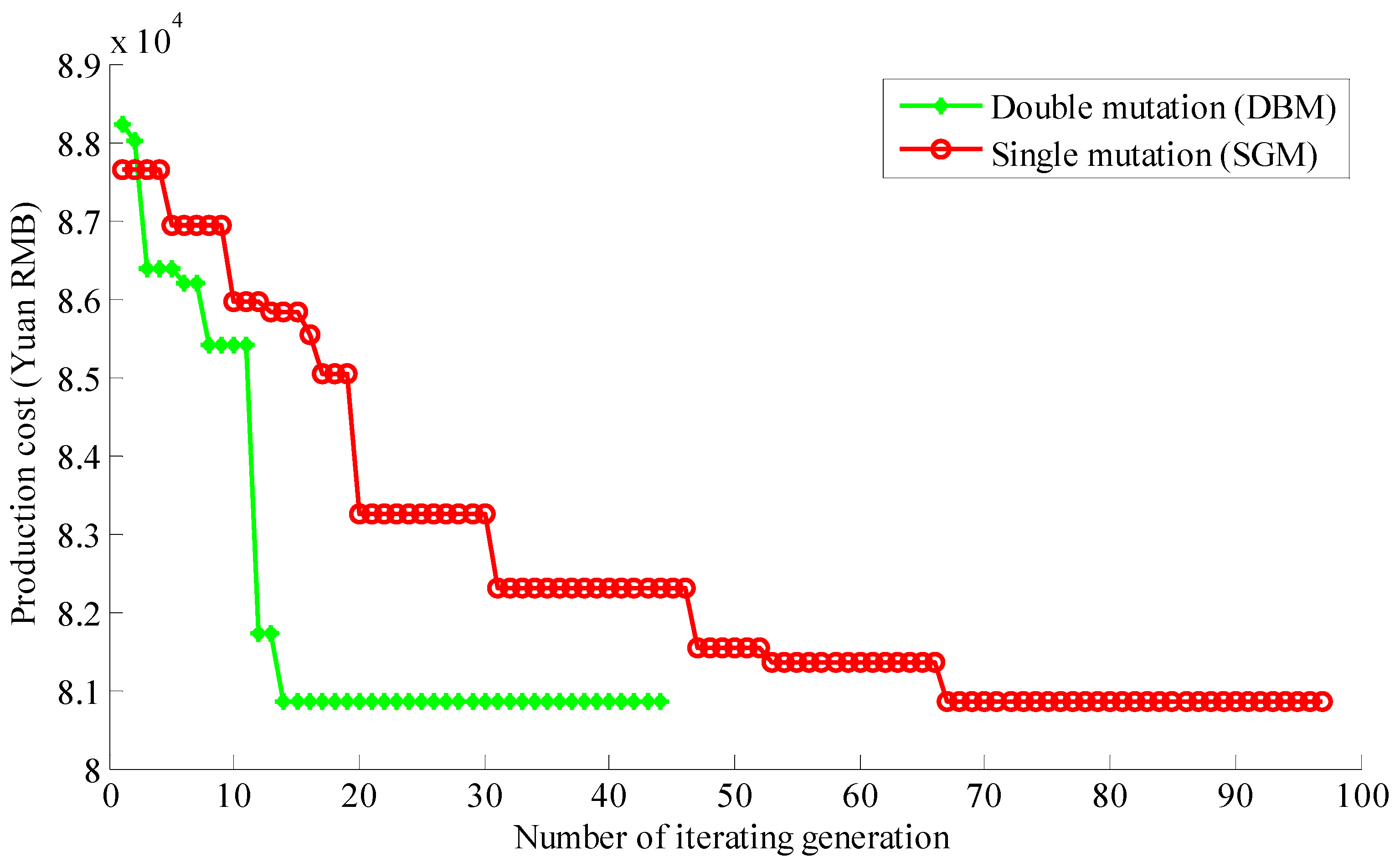
Figure 7 shows the convergence curves of the optimal solutions for configurations C4 × 6&DBM and C4 × 6&SGM. The curve with circular points denotes the configuration with DBM (double mutation) and the curve with prismatic points denotes the configuration with SGM (single mutation). The figure shows the accelerating convergence effect of gene position mutation in detail. We see that gene position mutation can help local minimal points to stand out and to improve convergence speed and quality. In larger cases, more local minimal points hide in the larger solution space; thus, gene position mutation can obtain greater improvement by enhancing population diversity.
5.2.2. Comparison among Operation Time Policies
Observing the minimal PCs and mean PCs from Table 6 and Table 7, we see that the PSV policy obtained the solutions with the worst quality for all cases. Hence, we set the PSV policy as the benchmark configuration, and the rpds of the operation time policy experiments are shown in Table 10.
From Table 10, we see that the EDF policy is the optimal policy of case 4 × 6, the EXS policy is the optimal policy of case 8 × 15, the PDF policy is the optimal policy of case 12 × 25 and the OPF policy is the optimal policy of case 15 × 40. Furthermore, the consistent judgments based on the mean PC and minimal PC show that the results have little randomness. The diversity of optimal policies shows that a single operation time policy cannot adapt to the FJSP-IT with vague cost components and using multiple operation time policies helps to trade-off between the delay cost and the electricity cost.
We also see that the rpd between the optimal policy and PSV policy ranges from 5.56% (see case 8 × 15) to 23.44% (see case 15 × 40), and the significant difference shows that the active operation time delay for the FJSP-IT can significantly reduce the production cost under ToU pricing. The rpds of case 12 × 25 and case 15 × 40 are much greater than those of case 4 × 6 and case 8 × 15. This result can be explained as follows: with the increase in jobs and machines, the feasible power tends to grow, whereas K (time cost per hour) remains constant, and the electricity cost becomes the main cost component and tends to result in more significant savings by choosing the operation time under ToU pricing.
The OPF policy is the opposite of the PSV policy. We see that it is the optimal policy only for case 15 × 40, which has the maximal proportion of electricity among the five cases. The results show that the OPF policy is not optimal for most FJSP-IT cases, although it is very prevalent in real production scheduling. For case 12 × 25, the minimal PC of the PDF policy is 10.81% higher than that of the OPF policy.
PDF is a mixture of PSV and OPF, and the minimal PC of PDF is approximately 10% less than that of OPF. This result shows that a small change in the operation time policy can significantly reduce the production cost due to the complexity of the cost factors in the FJSP-IT. EXS and EDF are inspired by stepwise optimization, and they are adaptive to cases with vague cost components. Although they are not effective for job shop scheduling with a single cost component, they play an important role in the FJSP-IT with complex cost factors.
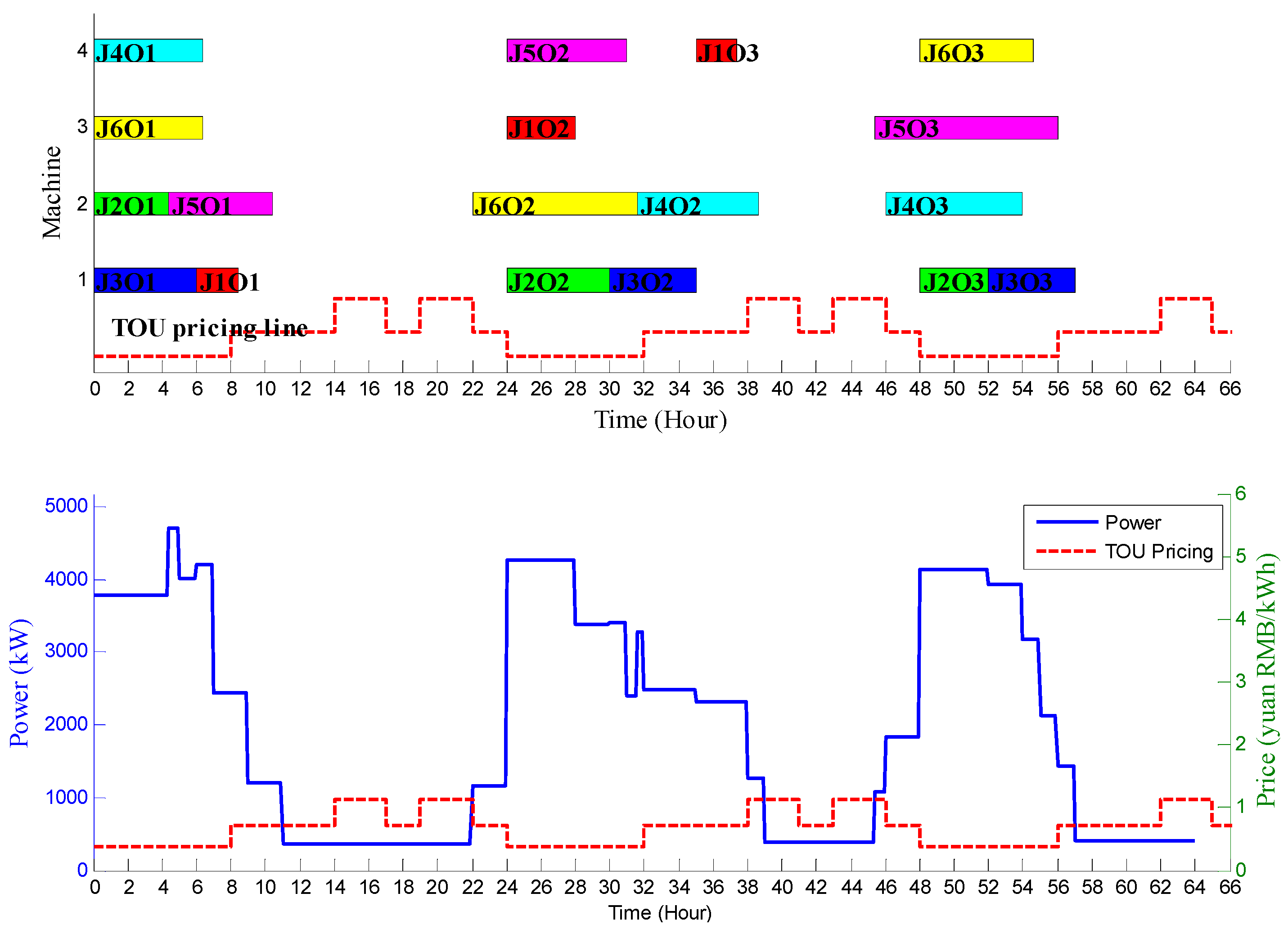
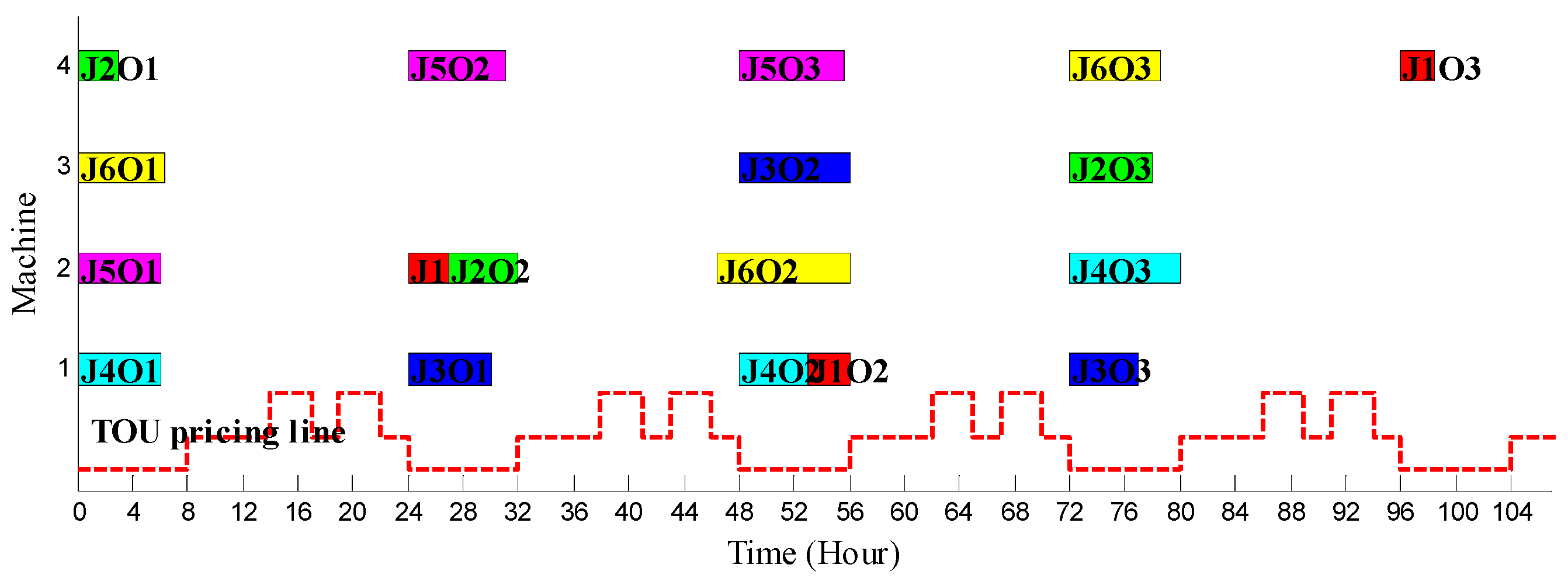
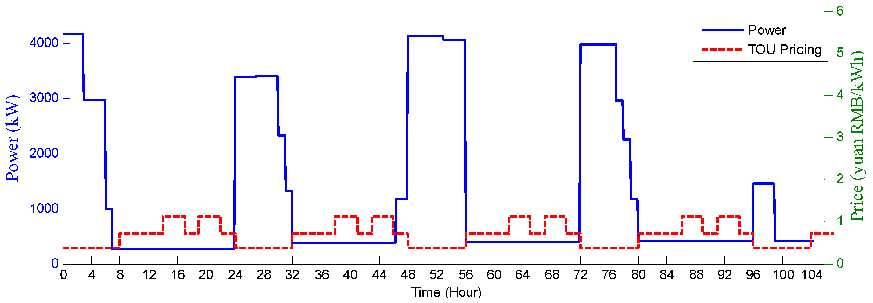
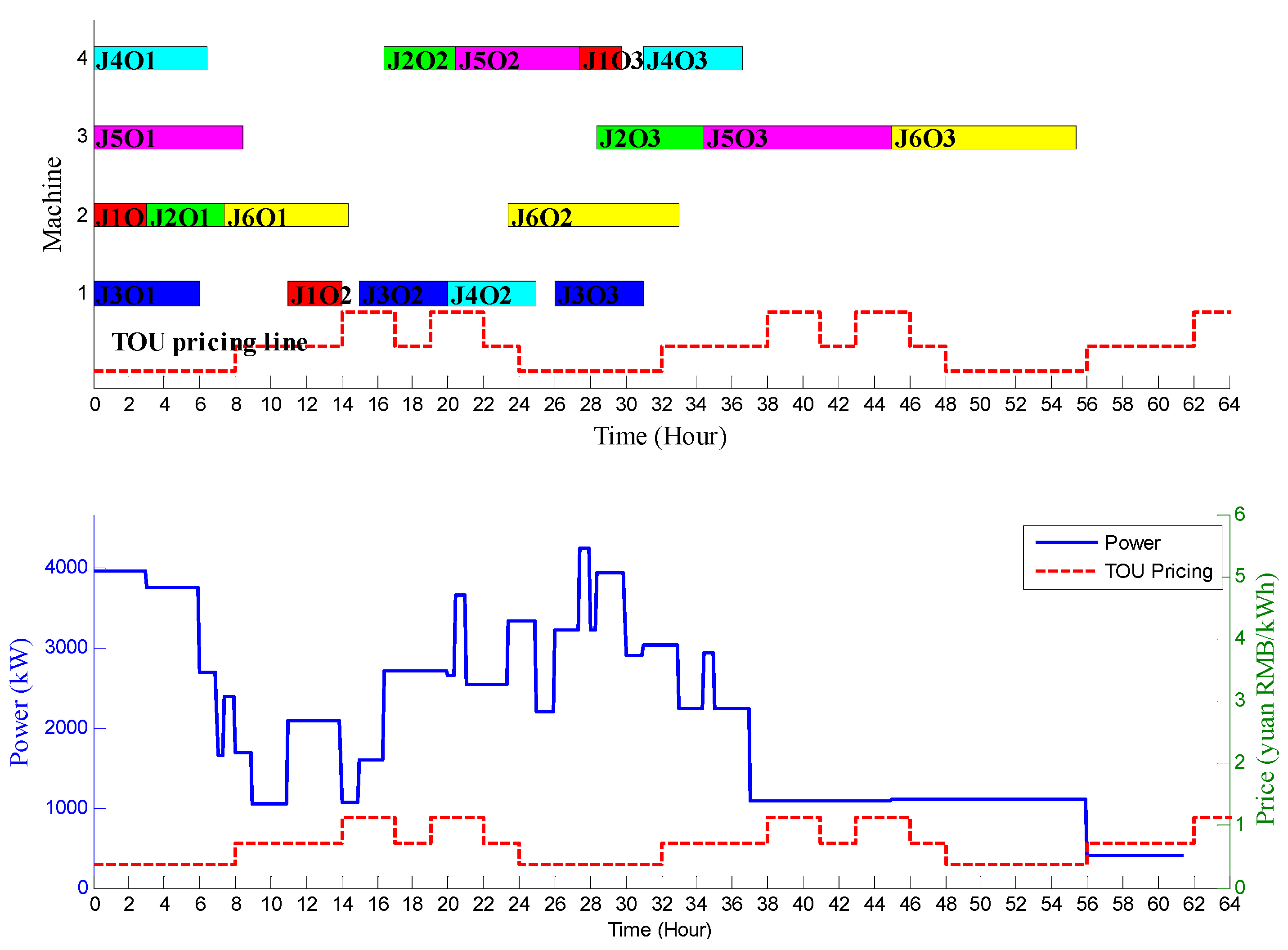
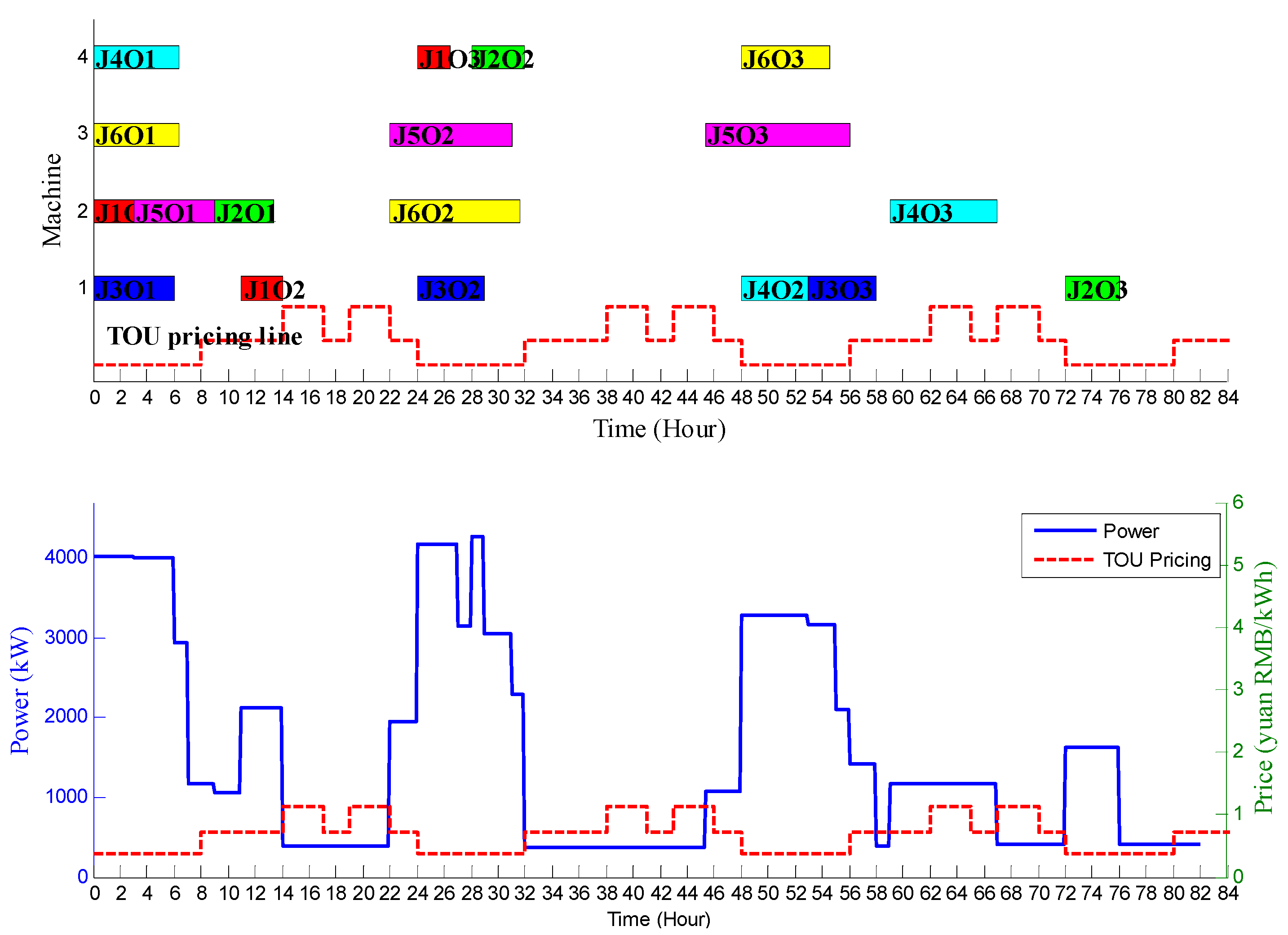
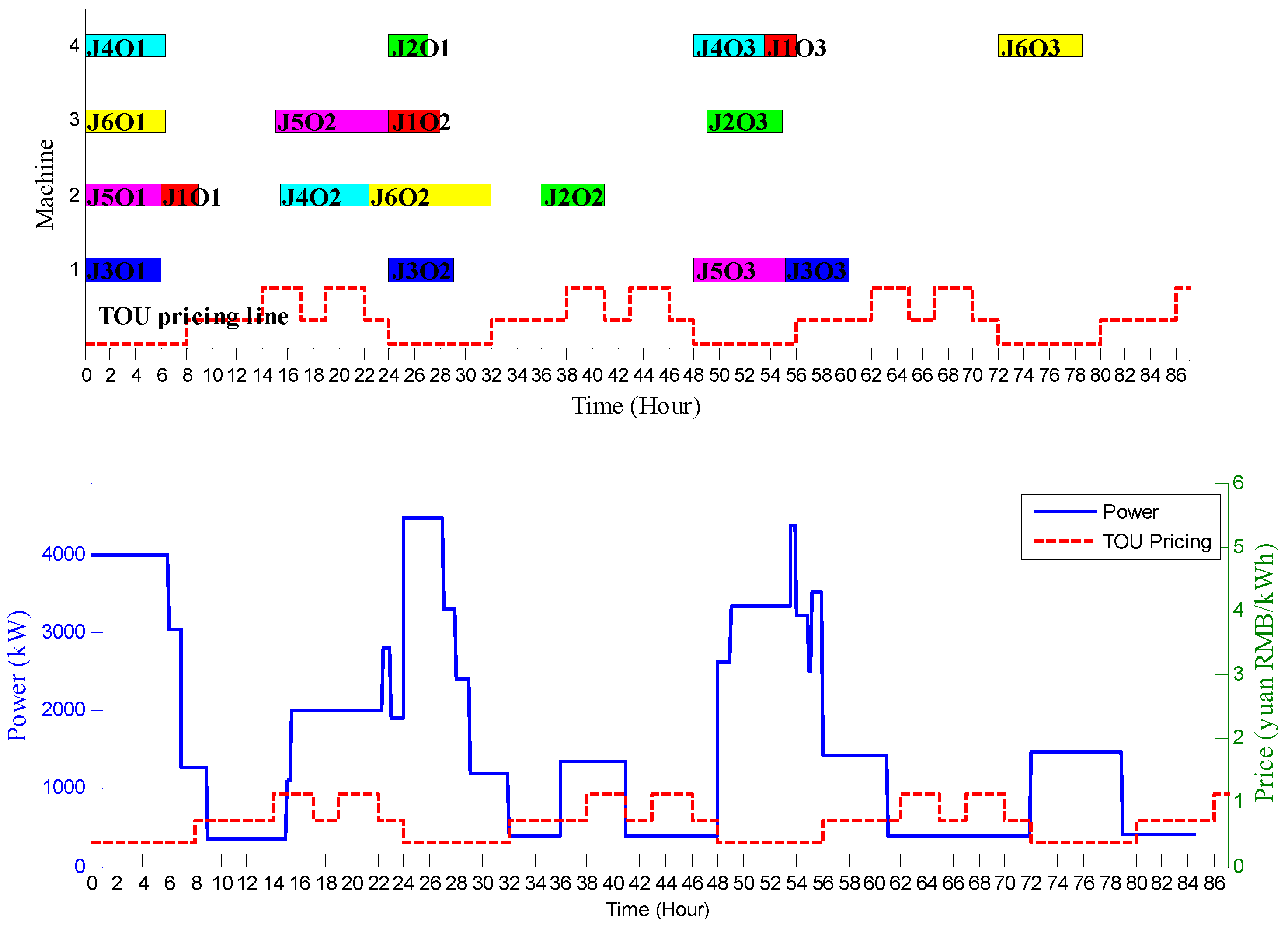
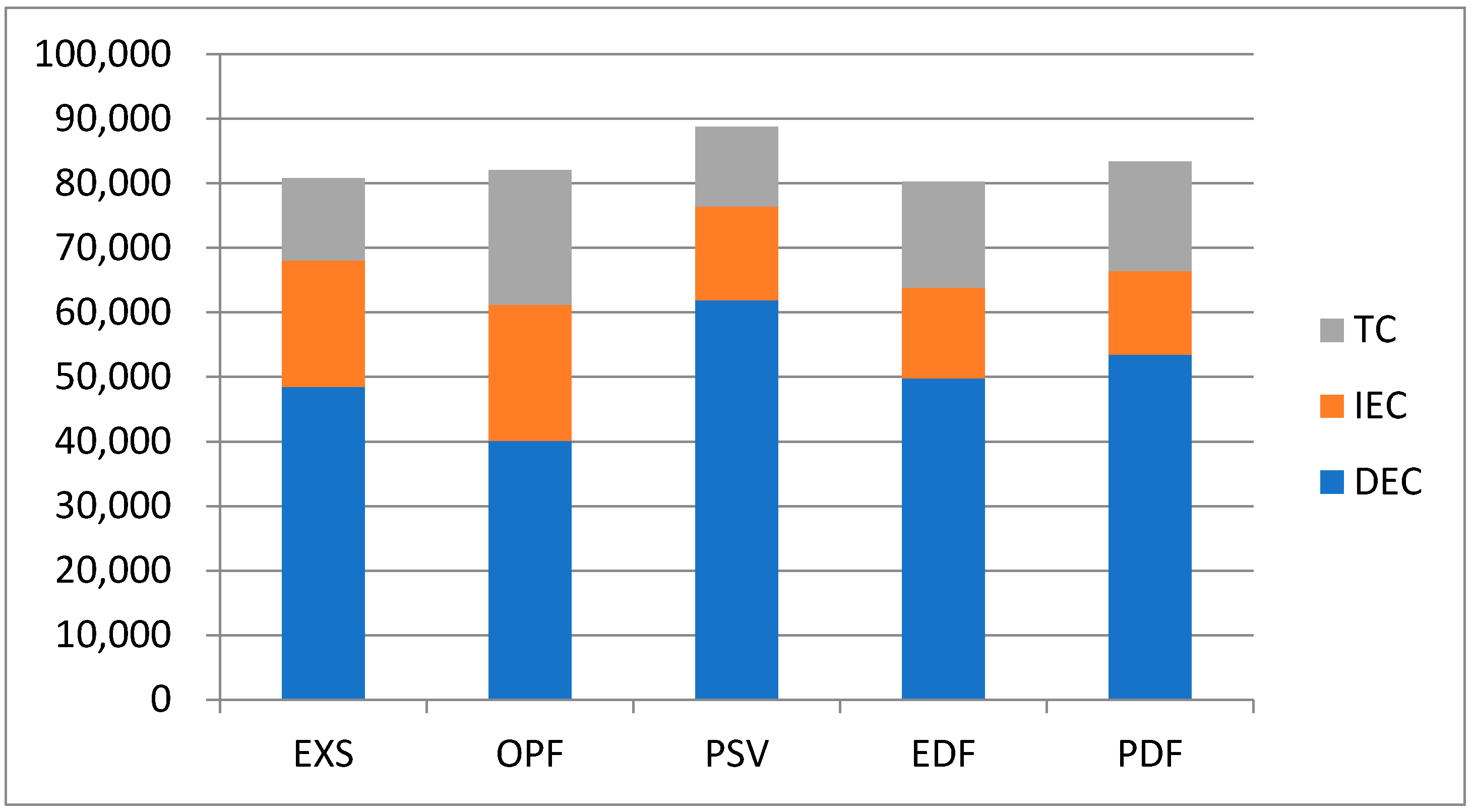
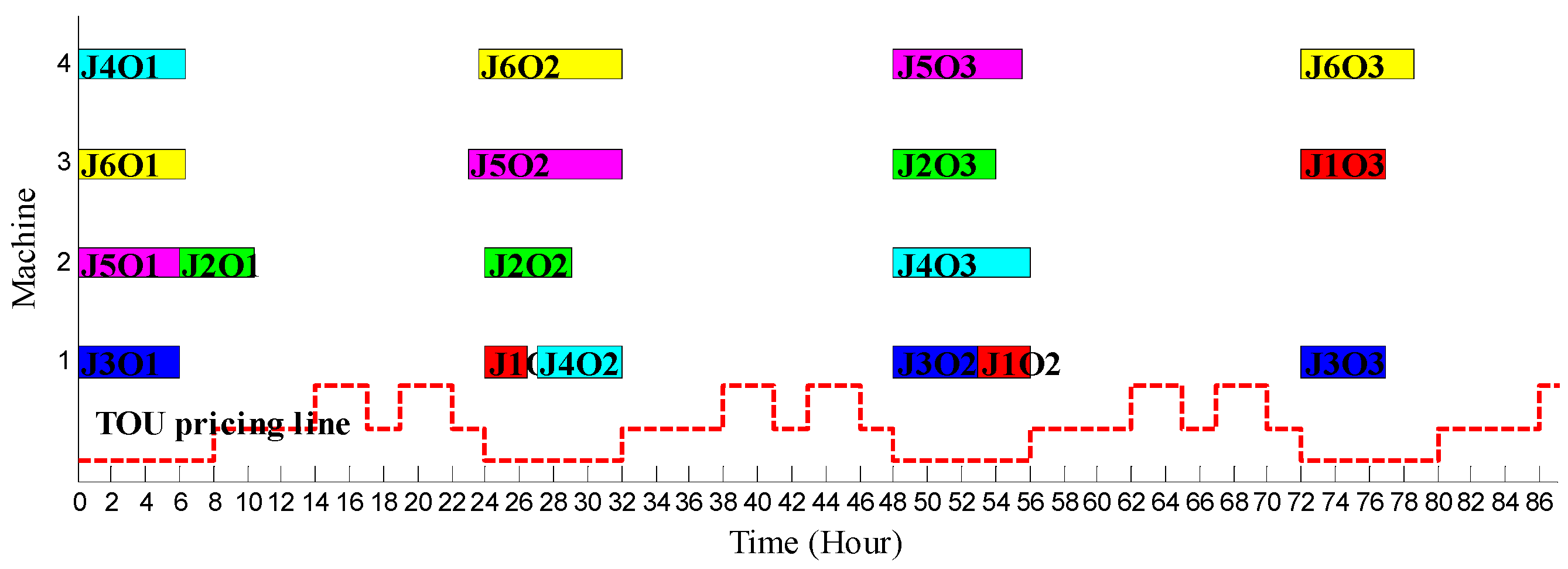
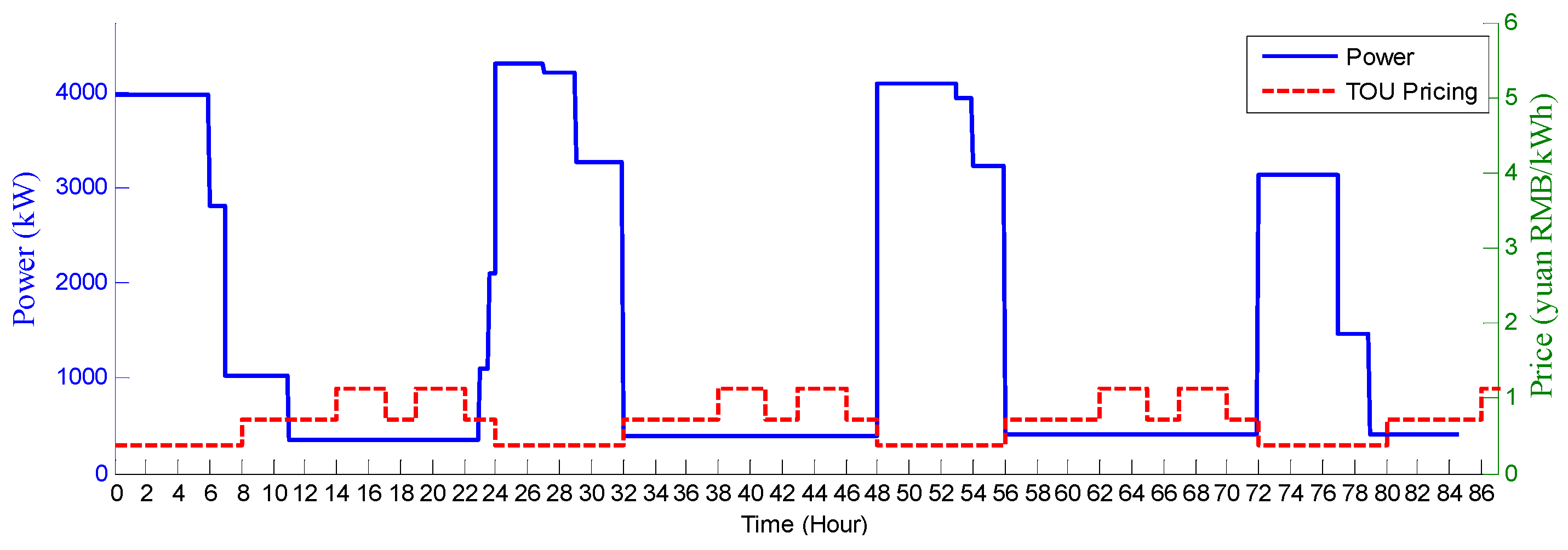
To analyze the behavioral differences between the optimal solutions to the operation time policies, we took case 4 × 6 as an example. The Gantt and power charts of the optimal solutions are shown in Figure 8, Figure 9, Figure 10, Figure 11, Figure 12, and the cost component histograms of the optimal solutions are shown in Figure 13. In the Gantt charts, each job was distinguished by different colors, and operation Oj,k was marked with text “JjOk” (e.g., J4O1 denotes O41).
Observing the power charts, we see that all power curves of the operation time policies have a change trend that is the opposite of the ToU pricing curve. Observing the Gantt charts and cost component histograms, we see the differences in optimization methods between the operation time policies. Undoubtedly, OPF obtains the maximal time cost and the minimal direct energy cost by scheduling all operations in off-peak periods, PSV obtains the minimal time cost and the maximal direct energy cost by scheduling operations without delays and PDF obtains a middle time cost and middle direct energy cost by scheduling some operations in off-peak periods and others without delays. Because of the lack of operation time options, the above three policies tend to optimize the production cost by seeking the optimal resource allocation and operation order.
Comparing the optimal policy EDF with the other policies, we see the cause of the production cost differences among the operation time policies. The operation time obtained by EDF is very similar to that obtained by EXS, and both of them obtain low production costs through a stepwise operation time choice. The small difference between them is because EDF has a slightly lower production cost than EXS by prescheduling the n operations with the highest power in off-peak periods. The time cost and indirect energy cost of EDF are much greater than those of OPF, and EDF reduces the time cost and indirect energy cost by appropriately using the mid-peak period. Compared with PSV and PDF, the direct energy cost of EDF is much lower than that of PSV and PDF, and EDF reduces the direct energy cost by appropriately delaying the operation time.
5.2.3. Comparison between the Objective Considerations including and Excluding Indirect Energy
We set EIE as the benchmark configuration, and the rpds of the objective consideration experiments are shown in Table 11.
Comparing the minimal PCs between IIE and EIE, we see that the configurations with IIE can save from 2.09–11.84% on the production cost. Comparing the mean PC of the configurations with EIE, we see that the configurations with IIE can save from 2.47–8.85% in the production cost. For the studied shop with an annual production cost of over RMB 200 million, the objective consideration including indirect energy can help to save from RMB 4.94–17.70 million, which can significantly improve the economic benefit for manufacturers with low profits.
The Gantt and power charts of the optimal solutions without considering indirect energy are shown in Figure 14. Comparing Figure 14 with Figure 11, we see that the solution to configuration C4 × 6&EDF&EIE is significantly different from that to configuration C4 × 6&EDF (default &IIE). The solution with EDF&IIE trades off between the direct energy cost and the indirect energy cost by reasonably using mid-peak and on-peak periods. The solution with EDF&EIE schedules almost all operations in the off-peak period and cannot trade-off between the direct energy cost and the indirect energy cost. Comparing Figure 14 with Figure 9, we see that the solution with EDF&IIE and the solution with OPF&EIE are similar in terms of the shape of the power distribution, and the main difference between the two solutions is resource allocation. Without the indirect energy consideration, the cost increment caused by delays is weakened and, hence, the solution with EDF degenerates to the solution with OPF. This result shows that the indirect energy consideration in objective evaluation and individual operation time evaluation is effective in trading off the cost components of the FJSP-IT.
6. Conclusions and Future Work
An FJSP-IT is investigated. Focusing on modeling indirect energy and suggesting operation time policies under ToU pricing, a GAPN approach for FJSP-IT is presented. Under this approach, indirect energy is modeled by an extended TPN model and the production cost, including the direct energy cost, indirect energy cost and time cost, is evaluated through PN simulation, resource allocation is fine-tuned through gene operations and the operation time is determined by a group of heuristic policies. To adapt to the FJSP-IT with vague cost components, a group of operation time policies, such as exhausting subsection, off-peak first, passive delay, passive delay with the highest density first and exhausting subsection with the highest density first, are presented. Convergence experiments, operation time policy experiments and objective consideration experiments are performed on a set of cases based on the banburying shop of a rubber tire plant. The results show that the proposed GAPN approach has good convergence and can obtain a satisfactory solution. For the studied cases, using multiple operation time policies makes it possible to save 10.81% on the production cost compared with using the off-peak first policy and 23.44% on the production cost compared with using the passive delay policy. Considering indirect energy makes it possible to save at least 2.09% on the production cost compared with ignoring indirect energy.
Future research may consider more elaborate problem definitions and more adaptable operation time policies. For example, a dynamic time cost model with a problem scale and makespan must be built, and auxiliary energy can be taken into objective consideration. An operation time policy with variable parameters needs to be developed to enhance adaptability to the FJSP-IT with vague cost components.
Author Contributions
Conceptualization, J.G.; methodology, J.G.; software, J.G., Q.L. and P.L.; validation, J.G., Q.L. and J.O.; formal analysis, J.G.; investigation, J.G.; resources, J.G. and P.L.; writing—original draft preparation, J.G.; writing—review and editing, J.G. and Q.L.; visualization, J.G. and Q.L.; supervision, J.G.; project administration, J.G.; funding acquisition, J.G. All authors have read and agreed to the published version of the manuscript.
Funding
This work was supported by the Natural Science Foundation of Guangdong Province (CN) (Grant No: 2018A0303130187) and the National Natural Science Foundation of China (Grant No: 62072123).
Institutional Review Board Statement
Not applicable.
Informed Consent Statement
Not applicable.
Data Availability Statement
The data presented in this study are available upon request from the corresponding author.
Conflicts of Interest
The authors declare no conflict of interest.
References
- Wang, Y.; Li, L. Time-of-use electricity pricing for industrial customers: A survey of U.S. utilities. Appl. Energy 2015, 149, 89–103. [Google Scholar] [CrossRef]
- Cochell, J.E.; Schwarz, P.M.; Taylor, T.N. Using real-time electricity data to estimate response to time-of-use and flat rates: An application to emissions. J. Regul. Econ. 2012, 422, 135–158. [Google Scholar] [CrossRef]
- Chen, B.; Zhang, X. Scheduling with time-of-use costs. Eur. J. Oper. Res. 2019, 274, 900–908. [Google Scholar] [CrossRef]
- Price, L.; Wang, X.; Yun, J. The challenge of reducing energy consumption of the Top-1000 largest industrial enterprises in China. Energy Policy 2010, 38, 6485–6498. [Google Scholar] [CrossRef]
- Zhang, S.; Zhong, J.; Yang, H.; Li, Z.; Liu, G. A study on PGEP to evolve heuristic rules for FJSSP considering the total cost of energy consumption and weighted tardiness. Comput. Appl. Math. 2019, 38, 185. [Google Scholar] [CrossRef]
- Far, M.H.; Haleh, H.; Saghaei, A. A fuzzy bi-objective flexible cell scheduling optimization model under green and energy-efficient strategy using Pareto-based algorithms: SATPSPGA, SANRGA, and NSGA-II. Int. J. Adv. Manuf. Technol. 2019, 105, 3853–3879. [Google Scholar] [CrossRef]
- Moon, J.-Y.; Park, J. Smart production scheduling with time-dependent and machine-dependent electricity cost by considering distributed energy resources and energy storage. Int. J. Prod. Res. 2014, 52, 3922–3939. [Google Scholar] [CrossRef]
- Hadera, H.; Ekström, J.; Sand, G.; Mäntysaari, J.; Harjunkoski, I.; Engell, S. Integration of production scheduling and energy-cost optimization using Mean Value Cross Decomposition. Comput. Chem. Eng. 2019, 129, 106436. [Google Scholar] [CrossRef]
- Hadera, H.; Harjunkoski, I.; Sand, G.; Grossmann, I.E.; Engell, S. Optimization of steel production scheduling with complex time-sensitive electricity cost. Comput. Chem. Eng. 2015, 76, 117–136. [Google Scholar] [CrossRef] [Green Version]
- Du, B.; Tan, T.; Guo, J.; Li, Y.; Guo, S. Energy-cost-aware resource-constrained project scheduling for complex product system with activity splitting and recombining. Expert Syst. Appl. 2021, 173, 114754. [Google Scholar] [CrossRef]
- Rahimifard, S.; Seow, Y.; Childs, T. Minimising Embodied Product Energy to support energy efficient manufacturing. CIRP Ann. 2010, 59, 25–28. [Google Scholar] [CrossRef]
- Liang, J.; Wang, Y.; Zhang, Z.-H.; Sun, Y. Energy efficient production planning and scheduling problem with processing technology selection. Comput. Ind. Eng. 2019, 132, 260–270. [Google Scholar] [CrossRef]
- May, G.; Stahl, B.; Taisch, M.; Prabhu, V. Multi-objective genetic algorithm for energy-efficient job shop scheduling. Int. J. Prod. Res. 2015, 53, 7071–7089. [Google Scholar] [CrossRef]
- Aghelinejad, M.; Ouazene, Y.; Yalaoui, A. Complexity analysis of energy-efficient single machine scheduling problems. Oper. Res. Perspect. 2019, 6, 100105. [Google Scholar] [CrossRef]
- Liang, P.; Yang, H.; Liu, G.; Guo, J. An Ant Optimization Model for Unrelated Parallel Machine Scheduling with Energy Consumption and Total Tardiness. Math. Probl. Eng. 2015, 2015, 907034. [Google Scholar] [CrossRef] [Green Version]
- Hasani, A.; Hosseini, S.M.H. A bi-objective flexible flow shop scheduling problem with machine-dependent processing stages: Trade-offbetween production costs and energy consumption. Appl. Math. Comput. 2020, 386, 125533. [Google Scholar] [CrossRef]
- Wang, J.; Liu, Y.; Ren, S.; Wang, C.; Wang, W. Evolutionary game based real-time scheduling for energy-efficient distributed and flexible job shop. J. Clean. Prod. 2021, 293, 126093. [Google Scholar] [CrossRef]
- Liu, Z.; Yan, J.; Cheng, Q.; Yang, C.; Sun, S.; Xue, D. The mixed production mode considering continuous and intermittent processing for an energy-efficient hybrid flow shop scheduling. J. Clean. Prod. 2020, 246, 119071. [Google Scholar] [CrossRef]
- Liu, N.; Zhang, Y.F.; Lu, W.F. Energy-efficient integration of process planning and scheduling in discrete parts manufacturing with a heuristic-based two-stage approach. Int. J. Adv. Manuf. Technol. 2020, 106, 2415–2432. [Google Scholar] [CrossRef]
- Fang, K.; Uhan, N.A.; Zhao, F.; Sutherland, J. Scheduling on a single machine under time-of-use electricity tariffs. Ann. Oper. Res. 2016, 238, 199–227. [Google Scholar] [CrossRef]
- Zhang, H.; Zhao, F.; Fang, K.; Sutherland, J.W. Energy-conscious flow shop scheduling under time-of-use electricity tariffs. CIRP Ann. 2014, 63, 37–40. [Google Scholar] [CrossRef]
- Kulkarni, J.; Munagala, K. Algorithms for Cost-Aware Scheduling; Springer: Berlin/Heidelberg, Germany, 2013; Volume 7846, pp. 201–214. [Google Scholar]
- Che, A.; Zeng, Y.; Lyu, K. An efficient greedy insertion heuristic for energy-conscious single machine scheduling problem under time-of-use electricity tariffs. J. Clean. Prod. 2016, 129, 565–577. [Google Scholar] [CrossRef]
- Che, A.; Zhang, S.; Wu, X. Energy-conscious unrelated parallel machine scheduling under time-of-use electricity tariffs. J. Clean. Prod. 2017, 156, 688–697. [Google Scholar] [CrossRef]
- Tan, M.; Duan, B.; Su, Y. Economic batch sizing and scheduling on parallel machines under time-of-use electricity pricing. Oper. Res. 2018, 18, 105–122. [Google Scholar] [CrossRef]
- Luo, H.; Du, B.; Huang, G.Q.; Chen, H.; Li, X. Hybrid flow shop scheduling considering machine electricity consumption cost. Int. J. Prod. Econ. 2013, 146, 423–439. [Google Scholar] [CrossRef]
- Wang, S.; Liu, M.; Chu, F.; Chu, C. Bi-objective optimization of a single machine batch scheduling problem with energy cost consideration. J. Clean. Prod. 2016, 137, 1205–1215. [Google Scholar] [CrossRef] [Green Version]
- Li, X.; Zhang, S.; Chen, H. Solving Multi-objective Batch Scheduling Under TOU Price Using Ant Colony Optimization. Chin. J. Manag. Sci. 2014, 22, 56–64. (In Chinese) [Google Scholar] [CrossRef]
- Tan, M.; Duan, B.; Su, Y.; He, F. A two-stage optimization of hot rolling batch scheduling for economic load dispatch under time-of-use electricity tariffs. J. Cent. South Univ. (Sci. Technol.) 2014, 45, 3456–3462. (In Chinese) [Google Scholar]
- Nezami, F.G.; Heydar, M. Energy-aware Economic Production Quantity model with variable energy pricing. Oper. Res. 2019, 19, 201–218. [Google Scholar] [CrossRef]
- Moon, J.-Y.; Na, H.; Choi, B.K.; Park, J. Modeling and Optimization of Unrelated Parallmachine Scheduling Problem with Time-Dependent and Machine-Dependent Electricity Cost. In Proceedings of the International Conference on the Advances in Production Management Systems, Stavanger, Norway, 26–28 September 2011; pp. 26–28. [Google Scholar]
- Lefebvre, D.; Basile, F. An approach based on timed Petri nets and tree encoding to implement search algorithms for a class of scheduling problems. Inf. Sci. 2021, 559, 314–335. [Google Scholar] [CrossRef]
- Han, L.; Xing, K.; Chen, X.; Lei, H.; Wang, F. Deadlock-free genetic scheduling for flexible manufacturing systems using Petri nets and deadlock controllers. Int. J. Prod. Res. 2014, 52, 1557–1572. [Google Scholar] [CrossRef]
- Baßsak, Ö.; Albayrak, Y.E. Petri net based decision system modeling in real-time scheduling and control of flexible automotive manufacturing systems. Comput. Ind. Eng. 2015, 86, 116–126. [Google Scholar] [CrossRef]
- Ezpeleta, J.; Colom, J.M.; Martinez, J. A Petri Net based deadlock prevention policy for flexible manufacturing systems. IEEE Trans. Robot. Autom. 1995, 11, 173–184. [Google Scholar] [CrossRef] [Green Version]
- Barkaoui, K.; Abdallah, I.B. Analysis of a Resource Allocation Problem in FMS Using Structure Theory of Petri Nets. In Proceedings of the First International Workshop on Manufacturing and Petri Nets, Osaka, Japan, 24–28 June 1996; pp. 1–15. [Google Scholar]
- Mejia, G.; Villalobos, J.P.C.; Montoya, C. Petri Nets and deadlock-free scheduling of open shop manufacturing systems. IEEE Trans. Syst. Man Cybern. Syst. 2018, 48, 1017–1028. [Google Scholar] [CrossRef]
- Hu, L.; Liu, Z.; Hu, W.; Wang, Y.; Tan, J.; Wu, F. Petri-net-based dynamic scheduling of flexible manufacturing system via deep reinforcement learning with graph convolutional network. J. Manuf. Syst. 2020, 55, 1–14. [Google Scholar] [CrossRef]
- Mejia, G.; Montoy, C.; Cardona, J.; Castro, A.L. Petri nets and genetic algorithms for complex manufacturing systems scheduling. Int. J. Prod. Res. 2012, 50, 791–803. [Google Scholar] [CrossRef]
- Mejía, G.; Niño, K. A new Hybrid Filtered Beam Search algorithm for deadlock-free scheduling of flexible manufacturing systems using Petri Nets. Comput. Ind. Eng. 2017, 108, 165–176. [Google Scholar] [CrossRef]
- Peng, S.; Li, T.; Zhao, J.; Guo, Y.; Lv, S.; Tan, G.Z.; Zhang, H. Petri net-based scheduling strategy and energy modeling for the cylinder block remanufacturing under uncertainty. Robot. Comput. Integr. Manuf. 2019, 58, 208–219. [Google Scholar] [CrossRef]
- Yuguang, Z. Optimisation of block erection scheduling based on a Petri net and discrete PSO. Int. J. Prod. Res. 2012, 50, 5926–5935. [Google Scholar] [CrossRef]
- Hélouët, L.; Kecir, K. Realizability of schedules by stochastic time Petri nets with blocking semantics. Sci. Comput. Program. 2018, 157, 71–102. [Google Scholar] [CrossRef] [Green Version]
- Xing, K.; Zhou, M.; Liu, H.; Tian, F. Optimal Petri-Net-Based Polynomial-Complexity Deadlock-Avoidance Policies for Automated Manufacturing Systems. IEEE Trans. Syst. Man Cybern.—Part A Syst. Hum. 2009, 39, 188–199. [Google Scholar] [CrossRef]
- Li, H.; Yang, H.; Yang, B.; Zhu, C.; Yin, S. Modelling and simulation of energy consumption of ceramic production chains with mixed flows using hybrid Petri nets. Int. J. Prod. Res. 2018, 56, 3007–3024. [Google Scholar] [CrossRef]
- Xie, N.; Duan, M.; Chinnam, R.B.; Li, A.; Xue, W. An energy modeling and evaluation approach for machine tools using generalized stochastic Petri Nets. J. Clean. Prod. 2016, 113, 523–531. [Google Scholar] [CrossRef]
- Fendri, D.; Chaabene, M. Hybrid Petri Net scheduling model of household appliances for optimal renewable energy dispatching. Sustain. Cities Soc. 2019, 45, 151–158. [Google Scholar] [CrossRef]
- Salido, M.A.; Escamilla, J.; Giret, A.; Barber, F. A genetic algorithm for energy-efficiency in job-shop scheduling. Int. J. Adv. Manuf. Technol. 2016, 85, 1303–1314. [Google Scholar] [CrossRef]
- Mejía, G.; Pereira, J. Multiobjective scheduling algorithm for flexible manufacturing systems with Petri nets. J. Manuf. Syst. 2020, 54, 272–284. [Google Scholar] [CrossRef]
- Murata, T. Petri Nets: Properties, Analysis and Applications. Proc. IEEE 1989, 77, 541–580. [Google Scholar] [CrossRef]
Figure 1.
Diagram of a flexible manufacturing system with storage between two operations.

Figure 2.
Breakdown model of the production cost.

Figure 3.
Structure of a PN with an execution and its successive storage.

Figure 4.
PN model for a FJSP-IT example.

Figure 5.
Framework of the GAPN approach for the FJSP-IT.

Figure 6.
Candidate set of operation times of an execution example.

Figure 7.
Convergence curves of the optimal solutions to configurations C4 × 6&DBM and C4 × 6&SGM.

Figure 8.
Gantt and power charts of the optimal solution to configuration C4 × 6&EXS.

Figure 9.
Gantt and power charts of the optimal solution to configuration C4 × 6&OPF.


Figure 10.
Gantt and power charts of the optimal solution to configuration C4 × 6&PSV.

Figure 11.
Gantt and power charts of the optimal solution to configuration C4 × 6& EDF.

Figure 12.
Gantt and power charts of the optimal solution to configuration C4 × 6&PDF.

Figure 13.
Cost component histograms of the optimal solutions to case 4 × 6.

Figure 14.
Gantt and power charts of the optimal solution to configuration C4 × 6&EDF&EIE.


Table 1.
Operations and storages of two jobs in the example.
| J | O | R1 | R2 | R3 | R4 | S | |||||
|---|---|---|---|---|---|---|---|---|---|---|---|
| pwr | tm | pwr | tm | pwr | tm | Pwr | tm | pwr | tm | ||
| J1 | O11 | 1260 | 2.4 | 950 | 3 | / | / | / | / | 50 | 8 |
| O12 | 1080 | 3 | / | / | 950 | 4 | / | / | 100 | 7 | |
| O13 | / | / | 850 | 3.6 | 680 | 5 | 1080 | 2.4 | 80 | 6 | |
| J2 | O21 | / | / | 720 | 4.4 | / | / | 1210 | 3 | 60 | 9 |
| O22 | 1200 | 6 | 980 | 5 | / | / | 1160 | 4 | 70 | 8 | |
| O23 | 1250 | 4 | / | / | 750 | 6 | / | / | 86 | 6 | |
Table 2.
ToU pricing in Guangdong, China.
| from | to | Price (yuan RMB/kW.h) | Load Class |
|---|---|---|---|
| 00:00 | 08:00 | 0.3815 | Off-peak |
| 08:00 | 14:00 | 0.7112 | Mid-peak |
| 14:00 | 17:00 | 1.1398 | On-peak |
| 17:00 | 19:00 | 0.7112 | Mid-peak |
| 19:00 | 22:00 | 1.1398 | On-peak |
| 22:00 | 24:00 | 0.7112 | Mid-peak |
Table 3.
Power and time distribution of an execution and a storage.
| Execution and Storage | pwr (kW) | tm (hour) | ||
|---|---|---|---|---|
| Minimal | Maximal | Minimal | Maximal | |
| Execution | 650 | 1300 | 2 | 11 |
| Storage | 50 | 200 | 6 | 9 |
Table 4.
Operations and storages of four jobs in case 4 × 6.
| J | O | R1 | R2 | R3 | R4 | S | |||||
|---|---|---|---|---|---|---|---|---|---|---|---|
| pwr | tm | pwr | tm | pwr | tm | pwr | tm | pwr | tm | ||
| J3 | O31 | 1160 | 6 | / | / | / | / | 980 | 9 | 160 | 9 |
| O32 | 1280 | 5 | / | / | 860 | 8 | 1240 | 5.6 | 132 | 6 | |
| O33 | 1080 | 5 | 820 | 7.2 | 670 | 9.6 | / | / | 104 | 7 | |
| J4 | O41 | 1230 | 6 | / | / | 720 | 9 | 1110 | 6.4 | 146 | 9 |
| O42 | 1220 | 5 | 970 | 7 | 740 | 10.4 | 1200 | 6 | 168 | 6 | |
| O43 | / | / | 850 | 8 | 750 | 10 | 1250 | 5.6 | 184 | 9 | |
| J5 | O51 | / | / | 920 | 6 | 750 | 8.4 | 1180 | 6.4 | 176 | 9 |
| O52 | / | / | / | / | 850 | 9 | 1100 | 7 | 168 | 7 | |
| O53 | 1150 | 7.2 | / | / | 780 | 10.6 | 1120 | 7.6 | 194 | 8 | |
| J6 | O61 | 1210 | 5 | 740 | 7 | 800 | 6.4 | / | / | 140 | 9 |
| O62 | 1220 | 7 | 870 | 9.6 | / | / | 1060 | 8.4 | 146 | 7 | |
| O63 | / | / | 850 | 10 | 780 | 10.4 | 1150 | 6.6 | 174 | 6 | |
Table 5.
Abbreviations of the characteristic configurations for the experiments.
| Characteristics | Configurations | Abbreviations |
|---|---|---|
| Case | Case m × n | Cm × n |
| Mutation policy | Single mutation | SGM |
| Double mutation | DBM | |
| Operation time policy | Exhausting subsection policy | EXS |
| Passive delay policy | PSV | |
| Off-peak first policy | OPF | |
| Exhausting subsection with the highest density first policy | EDF | |
| Passive delay with the highest density first policy | ||
| Objective consideration | Including indirect energy | IIE |
| Excluding indirect energy | EIE |
Table 6.
Minimal PC obtained by replicated configuration experiments.
| Mut. | O.T. | Obj. | Case | |||
|---|---|---|---|---|---|---|
| 4 × 6 | 8 × 15 | 12 × 25 | 15 × 40 | |||
| DBM | EXS | IIE | 80,846.13 | 110,951.31 | 222,748.92 | 238,282.24 |
| DBM | OPF | IIE | 82,087.19 | 112,207.02 | 219,890.49 | 187,734.3 |
| DBM | PSV | IIE | 88,744.08 | 117,486.46 | 227,508.4 | 245,197.32 |
| DBM | EDF | IIE | 80,285.31 | 113,520.7 | 223,051.53 | 209,876.8 |
| DBM | IIE | 83,356.94 | 116,541.88 | 196,119.83 | 204,304.9 | |
| SGM | EXS | IIE | 81,916.47 | 115,122.26 | 236,587.85 | 260,314.81 |
| DBM | EDF | EIE | 81,995.51 | / | / | / |
| DBM | EXS | EIE | / | 122,136.64 | / | / |
| DBM | EIE | / | / | 222,471.46 | / | |
| DBM | OPF | EIE | / | / | / | 203,236.44 |
Table 7.
Mean PC obtained by replicated configuration experiments.
| Mut. | O.T. | Obj. | Case | |||
|---|---|---|---|---|---|---|
| 4 × 6 | 8 × 15 | 12 × 25 | 15 × 40 | |||
| DBM | EXS | IIE | 82,443.13 | 116,408.52 | 231,586.35 | 247,413.77 |
| DBM | OPF | IIE | 83,325.56 | 119,273.27 | 231,429.39 | 193,507.95 |
| DBM | PSV | IIE | 90,225.86 | 121,314.91 | 238,421.78 | 252,946.46 |
| DBM | EDF | IIE | 82,151.78 | 119,181.01 | 235,497.92 | 221,307.97 |
| DBM | IIE | 85,717.89 | 120,659.13 | 211,845.95 | 211,265.49 | |
| SGM | EXS | IIE | 83,228.05 | 117,093.10 | 248,928.72 | 256,358.50 |
| DBM | EDF | EIE | 84,228.67 | / | / | / |
| DBM | EXS | EIE | / | 127,715.47 | / | / |
| DBM | EIE | / | / | 228,371.17 | / | |
| DBM | OPF | EIE | / | / | / | 205,327.94 |
Table 8.
Comparative iterations of the convergence experiments.
| Iterations | Mut. | Case | |||
|---|---|---|---|---|---|
| 4 × 6 | 8 × 15 | 12 × 25 | 15 × 40 | ||
| Minimal | DBM | 6 | 150 | 137 | 164 |
| SGM | 9 | 168 | 184 | 196 | |
| Mean | DBM | 36.90 | 208.60 | 265.40 | 215.40 |
| SGM | 45.30 | 221.80 | 312.50 | 252.60 | |
Table 9.
rpds (%) of the convergence experiments.
| Items | Case | |||
|---|---|---|---|---|
| 4 × 6 | 8 × 15 | 12 × 25 | 15 × 40 | |
| Minimal iteration | 33.33 | 10.71 | 25.54 | 16.33 |
| Mean iteration | 18.54 | 5.95 | 15.07 | 14.73 |
| Minimal PC | 1.31 | 3.62 | 5.85 | 8.46 |
| Mean PC | 0.94 | 0.58 | 2.87 | 3.49 |
Table 10.
rpds (%) of operation time policy experiments with PSV as the benchmark.
| Statistic Items | O. T. | Case | |||
|---|---|---|---|---|---|
| 4 × 6 | 8 × 15 | 12 × 25 | 15 × 40 | ||
| Minimal PC | EXS | 8.90 | 5.56 | 2.09 | 2.82 |
| OPF | 7.50 | 4.49 | 3.35 | 23.44 | |
| EDF | 9.53 | 3.38 | 1.96 | 14.40 | |
| 6.07 | 0.80 | 13.80 | 16.68 | ||
| Mean PC | EXS | 8.63 | 4.04 | 2.87 | 2.19 |
| OPF | 7.65 | 1.68 | 2.93 | 23.50 | |
| EDF | 8.95 | 1.76 | 1.23 | 12.51 | |
| 5.00 | 0.54 | 11.15 | 16.48 | ||
Table 11.
rpds (%) of the objective consideration experiments.
| PC | 4 × 6&EDF | 8 × 15&EXS | 12 × 25&PDF | 15 × 40&OPF |
|---|---|---|---|---|
| Minimal | 2.09 | 9.16 | 11.84 | 7.63 |
| Mean | 2.47 | 8.85 | 7.24 | 5.76 |
Publisher’s Note: MDPI stays neutral with regard to jurisdictional claims in published maps and institutional affiliations. |
© 2022 by the authors. Licensee MDPI, Basel, Switzerland. This article is an open access article distributed under the terms and conditions of the Creative Commons Attribution (CC BY) license (https://creativecommons.org/licenses/by/4.0/).
Share and Cite
MDPI and ACS Style
Guo, J.; Luo, Q.; Liang, P.; Ouyang, J. A GAPN Approach for the Flexible Job-Shop Scheduling Problem with Indirect Energy and Time-of-Use Electricity Pricing. Processes 2022, 10, 832. https://doi.org/10.3390/pr10050832
AMA Style
Guo J, Luo Q, Liang P, Ouyang J. A GAPN Approach for the Flexible Job-Shop Scheduling Problem with Indirect Energy and Time-of-Use Electricity Pricing. Processes. 2022; 10(5):832. https://doi.org/10.3390/pr10050832
Chicago/Turabian StyleGuo, Jianhua, Qiuyun Luo, Peng Liang, and Jia Ouyang. 2022. "A GAPN Approach for the Flexible Job-Shop Scheduling Problem with Indirect Energy and Time-of-Use Electricity Pricing" Processes 10, no. 5: 832. https://doi.org/10.3390/pr10050832
Note that from the first issue of 2016, this journal uses article numbers instead of page numbers. See further details here.