
Electrostatic Solitary Structures in Space Plasmas: Soliton Perspective


Indian Institute of Geomagnetism, Navi Mumbai 410218, India
*
Author to whom correspondence should be addressed.
†
Current address: P-12/14 Tarapore Enclave, Rangpuri, New Delhi 110070, India.
Plasma 2021, 4(4), 681-731; https://doi.org/10.3390/plasma4040035
Submission received: 21 July 2021
/
Revised: 29 September 2021
/
Accepted: 11 October 2021
/
Published: 21 October 2021
(This article belongs to the Special Issue Theory and Simulation of Electron and Ion Holes: Latest Trends and Perspectives)
Abstract
:Occurrence of electrostatic solitary waves (ESWs) is ubiquitous in space plasmas, e.g., solar wind, Lunar wake and the planetary magnetospheres. Several theoretical models have been proposed to interpret the observed characteristics of the ESWs. These models can broadly be put into two main categories, namely, Bernstein–Green–Kruskal (BGK) modes/phase space holes models, and ion- and electron- acoustic solitons models. There has been a tendency in the space community to favor the models based on BGK modes/phase space holes. Only recently, the potential of soliton models to explain the characteristics of ESWs is being realized. The idea of this review is to present current understanding of the ion- and electron-acoustic solitons and double layers models in multi-component space plasmas. In these models, all the plasma species are considered fluids except the energetic electron component, which is governed by either a kappa distribution or a Maxwellian distribution. Further, these models consider the nonlinear electrostatic waves propagating parallel to the ambient magnetic field. The relationship between the space observations of ESWs and theoretical models is highlighted. Some specific applications of ion- and electron-acoustic solitons/double layers will be discussed by comparing the theoretical predictions with the observations of ESWs in space plasmas. It is shown that the ion- and electron-acoustic solitons/double layers models provide a plausible interpretation for the ESWs observed in space plasmas.
1. Introduction
Spacecraft measurements have shown the presence of broadband electrostatic noise (BEN), having frequencies between ion cyclotron frequency and local electron plasma frequency (or even above) in every flow boundary in space plasmas. Scarf et al. were the first to observe the BEN in the polar cusp region [1], and then in the neutral sheet of the Earth’s magnetotail [2]. Later on, BEN has been observed in the bow-shock [3,4], plasma sheet boundary layer (PSBL) [5,6], magnetotail [7,8], magnetopause [9], magnetosheath [10,11], on auroral zone field lines at various altitudes [7,12,13,14,15,16], and in the polar cap boundary layer (PCBL) [17]. The occurrence of BEN is generally associated with ion and/or electron beams, and BEN’s spectrum usually follows a power law. It has been suggested that BEN could be the source of hot ions in the central plasmasheet (CPS) [18].
From the analysis of the S3-3 spacecraft data, Temerin et al. [19] were the first to report the observations of double layers (DLs) and solitary waves (SWs) having electric field component parallel to the magnetic field in the auroral acceleration region between 6000 and 8000 km altitude. The occurrence of DLs and SWs on auroral field lines was later confirmed by the Viking observations by Boström et al. [20] and Koskinen et al. [21]. The DLs and SWs observed by S3-3 and Viking carried negative potentials, and they were interpreted as ion holes propagating parallel to the magnetic field with speeds of the order of ion acoustic or ion beam speeds. Both the DLs and SWs had parallel electric field amplitudes typically ∼15–20 mV m with pulse durations of ∼2–20 ms. These earlier observations of solitary waves and double layers on the auroral field lines came from the analysis of waveform data. However, these observations could not establish any link between the solitary waves and BEN as the data were not presented in the spectral form.
The first compelling observational breakthrough linking the broadband electrostatic noise and the solitary waves came from Geotail waveform capture (WFC) data in the distant magnetotail. From the analysis of the Geotail Plasma Wave Instrument (WPI) waveform data, Matsumoto et al. [22] were the first to report the presence of solitary wave structures having positive potential during the BEN in the plasmasheet boundary layer (PSBL).
Figure 1 shows the frequency-time spectrogram of BEN observed in the PSBL at (–118 R, 4.3 R, 0.7 R) on 01 April 1993. The coordinates are given in the Geocentric Solar Magnetosphere (GSM) system. The intense BEN spectra extends all the way to the electron plasma frequency f ∼2 kHz. The bottom panel shows waveforms observed by WFC receiver at 1355:43.241 UT. The observed waveforms were detected by the two orthogonally crossed sets of electric field antennas, and . It is seen that the wave forms contain coherent structures with pulse widths of ∼2 ms. Matsumoto et al. [22] named these isolated pulse waveforms as electrostatic solitary waves (ESWs). They further reported that most of the BEN in the PSBL region is not continuous broadband noise but is composed of a series of ESWs in the form of a bipolar pulse, i.e., a half sinusoid-like cycle followed by a similar half cycle having opposite sign. Matsumoto et al. [22] showed that the fast Fourier transform (FFT) of the bipolar pulses can reproduce the observed BEN frequency spectra as reported earlier in the PSBL [2,5]. An excellent account of the various earlier theories of BEN and its association with ESWs is given by Lakhina et al. [23,24].
Many researchers have reported the occurrence of ESWs, similar to the ones observed by the Geotail, in various regions of the Earth’s magnetosphere and in the solar wind by using the waveform data from FAST, Polar, WIND, Cluster, THEMIS, Van Allen Probes, and Parker Solar Probe spacecraft. For example, ESWs have been observed in the magnetosheath [11,26,27,28], in the high-altitude polar magnetosphere and the polar cap boundary layer (PCBL) [29,30,31,32,33,34,35,36], in the auroral acceleration region [15,37,38,39,40], in the plasma sheet [41], in the reconnection regions at the dayside magnetopause [42,43] and in the magnetotail [44,45,46,47,48,49,50,51,52,53,54], in the outer radiation belts [55,56], in the interplanetary shocks [57], in the Earth’s foreshock and bow shock region [58,59,60,61], in the solar wind at 1 AU [62,63] and near the Sun at 35 solar radii [64], in the Lunar wake [65,66,67] and also in the planetary magnetospheres [68,69,70]. The electrostatic solitary structures are present in the electric field component parallel to the background magnetic field, and they are usually bipolar, sometimes monopolar or tripolar. The ESWs can have either positive (electron holes) or negative (ion holes) potentials. The electric field amplitudes of the ESWs decrease with distance from the Earth, i.e., from ∼100 mV m in the auroral region to fraction of a mV m in the PSBL and magnetosheath regions [15,22,26,28,38,71,72,73]. Generally, the velocities and parallel scale sizes of ESWs increase with distance from the Earth. For example, the speeds of ESWs parallel to the magnetic field are found to vary from roughly a few 100 s km s to a few 10,000 s km s, and their parallel scale sizes could vary from ∼100 m to tens of kilometer, over the distances from the auroral region to the plasma sheet boundary layer [32,71]. Further, the shapes of ESWs depend on the parameter R = f/ f, where f and f are the electron cyclotron frequency and the electron plasma frequency, respectively. The ESWs are roughly of spherical shape when R > 1, and their shapes become more oblate (with perpendicular scale larger than the parallel scale) as R decreases to less than 1 [74]. Furthermore, the ESWs observed by spacecraft are generally found to follow an amplitude–width relationship where the amplitude of the electrostatic potential of the solitary wave tends to increase with its width [28,38,72].
2. Models for the Electrostatic Solitary Waves
The ESWs are observed frequently in the boundary layers of space plasmas. The ESWs are responsible for the BEN or the electrostatic turbulence observed in space plasmas such as the planetary magnetospheres and solar wind. The ESWs can affect the efficiency of the magnetic reconnection process occurring in space plasmas. The ESWs observed in various regions of the geospace seem to have some common physical mechanisms involving either electron and ion beams or nonthermal distributions of electrons and ions. Various models have been proposed to explain the electrostatic solitary pulses (for a review, see Lakhina et al. [23]). All ESW models can be put into two main categories, (1) models based on BGK Modes/Phase Space Holes, and (2) models based on Solitons/Solitary Waves.
2.1. BGK Modes/Phase Space Holes Models
Bernstein–Greene–Kruskal (BGK) modes [75] are the nonlinear stationary solutions of the Vlasov and Poisson equations, and represent the nonlinear electrostatic waves propagating parallel to the magnetic field in a collisionless plasma. The trapped particle population plays a crucial role in sustaining the BGK modes. Nonlinear saturation of two-stream instability can lead to the generation of BGK modes or phase space holes [76]. An excellent review of electron phase space holes is given by Hutchinson [77].
Models based on BGK modes or phase space holes are considered as the most favorite among the space community for the generation of ESWs [75,78,79,80,81,82]. The electron (ion) holes have been proposed for the positive (negative) potential solitary structures [26,28,38,72,76,83,84,85,86,87]. From 1-D electrostatic particle simulations of electron beam-plasma system, Matsumoto et al. [22] and Omura et al. [88] could successfully reproduce the waveforms of ESWs observed by Geotail. Their results illustrated that nonlinear evolution of electron beam instabilities leads to the formation of isolated stable electrostatic potential structures, similar to the BGK modes [75], propagating along the magnetic field. They hypothesized that the ESWs, observed by Geotail in the PSBL, were the BGK mode electron phase-space holes or simply electron holes (EHs). Based on kinetic simulations, Goldman et al. [83] and Oppenheim et al. [84] have proposed that the bipolar structures observed by FAST on the auroral field lines [15,38] are due to the nonlinear two-stream instabilities [89,90,91,92]. Their mechanism is similar to that of PSBL BEN proposed by Omura et al. [76] and Kojima et al. [26]. It is important to note that the phase space holes observed in these simulations are not stable, they are likely to either merge or break up during the evolution of the instabilities. Furthermore, the electron magnetization plays an important role on the shape and stability of the phase space holes [93]. Singh et al. [91] carried out 3D particle simulation of electron holes and found that they are essentially planar and highly transitory for R < 1 while for R ≥ 2 they are long lasting and can have a variety of structures from spherical to planar, which is consistent with the observations of ESWs by Franz et al. [74].
In a series of papers, Jovanović and colleagues have discussed the theory of ion and electron holes in magnetized plasmas [94,95,96,97,98,99,100,101]. They employ the drift kinetic description for electrons (ions) for electron (ion) holes. For electron holes, the ions are treated as either weakly magnetized or unmagnetized, but for the ion holes, the electrons are treated either hydrodynamically or as having Boltzman distribution. Then, the stationary solutions of Vlasov–Poisson equation yield quasi 3-D electron holes and quasi 2-D or 3-D ion holes. The electron holes generally have the form of a cylinder that is tilted relative to the magnetic field, or spheroids [94,95,96,98,99,100]. The ion holes are generally in the form of either cylinders or spheroids [102,103]. Such electron (ion) hole models may provide a theoretical explanation for the positive (negative) potential ESWs having bipolar spikes in the parallel electric field.
2.2. Solitons/Solitary Waves Models
The amplitudes of the electrostatic potential of ESWs observed by spacecraft are usually found to increase with their widths. A misconception seems to be prevailing in the space plasma community that all weak solitons should behave like Korteweg–de Vries (KdV) type solitons. The KdV solitons are characterized by the property that their amplitudes increase when their widths decrease. Since the width-amplitude property of observed ESWs was opposite to that of KdV type solitons, the generation mechanisms for ESWs based on ion-acoustic or electron-acoustic solitons were considered unfeasible [28,38,72]. Instead of realizing that the ESWs observed by spacecraft may not be the usual KdV type of small-amplitude ion-acoustic or electron-acoustic solitons, all soliton models were ignored by the space community as a possible generation mechanism for the ESWs. It must be emphasized that the properties of the arbitrary amplitude ion- and electron-acoustic solitons predicted by the models based on the Sagdeev pseudo-potential [104] techniques are quite different from the KdV type solitons. Such models show that the soliton amplitudes can either increase or decrease with their width depending upon the parametric range [105,106]. This has brought the soliton/double layer models based on Sagdeev pseudo-potential method to the forefront of viable models for the generations of ESWs observed by spacecraft. In particular, the models based on arbitrary amplitude electron-acoustic solitary waves [107,108,109,110,111,112,113,114,115,116,117,118,119,120,121] are being considered as an alternate to the phase-space electron holes models [26,73,76,83,85,86,87,122,123] for the generation of ESWs.
The pioneer work on ion-acoustic solitons was started about 50 years ago by Sagdeev [104] and by Washimi and Taniuti [124]. Observations of solitary waves and double layers by S3-3, Viking, Polar and FAST and other spacecrafts gave an impetus to the theoretical studies of ion-acoustic solitons and double layers [105,106,111,112,114,115,125,126,127,128,129,130,131,132,133,134,135,136,137,138,139,140,141,142,143], and electron-acoustic solitons and double layers [13,107,108,109,110,111,112,119,143,144,145,146,147,148,149,150,151,152,153,154,155,156,157,158,159] in multi-component unmagnetized as well as magnetized plasmas. In all of these studies, the plasma species were treated either as fluids or having Maxwellian particle distributions. However, space plasmas are often found to be characterised by non-Maxwellian particle distribution functions that contain suprathermal particles having high-energy tails [160,161,162,163]. Leubner [164] has shown that the suprathermal electron (or ion) component is generally the result of an acceleration mechanism by wave-particle interaction in the presence of plasma turbulence, e.g., lower hybrid, Alfvén, or some other plasma waves. The kappa distribution has been widely adopted to model the observed suprathermal particle distributions [165,166,167,168,169,170,171,172,173,174,175,176]. There are several studies dealing with the ion-acoustic or/and electron-acoustic solitons and double layers with highly energetic kappa-distributed electrons [116,117,118,120,177,178,179,180,181,182,183,184,185].
The earliest attempts to explain the properties of ESWs observed on the auroral field lines by S3-3 [19] and Viking [20,21] were in terms of models based on ion-acoustic solitons and double layers [126,129,130,132,186,187,188]. Later on, models based on electron-acoustic solitons were proposed to explain the negative potential ESWs observed by Viking [13,14,107,108,145,146,151,189]. However, none of these models were able to explain the positive potential solitary structures observed by Polar, FAST and Cluster. Berthomier et al. [147,148] showed that inclusion of an electron beam in the model yielded electron-acoustic solitons with positive polarity in a certain parametric regime. A detailed discussion of earlier soliton/DL models is given in Lakhina et al. [23,190]. Verheest et al. [191] and Cattaert et al. [152] showed that both positive and negative potential electron-acoustic solitons could exist in a two temperature electron plasma system, even in the absence of electron beam, provided the hot electron inertia is retained in the analysis. Singh et al. [149] showed that the inertia of the warm electrons, and not the electron beam speed, is essential for the generation of positive potential electrostatic solitary structures.
In a series of papers, Lakhina and colleagues [111,112,113,114,115,192,193] have developed multi-fluid models for studying arbitrary amplitude ion- and electron-acoustic solitons and double layers. These models consider multi-component magnetized plasmas without any restriction on the number of plasma species or their drift speeds. These models are valid for parallel propagating nonlinear structures, employ Sagdeev pseudo-potential technique, and retain the inertia of all fluid species. In this review, we shall discuss the fluid models for the ion- and electron-acoustic solitons and double layers in multi-component space plasmas where hot electrons are characterised by either kappa distributions or Maxwellian distributions. We shall then discuss some specific applications of these models pertaining to the spacecraft observations of ESWs in the solar wind, Lunar wake, magnetosheath and reconnection jet region of the Earth’s magnetotail.
3. Theoretical Model for Electrostatic Solitary Waves and Double Layers
A general theoretical model is presented in this section to study the evolution of electrostatic solitary waves, propagating parallel to the ambient magnetic field, in space plasmas. The space plasma is modelled by an infinite, collisionless plasma system consisting of electrons and ions without restrictions on number of species present. The physical parameters and are the number density, temperature and beam speed of the jth species, respectively. All the species here are considered fluids except the energetic electron component, which is governed by either a kappa distribution or a Maxwellian distribution, and has a density and temperature . There are new developments on thermodynamic origin of kappa distribution as discussed by Livadiotis [194,195]. These papers show that according to the zeroth law of thermodynamics, the most generalized form of particle distribution assigned with a temperature, is given by the kappa distributions, where temperature and kappa are two independent parameters spanning the 2-D abstract space of thermodynamics. Therefore, the kappa distribution for the energetic particles can be used as a zeroth order approximation for the fluid models, just like the Maxwellian distribution.
In space plasmas, such as the solar wind and Lunar wake plasma, the energetic electrons are found to follow the -distribution given by Summers and Thorne [165],
Here, is the gamma function. is the spectral index with , and is the modified electron thermal speed given by
In the limit , the -distribution approaches a Maxwellian distribution, i.e., attains thermal equilibrium [179] which is given by
where is the electron thermal speed. Thus, the number density of the energetic electrons in the presence of electrostatic wave having electric potential, , can be obtained by replacing by in Equation (1) and integrating it over the velocity space [116]. Thus, the number density in the normalized form can be written as
Here, ( being the total equilibrium electron or ion number density), and are the normalized electron density and electrostatic potential, respectively. Further, following the same procedure as for kappa electrons, the perturbed normalized electron density for Maxwellian electrons can be written as [196]
The dynamics of the fluid species are governed by the multi-fluid equations of continuity, momentum, and equation of state of each species. The normalized set of equations are given by [192,193]
Here, (here, and represent the mass of jth species and the proton, respectively) and = −1 (+1) for electrons (singly charged ions), respectively. The normalizations are as follows: all densities are normalized with the unperturbed total ion or electron density, , velocities with the ion acoustic velocity C = (T/m), time with the inverse of proton plasma frequency, , the lengths with the electron Debye length, , and the thermal pressures P with N. Further, same adiabatic index, i.e., = 3, has been assumed for all the species in the equation of state given by Equation (3). Please note that is the normalized equilibrium number density of the jth species.
The properties of stationary arbitrary amplitude electrostatic solitary waves are studied by transforming the above set of equations to a stationary frame moving with velocity V, the phase velocity of the wave, i.e., where M = V/C is the Mach number with respect to the ion acoustic speed. In such a reference frame, all variables, e.g., densities and pressure tend to their undisturbed values and potential tends to zero at . Then, from the above transformed set of equations, we can get the following expression for the density of the jth species [112,119,182,192,196]:
where , and is the normalized beam speed of the jth species. The basic set of equations is closed by the Poisson’s equation
On substituting the density of the fluid species, , and of the energetic electrons, , in the above transformed Poisson’s equation, multiplying it with and integrating with the boundary conditions that = 0, = 0 at , the following energy integral is obtained,
where is the pseudopotential, also known as the Sagdeev potential. For the case of -distributed energetic electrons, the Sagdeev potential, , is given by
Equation (11) represents the most general expression for Sagdeev potential for a plasma system having any number of streaming fluid species and energetic electrons with -distribution. For the case of hot electrons having Maxwellian distribution, the last term in Equation (11) has to be replaced by . It is important to note that Equation (10) describes the motion of a pseudo-particle of unit mass in a pseudopotential where and play the role of displacement x from the equilibrium and time t, respectively.
Soliton and Double Layer Solutions
Soliton solutions from Equation (11) are obtained when the Sagdeev potential satisfies the following conditions: = 0, d/d = 0, d/d at = 0 at , and 0 for ; is the maximum amplitude of the soliton. Another class of nonlinear solutions, namely, double layer solutions are also of interest and could exist at an upper limit on the Mach number provided one more additional condition given below is satisfied,
When the condition given by Equation (12) and the other conditions described above are satisfied, the pseudoparticle is not reflected at due to vanishing pseudoforce and pseudovelocities. Rather, pseudoparticle goes to another state producing an asymmetrical double layer (DL) with a net potential drop of , where is the amplitude of the double layer.
Sagdeev potential and its first derivative with respect to , i.e., d/d vanish at = 0. Further, the condition d/d at is satisfied provided M > M, where M is known as the critical Mach number and is obtained from the condition d/d at .
It is to be noted that Equations (5)–(9) describe a system where plasma species under the summation follow fluid dynamical equations and electrons are either having kappa-distribution or Maxwellian. In the subsequent sections, the applicability of the multi-component fluid models is discussed to explain the observed ESWs in the solar wind, Lunar wake, magnetosheath and reconnection jet region in the magnetotail.
4. Three Component Model for Ion-Acoustic Solitons in Solar Wind Plasma
The occurrence of coherent electrostatic waves in the ion-frequency range () in the solar wind at 1 AU has been demonstrated on the basis of high-time resolution electric field data collected by the Time Domain Sampler (TDS) instrument onboard the wind spacecraft [62,197,198]. The coherent electrostatic waves were found to support two typical shapes, viz., sinusoidal wave packets and isolated solitary structures existing for about 1 ms. As the isolated solitary structures sustain a net potential drop of ≈1 mV (in the direction of Earth), they are explained on the basis of weak double layers (WDLs). These WDLs are estimated to produce a net potential drop of ∼(300–1000) V on the Sun–Earth distance. Statistical analysis have revealed the typical scale size of the WDL as ∼ [62,197,198].
4.1. Observations of ESWs in the Solar Wind Plasma
Mangeney et al. [62] reported the existence of coherent electrostatic waves (∼), Langmuir waves (∼) and isolated electrostatic structures (IES) lasting for less than 1 ms in the solar wind at 1 AU, based on the high time-resolution electric field data collected by time domain sampler (TDS) onboard wind spacecraft. Figure 2 depicts the six prevalent waveforms corresponding to the three electrostatic waves in the solar wind at 1 AU observed by TDS on different days. Panel (a) depicts the typical Langmuir wave packets. Panels (b) and (c) shows the typical low-frequency quasi-sinusoidal coherent ion-acoustic wave packets. Panels (d) and (f) shows the non-sinusoidal wave packets and IES (with tripolar pulse shape). Mangeney et al. [62] analyzed these electrostatic waves. They reported the electric field amplitude of the coherent ion-acoustic waves in the range of ∼(0.0054–0.54) mV m, and the alignment of the electric field with magnetic field nearly parallel. Further, they observed that IES supports a net potential drop of ≈1 mV (directed towards the Earth) and interpreted this in terms of weak double layers (WDLs). Around 30% of the observed coherent low-frequency electrostatic waves in the TDS data comprises of WDLs (with spatial size ∼).
Based on the TDS data from wind, Malaspina et al. [63] reported the existence of a strong spatial relation between bipolar electrostatic solitary waves (ESWs) and magnetic current sheets (CSs) in the solar wind at 1 AU. Further, the peak to peak amplitudes of the ESWs were found in the range of ∼(0.1–8) mV m with an average of mV m. Furthermore, they interpreted the fast moving ESWs in terms of the electron holes.
4.2. Theoretical Model
The solar wind plasma is described using a three-component plasma model comprising of protons (, ), heavier ions (alpha particles), (, , ) and suprathermal electrons (, ) following -distribution [179,180,182,183,192]. Here, and corresponds to the equilibrium density and temperature of the jth species, with j = p, i, and e for protons, alpha particles, and suprathermal electrons, respectively. represents the ion speed parallel to the ambient magnetic field. For parallel propagating ESWs in the solar wind, the Sagdeev pseudopotential, S(, M), given by Equation (11) simplifies to [179,180]:
The condition for the existence of soliton, at requires that , where the critical Mach number, , satisfies the underlying Equation [179,180],
Numerically solving Equation (14), we obtain critical Mach number . Equation (14) supports two physical positive roots for M with the lower and higher value, respectively, corresponding to the slow and fast ion-acoustic mode [179,196]. The slow ion-acoustic mode is a new mode that emanates owing to the presence of heavier ions. It is an ion-ion hybrid mode which essentially requires two ion species either having different thermal velocities or a relative streaming between them. The fast ion-acoustic mode is a regular ion-acoustic mode analogous to the ion-acoustic mode of proton-electron plasma [179]. When and , Equation (14) supports only fast ion-acoustic mode. For , slow ion-acoustic mode persists for the solar wind parameters.
Numerical Results
In line with the varied solar wind observations, we have utilized the following normalized parameters for the numerical analysis [62,199,200]. For slow solar wind, we have taken the proton to electron temperature ratio, ; the -particle to electron number density ratio, –; -particle to proton temperature ratio, and ratio of the relative drift between -particles and protons and ion-acoustic speed, – (for a relative drift between protons and heavier ions of ≈0–10 km s and ion acoustic speed of ≈35 km s), while for fast solar wind, we have – and –. Furthermore, the range of the spectral index for the suprathermal electrons is considered as , encompassing the observed range of values in the solar wind [175,201].
The Sagdeev potential, S(, M) versus the electrostatic potential, , for varied Mach number values are depicted in Figure 3 for the slow ion-acoustic mode. We observe four instances of double layer (DL) occurrence corresponding to distinct parametric regimes that are characteristic of the conditions prevailing during the fast solar wind (panels a and b), the slow solar wind (panel c) and the intermediate solar wind (panel d). We observe that the amplitude of the slow ion-acoustic soliton increases with the increase in M (cf. curves 1, 2, and 3) until a DL (curve 4) occurs. For a Mach number greater than the DL Mach number, solitons cease to exist. Hence, the occurrence of DL provides the upper limit on the maximum attainable Mach number by the soliton, M. Panels (a), (c) and (d) corresponds to positively charged (i.e., ) solitons and double layers, while panel (b) corresponds to negatively charged (i.e., ) solitons and DL.
The variation of the Sagdeev potential, S(, M), versus the potential, , for varied Mach number values is depicted in Figure 4, for the fast ion-acoustic mode with rest of the parameters being same as in Figure 3. The fast ion-acoustic solitons exist for higher values of M as compared to the slow ion-acoustic solitons (cf. Figure 3). Furthermore, the amplitude of the soliton increases with M till the upper limit of curve 4 is attained, beyond which the soliton solution ceases to exist.In the absence of double layers, the upper limit on the maximum attainable Mach number, M is provided by the restriction that the number density of the -particle be real [119]. As a result, for both the slow and fast ion-acoustic mode, the solitons/double layers occur in a Mach number region, M M ≤ M.
The potential profiles for the slow ion-acoustic solitons/double layers for the solar wind parameters corresponding to Figure 3 are shown in Figure 5. Curves 1, 2, 3 and 4 in each panel of Figure 5 corresponds to the Mach number in the corresponding panel in Figure 3. Solitons (cf. curves 1, 2 and 3) have symmetric profiles, while, double layers (cf. curve 4) have asymmetric profiles. We consider the soliton/DL width, W, as full width at half maximum. The soliton/DL widths corresponding to curves 1, 2, 3 and 4, respectively, in each panel are: (a) W , (b) W (c) W , and (d) W .
The electric field, E, profiles for the slow ion-acoustic solitons (curves 1, 2 and 3) and double layers (curve 4) corresponding to the parameters of Figure 3 are shown in Figure 6. Soliton electric field profiles have bipolar structure, while double layers have a monopolar structure. Furthermore, panels (b) and (c) correspond, respectively, to the largest and smallest electric fields for solitons/double layers.
4.3. Predictions of the Model
The maximum amplitudes of the fast ion-acoustic solitons (Figure 4) vary over a range of to with Mach numbers varying in the range M to , while the maximum amplitudes of slow ion-acoustic solitons (double layers) (Figure 3 and Figure 5) vary over a wide range of to to ) for positive potential structures, and to to for negative potential structures with Mach numbers varying in the range of M to . The widths of the slow ion-acoustic solitons (Figure 5) vary over a range of W∼–, while that of the double layers vary as W∼–. For a typical ion-acoustic speed, C km s in the solar wind at 1 AU, the slow and fast ion-acoustic solitons/double layers have speeds varying from 28 to 78 km s and 31 to 82 km s, respectively. Hence, these solitary structures will be convected with the solar wind flow.
4.4. Comparison of Theoretical Predictions with Observations of Solar wind ESWs
In this section, we discuss the applicability of above numerical estimation of the theoretical solar wind model to the observation of isolated non-sinusoidal spikes (panels d, e, and f of Figure 2) and coherent electrostatic waves consisting of quasi-sinusoidal structures (panels b and c of Figure 2) in the solar wind at 1 AU. The isolated non-sinusoidal spiky structures have been interpreted as weak double layers (WDLs). The potential drop across the WDLs in the solar wind at 1 AU has a typical value of, ∼ [62,197,198]. The negative DLs obtained from the model have to and thus, encompasses the potential drop range observed in the solar wind, whereas the positive potential DLs have to , which exceeds the typical potential drop values. Here, the preeminent dilemma is the disparity between the shapes of the observed WDLs and the DLs found in the model. The observed WDLs show a gradual decrease followed by a sharp dip to negative values, then a recovery to positive values that gradually decreases to zero. The DLs predicted by the model have no dip in their potential. They start from positive (negative) potential values and decrease smoothly to potential values approaching zero. It seems that the observed WDLs are made up from the fusion of a positive DL and a negative potential soliton. The predicted widths of DLs analyzed in Figure 5 (W and 12, in units of ) agrees excellently well with the widths of the observed WDLs spanning over a range of ∼– with a peak around [62].
The slow ion-acoustic mode DLs obtained in our model move with speeds of ∼– km s, which is much lesser than the flow speeds of the slow solar wind streams (∼350 km s). However, there are no measurement available related to the flow speed of WDLs observed in the solar wind at 1 AU. The observed WDLs propagate parallel to the local magnetic field with negligible relative speed in comparison to he solar wind [62,197]. The DLs considered here may be relevant in heating the solar wind protons [200] and in retaining the interplanetary electric field parallel to the spiral interplanetary magnetic field [62,197,198].
The coherent low-frequency electrostatic waves observed in the solar wind at 1 AU by the wind spacecraft can be interpreted on the basis of the coherent slow and fast ion-acoustic solitons. The fast Fourier transform (FFT) of the ion-acoustic solitons yields a broad-band spectrum with a main peak near the inverse of the duration time, , of soliton pulse detected by the measuring instruments onboard the spacecraft. The soliton pulse duration for the slow ion-acoustic solitons/DLs depicted in Figure 5 [179] are: (a) ms, ms, ms, and ms; (b) ms, ms, ms, and ms; (c) ms, ms, ms, and ms; and (d) ms, ms, ms, and ms, respectively, corresponding to curves 1, 2, 3 and 4 in each panel of Figure 5. Corresponding to these values of , the broadband low-frequency electrostatic waves generated by the coherent slow ion-acoustic solitons/DLs would have first peaks between 0.35 kHz and 1.6 kHz. From Figure 6, it is seen that the electric fields of these slow ion-acoustic solitons/DLs fall in the range of E – mV m which conforms well with the observed electric fields ∼– mV m of the low-frequency waves [62]. Interestingly, these numerical estimates of the electric field amplitude agrees with he average E amplitudes of the ESWs (∼ mV m) as observed by Malaspina et al. [63] in the solar wind.
It should be noted that the observations in Figure 2 are on different dates and times. In our theoretical model, we have taken the input parameters corresponding to the conditions typical of the fast and slow solar wind; the actual data of any event in Figure 2 is not available to us. Because of this, there is a wide range in predicted values of potential, electric field and speeds of soliton/DLs, which matches well with the observed range of values of ESWs’ parameters associated with observations taken on different days. If actual parameters for any event are available, then the model is expected to predict narrow range of electric potential, electric field, and soliton/DL velocity values.
5. Four Component Model for Ion-Acoustic and Electron-Acoustic Solitons in Lunar Wake Plasma
The interaction of the Moon with the solar wind results in the absorption of solar wind plasmas in the “dayside” which leads to generation of a void in the “nightside” referred as the Lunar wake. The absence of intrinsic magnetic field and sufficiently low conductivity of the Moon facilitates the easy penetration of solar wind magnetic field in contrast to solar wind particles. The density gradient established between solar wind and Lunar wake spurs the refilling of the Lunar wake by solar wind plasma along the magnetic field lines by virtue of ambipolar diffusion [202,203,204].
In situ observations have shown the existence of electrostatic wave turbulence and ESWs in the Lunar wake [65,202,205]. Hashimoto et al. [65] reported the occurrence of ESWs in the parallel electric field component with a peak to peak amplitude of roughly a few mV m based on KAGUYA spacecraft observation. Tao et al. [203] studied the electrostatic waves observed during the first Lunar wake flyby of the ARTEMIS mission on 13 February 2010.
5.1. Observations of ESWs in the Lunar Wake Plasma
Figure 7 provides an outline of the observations made during the first ARTEMIS Lunar wake flyby [203]. The interval during which the ARTEMIS P1 crossed the Lunar shadow is depicted by the two vertical black dashed lines in the figure. Panel (a) shows the exponential density depletion towards the wake center. Panel (b) shows the ion flow velocity (in Selenocentric Solar Ecliptic, SSE coordinates) to be comparatively stable during the flyby. In the outside of the wake, electron temperature, T variation is roughly isotropic (Panel (c)), while inside the wake, both the field-aligned and perpendicular temperature increases, with the former increasing more. The observed magnetic field (in SSE coordinates) and the differential energy flux of the parallel electrons are shown in panels (d) and (e), respectively. The electric field power spectrum is shown in panel (f). The electrostatic waves lie in the frequency range ∼– with power occasionally reaching to ∼ in the middle of the flyby. Here, is the electron plasma frequency. These waves were considered as electrostatic waves due to the absence of corresponding magnetic field signals. The times of the three high time resolution wave bursts, viz., WB1, WB2 and WB3 labeled in the temporal order of their occurrence is depicted by black vertical lines across panels (e) and (f).
Tao et al. [203] estimated the phase velocities of the waves to be of the order of 1000 km s on the basis of cross-correlation analysis. From cross-spectrum analysis, they estimated the wavelengths to vary from roughly few hundred meters to couple of thousand meters. The approximate estimated local values of Debye length, is 108 m (WB1), 53 m (WB2) and 46 m (WB3). The electric field varies in the range (5–15) mV m. In order to explain the physical properties of the observed electrostatic waves, Tao et al. [203] carried out 1-D Vlasov simulation of four-component plasma, consisting of protons, ions, both electron beam and background electrons having -distribution. They inferred from the simulation results that the waves in the frequency range ∼– corresponds to electron beam mode. However, they could not explain the low frequency waves (∼) but proposed the involvement of ion-dynamics. Furthermore, they did not observe ESWs, however the possibility of occurrence of ESWs in the Lunar wake was not completely ruled out.
5.2. Theoretical Model
The Lunar wake is modeled by utilizing a four component plasma comprising of protons (N, T), -particles (N, T), electron beam (N, , V) and suprathermal electrons (N, T) [182,203]. Here, N, T and V represents the equilibrium number density, temperature and drift velocity, along the ambient magnetic field direction, of the jth species, respectively, where j = p,i,b and e corresponding to protons, -particles, electron beam and suprathermal electrons. In order to maintain the equilibrium charge neutrality we consider, N + ZN = N + N = . For ESWs propagating parallel to the ambient magnetic field, , the Sagdeev pseudopotential, S(, M), given by Equation (11) simplifies to [182,183,192].
Equation (16) supports three physical positive roots for M for parameters relevant to the Lunar wake plasma, where the smallest, intermediate and the largest root, respectively, correspond to the slow ion-acoustic, fast ion-acoustic and electron-acoustic modes [112].
Numerical Results
Tao et al. [203] used two different Lunar wake parameter dataset, viz., Run 1 and Run 2 for the 1-D Vlasov code to explain the electrostatic waves observed in the Lunar wake during high time resolution wave bursts (WB1/WB2/WB3). In the paper, the analysis of electrostatic waves occurring during WB2 and WB3 has been combined together as they have similar parameters, and referred henceforth as WB2/WB3. For the numerical analysis of the four component Lunar wake plasma, we have used the exact parameters of the two Runs converted to appropriate normalizations. For the numerical estimation, the following normalized parameters are utilized: Run 1— and Run 2—. We have considered solar wind parameters [62,179] for number density of -particles, temperature of protons and -particles as they were not available in the manuscript by Tao et al. [203]. Hence, the slow solar wind parameters [62,179] considered for the numerical analysis are and . This is valid as the Lunar wake is refilled by the solar wind plasma by means of ambipolar diffusion. For parameters corresponding to both the runs, we observe all three modes, viz., slow and fast ion-acoustic mode and electron-acoustic mode.
The slow ion-acoustic solitons sustain only positive potential solitons for parameters relevant to Run 1, , , , , and . Figure 8a represents the variation of Sagdeev pseudopotential, S(, M), with potential, , for varied Mach numbers for the slow ion-acoustic solitons. The amplitude increases with increase in the Mach number, until the upper limit, M, (restricted by the requirement of heavier ion, , to be real) is attained [180]. The potential, , profile and electric field, E, varying with is shown in Figure 8b,c, respectively. The solitons exhibit symmetric potential and bipolar electric field profiles. Both the soliton potential and electric field amplitude increases with increase in Mach number, while the width decreases with increase in Mach number for both profiles. The fast Fourier transformed (FFT) electric field power spectra corresponding to Mach number, M for WB1 and WB2/WB3 is shown in Figure 8d,e, respectively. The maximum contribution to the electric field power spectra for WB1 occurs in the frequency range ∼– Hz with peak frequency at 32.51 Hz. Likewise, the maximum contribution to the power spectra for WB2/WB3 occurs in the frequency range ∼– Hz with peak frequency at 63.68 Hz. For both WB1 and WB2/WB3, the upper limit on the frequency, f, is taken at the cutoff power, −80 dB.
Corresponding to parameters of Run 1, the fast ion-acoustic mode supports only positive potential solitons. The change in Sagdeev pseudopotential, S(, M), vs. potential, , is depicted in Figure 9 for various Mach number values. The upper limit on Mach number, , for existence of soliton is restricted by the requirement of proton number density, , to be real [180]. Panels (b) and (c) represents the potential and electric field, respectively. The Sagdeev potential, potential and electric field has trend analogous to that of slow ion-acoustic solitons. The FFT electric field power spectra for WB1 and WB2/WB3 corresponding to M is represented in panels (d) and (e), respectively. The frequencies in the range of ∼– Hz and ∼– Hz has a maximum contribution to the power spectra of WB1 and WB2/WB3, respectively. The power spectra peaks at frequency Hz and Hz for WB1 and WB2/WB3, respectively. Here, the cutoff power is taken as −40 dB.
The electron-acoustic mode supports only negative potential solitons for parameters corresponding to Run 1. The profiles of Sagdeev potential, S(), potential, , and electric field, E, are represented in Figure 10a–c, respectively, and shows similar trends to that of slow and fast ion-acoustic solitons. The restriction on the maximum permissible Mach number, M, is provided by the requirement for beam electron density, , to be real. Panels (d) and (e) shows FFT electric field power spectra corresponding to Mach number, M = for WB1 and WB2/WB3, respectively. The frequencies in the range of ∼– Hz and ∼– Hz provides maximum contribution to the power spectra of WB1 and WB2/WB3, respectively. Furthermore, the power spectra peaks at frequency 797.99 Hz for WB1 and 1563.15 Hz for WB2/WB3. The cutoff power is considered as −60 dB. Further, beyond 50 kHz, the power spectrum becomes noisy.
5.3. Predictions of the Model
In order to numerically evaluate the physical properties of ESWs, we have utilized observed parameters in the Lunar wake [203]. For WB1: electron temperature, T eV, total number density of electrons, cm, while for WB2/WB3: electron temperature, T eV, total number density of electrons, cm. Corresponding to these parameters we have for WB1: ion-acoustic speed, km s, effective hot electron Debye length, m, and effective proton plasma frequency, Hz, while for WB2/WB3: C km s, m, and Hz. Table 1 and Table 2 lists the relevant physical properties of the ESWs in terms of unnormalized quantities, viz., polarity, soliton velocities, V (km s), electric field, E (mV m), width of soliton, W (m) (Here, full width at half maximum is considered), and peak frequency, (Hz), corresponding to the peak power in the frequency spectrum, for both Run 1 and Run 2 considered at WB1 and WB2/WB3. Kindly note that the lower value of in Table 1 and Table 2 corresponds to the peak power in the spectrum of lower velocity soliton.
Integrating the results of Run 1 and Run 2 provided in Table 1 and Table 2. For slow ion-acoustic solitons, we get velocity of solitons, V∼(26–29) km s; soliton width, W∼– m; maximum electric field, E∼– mV m; peak frequency, ∼– Hz corresponding to ∼–. Here, the higher value of the soliton width corresponds to the lower soliton velocity. For parameters of Run 2, fast ion-acoustic solitons sustain the coexistence of both positive and negative polarity solitons. For positive potential fast ion-acoustic solitons we have, V∼(55–114) km s, W∼– m, E∼– mV m, ∼– Hz corresponding to ∼–, while for negative potential fast ion-acoustic solitons, the maximum electric field amplitude and peak frequencies are lesser than the positive potential fast ion-acoustic solitons, whereas the widths are relatively larger. Generally, fast ion-acoustic solitons are found to sustain positive polarity solitons [112,179,180]. However, for the first time it is observed that fast ion-acoustic solitons support both positive and negative polarity solitons in the presence of -electrons. For electron-acoustic solitons we have, V∼(1050–1370) km s, W∼– m, E∼– mV m, ∼– Hz corresponding to ∼–.
5.4. Comparison of Theoretical Predictions with Observations of Lunar Wake ESWs
In this section, we apply the numerical results of the Lunar wake model to explain the electrostatic wave observed during the first ARTEMIS Lunar wake flyby on 13 February 2010 [203]. For the Lunar wake plasma parameters considered during wave bursts WB1 and WB2/WB3, our Lunar wake model supports the simultaneous existence of slow and fast ion-acoustic and electron-acoustic solitons. Consolidating the properties of slow and fast ion-acoustic solitons and electron-acoustic solitons (for both Run 1 and Run 2 (WB1 and WB2/WB3) in Table 1 and Table 2), we obtain, soliton velocity ∼– km s, soliton width ∼– m, electric field amplitude ∼– mV m, electric field power spectra with peaks between ∼– Hz corresponding to ∼–. We observe that the numerical estimation of the ESWs frequency agrees well with the observed low frequency electrostatic waves (∼) occurring at WB1 and high frequency waves (∼–) at WB1 and WB2/WB3 in the Lunar wake [203]. Furthermore, the numerical values of velocity, width and electric field are in line with the observed electrostatic waves in the Lunar wake with phase velocity ∼1000 km s, wavelength varying from a few hundred meters to a couple of thousand meters and electric field amplitudes ∼– mV m.
6. Electrostatic Solitary Waves in the Magnetosheath
The wideband plasma instrument on the Cluster spacecraft have observed bipolar and tripolar pulses of ∼25–100 s durations in the dayside magnetosheath region by Pickett et al. [11,27]. These pulses are identified as solitary potential structures and appeared to be electron phase space holes. These solitary waves in the magnetosheath are observed at any distance from the bow shock. This distance does not have any dependence on the time durations and amplitudes of the solitary waves. Additionally, it was found that both the time durations and the amplitudes of the solitary waves are not dependent on either the ion velocity or the angle between the ion velocity and the local magnetic field direction.
Further, observations of the solitary waves were found to be associated with counterstreaming (parallel and anti-parallel to the magnetic field) electrons with energies at or below about 100 eV. Thus, based on these results, Pickett et al. [11] concluded that some of the near-Earth magnetosheath solitary waves, perhaps in the form of electron phase-space holes, may be generated locally by a two-stream instability involving counterstreaming electrons often observed when solitary waves are present. However, the possibilities of solitary waves generated by the lower-hybrid Buneman instability in the presence of an electron beam, the electron acoustic mode or through processes involving turbulence were not ruled out.
Ghosh et al. [110] studied the existence domain of electron acoustic solitary waves in a four-component plasma composed of warm magnetized electrons, warm electron beam, and energetic multi-ion species with ions hotter than the electrons using Sagdeev potential method. It was shown that in the magnetosheath, polarity of the solitons depends on the He ion temperature with respect to protons. An electron acoustic solitary wave satisfactorily models the observed ESWs in the magnetosheath. The characteristics of ESWs and field-aligned electrostatic waves near the Earth’s magnetopause and in the magnetosheath have been investigated by Graham et al. [43] using Cluster spacecraft data. For similar plasma conditions, the phase speeds of ESWs and electrostatic waves span approximately 2 orders of magnitude ranging from almost stationary speeds in the ion frame to speeds comparable to, but smaller than, the electron thermal speed. This is indicative of multiple instabilities responsible for the observed waves. According to these authors [43], the generation of ESWs and electrostatic waves is consistent with beam-plasma instability, the warm bistream instability, and electron-ion instabilities which account for the range of observed phase speeds and the typical length scales. Holmes et al. [206] reported the negative potential solitary waves observed by the Magnetospheric MultiScale (MMS) mission in the magnetosheath. The observed ESW speed and perpendicular size are inconsistent with ion phase space holes.The characteristics of these ESWs show an unusual combination of properties on both ion and electron scales.
6.1. Observations of ESWs in the Magnetosheath
Figure 11 shows the observed electrostatic solitary waves in the magnetosheath by the Cluster spacecraft (SC3 and SC4) on 26 March 2002 [11]. The Cluster spacecraft crossed the bow shock around 03:19 UT from the solar wind into the magnetosheath at about 15 (geomagnetic latitude 13–14, and Magnetic Local Time (MLT) 10:30). The plasma wave spectrum obtained from the Cluster’s Wideband (WBD) Plasma Wave Receiver [207] is shown in top two panels of Figure 11a. Time in UT is shown on the horizontal axis, and frequency, in kHz, on the vertical axis with color indicating power spectral density, in VmHz. An overplotted white line in both the panels show the electron plasma frequency obtained from the Whisper sounder [208]. The broadband plasma waves up to and greater than the electron plasma frequency are observed in the magnetosheath on both the spacecraft.
Figure 11b shows a 4 ms line plot of the waveforms beginning at 03:26:22.181 UT obtained by WBD on SC4 during the 35-min interval (Figure 11a, bottom panel). In Figure 11b, the horizontal axis has increasing time, in seconds from 03:26:22.181 UT, and electric field amplitude, in mV/m, is plotted on the vertical axis. Red dashed line (with the scale shown on the right vertical axis) show the total angle of the electric field antenna used by WBD to the local magnetic field. During the time interval in Figure 11b, it is seen that the antenna was nearly aligned with the magnetic field direction. The short duration bipolar pulses are present throughout the 4 ms interval and most of the solitary waves have positive pulse first followed by negative pulse. A few of the waves also have the negative pulse first. The time durations of a few tens to a few hundreds of s and peak-to-peak amplitudes of several hundredths to a few tenths of mV/m are observed for these solitary waves.
It is interesting to note that the broadband waves in the frequency range of 1–50 kHz are observed in Figure 11a with intensity decreasing with increasing frequencies and largest intensity observed at lower cutoff. The broadband waves are the results of the fact that the pulses observed in the waveforms in Figure 11b contain all frequencies. When these pulses are transformed to the frequency domain via Fast Fourier Transform, the signal looks similar to observed broadband waves. Therefore, the broadband waves seen in Figure 11a throughout the magnetosheath interval (∼03:20-03:50 UT) indicate continuous presence of solitary waves after crossing the bow shock. Further analysis of the data from various instruments on SC4 spacecraft covering the same time period as observations shown in Figure 11 established the presence of counterstreaming electron beams at energies primarily at or below 100 eVs [11] and the ion fluxes covering a very broad energy range from about 10 eV up to 10 keV.
6.2. Theoretical Model for Electrostatic Solitary Structures Observed in the Earth’s Magnetosheath Region
The magnetosheath plasma is modelled by an infinite, collisionless and magnetized plasma system consisting of four components, namely, core electrons (, , ), an electron beam propagating parallel to the magnetic field (, , ), and electron beam propagating anti-parallel to the magnetic field (, , ) and ions (, , ), where , , represents the density, temperature and beam velocity ( along the direction of wave propagation) of the species j, and j = , , and i for the core electrons, parallel propagating beam electrons, anti-parallel propagating beam electrons, and the ions, respectively. All the species are considered as mobile and the nonlinear electrostatic waves propagating parallel to the magnetic field. For this case, the Sagdeev pseudo-potential as given by Equation (11) is simplified to
In Equation (17), n = N/N such that n + n + n = n = 1, and the temperatures and velocities of the species are normalized with respect to the core electron temperature and ion acoustic speed , respectively.
Sagdeev potential and its first derivative with respect to , i.e., d/d vanish at = 0. Further, the condition d/d at is satisfied provided M > M, where M satisfies the equation
Equation (18) yields 6 roots but all the roots may not be physical. Here, we consider the real positive roots for M, or the critical Mach numbers. In general, three critical positive Mach numbers corresponding to an ion-acoustic and two (slow and fast) electron-acoustic beam modes are obtained from the numerical solution of Equation (18). However, any one, two or all the three modes can satisfy the soliton conditions for a given set of plasma parameters.
The magnetosheath electron parameters are given in Table 3. Additionally, we consider proton thermal energy ∼100 eV and neglect small core electron velocity. Sagdeev potential analysis shows electron acoustic solitons and double layers for only one critical Mach number, , obtained from Equation (18). We have analysed a total of eight events in the magnetosheath and range of Mach numbers for which electron-acoustic solitons/double layers exists, i.e., , are given in Table 4.
We have numerically solved Equation (17) for the Sagdeev potential, , as a function of for various values of Mach numbers above the critical values obtained from Equation (18). Here, we show the results for event 4 only which correspond to the time 03:26:24.72 UT.
In Figure 12, it is seen that the electron-acoustic solitons have positive potentials for the plasma parameters of event 4. The maximum electrostatic potential increases with the increase of the Mach number, M, as can be seen from curves 1, 2, 3 and 4 of Figure 12. The soliton solution does not exist for curve 5. Hence, there is an upper value for M, say M, above which soliton solutions do not exist. Here, M = M as the double layer condition given by Equation (12) is satisfied (cf. curve 4).
In Figure 13, potential profiles, , of the electron-acoustic solitons for different values of Mach numbers M (noted on the curves) are shown for the plasma parameters of event 4. It is obvious from the curves that the amplitude and the width of the electron-acoustic solitons increase with the increase of M.
Figure 14 shows the electric field profiles of electron-acoustic solitons (panels a) and double layers (panels b) corresponding to the plasma parameters of event 4. It is clear that electric field profile (panel a) has a bipolar structure for the electron-acoustic solitons and monopolar structure for the double layers (Panel b).
6.3. Comparison with the Magnetosheath Observations
The theoretical model developed for the magnetosheath plasma parameters allows the existence of solitons and double layers in a magnetised plasma, but it is valid for parallel propagating waves only. We have analysed eight events and found electron acoustic solitons for all the events whereas double layers are found for events 1–7 listed in Table 3. The properties of electron-acoustic solitons and double layers in terms of unnormalized quantities, like, their velocities, V, width, W, time duration, = W/V, and magnitude of the electric field are summarised in Table 4. Note that the electron-acoustic solitons can exist over a range of V, W, and E. On the other hand, the double layers have only one value of these parameters (the highest value of the range under columns 2 to 5) for each event, e.g., the double layer velocity is the highest value of V mentioned under column 2 except for event 8 where double layers do not exist.
The bipolar solitary pulses observed in the magnetosheath have time durations of ∼80 s to above 150 s and maximum electric field ∼0.3 mV/m as seen from Figure 11b. The theoretical model developed here predicts the time duration and electric field amplitude of the electron-acoustic solitons/double layers in the range of (90–473) s and (0.1–35) mV/m, respectively (cf. column 4 and 5 of Table 4). Thus, the predicted time duration and lower range of electric field amplitudes of the electron-acoustic solitons are in excellent agreement with the observations of the electrostatic pulses. Further, a similar pattern between predicted (cf column 4, Table 4) and observed (Figure 11b) pulse time duration is noticed in event 1 to 8. For example, in Figure 11b, the bipolar pulses seem to start off with higher time durations, becoming shorter and then the cycle repeating as the time progresses.
It is evident from Figure 11b, that though bipolar pulses occur frequently, there are no clear-cut signature of monopolar pulses during the interval of this figure, albeit in the beginning of the interval around 0.0001 s and around 0.0025 s. Further, some of the bipolar pulses are asymmetric with the negative E amplitude larger than the positive E amplitude. The asymmetry in the amplitude of the bipolar pulses may be attributed to the superposition of an electron-acoustic soliton (symmetric bipolar pulse) and a double layer (negative amplitude monopolar pulse) propagating at nearly the same speed. Though this model cannot produce tripolar pulses, it is speculated further that superposition of two electron-acoustic solitons with a double layer in between may lead to the formation of a tripolar pulse. The tripolar pulses thus produced will always have a large negative value in the center with two small positive shoulders.
In summary, a four-component plasma model consisting of core electrons, two counterstreaming electron beams and one type of ions (protons) can simulate the magnetosheath observations of electron and ion distributions during or close to the time of solitary wave observations by Cluster spacecraft on 26 March 2002. The PEACE Electron data for the interval 03:26:00 to 03:26:53 has been analysed when the ESWs were observed in the magnetosheath (see Table 3). Based on the analytical results, it is proposed that the bipolar electrostatic solitary structures observed in the Earth’s magnetosheath region by Cluster are due to electron-acoustic solitons and double layers. The predicted electric field amplitudes, pulse widths and propagation speeds of the solitary structures are in good agreement with the observations of ESWs.
7. Three Component Model for Ion-Acoustic Solitons in the Earth’s Reconnection Jet
Magnetic reconnection is a fundamental plasma process that is capable of converting magnetic energy into plasma kinetic energy accompanied by changes in the magnetic topology [209,210,211,212,213,214,215,216]. During magnetic reconnection process, two plasmas, which are initially isolated, become magnetically connected, and the reconnected plasmas are ejected with high speeds from the reconnection outflow region. Such high-speed plasma outflows are known as bursty bulk flows or reconnection jets [217,218,219]. Reconnection jets can play an important role in plasma heating and acceleration in space plasmas [220,221,222,223,224,225,226,227,228], in solar flares [229], and in high-energy astrophysical context, e.g., pulsar winds [230], active galactic nuclei [231] and gamma-ray bursts (GRBs) [232], etc. Reconnection jets in the Earth’s magnetotail can support a variety of plasma waves and instabilities, like broadband high-frequency waves [233,234], lower hybrid instability [220,235,236,237,238], whistler instability [47,220,239,240], and electrostatic solitary waves (ESWs) [47,49,50]. ESWs have also been observed at the separatrices [43,51,52] and inside magnetic flux ropes [53] associated with magnetic reconnection. Recently, Liu et al. [50] have analyzed the high-cadence data from the Magnetospheric Multiscale (MMS) spacecraft, and reported the first observational evidence of ESWs generation by accelerated cold ion beams inside the reconnection jet. The reconnection jet region was found to have two counterstreaming ion (proton) beams and hot electrons. At the time of ESWs occurrence, neither strong currents nor the hot ions (with temperature of ∼10 keV or so which are usually present in the magnetotail) were observed. Since the observed temperatures of beam ions are smaller than that of electrons, the ion-acoustic modes can exist in this system.
7.1. Observations of ESWs in the Earth’s Magnetotail Reconnection Jet Region
Figure 15 gives an overview of MMS1 observations during the reconnection jet front (JF) crossing [50]. The data are presented in coordinates, which are derived from the minimum variance analysis of during the JF crossing. Here is normal to the JF, is approximately parallel to , and completes the right-handed system [50]. The jet front/dipolarization front is associated with rapid increase in the near parallel magnetic field component, (Figure 15a), decline in electron density (Figure 15b) and intense electric fields (Figure 15c,d). The perpendicular electric field components and are shown in Figure 15c, and the near parallel electric field component, , having bipolar structure corresponding to ESWs, is shown in Figure 15d. The perpendicular components of the intense electric field are predominant and have a spiky aspect owing to the ripples generated by density gradient driven lower hybrid drift instability. Figure 15e shows the ion velocity, and the JF crossing is associated with sharp changes in the electron and ion distributions. Figure 15f depicts the electron 1-D reduced distribution function in terms of electron phase space velocity in the parallel direction to (V). Across the JF electrons are rarer and hotter and have no field aligned beams. Figure 15g shows the ion 1-D reduced distribution in terms of ion phase space velocity in the near parallel direction to (V). The ion distribution function transforms from nearly flattop to counterstreaming distribution. The abrupt changes are clearly seen from the ion (Figure 15h) and electron energy spectrogram (Figure 15i). The electrons get heated and accelerated inside the flux pileup region (Figure 15i). The localized intense short duration parallel electric fields () (seen in Figure 15d) are interpreted as ESWs as they have an asymmetric bipolar profile and broadband power spectrogram (not depicted). No signature of an electron beam (Figure 15f) was found to be associated with the ESWs signifying that electron beam instability does not play a role in the generation of ESWs. However, two counter streaming cold ion beams (Figure 15g) are found in the field aligned direction indicating that the ESWs are generated by ion beams. No evidence for the presence of hot plasma sheet ions with temperature of ∼10 keV was found in the reconnection jet [50].
Liu et al. [50] used timing analysis on the ESWs observed by all four MMS spacecraft, and calculated the velocity of ESWs to be = 820 × [−0.06, 0.60, 0.79] km s, which was comparable to the local ion thermal speed and antiparallel to the local magnetic field, . The ESWs were found to be positive potential structures (or electron holes), their electric field amplitudes varying from roughly a few mV m up to 30 mV m, and their length scale (W) were ∼9.5 . From the ion 2-D reduced velocity distributions at the time of ESWs, Liu et al. [50] deduced the ion parameters as: density of proton beam 1, = 0.026 cm, temperature of proton beam 1, = 300 eV, streaming speed of proton beam 1 anti-parallel to , = −900 km s, density of proton beam 2, = 0.009 cm, temperature of proton beam 2, = 200 eV, streaming speed of proton beam 2 parallel to , = 950 km s. The electron temperature deduced from Figure 15i is = 2.86 keV. The electron density, as deduced from the charge neutrality condition, is = 0.035 cm. However, this value of electron density is about half of the average observed at the time of ESWs (see Figure 15b). This indicates a possibility of some undetected ion density, e.g., background protons or oxygen ion beams as assumed by Liu et al. [50]. Further, Liu et al. [50] performed a linear analysis of the system with above parameters, and it was found that the system is unstable to ion beam instability. However, the phase velocities of the unstable waves were one fourth of the observed speed of the ESWs, . Including counterstreaming oxygen ion beams in the analysis produced the wave phase velocities more closer to the observed . However, it should be mentioned that oxygen ion beams were not actually detected in the reconnection jet at the time of ESWs occurrence.
7.2. Theoretical Model
For this special case, the reconnection jet plasma is modeled by an infinite, collisionless and magnetized plasma system consisting of three components, namely, hot Maxwellian electrons with density, , and temperature, , and two fluid proton beams with densities and , temperatures and , and beam speeds parallel to the ambient magnetic field, = B , as and , respectively. Subscripts 1 and 2 refer to the parameter of proton beam 1 and proton beam 2, respectively. To maintain charge neutrality in the equilibrium state, we take . As before, we consider the electrostatic waves propagating parallel to the magnetic field . For such a case, the Sagdeev pseudopotential, , as given by Equation (11) simplifies to [182,183,192,193,241]
We define = at , then we get
The soliton condition demands that 0 must be satisfied. The critical Mach numbers, , are the solution of the equation = 0, which can be solved numerically, and yields four roots.
Numerical Results
We use the normalized parameter data set based on the observed plasma parameters in the reconnection jet [50] for the numerical computation of the critical Mach numbers, and the profiles of Sagdeev pseudopotential , electric potential , and electric field E.
Figure 16 shows the variation of versus M for the normalized parameters of the reconnection jet: = 0.74, = 0.26, = 0.11, = 0.07, = −1.72 and =1.82. The critical Mach numbers occur at the places where the curve cuts the M axis. There are four real roots, R1, R2, R3, and R4 as marked on Figure 16. Critical Mach numbers occurring at R1 and R4 are = 2.51 and −2.76, respectively, and they represent the fast ion-acoustic modes propagating parallel and anti-parallel to , respectively. It is seen that for , the curves go below the M-axis, i.e., < 0, thus these are the regular ion-acoustic solitons. The critical Mach numbers associated with R2 and R3 are = 1.115 and −0.67, respectively, and they correspond to the slow ion-acoustic modes propagating parallel and anti-parallel to , respectively. In this case, < 0 when . Thus, the slow ion-acoustic solitons belong to the new class of ion-acoustic solitons that can exist below the critical Mach number [193,242].
The profiles of Sagdeev pseudopotential, , for the fast and slow ion-acoustic solitons associated with roots R1 to R4 for the reconnection jet plasma parameters are shown in Figure 17. Panel (a) of Figure 17 shows the properties of fast ion-acoustic solitons (R1) propagating parallel to . It illustrates that the fast ion-acoustic solitons (R1) have positive potentials. The maximum electrostatic potential increases with the increase of the Mach number, M, as seen from curves 1, 2, and 3. For curve 4, the soliton solution does not exist. This implies that there is an upper value for M, say , above which soliton solutions do not exist. Panel (b) of Figure 17 illustrates the properties of slow ion-acoustic solitons (R2) propagating parallel to . It is seen that the slow ion-acoustic solitons have positive potentials, and the maximum electrostatic potential increases with the decrease of the Mach number, M, as seen from curves 1, 2, and 3. For curve 4, the soliton solution does not exist. Hence there is a minimum value for M, say , below which soliton solutions do not exist. These solitons belong to the new class of slow ion-acoustic solitons that can exist below the critical Mach number, [193]. Panel (c) of Figure 17 shows that slow ion-acoustic solitons (R3) propagating anti-parallel to have positive potentials, and the maximum electrostatic potential increases with the decrease of the Mach number, M, as seen from curves 1, 2, and 3. Panel (d) in Figure 17 shows that fast ion-acoustic solitons (R4) propagating anti-parallel to have positive potentials. The maximum electrostatic potential increases with the increase of the Mach number, M, as seen from curves 1, 2, and 3. The soliton solution does not exist for M = = −2.9 corresponding to curve 4. Further, all ion-acoustic solitons (R1–R4) have symmetric positive potential profiles, and the electric fields associate with them have bipolar structures (not shown, see Lakhina et al. [241]).
7.3. Predictions of the Model
Table 5 lists the properties of the ion-acoustic solitons, associated with roots R1 to R4, in terms of unnormalized quantities, such as their velocities, V, width, W, electric field, E, and electric potential, , for the reconnection jet plasma parameters. Here the soliton width, W, is defined as the full width at half maximum. Columns 1 and 2 describe the root and the mode associated with it, respectively. Column 3 gives the Mach number associated with curves 1, 2 and 3 of the respective figure, columns 4–7 show the soliton velocity, V in km s, width W in km, electric field, E in mV m and electric potential, in volts, respectively. Further, for the parameters of reconnection jet plasma, we get the ion-acoustic speed, = 523 km s, and Debye length, = 2.12 km.
From Table 5, we see that all fast and slow ion-acoustic solitons have positive potentials and the electric fields are in the range of E = (3–68) mV m, which are in agreement with the polarity and the electric fields of ESWs observed in the reconnection jet. The fast ion-acoustic solitons (R1) and slow ion-acoustic solitons (R2) propagate parallel to . The fast ion-acoustic (R1) solitons have velocities, electric fields, potentials and widths in range of (1334–1355) km s, (5–17) mV m, (70–138) V, and (9–16) km, respectively. The slow ion-acoustic (R2) solitons have V, E, and W in the range of (550–570) km s, (3–13) mV m, (50–125) V, and (12–22) km, respectively. The electric fields, potentials and widths of both fast (R1) and slow (R2) ion-acoustic solitons match with the observed values of ESWs, while the velocities of slow ion-acoustic (R2) solitons are in good agreement with those of the ESWs, the velocities of the fast ion-acoustic (R1) are on the higher side. However, both slow (R2)and fast (R1) propagates parallel to the magnetic field while the ESWs are observed to propagate anti-parallel to .
From Table 5, we notice that the slow ion-acoustic solitons (R3) and fast ion-acoustic solitons (R4) propagate anti-parallel to , in agreement with the propagation direction of observed ESWs in the reconnection jet. The slow ion-acoustic (R3) solitons have velocities, electric fields, potentials and widths in the range of (−277 to −308) km s, (29–68) mV m, (330–539) V, and (9–15) km, respectively. The fast ion-acoustic (R4) solitons have V, E, and W in the range of (−1465 to −1512) km s, (11–64) mV m, (175–500) V, and (9–21) km, respectively.
The electric fields and width for both fast (R4) and slow (R3) ion-acoustic solitons more or less match with the observed values of ESWs, but the speeds are higher for the former, and slower for the latter solitons than the observed speed. The electric potentials of the fast (R4) ion-acoustic solitons contain the observed potential of ESWs, but the potentials of the slow (R3) ion-acoustic solitons are on the higher side of the observed potentials.
7.4. Comparison of Theoretical Predictions with Observations of Reconnection Jet ESWs
As stated above, the observed properties of reconnection jet ESWs [50] are: bipolar electric fields, E∼(5–30) mV m, positive potentials ∼ (50–200) V, velocity anti-parallel to = −820 × 0.79 ≈−650 km s, widths, W = 9.5 = 20 km. As stated earlier, the electric fields associate with all ion-acoustic solitons have bipolar structures. From Table 5 it is noticed that all (R1 to R4) ion-acoustic solitons have electric fields in the range of E∼(3–68) mV m, and widths W∼(9–22) km, which are in good agreement with the observations. The potentials associated with fast (R1) and slow (R2) ion-acoustic solitons are in the range of ∼(50–138) V, which is also in good agreement with the observed ESWs potentials. However, both fast (R1) and slow (R2) ion-acoustic solitons propagate parallel to with speeds in the range of ∼(1334–1355) km s and ∼(550–570) km s, respectively. This does not agree with the propagation direction of ESWs being anti-parallel to , though the speed of slow (R2) ion-acoustic soliton seems to be in fair agreement with the magnitude of ESWs speed.
The potentials associated with fast (R4) and slow (R3) ion-acoustic solitons are in the range of ∼(175–538) V, which are on the higher side of the observed ESWs potentials. However, both fast (R4) and slow (R3) ion-acoustic solitons propagate anti-parallel to with speeds in the range of ∼(−1465 to −1512) km s and ∼(−277 to −308) km s, respectively. This does agree with the anti-parallel to propagation direction of observed ESWs, though the speeds of fast (R4) ion-acoustic soliton are higher and that of the slow (R3) ion-acoustic solitons are smaller by a factor of 2 than the observed ESWs speeds.
We can speculate several reasons for the speed mismatch. Firstly, the speed mismatch can result from uncertainty in the method used by Liu et al. [50], to obtain the observed wave speed. In their observations, the waveforms captured by different satellites are not exactly the same, possibly leading to some uncertainty in the timing result. Secondly, the ion beams observed during the ESW wave period might not be the original beam which generated the waves. Thirdly, the speed mismatch may be due to the missing ion species, for example due to either missing oxygen ion beams as discussed by Liu at al. [50] while doing the linear stability analysis or the missing background protons [241]. We would like to emphasize that including either the oxygen ions or background protons in the system would yield 6 solutions, R1 to R4 (as discussed here, but with different Mach number values) and two new solutions R5 and R6. Liu et al. [50] found that introducing oxygen ions gives a better match between the phase speed of the excited mode and the observed ESW speed. We speculate that one or more of the new solutions R1 to R6 would have Mach number closer to the observed ESW speed.
We would like to point out that though Liu et al. [50] did not observe ESWs propagating parallel to , as predicted by our model, it does not mean that parallel propagating ESWs do not exist in the reconnection jet. A possible explanation would be that all MMS spacecraft were behind the generation region of ESWs in the reconnection jet, and could therefore record only the ESWs propagating anti-parallel to the magnetic field. To sum up, the ion-acoustic soliton model provides a plausible explanation for the occurrence of parallel propagating ESWs in the reconnection jet. As the model is general, we speculate that ion-acoustic solitons could exist in reconnection jets of astrophysical plasmas, even though in situ measurements of particle distribution functions and electric field are not available for these regions.
8. Summary and Discussion
We have given first a brief review of the main characteristics of the BEN [2,5,7,8,9,10,11,12,13,16,17] and the ESWs [19,20,21] observed in various regions of the Earth’s magnetosphere. In spite of the fact that both BEN and ESWs were observed in the same regions, it took more than a decade to realize a connection between the two. The reason being the different techniques used for their study, while BEN emissions were studied by frequency spectrum technique, the ESWs were studied in the time domain using waveform technique. Matsumoto and colleagues [22] were the first to establish a connection between the two from the analysis of the high time resolution waveform observations by the plasma wave instrument on board the Geotail spacecraft. They illustrated that BEN emission actually consists of a series of bipolar pulses, and that the FFT of these solitary waveforms or ESWs gives rise to the broadbandness of the BEN frequency spectra.
Next, we discuss the pros and cons of the two most popular models of ESWs, namely, BGK Modes/Phase Space Holes and Solitons/Solitary Waves in explaining the ESWs observations in space. It is followed by the development of fluid models for ion- and electron-acoustic solitons and double layers in multi-component plasmas containing suprathermal electrons having -distribution function. To show the versatility of the multi-component fluid models, the predictions of these models are compared with the observations of ESWs and electrostatics waves in the solar wind, Lunar wake, magnetosheath and reconnection jet of the Earth’s magnetosphere. It is shown that the theoretical predictions can explain the main characteristics of ESWs observed in these space plasmas. Furthermore, the fluid models discussed here are quite general, and can be applied to many space and astrophysical situations where several types of ions (or even ion and positron combination) or ion beams, electron beams and energetic electrons described by either -distribution or Maxwellian distribution function are present.
8.1. Limitations of the Fluid Soliton Models
We would like to point out the limitations of the fluid models discussed here. Firstly, it should be noted that the solitary wave models discussed here are based on Sagdeev pseudopotential method. This technique deals with the time stationary solutions of the fluid equations when the system has reached the equilibrium state, just like the BGK modes which are the time stationary solutions of the Vlasov–Poisson equations. This means that if there were any instabilities in the system (due to any free energy source), they have been already saturated and stabilized. Therefore, the Sagdeev potential technique does not give any information about the free energy sources. However, under certain conditions, it does give soliton and double layer solutions, which are the nonlinear eigenmodes of the system. Secondly, fluid models discussed here neglect the effects of trapped particle populations. However, the fluid models are justified for scale lengths greater than the Debye length. Therefore, the fluid models fail to accurately describe the properties of narrow ESWs having widths of the order of Debye length or less.
The prediction of the nonlinear fluid soliton models based on Sagdeev pseudopotential technique have been confirmed by the one-dimensional fluid simulation of the ion-acoustic solitons propagating parallel to the magnetic field in electron-ion plasmas with or without the superthermal electron component [243,244,245]. Kakad et al. have performed both fluid and particle-in-cell (PIC) one-dimensional simulations of the ion-acoustic solitary waves in a plasma. They find that the results from the fluid and PIC simulations are in close agreement when the initial density perturbation to initiate the simulations is small. However, when the initial density perturbation is large, there is a discrepancy between the two models; the fluid simulations tend to overestimate the magnitude, width and speed of the ion-acoustic solitons as compared to PIC simulations [246,247]. This discrepancy could be due to absence of trapping in fluid simulations. Recent 1-D PIC simulations of the head-on collisions of multiple counter-streaming coherent phase space structures, associated with ion-acoustic solitary waves in plasmas, show that they emerge out from each other retaining their characteristics, thus following a soliton type behaviour. Interestingly, while the electrons trapped inside the solitary wave potential are accelerated, the ions are decelerated during the collisions of phase space structures [248].
To our knowledge, the phase space electron (ion) holes have not been observed in any space observation of ESWs, rather their presence is often inferred from the observations of ESWs. This is because of the fact that the phase space holes have been predicted theoretically as well as seen in simulations [71,75,76,77,80,81,82,83,84,85,88,122]. The reason for not observing the phase space holes in space plasmas may simply be due to the limitation on the resolution of the instruments measuring particle velocity distribution function. Further, the phase space holes inherently involve electron trapping, this leads to electron density depletions in the real space. In a multi-electron component plasma, the electron species trapped in the phase space hole will show depletion in density whereas the un-trapped electron species may develop a hump in density in the real space. In a multi-component plasma, the ion and electron-acoustic soltions can also produce ion or electron density humps/depletions in the real space. Therefore, it is rather difficult to distinguish between the phase space hole models or soliton models being responsible for the ESWs observed in space plasmas.
8.2. Obliquely Propagating Electrostatic Solitary Waves in Magnetized Plasmas
The fluid models developed here are for the electrostatic waves propagating parallel to the ambient magnetic field. For the case of obliquely propagating waves, mostly the weakly nonlinear soliton models exists. We will describe highlights of the models dealing with obliquely propagating ESWs in magnetized plasmas.
Buti et al. [157] obtained the exact solutions for the obliquely propagating electron-acoustic solitary waves in a magnetized plasma consisting of fluid electrons and hot Boltzmann distributed ions. They found electron-acoustic solitons with density humps. Mace et al. [249] derived the Korteweg–de Vries–Zakharov–Kuznetsov (KdV-ZK) equation to study the effect of a magnetic field on weakly nonlinear, negative potential electron-acoustic solitons in a magnetized plasma comprising of cool and hot electrons and fluid ions. Multi-dimensional nonlinear electron-acoustic waves have been studied by Shukla et al. [250] in a magnetized plasma composed of stationary ions, magnetized cold electrons, electron beams, and magnetized hot electrons with non-isothermal vortex-like distribution. Three-dimensional electron-acoustic solitary waves having strong nonlinearity due to the trapping of hot electrons were found. Tagare et al. [151] found rarefactive electron–acoustic solitons in a magnetized plasma consisting of cold electron beam, background plasma electrons and two temperature ion plasma. Ghosh et al. [110] studied the existence domain of fully nonlinear positive amplitude electron acoustic solitons in a four-component plasma composed of warm magnetized electrons, warm electron beam, and energetic multi-ion species with ions hotter than the electrons to explain the ESWs observed by Cluster spacecraft.
Sultana et al. [251] studied arbitrary and small-amplitude electron-acoustic waves in a two-electron component magnetized, cold plasma by assuming a quasineutrality condition. Nonlinear electron-acoustic waves have been studied by Javidan and Pakzad [252] in a three-component magnetized plasma using small-amplitude theory. In a magnetized plasma having warm ions and suprathermal electrons, Zakharov–Kuznetsov electrostatic solitons and modified Korteweg–de Vries (mKdV) solitons have been studied by Adnan et al. [253] and Devanandhan et al. [120]. Nonlinear evolution of electron-acoustic solitary waves in a magnetized plasma having cold magnetized electron fluid, hot electrons featuring Tsallis distribution, and stationary ions have been studied by Tribeche and Sabry [254]. In pure electron-ion magnetized plasma, Devanandhan et al. [118] studied electron-acoustic solitons by considering ions to be much hotter than electrons in a two component magnetized plasma consisting of fluid cold electrons and hot superthermal ions. It was shown that the superthermality and electron to ion temperature ratio alters the existence regime of the solitary waves. Further, an increase in magnetic field enhances the soliton electric field amplitude and reduces the soliton width and pulse duration. Devanandhan et al. [118] applied their results to the solitary waves observed in the Earth’s bowshock, and showed that theoretical prediction were in fair agreement with the observations of solitary waves by wind spacecraft observations [58]. Singh et al. [156] studied obliquely propagating electron acoustic solitary waves in a magnetized plasma system consisting of nonthermal hot electrons, cold and beam electrons, and ions. Reductive perturbation method was used to study the nonlinear evolution of these waves through Korteweg–de Vries–Zakharov–Kuznetsov (KdV-ZK) equation. It was found that the inclusion of finite temperature effects reduces the soliton amplitudes and the width of the solitons increases by an increase in the obliquity of the wave propagation [156].
Earlier studies of obliquely propagating ion-acoustic solitary waves were undertaken by Lee and Kan [255] and Cairns et al. [256]. Ghosh et al. [106] theoretically obtained width–amplitude relationship of obliquely propagating rarefactive, large amplitude ion-acoustic solitary waves in a magnetized plasma, and showed that their predictions very well matched with the POLAR observations in the auroral region [257]. Ion-acoustic solitary waves in two-component magnetized plasmas with fluid cool ions and kappa-electrons have been studied by Sultana et al. [258], and with electrons having Lorentzian velocity distribution by Kadijani et al. [259]. Rufai et al. [137,140,141,142] have shown existence of ion-acoustic solitons in multi-species magnetized plasmas consisting of Maxwellian and nonthermal ions. Singh et al. [134] studied the effect of finite ion temperature on the obliquely propagating ion-acoustic solitary waves in a magnetized plasma having kappa distributed electrons. It is shown that the presence of warm ions affects the speed, amplitude, width, and pulse duration of solitons as well as the lower and upper limit of the Mach numbers. The ion-acoustic soliton amplitude increases with the increase in superthermality of electrons. However, an increase in the magnetic field reduces the width of the ion-acoustic solitons and does not affect their amplitudes [134]. They applied their results to observations of ion acoustic solitary waves in the auroral region of the Earth’s magnetosphere by Viking satellite [132], and found good agreement between theoretical predictions and the observations.
8.3. Existence of Multi-Dimensional Solitons and Soliton Stability
As mentioned earlier, the arbitrary amplitude (fully nonlinear) soliton models discussed here are one dimensional (1D) and valid for the waves propagating parallel to the ambient magnetic field. For the case of obliquely propagating waves, mostly the weakly nonlinear soliton models exists. However, here also, the coordinate transformation done to solve the evolution equation, renders them effectively dependent on one coordinate, i.e., 1D [118,151].
Two dimensional solitons or dromions which are the solution of the so-called Davey–Stewartson-I Equation (DS-I) [260], which is a two-dimensional generalization of the nonlinear Schrödinger Equation (NLSE). The DS-I equations admit dromion solutions which are generalizations of soliton solutions to two dimensions and exhibit exponential spatial decay in both directions. A parametric characterization of the regions of existence of electron-acoustic dromion solutions in the polar cap boundary layer region has been done by Ghosh et al. [261,262]. Shukla et al. [250] studied multi-dimensional nonlinear electron-acoustic waves in a magnetized plasma composed of stationary ions, magnetized cold electrons, electron beams, and magnetized hot electrons with non-isothermal vortex-like distribution. They predicted the existence of 3D electron-acoustic solitary waves having strong nonlinearity due to the trapping of hot electrons.
In this review, we have not discussed the stability of of ion- and electron-acoustic solitons to 2D and 3D perturbations. Not much work has been done in this area. Spatschek [263] studied the stability of 1D ion-acoustic solitons in a low- plasma, described by a K-dV equation, and found them to be unstable with respect to perturbations perpendicular to their motion. Two-dimensional ion-acoustic solitons described by the Kadomtsev–Petviashvili (KP) Equation [264] are found to be stable against 2D perturbation, but unstable against 3D perturbation [265]. However, in a low- plasma, stable three-dimensional ion-acoustic soliton can exist under certain conditions [266]. Stability analysis of large amplitude electron-acoustic waves, based on a nonlinear Schrödinger equation, shows that these waves can become modulationally unstable depending on the angle between the modulation and propagation directions. It is found that various types of localized electron-acoustic excitations in the forms of bright and dark/grey envelope solitons can exist [267,268,269]. Stability of solitons have been studied in a variety of plasma setting, e.g., in space plasmas, fluids, dusty plasmas, electron-positron-ion (e-p-i) plasmas and even quantum plasmas [270,271,272,273,274,275,276,277,278,279,280,281,282]. These references will be useful to the readers interested in problems of multi-dimensional solitons and their stability.
8.4. Supersolitons in Multi-Component Space Plasmas
Another important topic which we have not touched in this review concerns the existence of supersolitons in multi-component plasmas. The usual ion- and electron-acoustic acoustic solitons, as discussed here, cannot exist for Mach numbers greater than that of the double layer (DL), but the supersolitons can exist beyond the DL Mach number, and hence the prefix “super” in their name. Dubinov et al. [283,284] were the first to discover ion-acoustic “supersolitons” in five species plasmas. Later on these authors [285] showed that ion-acoustic supersolitons can also exist in a four-component plasma. Maharaj et al. [286] showed the existence of dust- acoustic supersolitons in a four component dusty plasma. In a series of papers, Verheest et al. [287,288,289] have shown that ion- acoustic supersolitons can exist even in plasmas having three charged particle species. In a further study, Verheest et al. [290] and Lakhina et al. [196] showed that no electrostatic supersolitons can exist in two-component plasmas. Therefore, it appears that supersoliton can exist in plasmas having at least three components. Mathematically, supersolitons require that Sagdeev pseudopotential should have three finite consecutive roots for the potential . The supersolitons are possible only when the third root becomes accessible, i.e., when the plasma model is able to support three consecutive local extrema of the Sagdeev pseudopotential [285,288]. The electric potential profile of a supersoliton looks quite similar to that of a regular solitons. However, the electric field profile of a supersoliton looks distinctly different from that of a soliton, i.e., it has a subsidiary maximum on each side of the usual bipolar soliton structure [283,285,288]. Kakad et al. [291] have performed the first-ever numerical simulation of ion-acoustic supersolitons in a three-species plasma with cold ions and two groups of kappa-distributed electrons. These investigations have given an impetus to the study of supersolitons to explain some features of the ESWs oberved in space plasma [137,138,140,141,142,292,293]. An excellent review of the theoretical advancements and observations of supersolitons is given by Dubinov and Kolotkov [294].
9. Epilogue
Mälkki et al. [295] did a comparative study of the Viking observations of solitary waves and double layers with the ion-acoustic soliton theories [126,296,297] and numerical simulations [187,298]. Their conclusion was that predictions from the numerical simulations of ion phase space holes formed due to current driven instability were more consistent with the Viking observations rather than the predictions from the ion-acoustic soliton theories. According to Mälkki et al. [295], the main drawback of the soliton theories was that the predicted speeds of the solitary structures were larger than the observed speeds of the solitary structures by the Viking, even when oxygen ion beam was present [299]. Miyake et al. [300] performed two-dimensional electrostatic PIC simulations of the electron two-stream instability in a magnetized auroral plasma consisting of background electrons, an electron beam and ions to explain the isolated two-dimensional solitary waves observed by the FAST [15] and Polar [29,37] satellite. When the ion dynamics were neglected, it was found that an initial electron beam instability first forms solitary potentials isolated in the parallel direction, and then become coherent in the perpendicular direction forming one-dimensional structures. Owing to the ion dynamics, however, quasi-perpendicular lower-hybrid waves are strongly excited through coupling with parallel drifting electron potentials, and form isolated two-dimensional potential structures. However, over a long time evolution, they again become coherent in the perpendicular direction and form 1D structures. Later on, Crumley et al. [301] performed PIC simulations of solitary waves, utilizing electrostatic codes having a two spatial and three velocity dimension, in a plasma system having one electron and two ions (hydrogen and oxygen) species. High resolution data from Polar [40,257] and FAST [302,303] were used as input parameter for these PIC simulations. Crumley et al. found that initially the ion two-stream instabilities excited ion acoustic waves, which grew in amplitudes and first trapped H+ and later on O+ to form ion phase space holes, which eventually nonlinearly transform into ion-acoustic solitary waves. The speeds of ion-acoustic solitons were greater than the O+ beam speed but less than the H+ beam speed. The ion-acoustic solitons have scale sizes of ∼10 Debye lengths both parallel and perpendicular to the magnetic field, and amplitude 0.1. The speeds, scale lengths and amplitudes of the ion-acoustic solitons were found to be consistent with the ESWs observed by Polar [40,257].
Lu et al. [304] performed 1D electrostatic PIC simulations of ESWs in a multi-component plasma consisting of three electron species, namely, cold, hot and beam electrons, and immobile ions providing a neutralizing background. Their simulation results showed that initially electron-acoustic waves were excited, grew in amplitude and trapped a part of hot and beam electrons forming phase-space electron holes. The electron-acoustic waves coalesced with each other and nonlinearly evolved into solitary structures. These structures were stable electron acoustic solitions associated with cold electron density cavities. They had positive potentials, bipolar electric fields, scale sizes of ∼200 cold electron Debye lengths, and their propagation speeds related to bulk velocity of beam electrons. The properties of the simulated electron-acoustic solitons seem to be in good agreement with that of the ESWs observed in the auroral region by Polar and FAST satellites [15,29,32,34,37]. Shukla et al. [250] have investigated the nonlinear evolution of electron-acoustic waves in a magnetized multi-component plasma consisting of cold electrons, beam electrons and hot electrons having a vortex-like distribution (i.e., electron phase space holes) and immobile ions. They derived a modified KdV equation for the evolution of 3D electron-acoustic solitary waves. The numerical solution of the modified KdV equation showed ESWs having positive potential with corresponding dip (hump) in cold (hot) electron number density. Recently, Vasko [56] and Dillard et al. [305] have provided a direct identification of ESWs observed by Van Allen probe in terms of electron-acoustic solitons and double layers.
In view of the above, it seems that ion- and electron-acoustic solitary wave models have a slight edge over the phase-space hole models. From the PIC simulations of ion- and electron-acoustic solitary waves [143,243,246,247,248,301,304] and theoretical analysis by Shukla et al. [250], it is clear that formation of ion and electron phase-space holes is an intermediate process to get rid of free energy in the system, and in the final nonlinear evolution stage, the ion and electron solitary waves are produced. In a multi-component plasma, as discussed here, one can have slow ion acoustic solitons with either positive and negative potential, fast ion-acoustic solitons with positive potential and electron-acoustic solitons with positive potential. Fast ion-acoustic solitons also support coexistence of positive and negative potentials. However, electron-acoustic solitons can also have a negative potential, as shown in earlier models [13,14,107,108,111,112,132,145,146,151,157,158,159,189]. Further, the amplitudes of ion- and electron-acoustic solitons described by Sagdeev pseudo-potential theory can either increase or decrease with increase of their widths depending upon the plasma parameters. Therefore, the prevailing objections against the soliton models cannot be sustained. As stated above, it would be worthwhile to study 2D and 3D ion- and electron-acoustic solitons in magnetized plasmas to bring the predictions of the soliton models closer to the ESWs observations in space.
Author Contributions
Conceptualization, G.S.L.; methodology, G.S.L. and S.S.; writing—original draft preparation, G.S.L., S.S., R.R. and S.D.; software, and formal analysis R.R., S.D. and S.S.; validation, G.S.L., S.S., R.R. and S.D.; writing—review and editing, G.S.L., S.S., R.R. and S.D. All authors have read and agreed to the published version of the manuscript.
Funding
Indian National Science Academy: INSA/SP/HS/2021.
Institutional Review Board Statement
Not applicable.
Informed Consent Statement
Not applicable.
Data Availability Statement
The data used in the manuscript is taken from published literature, and mainly from Mangeney et al., Ann. Geophys., 17, 307–320, 1999; Tao et al., J. Geophys. Res., 117, A03106, 2012; Pickett et al., Nonlinear Proc. Geoph. 12, 181–193, 2005. doi:10.5194/npg-12-181-2005; Lakhina et al., J. Geophys. 114, A09212, 2009; Liu et al., Geophys. Res. Lett., 46, 2019. https://doi.org/10.1029/2019GL085419.
Acknowledgments
G.S.L. thanks the Indian National Science Academy, New Delhi for support under the INSA - Honorary Scientist Scheme.
Conflicts of Interest
The authors declare no conflict of interest.
References
- Scarf, F.L.; Fredricks, R.W.; Green, I.M.; Russell, C.T. Plasma waves in the dayside polar cusp: 1, Magnetospheric observations. J. Geophys. Res. 1972, 77, 2274–2293. [Google Scholar] [CrossRef]
- Scarf, F.L.; Frank, L.A.; Ackerson, K.L.; Lepping, R.P. Plasma wave turbulence at distant crossings of the plasma sheet boundaries and the neutral sheet. Geophys. Res. Lett. 1974, 1, 189–192. [Google Scholar] [CrossRef]
- Rodriguez, P.; Gurnett, D.A. Electrostatic and electromagnetic turbulence associated with the Earth’s bow shock. J. Geophys. Res. 1975, 80, 19–31. [Google Scholar] [CrossRef]
- Onsager, T.G.; Holzworth, R.H.; Koons, H.C.; Bauer, O.H.; Gurnett, D.A.; Anderson, R.R.; Lühr, H.; Carlson, C.W. High-frequency electrostatic waves near Earth’s bow shock. J. Geophys. Res. 1989, 94, 13397–13408. [Google Scholar] [CrossRef]
- Gurnett, D.A.; Frank, L.A.; Lepping, R.P. Plasma waves in the distant magnetotail. J. Geophys. Res. 1976, 81, 6059–6071. [Google Scholar] [CrossRef]
- Teste, A.; Parks, G.K. Counterstreaming Beams and Flat-Top Electron Distributions Observed with Langmuir, Whistler, and Compressional Alfvén Waves in Earth’s Magnetic Tail. Phys. Rev. Lett. 2009, 102, 075003. [Google Scholar] [CrossRef] [PubMed]
- Gurnett, D.A.; Frank, L.A. A region of intense plasma wave turbulence on auroral field lines. J. Geophys. Res. 1977, 82, 1031–1050. [Google Scholar] [CrossRef] [Green Version]
- Cattell, C.A.; Mozer, F.S.; Anderson, R.R.; Hones, E.W.; Sharp, R.D. ISEE observations of the plasma sheet boundary, plasma sheet, and neutral sheet: 2. Waves. J. Geophys. Res. 1986, 91, 5681–5688. [Google Scholar] [CrossRef]
- Gurnett, D.A.; Anderson, R.R.; Tsurutani, B.T.; Smith, E.J.; Paschmann, G.; Haerendel, G.; Bame, S.J.; Russell, C.T. Plasma wave turbulence at the magnetopause: Observations from ISEE 1 and 2. J. Geophys. Res. 1979, 84, 7043–7058. [Google Scholar] [CrossRef] [Green Version]
- Anderson, R.R.; Harvey, C.C.; Hoppe, M.M.; Tsurutani, B.T.; Eastman, T.E.; Etcheto, J. Plasma waves near the magnetopause. J. Geophys. Res. 1982, 87, 2087–2107. [Google Scholar] [CrossRef] [Green Version]
- Pickett, J.S.; Chen, L.J.; Kahler, S.W.; Santolík, O.; Goldstein, M.L.; Lavraud, B.; Décréau, P.M.E.; Kessel, R.; Lucek, E.; Lakhina, G.S.; et al. On the generation of solitary waves observed by Cluster in the near-Earth magnetosheath. Nonlinear Proc. Geoph. 2005, 12, 181–193. [Google Scholar] [CrossRef] [Green Version]
- Gurnett, D.A.; Frank, L.A. Plasma waves in the polar cusp: Observations from Hawkeye 1. J. Geophys. Res. 1978, 83, 1447–1462. [Google Scholar] [CrossRef]
- Pottelette, R.; Malingre, M.; Dubouloz, N.; Aparicio, B.; Lundin, R.; Holmgren, G.; Marklund, G. High-frequency waves in the cusp/cleft regions. J. Geophys. Res. 1990, 95, 5957–5971. [Google Scholar] [CrossRef]
- Dubouloz, N.; Pottelette, R.; Malingre, M.; Holmgren, G.; Lindqvist, P.A. Detailed analysis of broadband electrostatic noise in the dayside auroral zone. J. Geophys. Res. 1991, 96, 3565–3579. [Google Scholar] [CrossRef]
- Ergun, R.E.; Carlson, C.W.; McFadden, J.P.; Mozer, F.S.; Delory, G.T.; Peria, W.; Chaston, C.C.; Temerin, M.; Roth, I.; Muschietti, L.; et al. FAST satellite observations of large-amplitude solitary structures. Geophys. Res. Lett. 1998, 25, 2041–2044. [Google Scholar] [CrossRef]
- McFadden, J.P.; Carlson, C.W.; Ergun, R.E. Microstructure of the auroral acceleration region as observed by FAST. J. Geophys. Res. 1999, 104, 14453–14480. [Google Scholar] [CrossRef]
- Tsurutani, B.T.; Lakhina, G.S.; Ho, C.M.; Arballo, J.K.; Galvan, C.; Boonsiriseth, A.; Pickett, J.S.; Gurnett, D.A.; Peterson, W.K.; Thorne, R.M. Broadband plasma waves observed in the polar cap boundary layer: Polar. J. Geophys. Res. 1998, 103, 17351–17366. [Google Scholar] [CrossRef]
- Eastman, T.E.; Frank, L.A.; Peterson, W.K.; Lennartsson, W. The plasma sheet boundary layer. J. Geophys. Res. 1984, 89, 1553–1572. [Google Scholar] [CrossRef]
- Temerin, M.; Cerny, K.; Lotko, W.; Mozer, F.S. Observations of Double Layers and Solitary Waves in the Auroral Plasma. Phys. Rev. Lett. 1982, 48, 1175–1179. [Google Scholar] [CrossRef]
- Boström, R.; Gustafsson, G.; Holback, B.; Holmgren, G.; Koskinen, H.; Kintner, P. Characteristics of Solitary Waves and Weak Double Layers in the Magnetospheric Plasma. Phys. Rev. Lett. 1988, 61, 82–85. [Google Scholar] [CrossRef]
- Koskinen, H.E.J.; Lundin, R.; Holback, B. On the plasma environment of solitary waves and weak double layers. J. Geophys. Res. 1990, 95, 5921–5929. [Google Scholar] [CrossRef]
- Matsumoto, H.; Kojima, H.; Miyatake, T.; Omura, Y.; Okada, M.; Nagano, I.; Tsutsui, M. Electrostatic solitary waves (ESW) in the magnetotail: BEN wave forms observed by GEOTAIL. Geophys. Res. Lett. 1994, 21, 2915–2918. [Google Scholar] [CrossRef]
- Lakhina, G.S.; Tsurutani, B.T.; Kojima, H.; Matsumoto, H. “Broadband” plasma waves in the boundary layers. J. Geophys. Res. 2000, 105, 27791–27831. [Google Scholar] [CrossRef] [Green Version]
- Lakhina, G.S.; Tsurutani, B.T.; Pickett, J. Association of Alfvèn waves and proton cyclotron waves with electrostatic bipolar pulses: Magnetic hole events observed by Polar. Nonlinear Process. Geophys. 2004, 11, 205–213. [Google Scholar] [CrossRef] [Green Version]
- Kojima, H.; Matsumoto, H.; Omura, Y. Electrostatic Solitary Waves observed in the geomagnetic tail and other regions. Adv. Space Res. 1999, 23, 1689–1697. [Google Scholar] [CrossRef]
- Kojima, H.; Matsumoto, H.; Chikuba, S.; Horiyama, S.; Ashour-Abdalla, M.; Anderson, R.R. Geotail waveform observations of broadband/narrowband electrostatic noise in the distant tail. J. Geophys. Res. 1997, 102, 14439–14455. [Google Scholar] [CrossRef]
- Pickett, J.S.; Menietti, J.D.; Gurnett, D.A.; Tsurutani, B.; Kintner, P.M.; Klatt, E.; Balogh, A. Solitary potential structures observed in the magnetosheath by the Cluster spacecraft. Nonlinear Process. Geophys. 2003, 10, 3–11. [Google Scholar] [CrossRef] [Green Version]
- Pickett, J.S.; Chen, L.J.; Kahler, S.W.; Santolík, O.; Gurnett, D.A.; Tsurutani, B.T.; Balogh, A. Isolated electrostatic structures observed throughout the Cluster orbit: Relationship to magnetic field strength. Ann. Geophys. 2004, 22, 2515–2523. [Google Scholar] [CrossRef] [Green Version]
- Franz, J.R.; Kintner, P.M.; Pickett, J.S. POLAR observations of coherent electric field structures. Geophys. Res. Lett. 1998, 25, 1277–1280. [Google Scholar] [CrossRef]
- Cattell, C.; Wygant, J.; Dombeck, J.; Mozer, F.S.; Temerin, M.; Russell, C.T. Observations of large amplitude parallel electric field wave packets at the plasma sheet boundary. Geophys. Res. Lett. 1998, 25, 857–860. [Google Scholar] [CrossRef]
- Cattell, C.; Bergmann, R.; Sigsbee, K.; Carlson, C.; Chaston, C.; Ergun, R.; McFadden, J.; Mozer, F.S.; Temerin, M.; Strangeway, R.; et al. The association of electrostatic ion cyclotron waves, ion and electron beams and field-aligned currents: FAST observations of an auroral zone crossing near midnight. Geophys. Res. Lett. 1998, 25, 2053–2056. [Google Scholar] [CrossRef]
- Cattell, C.A.; Dombeck, J.; Wygant, J.R.; Hudson, M.K.; Mozer, F.S.; Temerin, M.A.; Peterson, W.K.; Kletzing, C.A.; Russell, C.T.; Pfaff, R.F. Comparisons of Polar satellite observations of solitary wave velocities in the plasma sheet boundary and the high altitude cusp to those in the auroral zone. Geophys. Res. Lett. 1999, 26, 425–428. [Google Scholar] [CrossRef]
- Cattell, C.; Dombeck, J.; Wygant, J.; Drake, J.F.; Swisdak, M.; Goldstein, M.L.; Keith, W.; Fazakerley, A.; André, M.; Lucek, E.; et al. Cluster observations of electron holes in association with magnetotail reconnection and comparison to simulations. J. Geophys. Res. 2005, 110. [Google Scholar] [CrossRef] [Green Version]
- Tsurutani, B.T.; Arballo, J.K.; Lakhina, G.S.; Ho, C.M.; Buti, B.; Pickett, J.S.; Gurnett, D.A. Plasma waves in the dayside polar cap boundary layer: Bipolar and monopolar electric pulses and whistler mode waves. Geophys. Res. Lett. 1998, 25, 4117–4120. [Google Scholar] [CrossRef] [Green Version]
- Pickett, J.S.; Gurnett, D.A.; Menietti, J.D.; LeDocq, M.J.; Scudder, J.D.; Frank, L.A.; Sigwarth, J.B.; Ackerson, K.L.; Morgan, D.D.; Franz, J.R.; et al. Plasma waves observed during cusp energetic particle events and their correlation with Polar and akebono satellite and ground data. Adv. Space Res. 1999, 24, 23–33. [Google Scholar] [CrossRef]
- Pickett, J.S.; Menietti, J.D.; Dowell, J.H.; Gurnett, D.A.; Scudder, J.D. Polar spacecraft observations of the turbulent outer cusp/magnetopause boundary layer of Earth. Nonlinear Process. Geophys. 1999, 6, 195–204. [Google Scholar] [CrossRef]
- Mozer, F.S.; Ergun, R.; Temerin, M.; Cattell, C.; Dombeck, J.; Wygant, J. New Features of Time Domain Electric-Field Structures in the Auroral Acceleration Region. Phys. Rev. Lett. 1997, 79, 1281–1284. [Google Scholar] [CrossRef] [Green Version]
- Ergun, R.E.; Carlson, C.W.; McFadden, J.P.; Mozer, F.S.; Muschietti, L.; Roth, I.; Strangeway, R.J. Debye-Scale Plasma Structures Associated with Magnetic-Field-Aligned Electric Fields. Phys. Rev. Lett. 1998, 81, 826–829. [Google Scholar] [CrossRef]
- Ergun, R.E.; Carlson, C.W.; Muschietti, L.; Roth, I.; McFadden, J.P. Properties of fast solitary structures. Nonlinear Process. Geophys. 1999, 6, 187–194. [Google Scholar] [CrossRef]
- Bounds, S.R.; Pfaff, R.F.; Knowlton, S.F.; Mozer, F.S.; Temerin, M.A.; Kletzing, C.A. Solitary potential structures associated with ion and electron beams near 1RE altitude. J. Geophys. Res. 1999, 104, 28709–28717. [Google Scholar] [CrossRef]
- Andersson, L.; Ergun, R.E.; Tao, J.; Roux, A.; LeContel, O.; Angelopoulos, V.; Bonnell, J.; McFadden, J.P.; Larson, D.E.; Eriksson, S.; et al. New Features of Electron Phase Space Holes Observed by the THEMIS Mission. Phys. Rev. Lett. 2009, 102, 225004. [Google Scholar] [CrossRef] [PubMed]
- Matsumoto, H.; Deng, X.H.; Kojima, H.; Anderson, R.R. Observation of Electrostatic Solitary Waves associated with reconnection on the dayside magnetopause boundary. Geophys. Res. Lett. 2003, 30. [Google Scholar] [CrossRef]
- Graham, D.B.; Khotyaintsev, Y.V.; Vaivads, A.; André, M. Electrostatic solitary waves with distinct speeds associated with asymmetric reconnection. Geophys. Res. Lett. 2015, 42, 215–224. [Google Scholar] [CrossRef]
- Deng, X.H.; Matsumoto, H.; Kojima, H.; Mukai, T.; Anderson, R.R.; Baumjohann, W.; Nakamura, R. Geotail encounter with reconnection diffusion region in the Earth’s magnetotail: Evidence of multiple X lines collisionless reconnection? J. Geophys. Res. 2004, 109. [Google Scholar] [CrossRef] [Green Version]
- Deng, X.H.; Tang, R.; Matsumoto, H.; Pickett, J.; Fazakerley, A.; Kojima, H.; Baumjohann, W.; Coates, A.; Nakamura, R.; Gurnett, D.; et al. Observations of electrostatic solitary waves associated with reconnection by Geotail and Cluster. Adv. Space Res. 2006, 37, 1373–1381. [Google Scholar] [CrossRef]
- Li, S.; Deng, X.; Zhou, M.; Tang, R.; Liu, K.; Kojima, H.; Matsumoto, H. Statistical study of electrostatic solitary waves associated with reconnection: Geotail observations. Adv. Space Res. 2009, 43, 394–400. [Google Scholar] [CrossRef]
- Deng, X.; Ashour-Abdalla, M.; Zhou, M.; Walker, R.; El-Alaoui, M.; Angelopoulos, V.; Ergun, R.E.; Schriver, D. Energy range of electron rolling-pin distribution behind dipolarization front. J. Geophys. Res. 2010, 115, A09225. [Google Scholar] [CrossRef]
- Li, S.; Zhang, S.; Cai, H.; Yang, H. Electron beam-associated symmetric electrostatic solitary waves on the separatrix of magnetic reconnection: Multi-spacecraft analysis. Earth Planets Space 2015, 67, 84. [Google Scholar] [CrossRef] [Green Version]
- Ergun, R.E.; Goodrich, K.A.; Stawarz, J.E.; Andersson, L.; Angelopoulos, V. Large-amplitude electric fields associated with bursty bulk flow braking in the Earth’s plasma sheet. J. Geophys. Res. Space Phys. 2014, 120, 1832–1844. [Google Scholar] [CrossRef]
- Liu, C.M.; Vaivads, A.; Graham, D.B.; Khotyaintsev, Y.V.; Fu, H.S.; Johlander, A.; André, M.; Giles, B.L. Ion-Beam-Driven Intense Electrostatic Solitary Waves in Reconnection Jet. Geophys. Res. Lett. 2019, 46, 1–9. [Google Scholar] [CrossRef] [Green Version]
- Huang, C.; Lu, Q.; Wang, P.; Wu, M.; Wang, S. Characteristics of electron holes generated in the separatrix region during antiparallel magnetic reconnection. J. Geophys. Res. Space Phys. 2014, 119, 6445–6454. [Google Scholar] [CrossRef]
- Wang, R.; Lu, Q.; Khotyaintsev, Y.V.; Volwerk, M.; Du, A.; Nakamura, R.; Gonzalez, W.D.; Sun, X.; Baumjohann, W.; Li, X.; et al. Observation of double layer in the separatrix region during magnetic reconnection. Geophys. Res. Lett. 2014, 41, 4851–4858. [Google Scholar] [CrossRef] [Green Version]
- Khotyaintsev, Y.V.; Vaivads, A.; André, M.; Fujimoto, M.; Retino, A.; Owen, C.J. Observations of Slow Electron Holes at a Magnetic Reconnection Site. Phys. Rev. Lett. 2010, 105, 165002. [Google Scholar] [CrossRef]
- Fu, H.S.; Chen, F.; Chen, Z.Z.; Xu, Y.; Wang, Z.; Liu, Y.Y.; Liu, C.M.; Khotyaintsev, Y.; Ergun, R.E.; Giles, B.L.; et al. First Measurements of Electrons and Waves inside an Electrostatic Solitary Wave. Phys. Rev. Lett. 2020, 124, 095101. [Google Scholar] [CrossRef] [PubMed]
- Mozer, F.S.; Agapitov, O.V.; Artemyev, A.; Drake, J.F.; Krasnoselskikh, V.; Lejosne, S.; Vasko, I. Time domain structures: What and where they are, what they do, and how they are made. Geophys. Res. Lett. 2015, 42, 3627–3638. [Google Scholar] [CrossRef] [Green Version]
- Vasko, I.Y.; Agapitov, O.V.; Mozer, F.S.; Bonnell, J.W.; Artemyev, A.V.; Krasnoselskikh, V.V.; Reeves, G.; Hospodarsky, G. Electron-acoustic solitons and double layers in the inner magnetosphere. Geophys. Res. Lett. 2017, 44, 4575–4583. [Google Scholar] [CrossRef] [Green Version]
- Williams, J.D.; Chen, L.J.; Kurth, W.S.; Gurnett, D.A.; Dougherty, M.K.; Rymer, A.M. Electrostatic solitary structures associated with the November 10, 2003, interplanetary shock at 8.7 AU. Geophys. Res. Lett. 2005, 32, L17103. [Google Scholar] [CrossRef] [Green Version]
- Bale, S.D.; Kellogg, P.J.; Larsen, D.E.; Lin, R.P.; Goetz, K.; Lepping, R.P. Bipolar electrostatic structures in the shock transition region: Evidence of electron phase space holes. Geophys. Res. Lett. 1998, 25, 2929–2932. [Google Scholar] [CrossRef]
- Behlke, R.; Andrè, M.; Bale, S.D.; Pickett, J.S.; Cattell, C.A.; Lucek, E.A.; Balogh, A. Solitary structures associated with short large-amplitude magnetic structures (SLAMS) upstream of the Earth’s quasi-parallel bow shock. Geophys. Res. Lett. 2004, 31. [Google Scholar] [CrossRef]
- Li, S.Y.; Zhang, S.F.; Cai, H.; Deng, X.H.; Chen, X.Q.; Zhou, M.; Yang, H.B. Large three-dimensional ellipsoid sphere-shaped structure of electrostatic solitary waves in the terrestrial bow shock under condition of << 1. Geophys. Res. Lett. 2013, 40, 3356–3361. [Google Scholar] [CrossRef]
- Vasko, I.Y.; Mozer, F.S.; Krasnoselskikh, V.V.; Artemyev, A.V.; Agapitov, O.V.; Bale, S.D.; Avanov, L.; Ergun, R.; Giles, B.; Lindqvist, P.A.; et al. Solitary waves across supercritical quasi-perpendicular shocks. Geophys. Res. Lett. 2018, 45, 5809–5817. [Google Scholar] [CrossRef] [Green Version]
- Mangeney, A.; Salem, C.; Lacombe, C.; Bougeret, J.L.; Perche, C.; Manning, R.; Kellogg, P.J.; Goetz, K.; Monson, S.J.; Bosqued, J.M. WIND observations of coherent electrostatic waves in the solar wind. Ann. Geophys. 1999, 17, 307–320. [Google Scholar] [CrossRef]
- Malaspina, D.M.; Newman, D.L.; Willson, L.B.; Goetz, K.; Kellogg, P.J.; Kerstin, K. Electrostatic Solitary Waves in the Solar Wind: Evidence for Instability at Solar Wind Current Sheets. J. Geophys. Res. 2013, 118, 591–599. [Google Scholar] [CrossRef] [Green Version]
- Mozer, F.S.; Bonnell, J.W.; Hanson, E.L.M.; Gasque, L.C.; Vasko, I.Y. Nonlinear Ion-acoustic Waves, Ion Holes, and Electron Holes in the Near-Sun Solar Wind. ApJ 2021, 911, 89. [Google Scholar] [CrossRef]
- Hashimoto, K.; Hashitani, M.; Kasahara, Y.; Omura, Y.; Nishino, M.N.; Saito, Y.; Yokota, S.; Ono, T.; Tsunakawa, H.; Shibuya, H.; et al. Electrostatic solitary waves associated with magnetic anomalies and wake boundary of the Moon observed by KAGUYA. Geophys. Res. Lett. 2010, 37. [Google Scholar] [CrossRef] [Green Version]
- Hutchinson, I.H.; Malaspina, D.M. Prediction and observation of electron instabilities and phase space holes concentrated in the lunar plasma wake. Geophys. Res. Lett. 2018, 45, 3838–3845. [Google Scholar] [CrossRef]
- Malaspina, D.M.; Hutchinson, I.H. Properties of electron phase space holes in the lunar plasma environment. J. Geophys. Res. 2019, 124, 4994–5008. [Google Scholar] [CrossRef]
- Kurth, W.S.; Gurnett, D.A.; Persoon, A.M.; Roux, A.; Bolton, S.J.; Alexander, C.J. The plasma wave environment of Europa. Planet. Space Sci. 2001, 49, 345–363. [Google Scholar] [CrossRef]
- Williams, J.D.; Chen, L.J.; Kurth, W.S.; Gurnett, D.A.; Dougherty, M.K. Electrostatic solitary structures observed at Saturn. Geophys. Res. Lett. 2006, 33, L06103. [Google Scholar] [CrossRef]
- Pickett, J.S.; Kurth, W.S.; Gurnett, D.A.; Huff, R.L.; Faden, J.B.; Averkamp, T.F.; Pisa, D.; Jones, G.H. Electrostatic solitary waves observed at Saturn by Cassini inside 10 Rs and near Enceladus. J. Geophys. Res. 2015, 120, 6569–6580. [Google Scholar] [CrossRef]
- Omura, Y.; Kojima, H.; Miki, N.; Mukai, T.; Matsumoto, H.; Anderson, R. Electrostatic solitary waves carried by diffused electron beams observed by the Geotail spacecraft. J. Geophys. Res. 1999, 104, 14627–14637. [Google Scholar] [CrossRef]
- Franz, J.R.; Kintner, P.M.; Pickett, J.S.; Chen, L.J. Properties of small-amplitude electron phase-space holes observed by Polar. J. Geophys. Res. 2005, 110. [Google Scholar] [CrossRef] [Green Version]
- Norgren, C.; Andre, M.; Vaivads, A.; Khotyaintsev, Y.V. Slow electron phase space holes: Magnetotail observations. Geophys. Res. Lett. 2015, 42, 1654–1661. [Google Scholar] [CrossRef]
- Franz, J.R.; Kintner, P.M.; Seyler, C.E.; Pickett, J.S.; Scudder, J.D. On the perpendicular scale of electron phase-space holes. Geophys. Res. Lett. 2000, 27, 169–172. [Google Scholar] [CrossRef]
- Bernstein, I.B.; Greene, J.M.; Kruskal, M.D. Exact Nonlinear Plasma Oscillations. Phys. Rev. 1957, 108, 546–550. [Google Scholar] [CrossRef] [Green Version]
- Omura, Y.; Matsumoto, H.; Miyake, T.; Kojima, H. Electron beam instabilities as generation mechanism of electrostatic solitary waves in the magnetotail. J. Geophys. Res. 1996, 101, 2685–2697. [Google Scholar] [CrossRef]
- Hutchinson, I.H. Electron holes in phase space: What they are and why they matter. Phys. Plasmas 2017, 24, 055601. [Google Scholar] [CrossRef]
- Schamel, H. Stationary solitary, snoidal and sinusoidal ion acoustic waves. Plasma Phys. 1972, 14, 905–924. [Google Scholar] [CrossRef]
- Schamel, H. Theory of electron holes. Phys. Scr. 1979, 20, 336–342. [Google Scholar] [CrossRef]
- Schamel, H. Kinetic Theory of Phase Space Vortices and Double Layers. Phys. Scr. 1982, 1982, 228. [Google Scholar] [CrossRef]
- Schamel, H. Hole equilibria in Vlasov–Poisson systems: A challenge to wave theories of ideal plasmas. Phys. Plasmas 2000, 7, 4831–4844. [Google Scholar] [CrossRef]
- Schamel, H. Particle trapping: A key requisite of structure formation and stability of Vlasov–Poisson plasmas. Phys. Plasmas 2015, 22, 042301. [Google Scholar] [CrossRef] [Green Version]
- Goldman, M.V.; Oppenheim, M.M.; Newman, D.L. Nonlinear two-stream instabilities as an explanation for auroral bipolar wave structures. Geophys. Res. Lett. 1999, 26, 1821–1824. [Google Scholar] [CrossRef]
- Oppenheim, M.; Newman, D.L.; Goldman, M.V. Evolution of Electron Phase-Space Holes in a 2D Magnetized Plasma. Phys. Rev. Lett. 1999, 83, 2344–2347. [Google Scholar] [CrossRef] [Green Version]
- Muschietti, L.; Ergun, R.E.; Roth, I.; Carlson, C.W. Phase-space electron holes along magnetic field lines. Geophys. Res. Lett. 1999, 26, 1093–1096. [Google Scholar] [CrossRef]
- Singh, N. Space-time evolution of electron-beam driven electron holes and their effects on the plasma. Nonlinear Proc. Geoph 2003, 10, 53–63. [Google Scholar] [CrossRef] [Green Version]
- Chen, L.J.; Pickett, J.; Kintner, P.; Franz, J.; Gurnett, D. On the width-amplitude inequality of electron phase space holes. J. Geophys. Res. 2005, 110. [Google Scholar] [CrossRef]
- Omura, Y.; Kojima, H.; Matsumoto, H. Computer simulation of electrostatic solitary waves: A nonlinear model of broadband electrostatic noise. Geophys. Res. Lett. 1994, 21, 2923–2926. [Google Scholar] [CrossRef]
- Singh, N.; Schunk, R.W. Plasma response to the injection of an electron beam. Plasma Phys. Control. Fusion 1984, 26, 859. [Google Scholar] [CrossRef]
- Singh, N.; Thiemann, H.; Schunk, R.W. Simulations of auroral plasma processes: Electric fields, waves and particles. Planet. Space Sci. 1987, 35, 353–395. [Google Scholar] [CrossRef]
- Singh, N.; Loo, S.M.; Wells, E. Electron hole structure and its stability depending on plasma magnetization. J. Geophys. Res. 2001, 106, 21183–21198. [Google Scholar] [CrossRef]
- Singh, N.; Khazanov, G. Double layers in expanding plasmas and their relevance to the auroral plasma processes. J. Geophys. Res. 2003, 108. [Google Scholar] [CrossRef]
- Muschietti, L.; Roth, I.; Carlson, C.W.; Ergun, R.E. Transverse Instability of Magnetized Electron Holes. Phys. Rev. Lett. 2000, 85, 94–97. [Google Scholar] [CrossRef]
- Jovanović, D.; Shukla, P.K. Nonlinear Model for Coherent Electric Field Structures in the Magnetosphere. Phys. Rev. Lett. 2000, 84, 4373–4376. [Google Scholar] [CrossRef]
- Jovanović, D.; Shukla, P.K.; Stenflo, L.; Pegoraro, F. Nonlinear model for electron phase-space holes in magnetized space plasmas. J. Geophys. Res. 2002, 107, SMP 15–1–SMP 15–6. [Google Scholar] [CrossRef]
- Jovanović, D.; Shukla, P.K. Solitary waves in the Earth’s magnetosphere: Nonlinear stage of the lower-hybrid Buneman instability. Geophys. Res. Lett. 2004, 31. [Google Scholar] [CrossRef]
- Jovanović, D.; Shukla, P.K.; Morfill, G. A nonlinear model for coherent tripolar electric field structures in the Earth’s auroral zone and solar wind. J. Plasma Phys. 2005, 71, 203–211. [Google Scholar] [CrossRef]
- Jovanović, D.; Shukla, P.K.; Morfill, G. Coupling between upper-hybrid waves and electron holes in Earth’s magnetotail. Phys. Plasmas 2005, 12, 112903. [Google Scholar] [CrossRef]
- Jovanović, D.; Shukla, P.K.; Morfill, G.E. Cylindrical lower-hybrid electron holes at the Earth’s dayside magnetopause. J. Geophys. Res. 2006, 111. [Google Scholar] [CrossRef]
- Jovanović, D.; Shukla, P.K.; Morfill, G. Nonlinear kinetic model for lower-hybrid solitary structures. Phys. Plasmas 2007, 14, 082901. [Google Scholar] [CrossRef]
- Jovanović, D.; Krasnoselskikh, V.V. Kinetic theory for the ion humps at the foot of the Earth’s bow shock. Phys. Plasmas 2009, 16, 102902. [Google Scholar] [CrossRef]
- Jovanović, D.; Shukla, P.K.; Schamel, H. Theory of ion holes associated with electron-acoustic vortices. Phys. Plasmas 2000, 7, 3247–3251. [Google Scholar] [CrossRef]
- Jovanović, D.; Shukla, P.K. Guiding Center Theory for Ion Holes in Magnetized Plasmas. Phys. Rev. Lett. 2003, 90, 135001. [Google Scholar] [CrossRef]
- Sagdeev, R.Z. Cooperative Phenomena and Shock Waves in Collisionless Plasmas. Rev. Plasma Phys. 1966, 4, 23–91. [Google Scholar]
- Ghosh, S.S.; Iyengar, A.N.S. Anomalous width variations for ion acoustic rarefactive solitary waves in a warm ion plasma with two electron temperatures. Phys. Plasmas 1997, 4, 3204–3210. [Google Scholar] [CrossRef]
- Ghosh, S.S.; Lakhina, G.S. Anomalous width variation of rarefactive ion acoustic solitary waves in the context of auroral plasmas. Nonlinear Proc. Geoph. 2004, 11, 219–228. [Google Scholar] [CrossRef]
- Singh, S.V.; Reddy, R.V.; Lakhina, G.S. Broadband electrostatic noise due to nonlinear electron-acoustic waves. Adv. Space Res. 2001, 28, 1643–1648. [Google Scholar] [CrossRef]
- Singh, S.V.; Lakhina, G.S. Electron acoustic solitary waves with non-thermal distribution of electrons. Nonlinear Process. Geophys. 2004, 11, 275–279. [Google Scholar] [CrossRef]
- Kakad, A.P.; Singh, S.V.; Reddy, R.V.; Lakhina, G.S.; Tagare, S.G.; Verheest, F. Generation mechanism for electron acoustic solitary waves. Phys. Plasmas 2007, 14, 052305. [Google Scholar] [CrossRef]
- Ghosh, S.S.; Pickett, J.S.; Lakhina, G.S.; Winningham, J.D.; Lavraud, B.; Décréau, P.M.E. Parametric analysis of positive amplitude electron acoustic solitary waves in a magnetized plasma and its application to boundary layers. J. Geophys. Res. 2008, 113. [Google Scholar] [CrossRef] [Green Version]
- Lakhina, G.S.; Kakad, A.P.; Singh, S.V.; Verheest, F. Ion- and electron-acoustic solitons in two-electron temperature space plasmas. Phys. Plasmas 2008, 15, 062903. [Google Scholar] [CrossRef]
- Lakhina, G.S.; Singh, S.V.; Kakad, A.P.; Verheest, F.; Bharuthram, R. Study of nonlinear ion- and electron-acoustic waves in multi-component space plasmas. Nonlinear Process. Geophys. 2008, 15, 903–913. [Google Scholar] [CrossRef] [Green Version]
- Lakhina, G.S.; Singh, S.V.; Kakad, A.P.; Goldstein, M.L.; Viñas, A.F.; Pickett, J.S. A mechanism for electrostatic solitary structures in the Earth’s magnetosheath. J. Geophys. Res. 2009, 114. [Google Scholar] [CrossRef] [Green Version]
- Lakhina, G.S.; Singh, S.V.; Kakad, A.P. Ion- and electron-acoustic solitons and double layers in multi-component space plasmas. Adv. Space Res. 2011, 47, 1558–1567. [Google Scholar] [CrossRef]
- Lakhina, G.S.; Singh, S.V.; Kakad, A.P.; Pickett, J.S. Generation of electrostatic solitary waves in the plasma sheet boundary layer. J. Geophys. Res. 2011, 116, A10218. [Google Scholar] [CrossRef]
- Devanandhan, S.; Singh, S.V.; Lakhina, G.S. Electron acoustic solitary waves with kappa-distributed electrons. Phys. Scr. 2011, 84, 025507. [Google Scholar] [CrossRef]
- Devanandhan, S.; Singh, S.V.; Lakhina, G.S.; Bharuthram, R. Electron acoustic solitons in the presence of an electron beam and superthermal electrons. Nonlinear Process. Geophys. 2011, 18, 627–634. [Google Scholar] [CrossRef] [Green Version]
- Devanandhan, S.; Singh, S.V.; Lakhina, G.S.; Bharuthram, R. Electron acoustic waves in a magnetized plasma with kappa distributed ions. Phys. Plasmas 2012, 19, 082314. [Google Scholar] [CrossRef]
- Maharaj, S.K.; Bharuthram, R.; Singh, S.V.; Lakhina, G.S. Existence domains of arbitrary amplitude nonlinear structures in two-electron temperature space plasmas. I. Low-frequency ion-acoustic solitons. Phys. Plasmas 2012, 19, 072320. [Google Scholar] [CrossRef] [Green Version]
- Devanandhan, S.; Singh, S.V.; Lakhina, G.S.; Bharuthram, R. Small amplitude electron acoustic solitary waves in a magnetized superthermal plasma. Commun. Nonlinear Sci. Numer. Simul. 2015, 22, 1322–1330. [Google Scholar] [CrossRef]
- Ullah, S.; Masood, W.; Siddiq, M. Electron acoustic envelope solitons in non-Maxwellian plasmas. Eur. Phys. J. D 2020, 74, 26. [Google Scholar] [CrossRef]
- Goldman, M.V.; Newman, D.L.; Mangeney, A. Theory of Weak Bipolar Fields and Electron Holes with Applications to Space Plasmas. Phys. Rev. Lett. 2007, 99, 145002. [Google Scholar] [CrossRef] [PubMed]
- Tao, J.B.; Ergun, R.E.; Andersson, L.; Bonnell, J.W.; Roux, A.; LeContel, O.; Angelopoulos, V.; McFadden, J.P.; Larson, D.E.; Cully, C.M.; et al. A model of electromagnetic electron phase-space holes and its application. J. Geophys. Res. 2011, 116. [Google Scholar] [CrossRef] [Green Version]
- Washimi, H.; Taniuti, T. Propagation of Ion-Acoustic Solitary Waves of Small Amplitude. Phys. Rev. Lett. 1966, 17, 996–998. [Google Scholar] [CrossRef]
- Tran, M.Q. Ion acoustic solitons in a plasma: A review of their experimental properties and related theories. Phys. Scr. 1979, 20, 317–327. [Google Scholar] [CrossRef]
- Buti, B. Ion-acoustic holes in a two-electron-temperature plasma. Phys. Lett. A 1980, 76, 251–254. [Google Scholar] [CrossRef]
- Chanteur, G.; Raadu, M. Formation of shocklike modified Korteweg–de Vries solitons: Application to double layers. Phys. Fluids 1987, 30, 2708–2719. [Google Scholar] [CrossRef]
- Baboolal, S.; Bharuthram, R.; Hellberg, M.A. Cut-off conditions and existence domains for large-amplitude ion-acoustic solitons and double layers in fluid plasmas. J. Plasma Phys. 1990, 44, 1–23. [Google Scholar] [CrossRef]
- Reddy, R.V.; Lakhina, G.S. Ion acoustic double layers and solitons in auroral plasma. Planet. Space Sci. 1991, 39, 1343–1350. [Google Scholar] [CrossRef]
- Reddy, R.V.; Lakhina, G.; Verheest, F. Ion-acoustic double layers and solitons in multispecies auroral beam-plasmas. Planet. Space Sci. 1992, 40, 1055–1062. [Google Scholar] [CrossRef]
- Ghosh, S.S.; Ghosh, K.K.; Iyengar, A.N.S. Large Mach number ion acoustic rarefactive solitary waves for a two electron temperature warm ion plasma. Phys. Plasmas 1996, 3, 3939–3946. [Google Scholar] [CrossRef]
- Berthomier, M.; Pottelette, R.; Malingre, M. Solitary waves and weak double layers in a two-electron temperature auroral plasma. J. Geophys. Res. 1998, 103, 4261–4270. [Google Scholar] [CrossRef]
- Maharaj, S.K.; Bharuthram, R.; Singh, S.; Lakhina, G. Existence domains of arbitrary amplitude nonlinear structures in two-electron temperature space plasmas. II. High-frequency electron-acoustic solitons. Phys. Plasmas 2012, 19, 122301. [Google Scholar] [CrossRef]
- Singh, S.V.; Devanandhan, S.; Lakhina, G.S.; Bharuthram, R. Effect of ion temperature on ion-acoustic solitary waves in a magnetized plasma in presence of superthermal electrons. Phys. Plasmas 2013, 20, 012306. [Google Scholar] [CrossRef]
- Rufai, O.R.; Bharuthram, R.; Singh, S.V.; Lakhina, G.S. Low frequency solitons and double layers in a magnetized plasma with two temperature electrons. Phys. Plasmas 2012, 19, 122308. [Google Scholar] [CrossRef]
- Rufai, O.R.; Bharuthram, R.; Singh, S.V.; Lakhina, G.S. Effect of hot ion temperature on ion-acoustic solitons and double layers in an auroral plasma. Commun. Nonlinear Sci. Numer. Simul. 2014, 21, 1338–1346. [Google Scholar] [CrossRef]
- Rufai, O.R.; Bharuthram, R.; Singh, S.V.; Lakhina, G.S. Ion acoustic solitons and supersolitons in a magnetized plasma with nonthermal hot electrons and Boltzmann cool electrons. Phys. Plasmas 2014, 21, 082304. [Google Scholar] [CrossRef]
- Singh, S.V.; Lakhina, G.S. Ion-acoustic supersolitons in the presence of non-thermal electrons. Commun. Nonlinear Sci. Numer. Simul. 2015, 23, 274–281. [Google Scholar] [CrossRef]
- Maharaj, S.; Bharuthram, R.; Singh, S.V.; Lakhina, G.S. Existence domains of slow and fast ion-acoustic solitons in two-ion space plasmas. Phys. Plasmas 2015, 22, 032313. [Google Scholar] [CrossRef]
- Rufai, O.R.; Bharuthram, R.; Singh, S.V.; Lakhina, G.S. Effect of excess superthermal hot electrons on finite amplitude ion-acoustic solitons and supersolitons in a magnetized auroral plasma. Phys. Plasmas 2015, 22, 102305. [Google Scholar] [CrossRef]
- Rufai, O.R.; Bharuthram, R.; Singh, S.V.; Lakhina, G.S. Obliquely propagating ion-acoustic solitons and supersolitons in four-component auroral plasmas. Adv. Space Res. 2016, 57, 813–820. [Google Scholar] [CrossRef]
- Rufai, O.R.; Bharuthram, R.; Singh, S.V.; Lakhina, G.S. Nonlinear low frequency electrostatic structures in a magnetized two-component auroral plasma. Phys. Plasmas 2016, 23, 032309. [Google Scholar] [CrossRef]
- Kakad, A.; Kakad, B.; Anekallu, C.; Lakhina, G.; Omura, Y.; Fazakerley, A. Slow electrostatic solitary waves in Earth’s plasma sheet boundary layer. J. Geophys. Res. 2016, 121, 4452–4465. [Google Scholar] [CrossRef]
- Pottelette, R.; Ergun, R.E.; Treumann, R.A.; Berthomier, M.; Carlson, C.W.; McFadden, J.P.; Roth, I. Modulated electron-acoustic waves in auroral density cavities: FAST observations. Geophys. Res. Lett. 1999, 26, 2629–2632. [Google Scholar] [CrossRef]
- Dubouloz, N.; Pottelette, R.; Malingre, M.; Treumann, R.A. Generation of broadband electrostatic noise by electron acoustic solitons. Geophys. Res. Lett. 1991, 18, 155–158. [Google Scholar] [CrossRef]
- Dubouloz, N.; Treumann, R.A.; Pottelette, R.; Malingre, M. Turbulence generated by a gas of electron acoustic solitons. J. Geophys. Res. 1993, 98, 17415–17422. [Google Scholar] [CrossRef]
- Berthomier, M.; Pottelette, R.; Malingre, M.; Khotyaintsev, Y. Electron-acoustic solitons in an electron-beam plasma system. Phys. Plasmas 2000, 7, 2987–2994. [Google Scholar] [CrossRef]
- Berthomier, M.; Pottelette, R.; Muschietti, L.; Roth, I.; Carlson, C.W. Scaling of 3D solitary waves observed by FAST and POLAR. Geophys. Res. Lett. 2003, 30. [Google Scholar] [CrossRef]
- Singh, S.V.; Lakhina, G.S.; Bharuthram, R.; Pillay, S.R. Electrostatic solitary structures in presence of non-thermal electrons and a warm electron beam on the auroral field lines. Phys. Plasmas 2011, 18, 122306. [Google Scholar] [CrossRef]
- Singh, S.V.; Lakhina, G.S. Generation of electron-acoustic waves in the magnetosphere. Planetary Space Sci. 2001, 49, 107–114. [Google Scholar] [CrossRef]
- Tagare, S.G.; Singh, S.V.; Reddy, R.V.; Lakhina, G.S. Electron acoustic solitons in the Earth’s magnetotail. Nonlinear Process. Geophys. 2004, 11, 215–218. [Google Scholar] [CrossRef] [Green Version]
- Cattaert, T.; Verheest, F.; Hellberg, M. Potential hill electron-acoustic solitons and double layers in plasmas with two electron species. Phys. Plasmas 2005, 12, 042901. [Google Scholar] [CrossRef]
- Kakad, A.P.; Singh, S.V.; Reddy, R.V.; Lakhina, G.S.; Tagare, S. Electron acoustic solitary waves in the Earth’s magnetotail region. Adv. Space Res. 2009, 43, 1945–1949. [Google Scholar] [CrossRef]
- Mbuli, L.N.; Maharaj, S.K.; Bharuthram, R.; Singh, S.V.; Lakhina, G.S. Arbitrary amplitude slow electron-acoustic solitons in three-electron temperature space plasmas. Phys. Plasmas 2015, 22, 062307. [Google Scholar] [CrossRef]
- Mbuli, L.N.; Maharaj, S.K.; Bharuthram, R.; Singh, S.V.; Lakhina, G.S. Arbitrary amplitude fast electron-acoustic solitons in three-electron component space plasmas. Phys. Plasmas 2016, 23, 062302. [Google Scholar] [CrossRef]
- Singh, S.V.; Devanandhan, S.; Lakhina, G.S.; Bharuthram, R. Electron acoustic solitary waves in a magnetized plasma with nonthermal electrons and an electron beam. Phys. Plasmas 2016, 23, 082310. [Google Scholar] [CrossRef]
- Buti, B.; Mohan, M.; Shukla, P.K. Exact electron-acoustic solitary waves. J. Plasma Phys. 1980, 23, 341–347. [Google Scholar] [CrossRef]
- Buti, B. Nonlinear electron-acoustic waves in a multi-species plasma. J. Plasma Phys. 1980, 24, 169–180. [Google Scholar] [CrossRef]
- Mohan, M.; Buti, B. Electron-acoustic solitons in current-carrying magnetized plasmas. Plasma Phys. 1980, 22, 873. [Google Scholar] [CrossRef]
- Vasyliunas, V.M. A survey of low-energy electrons in the evening sector of the magnetosphere with OGO 1 and OGO 3. J. Geophys. Res. 1968, 73, 2839–2884. [Google Scholar] [CrossRef]
- Leubner, M.P. On Jupiter’s whistler emission. J. Geophys. Res. 1982, 87, 6335–6338. [Google Scholar] [CrossRef]
- Marsch, E.; Mühlhäuser, K.H.; Rosenbauer, H.; Schwenn, R.; Neubauer, F.M. Solar wind helium ions: Observations of the Helios solar probes between 0.3 and 1 AU. J. Geophys. Res. 1982, 87, 35–51. [Google Scholar] [CrossRef]
- Armstrong, T.P.; Paonessa, M.T.; Bell, E.V.; Krimigis, S.M. Voyager observations of Saturnian ion and electron phase space densities. J. Geophys. Res. 1983, 88, 8893–8904. [Google Scholar] [CrossRef]
- Leubner, M.P. Wave induced suprathermal tail generation of electron velocity space distributions. Planet. Space Sci. 2000, 48, 133–141. [Google Scholar] [CrossRef]
- Summers, D.; Thorne, R.M. The modified plasma dispersion function. Phys. Fluids B Plasma 1991, 3, 1835–1847. [Google Scholar] [CrossRef]
- Thorne, R.M.; Summers, D. Landau damping in space plasmas. Phys. Fluids B Plasma 1991, 3, 2117–2123. [Google Scholar] [CrossRef]
- Thorne, R.M.; Summers, D. Enhancement of wave growth for warm plasmas with a high-energy tail distribution. J. Geophys. Res. 1991, 96, 217–223. [Google Scholar] [CrossRef]
- Thorne, R.M.; Horne, R.B. Landau damping of magnetospherically reflected whistlers. J. Geophys. Res. 1994, 99, 17249–17258. [Google Scholar] [CrossRef]
- Mace, R.L.; Hellberg, M.A. A dispersion function for plasmas containing superthermal particles. Phys. Plasmas 1995, 2, 2098–2109. [Google Scholar] [CrossRef]
- Hellberg, M.A.; Mace, R.L. Generalized plasma dispersion function for a plasma with a kappa-Maxwellian velocity distribution. Phys. Plasmas 2002, 9, 1495–1504. [Google Scholar] [CrossRef]
- Hapgood, M.; Perry, C.; Davies, J.; Denton, M. The role of suprathermal particle measurements in CrossScale studies of collisionless plasma processes. Planet. Space Sci. 2011, 59, 618–629. [Google Scholar] [CrossRef]
- Livadiotis, G.; McComas, D.J. Beyond kappa distributions: Exploiting Tsallis statistical mechanics in space plasmas. J. Geophys. Res. 2009, 114. [Google Scholar] [CrossRef]
- Livadiotis, G.; McComas, D.J. Electrostatic shielding in plasmas and the physical meaning of the Debye length. J. Plasma Phys. 2014, 80, 341–378. [Google Scholar] [CrossRef] [Green Version]
- Pierrard, V.; Lazar, M. Kappa Distributions: Theory and Applications in Space Plasmas. Sol. Phys. 2010, 267, 153–174. [Google Scholar] [CrossRef] [Green Version]
- Livadiotis, G. Introduction to special section on Origins and Properties of Kappa Distributions: Statistical Background and Properties of Kappa Distributions in Space Plasmas. J. Geophys. Res. 2015, 120, 1607–1619. [Google Scholar] [CrossRef]
- Livadiotis, G. Kappa distribution in the presence of a potential energy. J. Geophys. Res. Space Phys. 2015, 120, 880–903. [Google Scholar] [CrossRef]
- Saini, N.S.; Kourakis, I.; Hellberg, M.A. Arbitrary amplitude ion-acoustic solitary excitations in the presence of excess superthermal electrons. Phy. Plasmas 2009, 16, 062903. [Google Scholar] [CrossRef] [Green Version]
- Saini, N.S.; Kourakis, I. Electron beam–plasma interaction and ion-acoustic solitary waves in plasmas with a superthermal electron component. Plasma Phys. Control. Fusion 2010, 52, 075009. [Google Scholar] [CrossRef]
- Lakhina, G.S.; Singh, S.V. Generation of Weak Double Layers and Low-Frequency Electrostatic Waves in the Solar Wind. Sol. Phys. 2015, 290, 3033–3049. [Google Scholar] [CrossRef]
- Rubia, R.; Singh, S.V.; Lakhina, G.S. Existence domains of electrostatic solitary structures in the solar wind plasma. Phys. Plasmas 2016, 23, 062902. [Google Scholar] [CrossRef]
- Lakhina, G.S.; Singh, S. Chapter 9—Solitary Waves in Plasmas Described by Kappa Distributions. In Kappa Distributions: Theory and Applications in Plasmas; Livadiotis, G., Ed.; Elsevier: Amsterdam, The Netherlands, 2017; pp. 399–418. [Google Scholar] [CrossRef]
- Rubia, R.; Singh, S.V.; Lakhina, G.S. Occurrence of electrostatic solitary waves in the lunar wake. J. Geophys. Res. 2017, 122, 9134–9147. [Google Scholar] [CrossRef]
- Rubia, R.; Singh, S.V.; Lakhina, G.S. Existence domain of electrostatic solitary waves in the lunar wake. Phys. Plasmas 2018, 25, 032302. [Google Scholar] [CrossRef]
- Bala, P.; Kaur, H. Oblique Propagation of Nonlinear Solitary Waves in Magnetized Plasma with Nonextensive Electrons. Phys. Sci. Int. J. 2019, 22, 1–9. [Google Scholar] [CrossRef] [Green Version]
- Mushinzimana, X.; Nsengiyumva, F.; Yadav, L.L. Large amplitude slow ion-acoustic solitons, supersolitons, and double layers in a warm negative ion plasma with superthermal electrons. AIP Adv. 2021, 11, 025325. [Google Scholar] [CrossRef]
- Yu, M.Y.; Shukla, P.K.; Bujarbarua, S. Fully nonlinear ion-acoustic solitary waves in a magnetized plasma. Phys. Fluids 1980, 23, 2146–2147. [Google Scholar] [CrossRef]
- Hudson, M.K.; Lotko, W.; Roth, I.; Witt, E. Solitary waves and double layers on auroral field lines. J. Geophys. Res. 1983, 88, 916–926. [Google Scholar] [CrossRef]
- Qian, S.; Lotko, W.; Hudson, M.K. Dynamics of localized ion-acoustic waves in a magnetized plasma. Phys. Fluids 1988, 31, 2190–2200. [Google Scholar] [CrossRef]
- Mace, R.L.; Baboolal, S.; Bharuthram, R.; Hellberg, M.A. Arbitrary-amplitude electron-acoustic solitons in a two-electron-component plasma. J. Plasma Phys. 1991, 45, 323–338. [Google Scholar] [CrossRef]
- Lakhina, G.S.; Tsurutani, B.T.; Singh, S.V.; Reddy, R.V. Some theoretical models for solitary structures of boundary layer waves. Nonlinear Process. Geophys. 2003, 10, 65–73. [Google Scholar] [CrossRef] [Green Version]
- Verheest, F.; Cattaert, T.; Hellberg, M.A. Compressive and Rarefactive Electron-Acoustic Solitons and Double Layers in Space Plasmas. Space Sci. Rev. 2005, 121, 299–311. [Google Scholar] [CrossRef]
- Lakhina, G.S.; Singh, S.V.; Rubia, R.; Sreeraj, T. A review of nonlinear fluid models for ion-and electron-acoustic solitons and double layers: Application to weak double layers and electrostatic solitary waves in the solar wind and the lunar wake. Phys. Plasmas 2018, 25, 080501. [Google Scholar] [CrossRef]
- Lakhina, G.S.; Singh, S.V.; Rubia, R. A new class of Ion-acoustic solitons that can exist below critical Mach number. Phys. Scr. 2020, 95, 105601. [Google Scholar] [CrossRef]
- Livadiotis, G. Kappa distributions: Thermodynamic origin and Generation in space plasmas. J. Phys. Conf. Ser. 2018, 1100, 012017. [Google Scholar] [CrossRef]
- Livadiotis, G. Thermodynamic origin of kappa distributions. Europhys. Lett. 2018, 122, 50001. [Google Scholar] [CrossRef]
- Lakhina, G.S.; Singh, S.V.; Kakad, A.P. Ion acoustic solitons/double layers in two-ion plasma revisited. Phys. Plasmas 2014, 21, 062311. [Google Scholar] [CrossRef]
- Lacombe, C.; Salem, C.; Mangeney, A.; Hubert, D.; Perche, C.; Bougeret, J.L.; Kellogg, P.J.; Bosqued, J.M. Evidence for the interplanetary electric potential? WIND observations of electrostatic fluctuations. Ann. Geophys. 2002, 20, 609–618. [Google Scholar] [CrossRef] [Green Version]
- Salem, C.; Lacombe, C.; Mangeney, A.; Kellogg, P.J.; Bougeret, J. Weak Double Layers in the Solar Wind and their Relation to the Interplanetary Electric Field. AIP Conf. Proc. 2003, 679, 513–517. [Google Scholar] [CrossRef]
- Bourouaine, S.; Marsch, E.; Neubauer, F.M. On the relative speed and temperature ratio of solar wind alpha particles and protons: Collisions versus wave effects. Astrophys. J. Lett. 2011, 728. [Google Scholar] [CrossRef] [Green Version]
- Borovsky, J.E.; Gary, S.P. How important are the alpha-proton relative drift and the electron heat flux for the proton heating of the solar wind in the inner heliosphere? J. Geophys. Res. 2014, 119, 5210. [Google Scholar] [CrossRef] [Green Version]
- Maksimovic, M.; Pierrard, V.; Riley, P. Ulysses electron distributions fitted with Kappa functions. Geophys. Res. Lett. 1997, 24, 1151–1154. [Google Scholar] [CrossRef]
- Ogilvie, K.W.; Steinberg, J.T.; Fitzenreiter, R.J.; Owen, C.J.; Lazarus, A.J.; Farrell, W.M.; Torbert, R.B. Observations of the lunar plasma wake from the WIND spacecraft on December 27, 1994. Geophys. Res. Lett. 1996, 23, 1255–1258. [Google Scholar] [CrossRef] [Green Version]
- Tao, J.B.; Ergun, R.E.; Newman, D.L.; Halekas, J.S.; Andersson, L.; Angelopoulos, V.; Bonnell, J.W.; McFadden, J.P.; Cully, C.M.; Auster, H.U.; et al. Kinetic instabilities in the lunar wake: ARTEMIS observations. J. Geophys. Res. 2012, 117. [Google Scholar] [CrossRef] [Green Version]
- Wiehle, S.; Plaschke, F.; Motschmann, U.; Glassmeier, K.H.; Auster, H.U.; Angelopoulos, V.; Mueller, J.; Kriegel, H.; Georgescu, E.; Halekas, J.; et al. First lunar wake passage of ARTEMIS: Discrimination of wake effects and solar wind fluctuations by 3D hybrid simulations. Planetary Space Sci. 2011, 59, 661–671. [Google Scholar] [CrossRef]
- Bosqued, J.M.; Lormant, N.; Reme, H.; d’Uston, C.; Lin, R.P.; Anderson, K.A.; Carlson, C.W.; Ergun, R.E.; Larson, D.; McFadden, J.; et al. Moon-solar wind interaction: First results from the WIND/3DP experiment. Geophys. Res. Lett. 1996, 23, 1259–1262. [Google Scholar] [CrossRef]
- Holmes, J.C.; Ergun, R.E.; Newman, D.L.; Wilder, F.D.; Sturner, A.P.; Goodrich, K.A.; Torbert, R.B.; Giles, B.L.; Strangeway, R.J.; Burch, J.L. Negative potential solitary structures in the magnetosheath with large parallel width. J. Geophys. Res. 2018, 123, 132–145. [Google Scholar] [CrossRef] [Green Version]
- Gurnett, D.; Huff, R.; Kirchner, D. The wide-band plasma wave investigation. Space Sci. Rev. 1997, 79, 195–208. [Google Scholar] [CrossRef]
- Décréau, P.M.E.; Fergeau, P.; Krannosels’Kikh, V.; Lévêque, M.; Martin, P.R.; Randriamboarison, O.; Sené, F.X.; Trotignon, J.G.; Canu, P.; Mögensen, P.B.; et al. Whisper, A resonance sounder and wave analyzer: Performances and perspectives for the Cluster mission. Space Sci. Rev. 1997, 79, 157–193. [Google Scholar] [CrossRef]
- Giovanelli, R.G. Magnetic and Electric Phenomena in the Sun’s Atmosphere associated with Sunspots. Month. Not. R. Astron. Soc. 1947, 107, 338–355. [Google Scholar] [CrossRef] [Green Version]
- Dungey, J.W. Interplanetary magnetic field and the auroral zones. Phys. Res. Lett. 1961, 6, 47–48. [Google Scholar] [CrossRef]
- Vasyliunas, V.M. Interplanetary magnetic field and the auroral zones. Rev. Geophys. 1975, 13, 303–336. [Google Scholar] [CrossRef]
- Lakhina, G.S. Magnetic reconnection. Bull. Astron. Soc. India 2000, 28, 593–646. [Google Scholar]
- Angelopoulos, V.; McFadden, J.; Larson, D.; Carlson, C.W.; Mende, S.B.; Frey, H.; Phan, T.; Sibeck, D.G.; Glassmeier, K.H.; Auster, U.; et al. Tail reconnection triggering substorm onset. Science 2008, 321, 931–935. [Google Scholar] [CrossRef] [PubMed] [Green Version]
- Birn, J.; Hesse, M. Forced reconnection in the near magnetotail: Onset and energy conversion in PIC and MHD simulations. J. Geophys. Res. Space Phys. 2014, 119, 290–309. [Google Scholar] [CrossRef]
- Fu, H.S.; Vaivads, A.; Khotyaintsev, Y.V.; André, M.; Cao, J.B.; Olshevsky, V.; Eastwood, J.P.; Retino, A. Intermittent energy dissipation by turbulent reconnection. Geophys. Res. Lett. 2017, 44, 37–43. [Google Scholar] [CrossRef] [Green Version]
- Yamada, M.; Kulsrud, R.; Ji, H. Magnetic reconnection. Rev. Mod. Phys. 2010, 82, 603–664. [Google Scholar] [CrossRef]
- Angelopoulos, V.; Baumjohann, W.; Kennel, C.F.; Coroniti, F.V.; Kivelson, M.G.; Pellat, R.; Walker, R.J.; Lühr, H.; Paschmann, G. Bursty bulk flows in the inner central plasma sheet. J. Geophys. Res. 1992, 97, 4027–4039. [Google Scholar] [CrossRef] [Green Version]
- Cao, J.B.; Ma, Y.D.; Parks, G.; Reme, H.; Dandouras, I.; Nakamura, R.; Zhang, T.L.; Zong, Q.; Lucek, E.; Carr, C.M.; et al. Joint observations by Cluster satellites of bursty bulk flows in the magnetotail. J. Geophys. Res. 2006, 111, A04206. [Google Scholar] [CrossRef]
- Cao, J.; Ma, Y.; Parks, G.; Reme, H.; Dandouras, I.; Zhang, T. Kinetic analysis of the energy transport of bursty bulk flows in the plasma sheet. J. Geophys. Res. 2013, 118, 313–320. [Google Scholar] [CrossRef]
- Khotyaintsev, Y.V.; Cully, C.M.; Vaivads, A.; André, M.; Owen, C.J. Plasma jet braking: Energy dissipation and nonadiabatic electrons. Phys. Rev. Lett. 2011, 106, 16. [Google Scholar] [CrossRef] [Green Version]
- Fu, H.S.; Khotyaintsev, Y.V.; André, M.; Vaivads, A. Fermi and betatron acceleration of suprathermal electrons behind dipolarization fronts. Geophys. Res. Lett. 2011, 38, L16104. [Google Scholar] [CrossRef]
- Lapenta, G.; Goldman, M.; Newman, D.; Markidis, S.; Divin, A. Electromagnetic energy conversion in downstream fronts from three dimensional kinetic reconnection. Phys. Plasmas 2014, 21, 5. [Google Scholar] [CrossRef]
- Lu, S.; Angelopoulos, V.; Fu, H.S. Suprathermal particle energization in dipolarization fronts: Particle-in-cell simulations. J. Geophys. Res. Space Phys. 2016, 121, 9483–9500. [Google Scholar] [CrossRef] [Green Version]
- Liu, C.M.; Fu, H.S.; Xu, Y.; Cao, J.B.; Liu, W.L. Explaining the rolling-pin distribution of suprathermal electrons behind dipolarization fronts. Geophys. Res. Lett. 2017, 44, 6492–6499. [Google Scholar] [CrossRef]
- Zhou, X.Z.; Runov, A.; Angelopoulos, V.; Artemyev, A.V.; Birn, J. On the acceleration and anisotropy of ions within magnetotail dipolarizing flux bundles. J. Geophys. Res. Space Phys. 2018, 123, 429–442. [Google Scholar] [CrossRef]
- Sitnov, M.; Birn, J.; Ferdousi, B.; Gordeev, E.; Khotyaintsev, Y.; Merkin, V.; Motoba, T.; Otto, A.; Panov, E.; Pritchett, P.; et al. Explosive magnetotail activity. Space Sci. Rev. 2019, 215, 31. [Google Scholar] [CrossRef] [PubMed] [Green Version]
- Chen, G.; Fu, H.S.; Zhang, Y.; Li, X.; Ge, Y.S.; Du, A.M.; Liu, C.M.; Xu, Y. Energetic electron acceleration in unconfined reconnection jets. Astrophys. J. Lett. 2019, 881, L8. [Google Scholar] [CrossRef]
- Zhao, M.J.; Fu, H.S.; Liu, C.M.; Chen, Z.Z.; Xu, Y.; Giles, B.L.; Burch, J.L. Energy range of electron rolling-pin distribution behind dipolarization front. Geophys. Res. Lett. 2019, 46, 2390–2398. [Google Scholar] [CrossRef]
- Shibata, K.; Masuda, S.; Shimojo, M.; Hara, H.; Yokoyama, T.; Tsuneta, S.; Kosugi, T.; Ogawara, Y. Hot-Plasma ejections associated with compact-loop solar flares. ApJ 1995, 451, L83–L85. [Google Scholar] [CrossRef]
- Kirk, J.G.; Skjaeraasen, O. Dissipation in Poynting-flux-dominated flows: The σ-problem of the Crab pulsar wind. ApJ 2003, 591, 366–379. [Google Scholar] [CrossRef] [Green Version]
- Larrabee, D.A.; Lovelace, R.V.E.; Romanova, M.M. Efficient acceleration and radiation in Poynting flux powered GRB outflows. ApJ 2003, 586, 72–78. [Google Scholar] [CrossRef]
- Drenkhahn, G.; Spruit, H.C. Efficient acceleration and radiation in Poynting flux powered GRB outflows. Astron. Astrophys. 2002, 391, 1141–1153. [Google Scholar] [CrossRef]
- Hwang, K.J.; Goldstein, M.L.; Vinas, A.F.; Schriver, D.; Ashour-Abdalla, M. Wave-particle interactions during a dipolarization front event. J. Geophys. Res. Space Phys. 2014, 119, 2484–2493. [Google Scholar] [CrossRef] [Green Version]
- Yang, J.; Cao, J.B.; Fu, H.S.; Wang, T.Y.; Liu, W.L.; Yao, Z.H. Broadband high-frequency waves detected at dipolarization fronts. J. Geophys. Res. Space Phys. 2017, 122, 4299–4307. [Google Scholar] [CrossRef]
- Divin, A.; Khotyaintsev, Y.V.; Vaivads, A.; André, M. Lower hybrid drift instability at a dipolarization front. J. Geophys. Res. Space Phys. 2017, 120, 1124–1132. [Google Scholar] [CrossRef]
- Liu, C.M.; Fu, H.S.; Vaivads, A.; Khotyaintsev, Y.V.; Gershman, D.J.; Hwang, K.J.; Chen, Z.Z.; Cao, D.; Xu, Y.; Yang, J.; et al. Electron jet detected by MMS at dipolarization front. Geophys. Res. Lett. 2018, 45, 556–564. [Google Scholar] [CrossRef]
- Liu, C.M.; Fu, H.S.; Xu, Y.; Khotyaintsev, Y.V.; Burch, J.L.; Ergun, R.E.; Gershman, D.G.; Torbert, R.B. Electron-scale measurements of dipolarization front. Geophys. Res. Lett. 2018, 45, 4628–4638. [Google Scholar] [CrossRef]
- Pan, D.X.; Khotyaintsev, Y.V.; Graham, D.B.; Vaivads, A.; Zhou, X.Z.; André, M.; Lindqvist, P.A.; Ergun, R.E.; Le Contel, O.; Russell, C.T.; et al. Rippled electron-scale structure of a dipolarization front. Geophys. Res. Lett. 2018, 45, 12116–12124. [Google Scholar] [CrossRef]
- Huang, S.Y.; Zhou, M.; Deng, X.H.; Yuan, Z.G.; Pang, Y.; Wei, Q.; Su, W.; Li, H.M.; Wang, Q.Q. Kinetic structure and wave properties associated with sharp dipolarization front observed by Cluster. Ann. Geophys. 2012, 30, 97–107. [Google Scholar] [CrossRef] [Green Version]
- Fu, H.S.; Cao, J.B.; Cully, C.M.; Khotyaintsev, Y.V.; Vaivads, A.; Angelopoulos, V.; Zong, Q.G.; Santolík, O.; Macúšová, E.; André, M.; et al. Whistler-mode waves inside flux pileup region: Structured or unstructured? J. Geophys. Res. Space Phys. 2014, 119, 9089–9100. [Google Scholar] [CrossRef]
- Lakhina, G.S.; Singh, S.V.; Rubia, R. A mechanism for electrostatic solitary waves observed in the reconnection jet region of the Earth’s magnetotail. Adv. Space Res. 2021, 67, 1864–1875. [Google Scholar] [CrossRef]
- Verheest, F.; Hellberg, M.A. Fast and slow beam mode ion-acoustic solitons in plasmas with counterstreaming cold protons. Phys. Scr. 2021, 96, 045603. [Google Scholar] [CrossRef]
- Kakad, A.; Omura, Y.; Kakad, B. Experimental evidence of ion acoustic soliton chain formation and validation of nonlinear fluid theory. Phys. Plasmas 2013, 20, 062103. [Google Scholar] [CrossRef] [Green Version]
- Lotekar, A.; Kakad, A.; Kakad, B. Fluid simulation of dispersive and nondispersive ion acoustic waves in the presence of superthermal electrons. Phys. Plasmas 2016, 23, 102108. [Google Scholar] [CrossRef]
- Lotekar, A.; Kakad, A.; Kakad, B. Generation of ion acoustic solitary waves through wave breaking in superthermal plasmas. Phys. Plasmas 2017, 24, 102127. [Google Scholar] [CrossRef]
- Kakad, B.; Kakad, A.; Omura, Y. Nonlinear evolution of ion acoustic solitary waves in space plasmas: Fluid and particle-in-cell simulations. J. Geophy. Res. Space Phys. 2014, 119, 5589–5599. [Google Scholar] [CrossRef]
- Kakad, A.; Kakad, B.; Omura, Y. Formation and interaction of multiple coherent phase space structures in plasma. Phys. Plasmas 2017, 24, 060704. [Google Scholar] [CrossRef]
- Kakad, B.; Kakad, A.; Omura, Y. Particle trapping and ponderomotive processes during breaking of ion acoustic waves in plasmas. Phys. Plasmas 2017, 24, 102122. [Google Scholar] [CrossRef]
- Mace, R.L.; Hellberg, M.A. The Korteweg–de Vries–Zakharov–Kuznetsov equation for electron-acoustic waves. Phys. Plasmas 2001, 8, 2649–2656. [Google Scholar] [CrossRef]
- Shukla, P.K.; Mamun, A.A.; Eliasson, B. 3D electron-acoustic solitary waves introduced by phase space electron vortices in magnetized space plasmas. Geophys. Res. Lett. 2004, 31. [Google Scholar] [CrossRef] [Green Version]
- Sultana, S.; Kourakis, I.; Hellberg, M.A. Oblique propagation of arbitrary amplitude electron acoustic solitary waves in magnetized kappa-distributed plasmas. Plasma Phys. Control. Fusion 2012, 54, 105016. [Google Scholar] [CrossRef] [Green Version]
- Javidan, K.; Pakzad, H.R. Obliquely propagating electron acoustic solitons in a magnetized plasma with superthermal electrons. Indian J. Phys. 2013, 87, 83–87. [Google Scholar] [CrossRef]
- Adnan, M.; Mahmood, S.; Qamar, A. Small amplitude ion acoustic solitons in a weakly magnetized plasma with anisotropic ion pressure and kappa distributed electrons. Adv. Space Res. 2014, 53, 845–852. [Google Scholar] [CrossRef]
- Tribeche, M.; Sabry, R. Electron-acoustic solitary waves in a magnetized plasma with hot electrons featuring Tsallis distributions. Astrophys. Space Sci. 2012, 341, 579–585. [Google Scholar] [CrossRef]
- Lee, L.C.; Kan, J.R. Nonlinear ion-acoustic waves and solitons in a magnetized plasma. Phys. Fluids 1981, 24, 430–433. [Google Scholar] [CrossRef]
- Cairns, R.A.; Mamun, A.A.; Bingham, R.; Shukla, P.K. Ion-acoustic solitons in a magnetized plasma with nonthermal electrons. Phys. Scr. 1996, T63, 80–86. [Google Scholar] [CrossRef]
- Dombeck, J.; Cattell, C.; Crumley, J.; Peterson, W.K.; Collin, H.L.; Kletzing, C. Observed trends in auroral zone ion mode solitary wave structure characteristics using data from Polar. J. Geophys. Res. 2001, 106, 19013–19021. [Google Scholar] [CrossRef]
- Sultana, S.; Kourakis, I.; Saini, N.S.; Hellberg, M.A. Oblique electrostatic excitations in a magnetized plasma in the presence of excess superthermal electrons. Phys. Plasmas 2010, 17, 032310. [Google Scholar] [CrossRef] [Green Version]
- Kadijani, M.N.; Abbasi, H.; Pajouh, H.H. Influence of superthermal electrons on obliquely propagating ion-acoustic solitons in magnetized plasmas. Plasma Phys. Control. Fusion 2011, 53, 025004. [Google Scholar] [CrossRef]
- Davey, A.; Stewartson, K. On three–dimensional packets of surface waves. Proc. R. Soc. Lond. 1974, 338A, 101–110. [Google Scholar]
- Ghosh, S.S.; Sen, A.; Lakhina, G.S. Dromion solutions for an electron acoustic wave and its application to space observations. Pramana 2000, 55, 693–698. [Google Scholar] [CrossRef]
- Ghosh, S.S.; Sen, A.; Lakhina, G.S. Dromion solutions for nonlinear electron acoustic waves in space plasmas. Nonlinear Process. Geophys. 2002, 9, 463–475. [Google Scholar] [CrossRef] [Green Version]
- Spatschek, K.H.; Shukla, P.; Yu, M. On the two-dimensional stability of ion-acoustic solitons. Phys. Lett. A 1975, 54, 419–420. [Google Scholar] [CrossRef]
- Kadomtsev, B.B.; Petviashvili, V.I. On the stability of solitary waves in weakly dispersing media. Sov. Phys. Dokl. 1970, 15, 539–541. [Google Scholar]
- Kuznetsov, E.A.; Turitsyn, S.K. Two-and three-dimensional solitons in weakly dispersive media. Sov. Phys. JETP 1982, 55, 844–847. [Google Scholar]
- Zakharov, V.E.; Kuznetsov, E.A. Three-dimensional solitons. Sov. Phys. JETP 1974, 39, 285–286. [Google Scholar]
- Kourakis, I.; Shukla, P.K. Electron-acoustic plasma waves: Oblique modulation and envelope solitons. Phys. Rev. E 2004, 69, 036411. [Google Scholar] [CrossRef] [PubMed] [Green Version]
- Gill, T.S.; Bedi, C.; Bains, A.S. Two-dimensional envelope electron-acoustic waves under transverse perturbations. Phys. Plasmas 2009, 16, 032111. [Google Scholar] [CrossRef]
- Sultana, S.; Kourakis, I. Electrostatic solitary waves in the presence of excess superthermal electrons: Modulational instability and envelope soliton modes. Plasma Phys. Control. Fusion 2011, 53, 045003. [Google Scholar] [CrossRef] [Green Version]
- Kuznetsov, E.A.; Rubenchik, A.M.; Zakharov, V.E. Soliton stability in plasmas and hydrodynamics. Phys. Rep. 1986, 142, 103–165. [Google Scholar] [CrossRef] [Green Version]
- Mamun, A.A.; Russell, S.M.; Mendoza-Briceño, C.A.; Alam, M.N.; Datta, T.K.; Das, A.K. Multi-dimensional instability of electrostatic solitary structures in magnetized nonthermal dusty plasmas. Planet. Space Sci. 2000, 48, 163–173. [Google Scholar] [CrossRef]
- Seadawy, A.R. Stability analysis for Zakharov–Kuznetsov equation of weakly nonlinear ion-acoustic waves in a plasma. Comput. Math. Appl. 2014, 67, 172–180. [Google Scholar] [CrossRef]
- Seadawy, A.R.; Lu, D. Ion acoustic solitary wave solutions of three-dimensional nonlinear extended Zakharov–Kuznetsov dynamical equation in a magnetized two-ion-temperature dusty plasma. Res. Phys. 2016, 6, 590–593. [Google Scholar] [CrossRef] [Green Version]
- Jao, C.S.; Hau, L.N. Two-dimensional electrostatic solitary structures in electron–positron plasmas. New J. Phys. 2015, 17, 053047. [Google Scholar] [CrossRef] [Green Version]
- Mihalache, D.; Mazilu, D. On the existence and stability of three-dimensional solitons and vortices in optics and Bose–Einstein condensate: Occurence of swallowtail bifurcations. Rom. Rep. Phys. 2008, 60, 957–975. [Google Scholar]
- Gottwald, G.; Grimshaw, R.; Malomed, B.A. Stable two-dimensional parametric solitons in fluid systems. Phys. Lett. A 1998, 248, 208–218. [Google Scholar] [CrossRef]
- Sharma, S.R.; Tiwari, R.S. Stability of two-dimensional ion acoustic solitons. Phys. Lett. A 1976, 57, 341–342. [Google Scholar] [CrossRef]
- Laedke, E.W.; Spatschek, K.H. Limitations of Two-Dimensional Model Equations for Ion-Acoustic Waves. Phys. Rev. Lett. 1981, 47, 719–722. [Google Scholar] [CrossRef]
- Shalini; Saini, S.; Misra, A.P. Modulation of ion-acoustic waves in a nonextensive plasma with two-temperature electrons. Phys. Plasmas 2015, 22, 092124. [Google Scholar] [CrossRef] [Green Version]
- Mikhalovskii, A.B.; Lakhin, V.P.; Onishchenko, G.; Smolyakov, A.I. Role of vector nonlinearity in soliton stability in a magnetized plasma. Sov. Phys. JETP 1985, 61, 469–475. [Google Scholar]
- Karpman, V.I. Soliton evolution in the presence of perturbation. Phys. Scr. 1979, 20, 462. [Google Scholar] [CrossRef]
- Karpman, V.I. Stability of solitons described by KdV-type equations with higher-order dispersion and nonlinearity (analytical results). Phys. Lett. A 2001, 284, 238–246. [Google Scholar] [CrossRef]
- Dubinov, A.E.; Kolotkov, D.Y. Ion-Acoustic Super Solitary Waves in Dusty Multispecies Plasmas. IEEE Trans. Plasma Sci. 2012, 40, 1429–1433. [Google Scholar] [CrossRef]
- Dubinov, A.E.; Kolotkov, D.Y. Interpretation of ion-acoustic solitons of unusual form in experiments in SF6-Ar plasma. High Energy Chem. 2012, 46, 349–353. [Google Scholar] [CrossRef]
- Dubinov, A.E.; Kolotkov, D.Y. Ion-Acoustic Supersolitons in Plasma. Plasma Phys. Rep. 2012, 38, 909–912. [Google Scholar] [CrossRef]
- Maharaj, S.K.; Bharuthram, R.; Singh, S.V.; Lakhina, G.S. Existence domains of dust-acoustic solitons and supersolitons. Phys. Plasmas 2013, 20, 083705. [Google Scholar] [CrossRef] [Green Version]
- Verheest, F.; Hellberg, M.A.; Kourakis, I. Electrostatic supersolitons in three-species plasmas. Phys. Plasmas 2013, 20, 012302. [Google Scholar] [CrossRef] [Green Version]
- Verheest, F.; Hellberg, M.A.; Kourakis, I. Ion-acoustic supersolitons in plasmas with two-temperature electrons: Boltzmann and kappa distributions. Phys. Plasmas 2013, 20, 082309. [Google Scholar] [CrossRef]
- Verheest, F.; Hellberg, M.A.; Kourakis, I. Dust-ion-acoustic supersolitons in dusty plasmas with nonthermal electrons. Phys. Rev. E 2013, 87, 043107. [Google Scholar] [CrossRef] [Green Version]
- Verheest, F.; Lakhina, G.S.; Hellberg, M.A. No electrostatic supersolitons in two-component plasmas. Phys. Plasmas 2014, 21, 062303. [Google Scholar] [CrossRef]
- Kakad, A.; Lotekar, A.; Kakad, B. First-ever model simulation of the new subclass of solitons “Supersolitons” in plasma. Phys. Plasmas 2016, 23, 110702. [Google Scholar] [CrossRef]
- Rufai, O.R. Auroral electrostatic solitons and supersolitons in a magnetized nonthermal plasma. Phys. Plasmas 2015, 22, 052309. [Google Scholar] [CrossRef]
- Steffy, S.; Ghosh, S. Existence domain of the compressive ion acoustic super solitary wave in a two electron temperature warm multi-ion plasma. Phys. Plasmas 2017, 24, 102111. [Google Scholar] [CrossRef]
- Dubinov, A.E.; Kolotkov, D.Y. Above the weak nonlinearity: Super-nonlinear waves in astrophysical and laboratory plasmas. Rev. Mod. Plasma Phys. 2018, 2, 2. [Google Scholar] [CrossRef]
- Mälkki, A.; Koskinen, H.; Boström, R.; Holback, B. On theories attempting to explain observations of solitary waves and weak double layers in the auroral magnetosphere. Phys. Scr. 1989, 39, 787–793. [Google Scholar] [CrossRef]
- Lotko, W.; Kennel, C.F. Spiky ion acoustic waves in collisionless auroral plasma. J. Geophys. Res. 1983, 88, 381–394. [Google Scholar] [CrossRef]
- Lotko, W. Diffusive acceleration of auroral primaries. J. Geophys. Res. 1986, 91, 191–203. [Google Scholar] [CrossRef]
- Barnes, C.; Hudson, M.K.; Lotko, W. Weak double layers in ion-acoustic turbulence. Phys. Fluids 1985, 28, 1055–1062. [Google Scholar] [CrossRef]
- Qian, S.; Lotko, W.; Hudson, M.K. Oxygen acoustic solitary waves in a magnetized plasma. J. Geophys. Res. 1989, 94, 1339–1346. [Google Scholar] [CrossRef]
- Miyake, T.; Omura, Y.; Matsumoto, H. Electrostatic particle simulations of solitary waves in the auroral region. J. Geophys. Res. 2000, 105, 23239–23249. [Google Scholar] [CrossRef]
- Crumley, J.P.; Cattell, C.A.; Lysak, R.L.; Dombeck, J.P. Studies of ion solitary waves using simulations including hydrogen and oxygen beams. J. Geophys. Res. Space Phys. 2001, 106, 6007–6015. [Google Scholar] [CrossRef]
- Strangeway, R.J.; Kepko, L.; Elphic, R.C.; Carlson, C.W.; Ergun, R.E.; McFadden, J.P.; Peria, W.J.; Delory, G.T.; Chaston, C.C.; Temerin, M.; et al. FAST observations of VLF waves in the auroral zone: Evidence of very low plasma densities. Geophys. Res. Lett. 1998, 25, 2065–2068. [Google Scholar] [CrossRef] [Green Version]
- McFadden, J.P.; Carlson, C.W.; Ergun, R.E.; Klumpar, D.M.; Moebius, E. Ion and electron characteristics in auroral density cavities associated with ion beams: No evidence for cold ionospheric plasma. J. Geophys. Res. 1999, 104, 14671–14682. [Google Scholar] [CrossRef]
- Lu, Q.M.; Wang, D.Y.; Wang, S. Generation mechanism of electrostatic solitary structures in the Earth’s auroral region. J. Geophys. Res. 2005, 110, A03223. [Google Scholar] [CrossRef] [Green Version]
- Dillard, C.S.; Vasko, I.Y.; Mozer, F.S.; Agapitov, O.V.; Bonnell, J.W. Electron-acoustic solitary waves in the Earth’s inner magnetosphere. Phys. Plasmas 2018, 25, 022905. [Google Scholar] [CrossRef]
Figure 1.
Typical frequency-time spectrogram of the BEN in the plasma sheet boundary layer and the corresponding ESW waveforms in the time domain observed by GEOTAIL [Reprinted from Kojima et al., Adv. Space Res. 23, 1689–1697, (1999). Copyright Elsevier [25]].
Figure 1.
Typical frequency-time spectrogram of the BEN in the plasma sheet boundary layer and the corresponding ESW waveforms in the time domain observed by GEOTAIL [Reprinted from Kojima et al., Adv. Space Res. 23, 1689–1697, (1999). Copyright Elsevier [25]].

Figure 2.
The six prevalent wave forms in the solar wind at 1 AU observed by TDS onboard wind spacecraft. The y-axis represents the electric potential ( V) in volts and x-axis shows time. (a) Langmuir waves; (b,c) low-frequency quasi-sinusoidal wave packets corresponding to coherent ion-acoustic waves; (d–f) non-sinusoidal wave packets and isolated electrostatic solitary structures. Reprinted with permission from Mangeney et al., Ann. Geophys., 17, 307–320 (1999). Copyright 1999 European Geosciences Union [62].

Figure 3.
Sagdeev potential, S(, M) versus the electrostatic potential, , for the slow ion-acoustic solitons and double layer. The normalized parameters considered are: (a) N, , , , , M (DL), and for curves 1,2,3, 4 and 5, respectively; (b) N, , , , , M (DL), and for curves 1,2,3, 4 and 5, respectively; (c) N, , , , , M (DL), and for curves 1, 2, 3, 4 and 5, respectively; and (d) N, , , , , M (DL), and for curves 1, 2, 3, 4 and 5, respectively. Reprinted with permission from Lakhina and Singh, Sol. Phys., 290, 3033–3049 (2015). Copyright 2015 Springer Nature [179].

Figure 4.
Sagdeev potential, S(, M), versus the electrostatic potential, , for the fast ion-acoustic solitons for the same parameters as in Figure 3, except the Mach numbers, which are different in each panel. The parameters are: (a) M and for curves 1, 2, 3, 4 and 5, respectively; (b) M and for curves 1, 2, 3, 4 and 5, respectively; (c) M and for curves 1, 2, 3, 4 and 5, respectively; and (d) M and for curves 1, 2, 3, 4 and 5, respectively. Reprinted with permission from Lakhina and Singh, Sol. Phys., 290, 3033–3049 (2015). Copyright 2015 Springer Nature [179].

Figure 5.
Potential, profiles for the slow ion-acoustic solitons/DL for the solar wind plasma parameters corresponding to Figure 3. Curves 1, 2, 3 and 4 in each panel corresponds to the Mach number in the corresponding panel in Figure 3. Panels (a,c,d) corresponds to positive potential () solitons (cf. curves 1, 2 and 3) and double layers (cf. curve 4), while panel (b) corresponds to negative potential () solitons (cf. curves 1, 2 and 3) and double layers (cf. curve 4). Reprinted with permission from Lakhina and Singh, Sol. Phys., 290, 3033–3049 (2015). Copyright 2015 Springer Nature [179].

Figure 6.
Electric field, E, profiles for the slow ion-acoustic solitons/DL for the solar wind plasma parameters corresponding to Figure 3. Curves 1, 2, 3 and 4 in (Panels a–d) correspond to the Mach number in the corresponding panel in Figure 3. Soliton electric profiles have bipolar structures (cf. curves 1, 2 and 3), whereas, double layers have a monopolar structure (cf. curve 4). Reprinted with permission from Lakhina and Singh, Sol. Phys., 290, 3033–3049 (2015). Copyright 2015 Springer Nature [179].

Figure 7.
An outline of the observations during the ARTEMIS mission’s first Lunar wake flyby. The duration corresponding to the crossing of the Lunar shadow by the flyby is represented by two vertical dashed lines. (a) Ion density. (b) Ion velocity in Selenocentric Solar Ecliptic (SSE) coordinates. (c) Electron temperature where the red line indicates field-aligned temperature (T) and the green and blue lines indicate the perpendicular temperature (T). The overlapping of the green and blue lines indicates the absence of any preferential perpendicular temperatures. (d) Magnetic field in SSE coordinates. (e) Differential energy flux of parallel electrons. (f) Electric field power spectrum obtained from onboard digital field board (DFB). Here, the frequency is normalized by the local electron plasma frequency, . The times of three high time-resolution wave bursts, viz., WB1, WB2 and WB3, in the temporal order of their occurrence is depicted by three vertical bars across panels (e,f). Reprinted with permission from Tao et al., J. Geophys. Res., 117, A03106 (2012). Copyright 2012 John Wiley and Sons [203].

Figure 8.
Slow ion-acoustic mode, Run 1, normalized parameters: , , , , , and . Panel (a) represents plot of Sagdeev pseudopotential, , vs. the potential . Panel (b,c), respectively, represents potential, , and electric field, E, vs. . The fast Fourier transformed (FFT) electric field power spectra corresponding to M is represented for WB1 and WB2/WB3 in panels (d,e), respectively. The x-axis shows log, where f is the frequency in Hz. The y-axis shows the electric field power expressed in units of dB (mV/m/). Reprinted with permission from Rubia et al., J. Geophys. Res. Space Physics, 122, 9134–9147 (2017). Copyright 2017 John Wiley and Sons [182].

Figure 9.
Fast ion-acoustic mode, Run 1: Panel (a) represents plot of Sagdeev pseudopotential, , vs. the potential . Panel (b,c), respectively, represents potential, , and electric field, E, vs. . The fast Fourier transformed (FFT) electric field power spectra corresponding to M is represented for WB1 and WB2/WB3 in panels (d,e), respectively. Reprinted with permission from Rubia et al., J. Geophys. Res. Space Physics, 122, 9134–9147 (2017). Copyright 2017 John Wiley and Sons [182].

Figure 10.
Electron-acoustic mode, Run 1: Panel (a) represents plot of Sagdeev pseudopotential, , vs. the potential . Panel (b,c), respectively, represents potential, , and electric field, E, vs. . The fast Fourier transformed (FFT) electric field power spectra corresponding to M is represented for WB1 and WB2/WB3 in panels (d,e), respectively. Reprinted with permission from Rubia et al., J. Geophys. Res. Space Physics, 122, 9134–9147 (2017). Copyright 2017 John Wiley and Sons [182].

Figure 11.
A sample of electrostatic solitary waves in the magnetosheath observed by two of the four Cluster spacecrafts (SC3 and SC4) on 26 March 2002. (a) WBD spectrogram of plasma waves observed by SC3 (top panel) and SC4 (bottom panel) as they crossed into the magnetosheath at about 03:19 UT. Broadband waves up to and greater than the electron plasma frequency (white line) are observed in the magnetosheath on both spacecraft. (b) A 4 ms portion of the waveforms from which the spectrograms in (a) were produced. Note the short duration bipolar pulses seen throughout the 4 ms interval. These bipolar pulses are the primary reason for the broadbands seen in (a). Taken from Pickett et al., Nonlinear Proc. Geoph. 12, 181–193, 2005. Copyright 2005 European Geosciences Union [11].

Figure 12.
Variation of Sagdeev potential versus the electrostatic potential of the electron-acoustic solitons for the plasma parameters for event 4, and for the Mach number M = 64.55, 64.56, 64.561, 64.56112 and 64.5615 for curves 1, 2, 3, 4 and 5, respectively. Reprinted from Lakhina et al., J. Geophys. 114, A09212, 2009. Copyright 2009 John Wiley and Sons [113].

Figure 13.
Potential profiles for the electron-acoustic solitons for the plasma parameters of event 4, and for the Mach numbers M = 64.55, 64.56 and 64.561. Reprinted from Lakhina et al., J. Geophys. 114, A09212, 2009. Copyright 2009 John Wiley and Sons [113].
Figure 13.
Potential profiles for the electron-acoustic solitons for the plasma parameters of event 4, and for the Mach numbers M = 64.55, 64.56 and 64.561. Reprinted from Lakhina et al., J. Geophys. 114, A09212, 2009. Copyright 2009 John Wiley and Sons [113].

Figure 14.
(a) Electric field E profile for the electron-acoustic solitons for the plasma parameters of event 4, and for the Mach number M = 64.55. The E profile has a bipolar structure. (b) Potential and electric field E profiles for the electron-acoustic double layer for the plasma parameters of event 4, and for the Mach number M = 64.561115. The E profile has a monopolar structure. Reprinted from Lakhina et al., J. Geophys. 114, A09212, 2009. Copyright 2009 John Wiley and Sons [113].

Figure 15.
An overview of MMS1 observations during JF crossing: (a) magnetic field, (b) electron density, (c) perpendicular electric field components (E and E), (d) parallel electric field component (E∼ E), (e) ion velocity, (f) electron phase space velocity in the parallel direction. However, there is a large uncertainty in the measurements of low energy <100 eV electrons, and they are excluded, (g) ion phase space velocity in the near parallel direction (), (h) ion energy spectrum, and (i) electron energy spectrum. Reprinted from Liu et al., “Ion–beam driven intense electrostatic solitary waves in reconnection jet”, Geophys. Res. Lett., 46 [2019]. Copyright 2019 John Wiley and Sons [50].

Figure 16.
Variation of , the second derivative of the Sagdeev pseudopotential at = 0, versus the Mach number M for the normalized reconnection jet plasma parameters: = 0.74, = 0.26, = 0.11, = 0.07, = −1.72 and = 1.82. There are four real roots (R1, R2, R3 and R4) giving critical Mach numbers for two fast ion-acoustic (R1 and R4) modes, and two slow ion-acoustic (R2 and R3) modes. Reprinted from Lakhina et al., Adv. Space Res, 67, 2021. Copyright 2021 Elsevier [241].

Figure 17.
Variation of Sagdeev pseudopotential for the fast and slow ion-acoustic solitons associated with roots R1 to R4 versus the electrostatic potential, , for for the reconnection jet plasma parameters given in Figure 16. Panel (a) shows fast ion-acoustic solitons (R1) propagating parallel to for Mach number M = 2.55, 2.57, 2.59, and 2.595 for curves 1, 2, 3 and 4, respectively. Curve 4 shows that solitons do not exist for 2.595. Panel (b) shows slow ion-acoustic solitons (R2) propagating parallel to for Mach number M = 1.09, 1.07, 1.05 and 1.03 for curves 1, 2, 3 and 4, respectively. Curve 4 shows that solitons do not exist for 1.03. Panel (c) shows slow ion-acoustic solitons (R3) propagating anti-parallel to for Mach number M = −0.59, −0.55, −0.53, and −0.52 for curves 1, 2, 3 and 4, respectively. Curve 4 shows that solitons do not exist for M = −0.52 or below it. Panel (d) shows fast ion-acoustic solitons (R4) propagating anti-parallel to for Mach number M = −2.8, −2.85, −2.89, and −2.9 for curves 1, 2, 3 and 4, respectively. Curve 4 shows that solitons do not exist for M = −2.9 and above it. Reprinted from Lakhina et al., Adv. Space Res, 67, 2021. Copyright 2021 Elsevier [241].


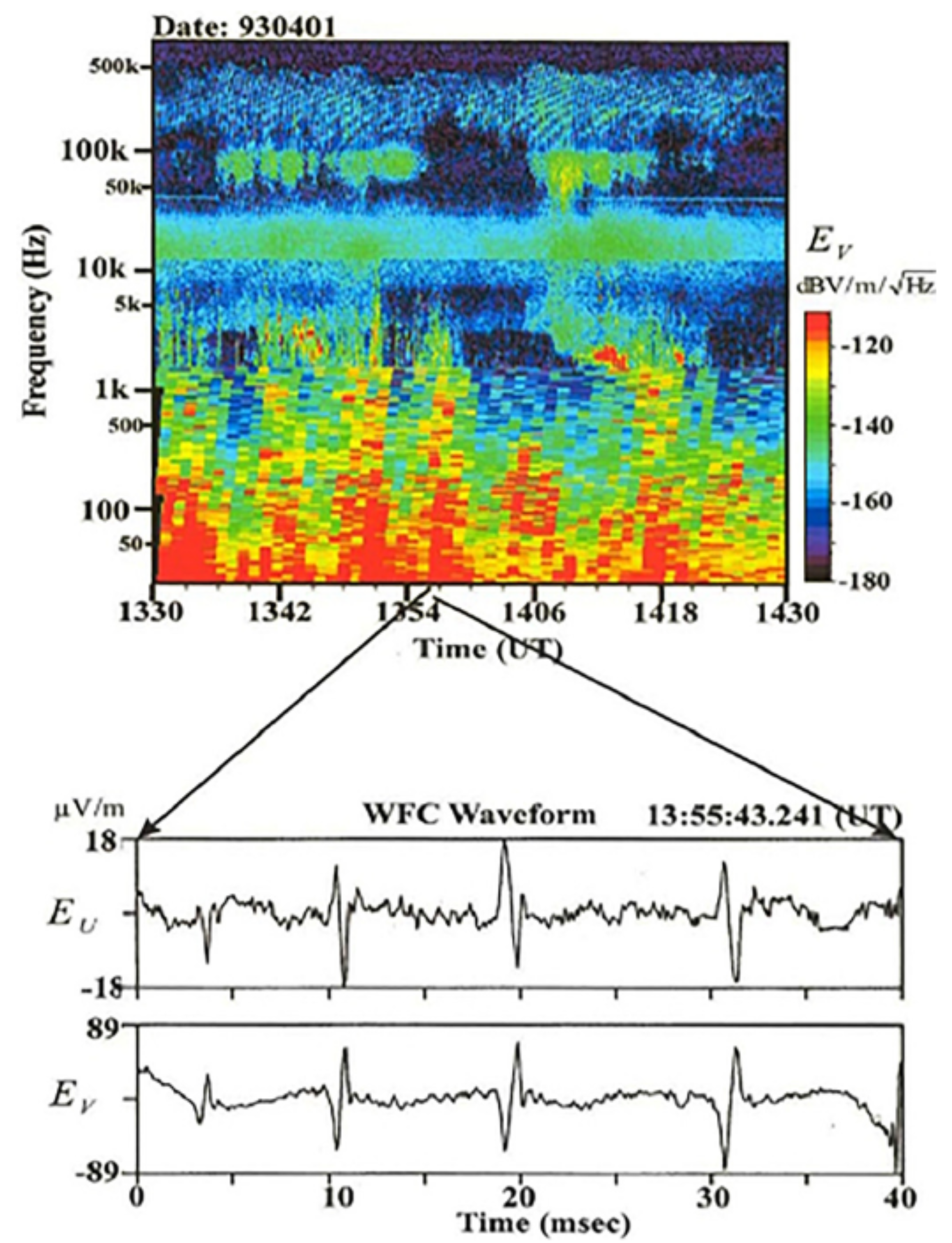
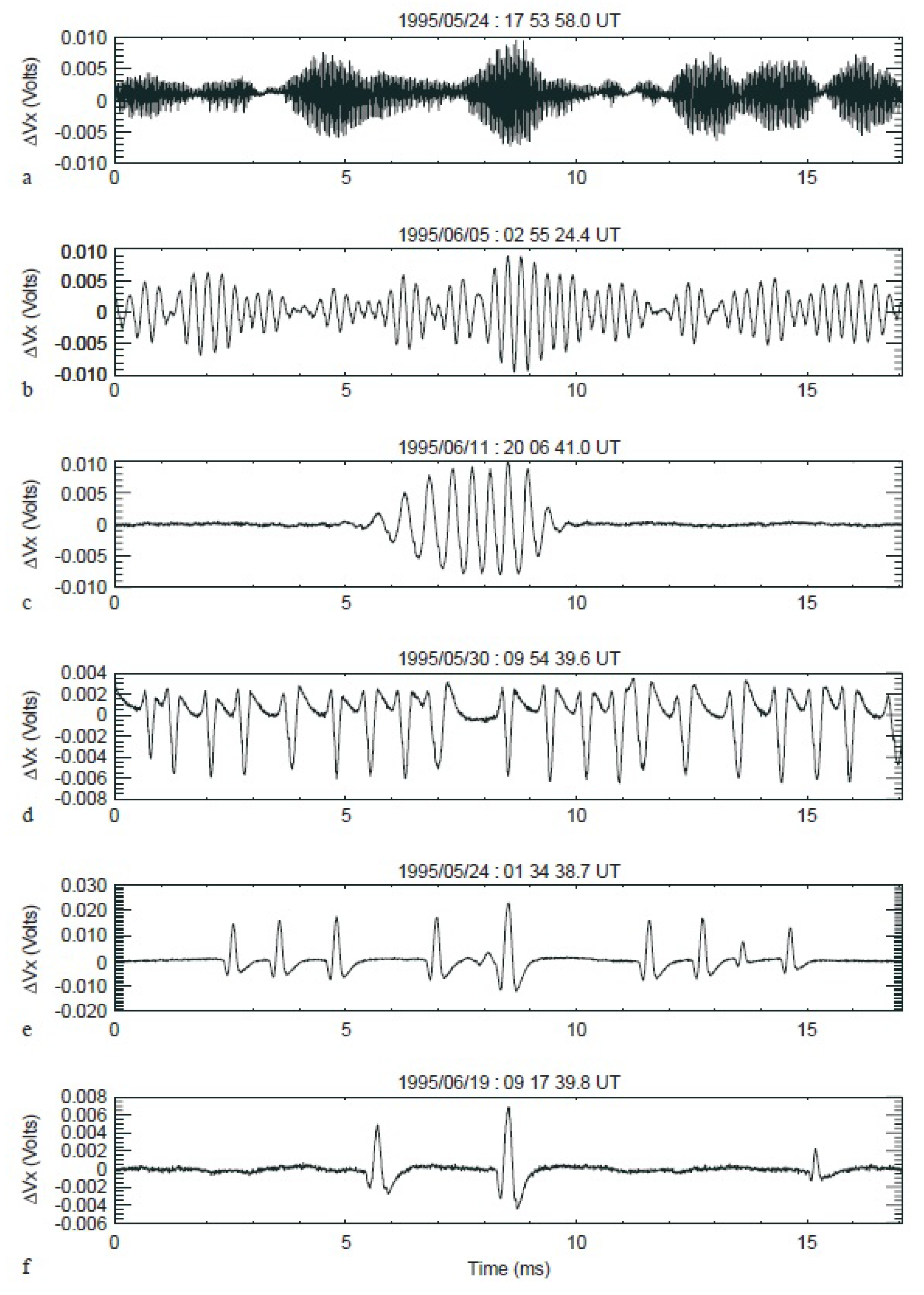
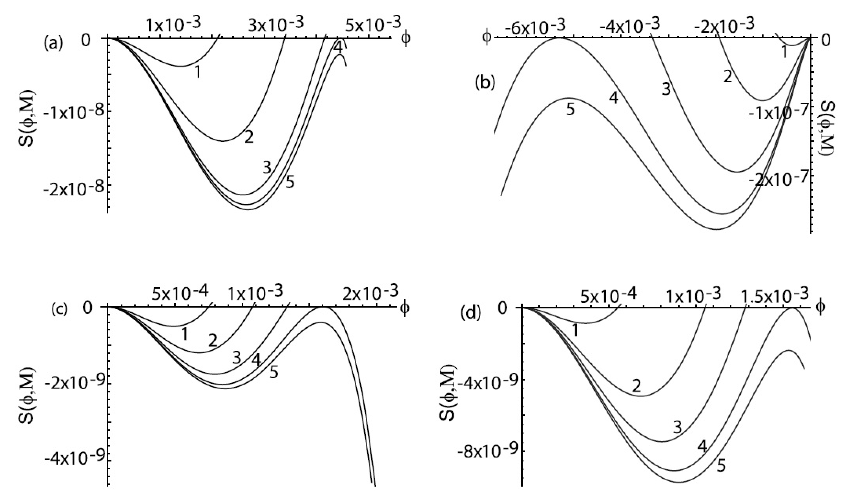
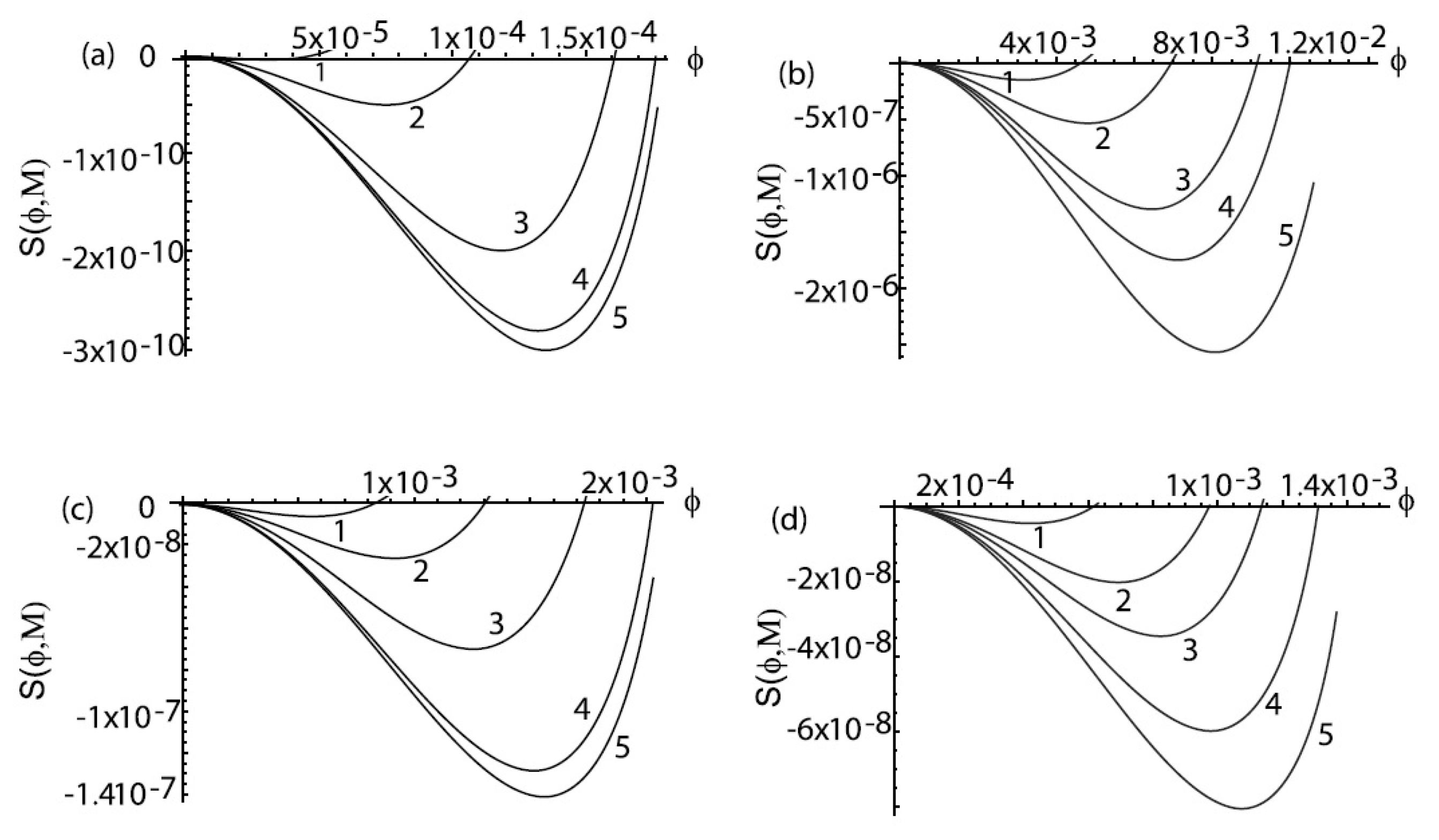
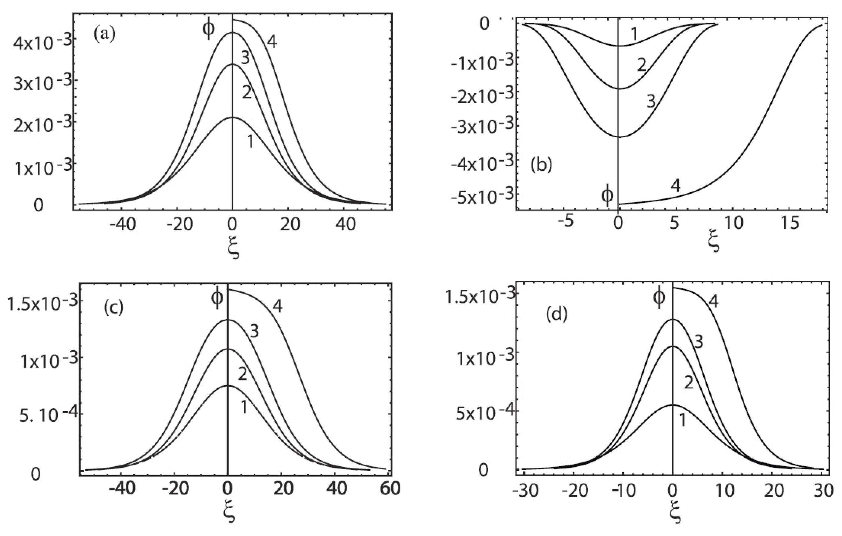
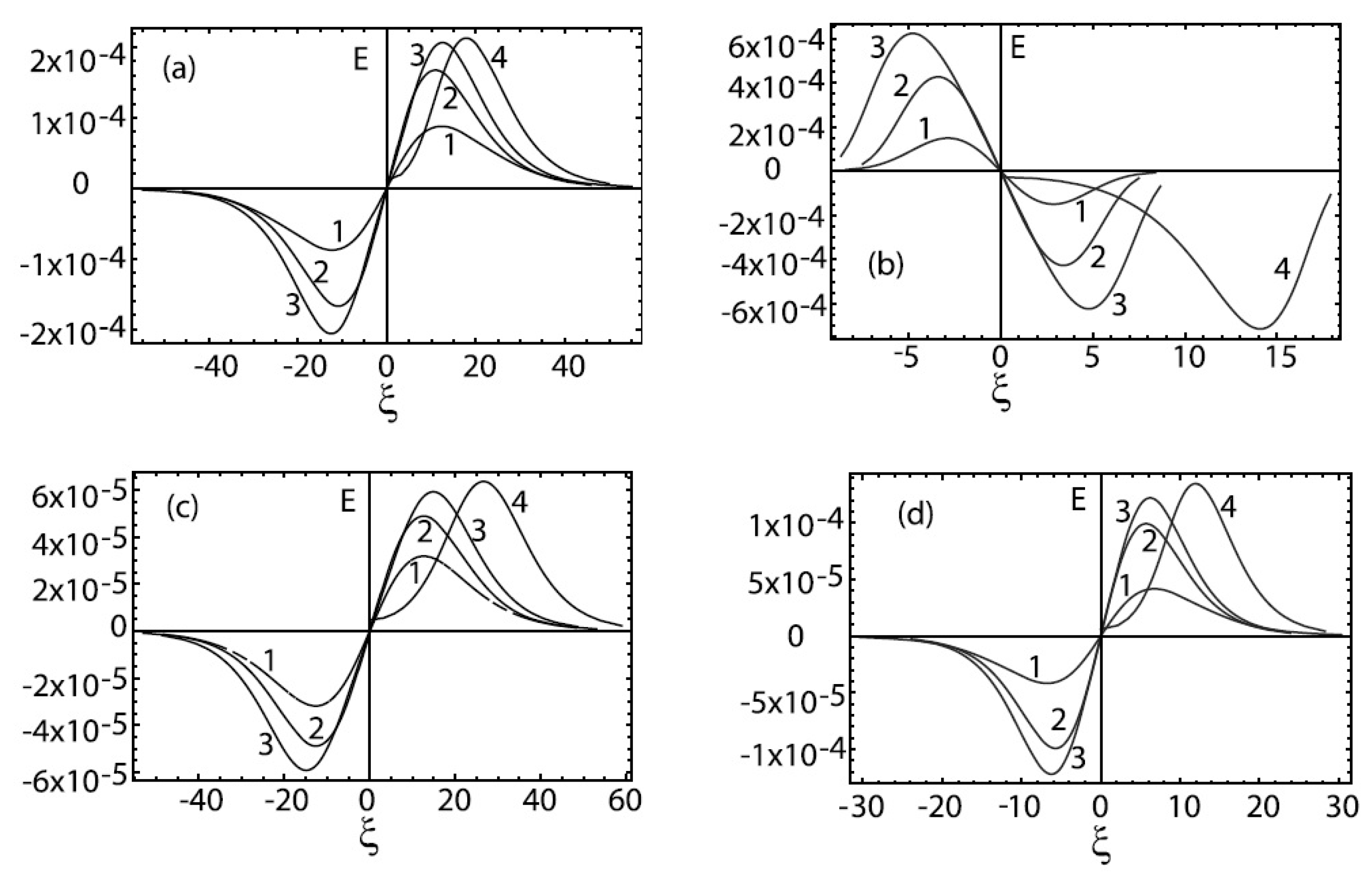
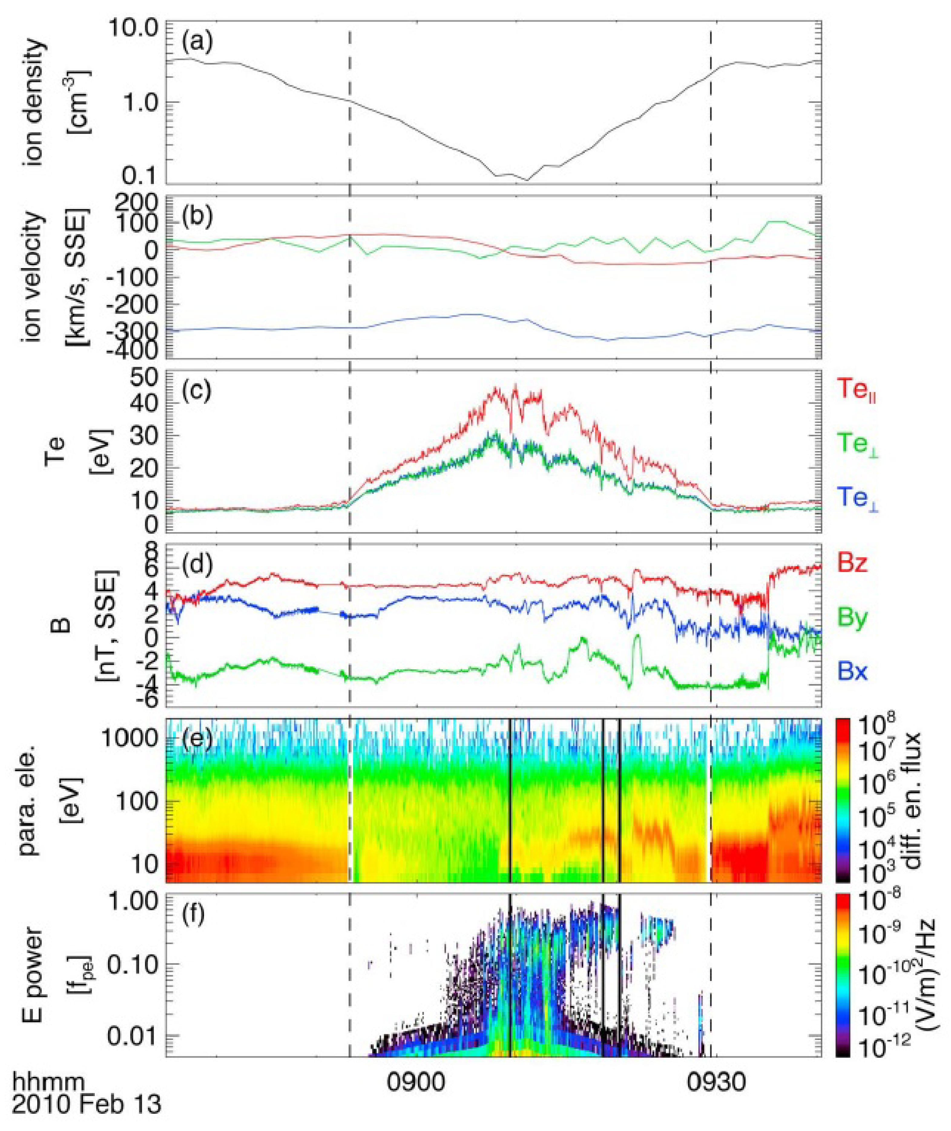
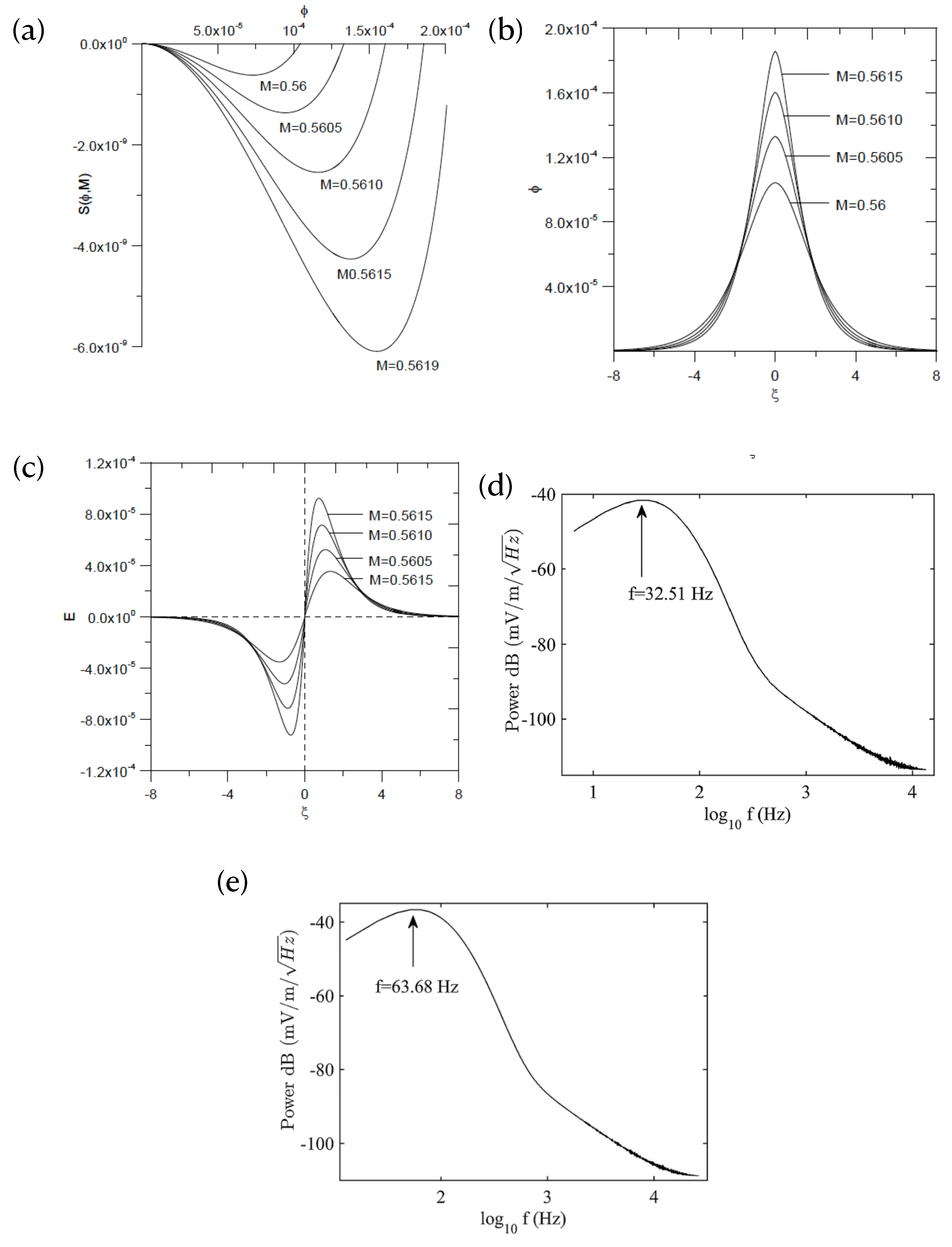
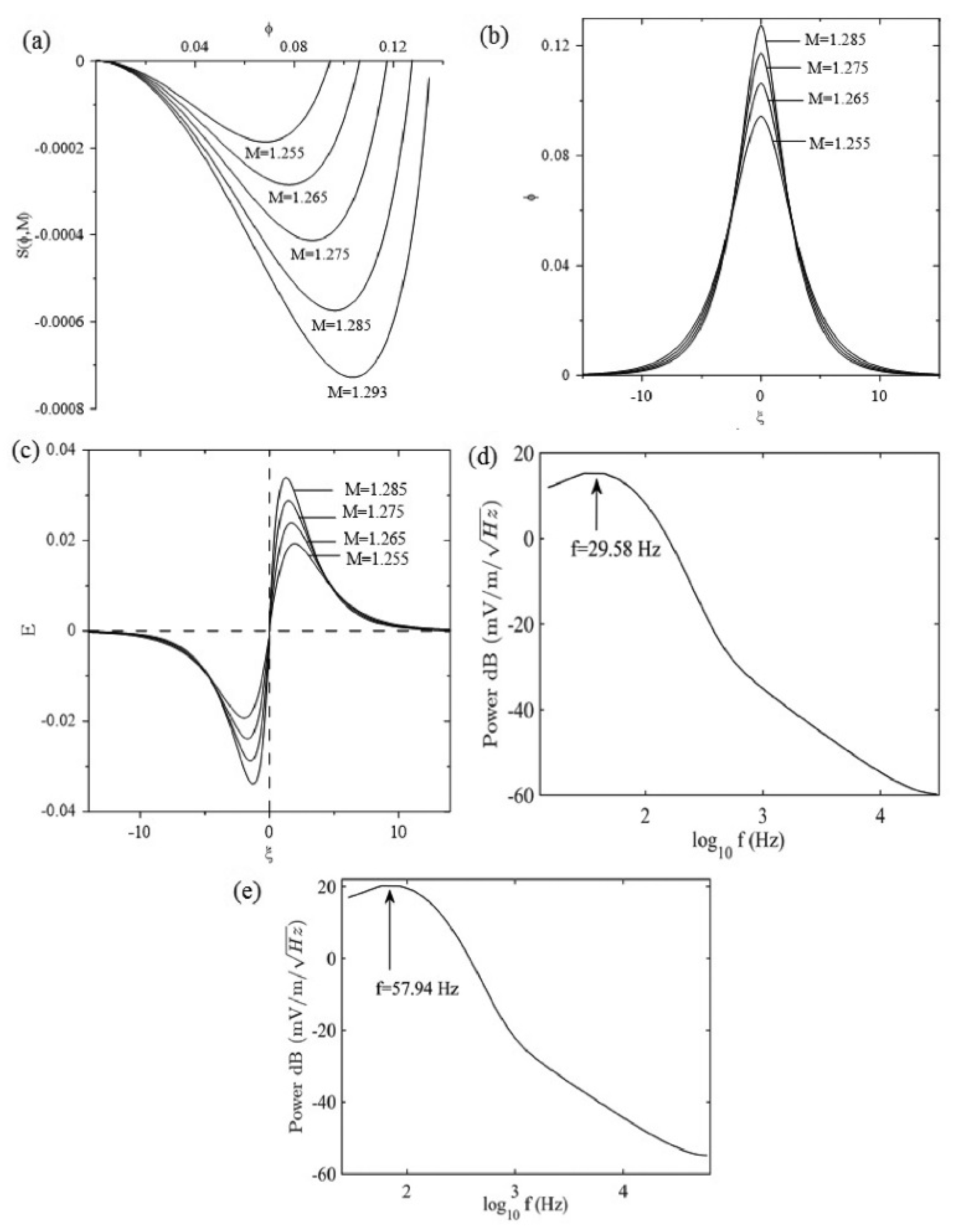
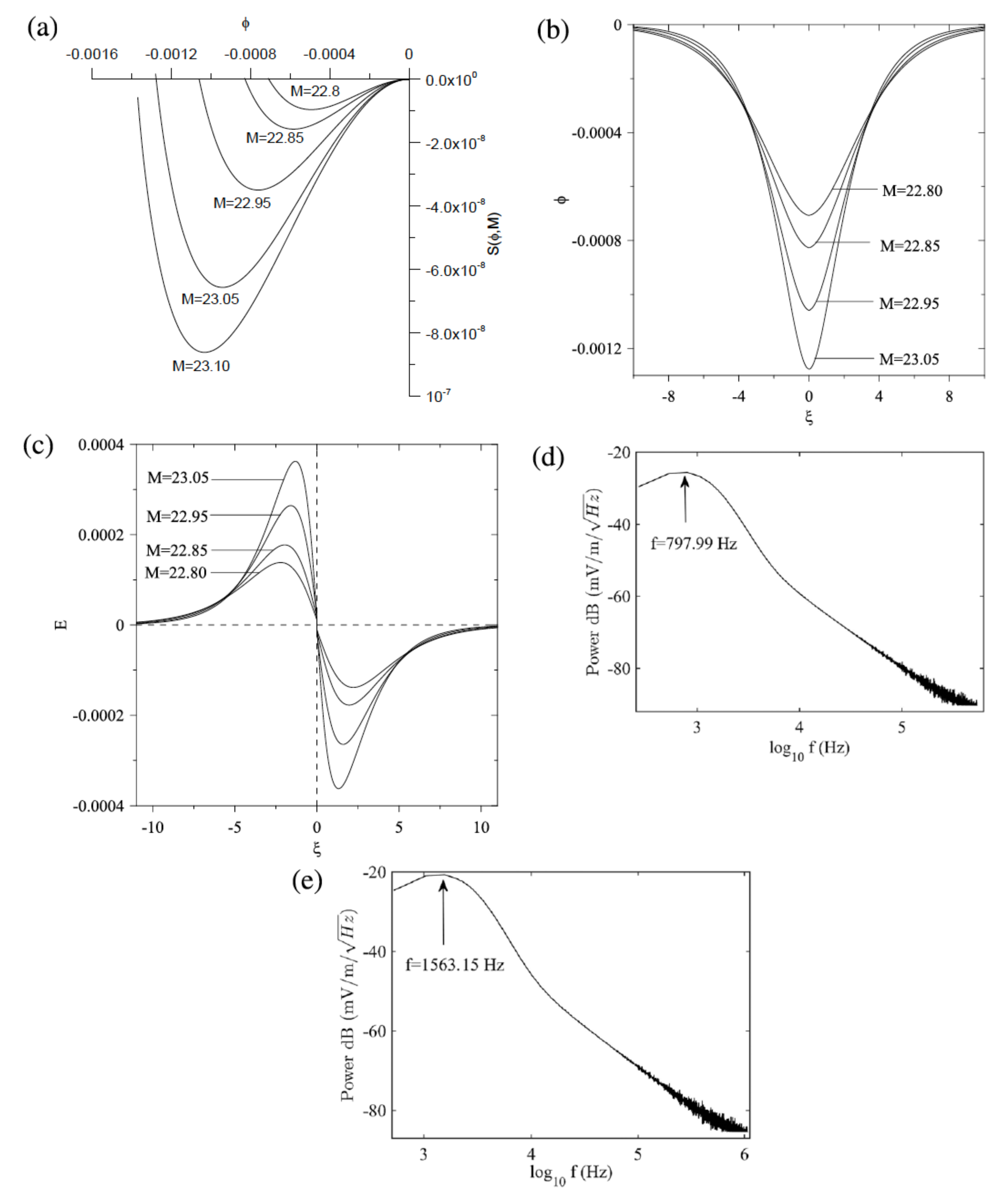
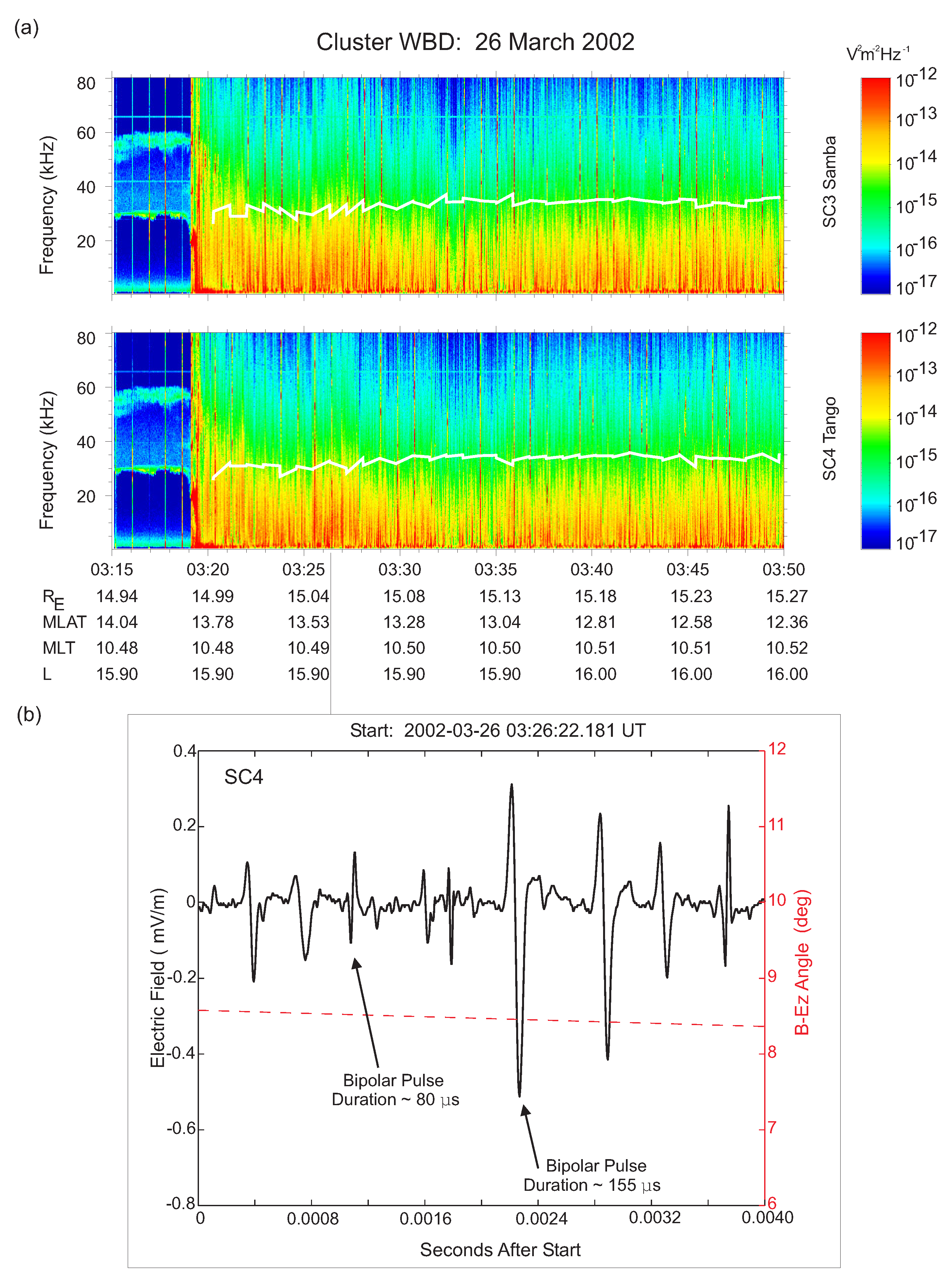
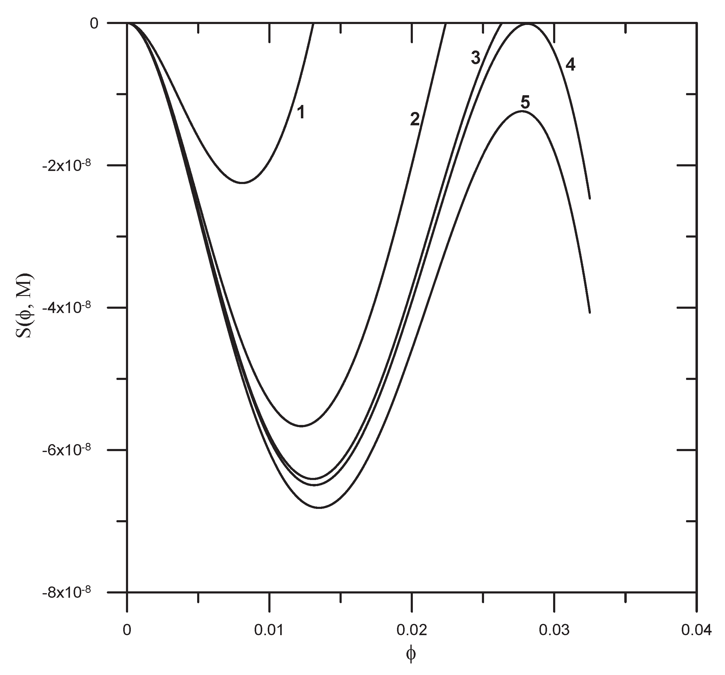
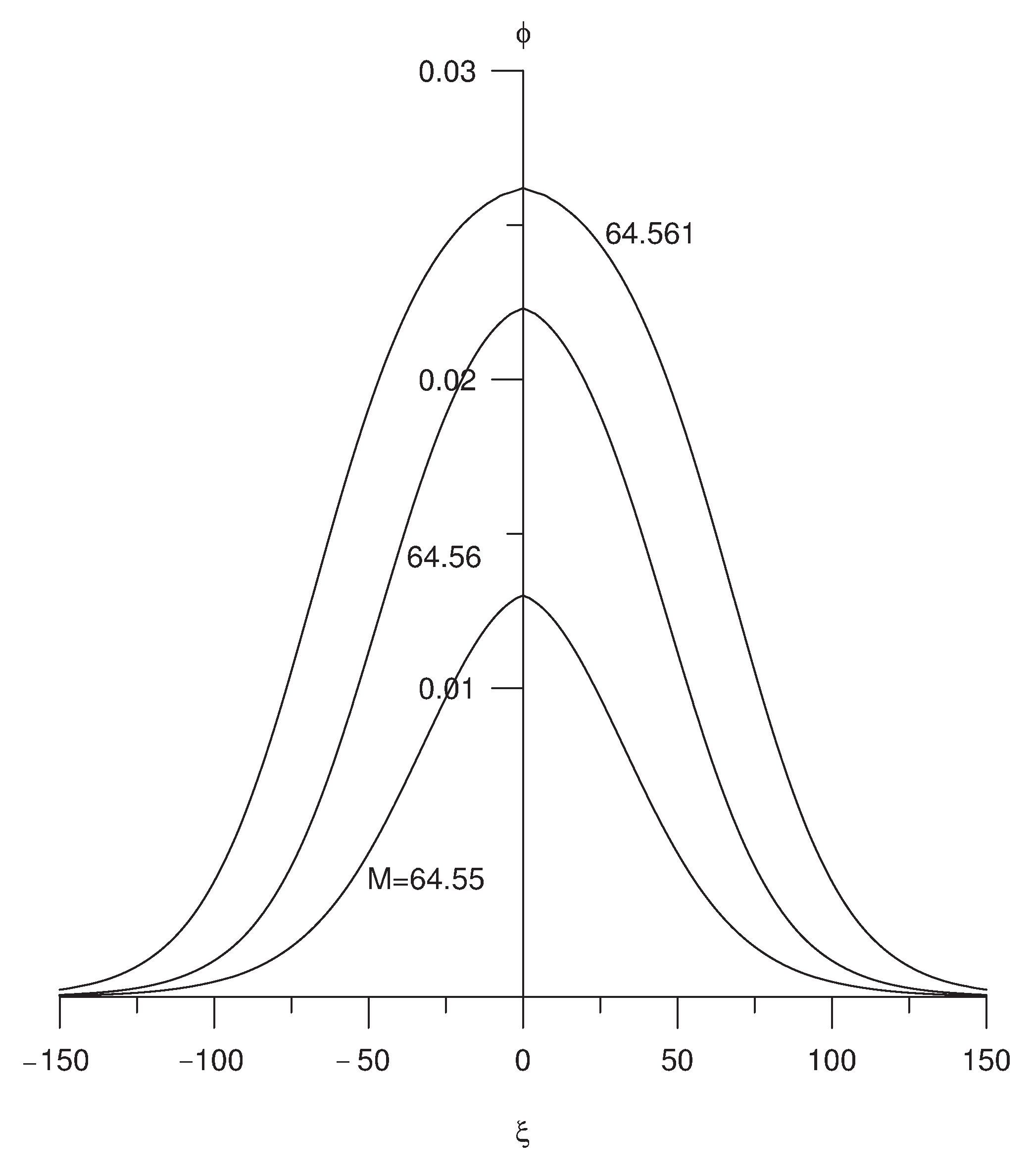
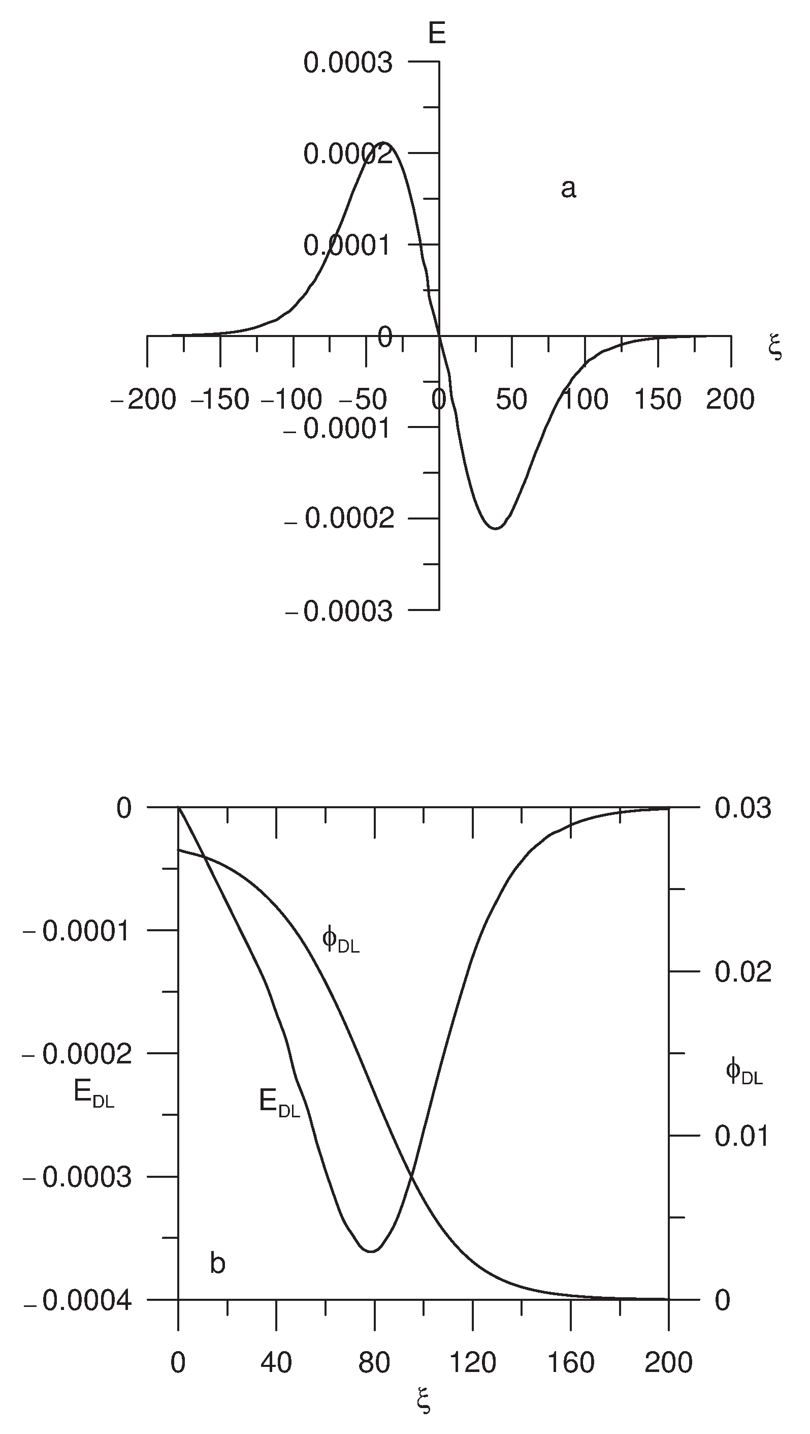
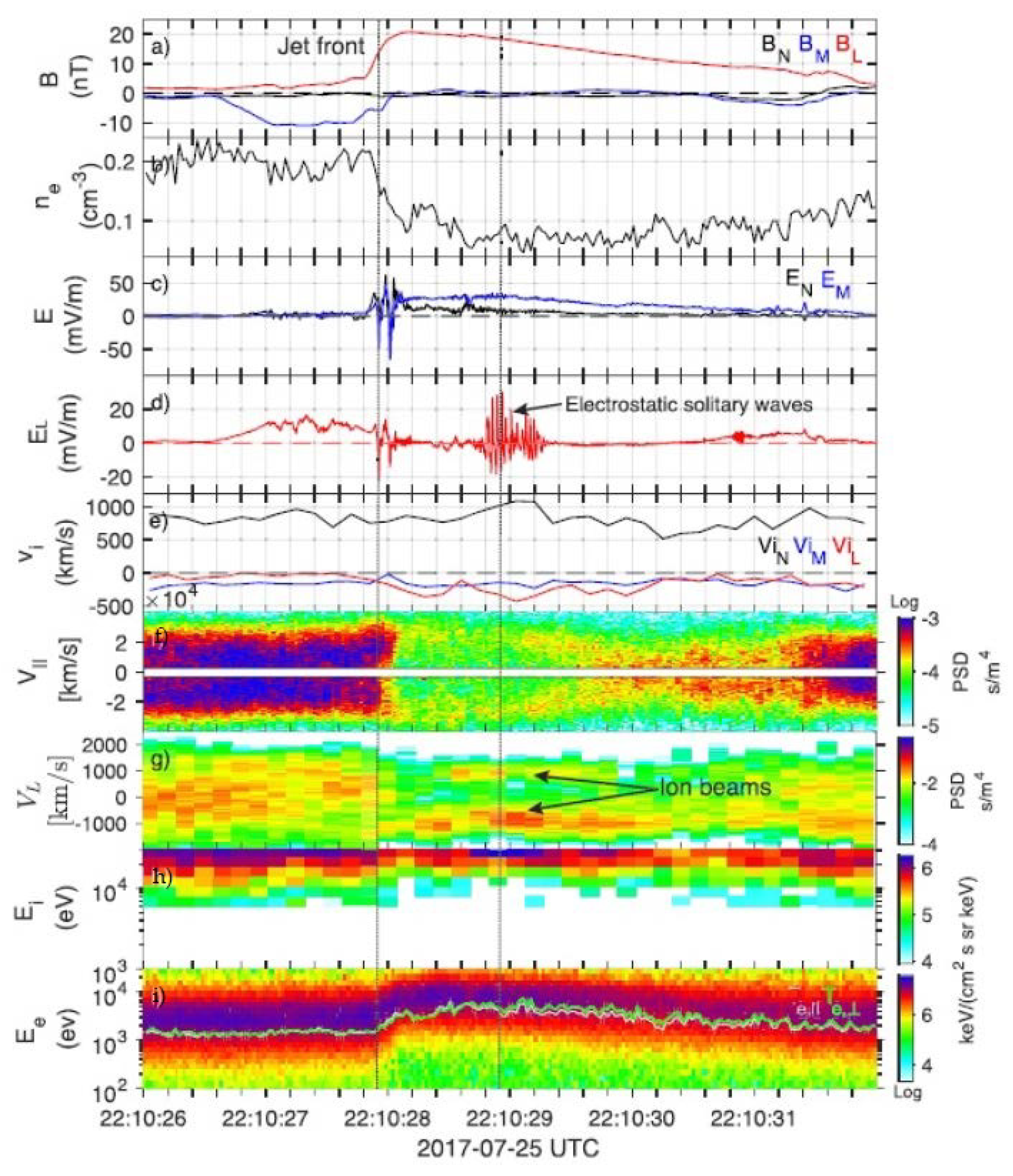
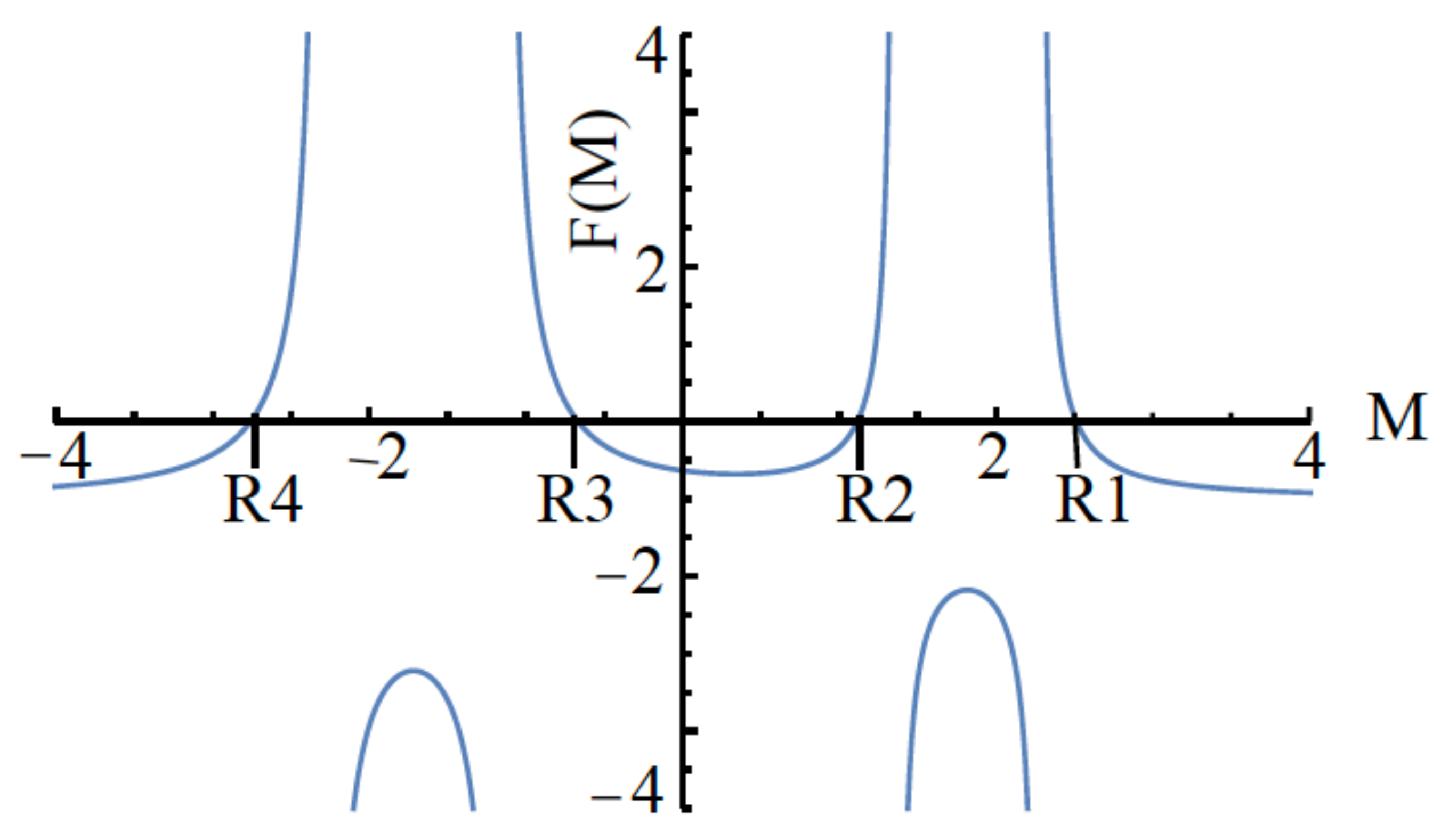
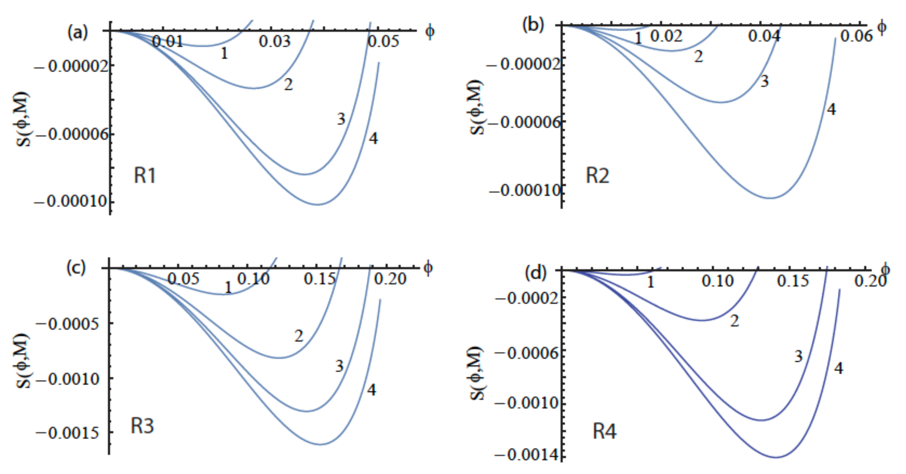
Table 1.
ESWs properties for Run 1 corresponding to WB1 and WB2/WB3. Here, for WB1: —electron temperature, eV, and total equilibrium electron number density, cm, electron plasma frequency, Hz, ion-acoustic speed, C km s, effective hot electron Debye length, m and for WB2/WB3: eV, cm, Hz, C km s, m. Here and in Table 2, V is soliton velocity, E is electric field, W is soliton width and is the frequency of the soliton electric field corresponding to peak power in the spectrum. Reprinted with permission from Rubia et al., J. Geophys. Res. Space Physics, 122, 9134–9147 (2017). Copyright 2017 John Wiley and Sons [182].
| Mode | Polarity | V | E | W | ||
|---|---|---|---|---|---|---|
| (km s) | (mV m) | (m) | (Hz) | |||
| WB1 | Slow ion- | +ve | 28.9– | 0.0003– | 1331– | 6– |
| acoustic | 29.1 | 0.03 | 262 | 34 | ||
| Fast ion- | +ve | 62– | 0.008– | 7439– | 3– | |
| acoustic | 114 | 9.5 | 480 | 41 | ||
| Electron- | -ve | 1169– | 0.004– | 1243– | 262– | |
| acoustic | 1195 | 0.10 | 436 | 803 | ||
| WB2/WB3 | Slow ion- | +ve | 26.0– | 0.0005– | 610– | 13– |
| acoustic | 26.2 | 0.05 | 120 | 67 | ||
| Fast ion- | +ve | 55.6– | 0.02– | 3411– | 5– | |
| acoustic | 60.1 | 16 | 220 | 81 | ||
| Electron- | -ve | 1051– | 0.008– | 570– | 513– | |
| acoustic | 1075 | 0.2 | 200 | 1574 |
Table 2.
ESWs properties for Run 2 corresponding to WB1 and WB2/WB3 parameters listed in Table 1. Reprinted with permission from Rubia et al., J. Geophys. Res. Space Physics, 122, 9134–9147 (2017). Copyright 2017 John Wiley and Sons [182].
| Mode | Polarity | V | E | W | ||
|---|---|---|---|---|---|---|
| (km s) | (mV m) | (m) | (Hz) | |||
| WB1 | Slow ion- | +ve | 28.9 – | 0.0004– | 1222– | 8– |
| acoustic | 29.1 | 0.03 | 240 | 34 | ||
| Fast ion- | +ve | 63.0– | 0.04– | 6501– | 2– | |
| acoustic | 67.3 | 9.7 | 480 | 41 | ||
| Fast ion- | -ve | 63.0– | 0.02– | 8028– | 3– | |
| acoustic | 63.8 | 0.6 | 1113 | 18 | ||
| Electron- | -ve | 1348– | 0.004– | 1200– | 591– | |
| acoustic | 1369 | 0.07 | 436 | 1803 | ||
| WB2/WB3 | Slow ion- | +ve | 26.0– | 0.0008– | 560– | 13– |
| acoustic | 26.1 | 0.05 | 110 | 64 | ||
| Fast ion- | +ve | 56.7– | 0.07– | 2981– | 7– | |
| acoustic | 60.6 | 17 | 220 | 78 | ||
| Fast ion- | -ve | 56.7– | 0.03– | 3681– | 3- | |
| acoustic | 57.4 | 1.0 | 510 | 35 | ||
| Electron- | -ve | 1212– | 0.007– | 550– | 591– | |
| acoustic | 1231 | 0.12 | 200 | 1803 |
Table 3.
Electron properties during observations of magnetosheath solitary waves by Cluster on 26 March 2006 (see Section 8 for description of variables). Reprinted from Lakhina et al., J. Geophys. 114, A09212, 2009. Copyright 2009 John Wiley and Sons [113].
| Event | Time | |||||||||
|---|---|---|---|---|---|---|---|---|---|---|
| hh:mm:ss | cm | eV | km s | cm | eV | km s | cm | eV | km s | |
| 1 | 03:26:00.72 | 6.66 | 45.83 | 11 | 3.00 | 20.69 | 3825 | 2.23 | 14.19 | −4013 |
| 2 | 03:26:12.72 | 6.39 | 47.98 | −50 | 2.74 | 20.68 | 3790 | 2.17 | 14.80 | −4236 |
| 3 | 03:26:16.74 | 6.71 | 48.72 | −6 | 2.82 | 21.98 | 3998 | 2.33 | 15.10 | −4173 |
| 4 | 03:26:24.72 | 6.40 | 47.29 | 42 | 2.88 | 22.69 | 3962 | 1.90 | 12.75 | −4044 |
| 5 | 03:26:32.70 | 6.37 | 51.40 | −70 | 2.63 | 23.76 | 4064 | 1.98 | 15.37 | −4383 |
| 6 | 03:26:40.68 | 6.21 | 52.74 | 21 | 2.52 | 22.38 | 3975 | 1.93 | 15.65 | −4205 |
| 7 | 03:26:48.72 | 6.46 | 53.64 | 50 | 2.58 | 24.49 | 4268 | 1.92 | 16.12 | −4294 |
| 8 | 03:26:52.68 | 6.56 | 54.04 | −42 | 2.41 | 23.15 | 4097 | 1.92 | 16.49 | −4529 |
Table 4.
Properties of electron acoustic solitons and double layers. The highest value of the range under columns 2 to 4 is for the double layer for each event, except for event 8 where the double layer solution does not exist. Reprinted from Lakhina et al., J. Geophys. 114, A09212, 2009. Copyright 2009 John Wiley and Sons [113].
| Event | Range of Allowed | Soliton | Pulse | Electric Field |
|---|---|---|---|---|
| Soliton Velocity | Width | Duration | ||
| V (km s) | W (km) | ( s) | E (mv/m) | |
| 1 | 6125–6127 | 2.5–2.9 | 408–473 | 0.2–1.4 |
| 2 | 6174–6185 | 0.8–1.7 | 133–278 | 1.3–6.5 |
| 3 | 6378–6389 | 0.9–2.1 | 135–330 | 1.3–8.6 |
| 4 | 6319–6321 | 1.7–2.9 | 272–463 | 0.4–1.6 |
| 5 | 6565–6590 | 1.5–1.7 | 230–261 | 0.1–13.2 |
| 6 | 6486–6513 | 1.1–2 | 166–319 | 0.2–14.9 |
| 7 | 6770–6800 | 1.4– 1.9 | 206–276 | 0.2–15.6 |
| 8 | 6667–6740 | 0.6–1.2 | 90–179 | 0.1–35 |
Table 5.
Properties of ion-acoustic solitons corresponding to the reconnection jet parameters (Liu et al., 2019): density of proton beam 1, = 0.026 cm, temperature of proton beam 1, = 300 eV, streaming speed of proton beam 1, = −900 km s, density of proton beam 2, = 0.009 cm, temperature of proton beam 2, = 200 eV, streaming speed of proton beam 2, = 950 km s, electron density, = 0.035 cm, and electron temperature, = 2.86 keV. Then, the ion-acoustic speed is = 523 km s, and Debye length is = 2.12 km. Here, V is the phase velocity, W is the width, E is the electric field, and is the electrostatic potential of the solitons. Reprinted from Lakhina et al., Adv. Space Res, 67, 2021. Copyright 2021 Elsevier [241].
| Roots | Mode | Mach | V (km/s) | W (km) | E (mV/m) | (V) |
|---|---|---|---|---|---|---|
| Number | ||||||
| R1 | Fast ion- | 1334 | 16 | 5 | 70 | |
| acoustic | 1344 | 12 | 11 | 107 | ||
| parallel to | 1355 | 9 | 17 | 138 | ||
| R2 | Slow ion- | 570 | 22 | 3 | 50 | |
| acoustic | 559 | 16 | 7 | 89 | ||
| parallel to | 550 | 12 | 13 | 125 | ||
| R3 | Slow ion- | 15 | 29 | 332 | ||
| acoustic anti- | 11 | 54 | 475 | |||
| parallel to | 9 | 68 | 538 | |||
| R4 | Fast ion- | 21 | 11 | 175 | ||
| acoustic anti- | 13 | 37 | 367 | |||
| parallel to | 9 | 64 | 500 |
Publisher’s Note: MDPI stays neutral with regard to jurisdictional claims in published maps and institutional affiliations. |
© 2021 by the authors. Licensee MDPI, Basel, Switzerland. This article is an open access article distributed under the terms and conditions of the Creative Commons Attribution (CC BY) license (https://creativecommons.org/licenses/by/4.0/).
Share and Cite
MDPI and ACS Style
Lakhina, G.S.; Singh, S.; Rubia, R.; Devanandhan, S. Electrostatic Solitary Structures in Space Plasmas: Soliton Perspective. Plasma 2021, 4, 681-731. https://doi.org/10.3390/plasma4040035
AMA Style
Lakhina GS, Singh S, Rubia R, Devanandhan S. Electrostatic Solitary Structures in Space Plasmas: Soliton Perspective. Plasma. 2021; 4(4):681-731. https://doi.org/10.3390/plasma4040035
Chicago/Turabian StyleLakhina, Gurbax Singh, Satyavir Singh, Rajith Rubia, and Selvaraj Devanandhan. 2021. "Electrostatic Solitary Structures in Space Plasmas: Soliton Perspective" Plasma 4, no. 4: 681-731. https://doi.org/10.3390/plasma4040035