Nonlinear Dynamics of a Single-Mode Semiconductor Laser with Long Delayed Optical Feedback: A Modern Experimental Characterization Approach

Abstract

Semiconductor lasers can exhibit complex dynamical behavior in the presence of external perturbations. Delayed optical feedback, re-injecting part of the emitted light back into the laser cavity, in particular, can destabilize the laser’s emission. We focus on the emission properties of a semiconductor laser subject to such optical feedback, where the delay of the light re-injection is large compared to the relaxation oscillations period. We present an overview of the main dynamical features that emerge in semiconductor lasers subject to delayed optical feedback, emphasizing how to experimentally characterize these features using intensity and high-resolution optical spectra measurements. The characterization of the system requires the experimentalist to be able to simultaneously measure multiple time scales that can be up to six orders of magnitude apart, from the picosecond to the microsecond range. We highlight some experimental observations that are particularly interesting from the fundamental point of view and, moreover, provide opportunities for future photonic applications.

1. Introduction

Semiconductor lasers (SL) have evolved considerably since their introduction in the early 1960s [1,2,3,4]. Nowadays, SL are small and efficient devices regularly used in a variety of applications such as optical data storage, metrology, spectroscopy, material processing, bio-sensing, the pumping of other lasers and optical telecommunications. In particular, its application to long-haul optical data transmission as a high-speed light source has enabled the worldwide optical fiber communication networks.

A characteristic property of most SL is their nonlinear response to perturbations, which manifests itself in a pronounced sensitivity to, e.g., noise, variations in the injection current, external optical injection or delayed optical feedback. This pronounced sensitivity is particularly relevant, as even small amounts of re-injected light can destabilize the SL emission [5,6,7] and induce chaotic dynamics. Even the small back-reflection from an optical fiber tip can destabilize a SL, which is a nuisance for applications in which stable emission is required. The corresponding instabilities are usually prevented via the introduction of optical isolators that shield the laser diode from feedback. Adding optical isolators implies, however, additional costs and complicates the design of compact and miniaturized photonic integrated circuits. The onset of dynamical instabilities was one of the first aspects that was addressed in the study of the nonlinear properties of SL subject to delayed optical feedback [8,9,10,11].

A specific perspective can be adopted when feedback effects are considered from the point of view of nonlinear dynamics. The different dynamical regimes of a delay-coupled SL depend directly on the pump current and feedback parameters, allowing to target specific dynamical regimes by tuning those parameters. The main feedback parameters are the amount of light re-injected into the cavity (feedback rate), the length of the external cavity and the corresponding feedback phase. A SL subject to delayed optical feedback may exhibit many characteristic high-dimensional dynamical phenomena, including hyper-chaotic regimes [12,13] and chaos synchronization when coupled to other SL [14,15]. Moreover, since the complex dynamics generated in delay-coupled SL are exploited in applications as diverse as encrypted communication with synchronized chaotic lasers [16], ultrafast random bit sequence generation [17], light sources with tunable coherence length [18], chaotic LIDAR [19], neuroinspired computation and ultrafast all-optical signal processing [20], a proper experimental and theoretical characterization and understanding are crucial.

The importance of SL subject to delayed optical feedback goes beyond the particular interest in laser dynamics or their photonics related applications. SL are well-controlled and tunable experimental systems, in which we can study nonlinear dynamics phenomena with very high accuracy. Therefore, SL subject to delayed optical feedback are excellent testbed examples of delay-coupled systems in general, being of fundamental importance in a variety of fields. Some examples of these fields are chaos control [21], neuroscience [22], traffic dynamics [23], population dynamics [24], gene regulatory networks [25,26], generic models [27], and secure communications [28].

In this tutorial, we cover some useful experimental tools to characterize the nonlinear dynamics of single-mode SL subject to optical feedback. We focus on the characterization of the intensity dynamics and the corresponding high-resolution optical spectra in the case where the propagation time of the light in the external cavity, i.e., the delay time, is longer than the characteristic time scale of the solitary laser, namely the period of the relaxation oscillations [29].

2. Materials and Methods

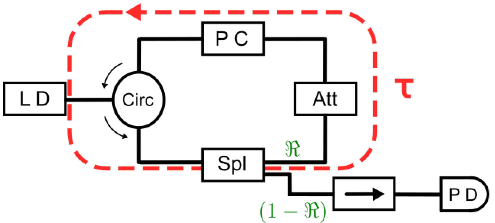
2.1. Experimental Setup

The simplest configuration of delayed optical feedback comprises a SL diode and an optical reflector, which could be provided, e.g., by a mirror. Figure 1 shows a schematic view of such an experimental set-up, where the feedback is implemented as a loop via optical fibers. We consider a SL diode that emits stably in a continuous wave operation when unperturbed. The feedback loop redirects a fraction ${\kappa }_f$ of the laser’s emitted optical field back into the laser cavity after a delay time $\tau$. The properties of the laser emission depend on the amount of light that is reinjected into the laser [9]. Here, we will show experimental results for Discrete-Mode Laser-Diodes that have a Fabry–Perot structure with etched and longitudinally periodic ridges, which have been designed such that they yield single longitudinal-mode operation for a wide range of operating conditions [30]. The discrete-mode laser diode discussed in the following emits at a wavelength of about 1542 nm. The SL used in the following did not include an optical isolator in its butterfly packaging.

The first and most straightforward consequence of delayed optical feedback that can be measured in SL is its effect on the output power. Coherent optical feedback typically reduces the lasing threshold as compared to solitary operation. This threshold reduction is due to photons being re-injected into the laser cavity, reducing the total optical losses. Figure 2 displays two different power-current characteristics of the same laser under different experimental conditions. The blue curve corresponds to the case of the SL without feedback, in comparison to which the presence of delayed optical feedback reduces the SL’s threshold current, see the orange curve. By means of measuring the relative losses through the successive elements in the external cavity, a maximum value of the feedback rate can be estimated. The maximum feedback rate, i.e., the fraction of intensity reflected back to the laser diode for this particular setup is 54%, excluding the laser and fiber-coupling losses. The kink in the feedback power-current characteristics is due to the appearance of low frequency fluctuations dynamics close to the solitary lasing threshold.

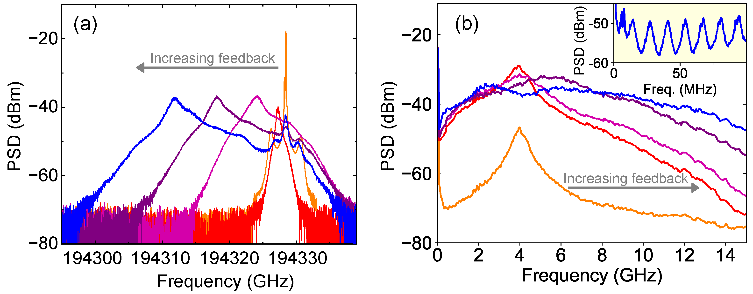
2.2. Spectral Characterization of Feedback-Induced Dynamics

Since the lasing threshold is reduced, temporally averaged input–output characteristics draw a rather positive image of delayed optical feedback. From the viewpoint of the intensity dynamics of the laser, however, delayed feedback has a much more ambiguous effect. In fact, since the early days of SL, feedback was considered a clear nuisance for their operation as it created power instabilities and increased the laser’s spectral bandwidth [5,6,7], i.e., reducing its coherence.

Figure 3 illustrates this optical feedback-induced broadening on the optical and radio-frequency power spectra. Figure 3a depicts the optical spectra as measured with a high-resolution optical spectrum analyzer (resolution 10 MHz). Different colors correspond to different feedback rates, with the orange curve plotting the solitary laser spectrum and the blue color plotting the highest feedback rate. In this figure, the higher the value of the feedback rate, the broader the optical spectrum becomes, mostly broadening towards lower frequencies, that is, longer wavelengths. For the highest feedback rates on this particular device, the broadening of the spectrum already covers more than 20 GHz. This well known phenomenon is frequently referred to in the literature as coherence collapse [8]. For an even higher feedback rate, the SL can eventually become stable again with a reduced linewidth [31].

A complementary spectral characterization tool for the experimentalist is the radio frequency (RF) power spectrum of the emitted light intensity. Figure 3b depicts the impact of delayed optical feedback on the RF power spectrum, providing additional information complementary to that present in the optical domain. On a multi-GHz scale, one can observe a clear broadening of the RF spectrum due to the feedback. The relaxation oscillations frequency is visible for the solitary laser around 4 GHz (frequency with the highest power density for the orange curve), a feature that is typically observed in the relative intensity noise spectrum of class B lasers [32]. Increasing the feedback rate results in a broadening of the RF spectrum with its maximum shifting towards higher frequencies. Colors for the different feedback scenarios correspond to those of the optical spectra, with blue representing the highest feedback rate. The inset in Figure 3b depicts the fingerprint of the delay time in the RF power spectrum. The visible resonances in the RF power spectrum are separated roughly by the inverse of the light flight time in the external cavity. The resonance separation is here 13.29 MHz, yielding an approximate value of the external cavity delay, here ($\tau$ ≈ 75 ns) [33]. An experimental method to measure the delay time more precisely is to induce an optical pulse with a steep slope (small rise time) and to measure the time intervals between multiple reflections in the external cavity [33].

The linewidth enhancement factor ($\alpha$), characteristic for SL, plays a crucial role in the destabilization of the laser emission via delayed optical feedback that ultimately leads to the collapse of the optical coherence. This parameter accounts for the coupling between light intensity and optical phase [34]. As a consequence, any intensity fluctuation in the laser’s emission will be fed-back via the delay path, re-enter the gain medium, and affect intensity and optical phase.

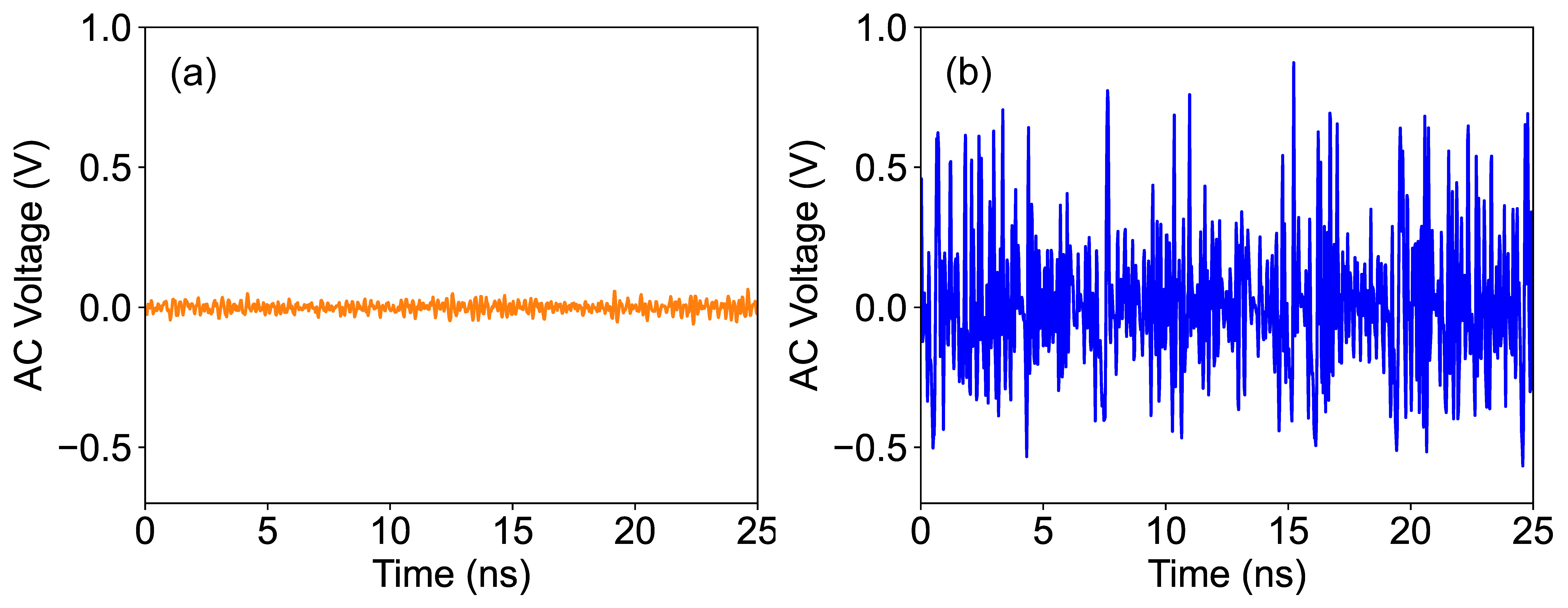
2.3. Temporal Characterization of Feedback-Induced Dynamics

Figure 4 illustrates the impact of delayed optical feedback on the temporal emission characteristics of SL. The solitary emission is depicted in Figure 4a, where the AC-coupled intensity time series shows small fluctuations around the origin. Those intensity fluctuations are the combination of amplified spontaneous emission and detection noise, particularly when the laser is biased close to the threshold. The corresponding optical linewidth depends on the optical power and for the operating conditions in Figure 4a is approximately 1 MHz. In contrast, in Figure 4b, the irregular emission behavior under delayed optical feedback is illustrated. The intensity dynamics exhibits chaotic pulsations on a sub-ns time scale. The optical spectrum corresponding to such dynamics expands the SL’s linewidth from ∼1 MHz to tens of GHz. The detection bandwidth plays a fundamental role in the study of the intensity dynamics of the SL subject to optical feedback. The fast intensity pulsations, which remained mostly unresolved until first measured with a streak camera [35], can now be characterized in detail due to oscilloscopes with several tens of GHz analog bandwidth in combination with fast photodetectors.

While it is, meanwhile, possible to fully resolve the complex intensity dynamics exhibited by delayed feedback lasers, a direct inspection of chaotic time series is of restricted help for understanding how the dynamics depends on the different system parameters. Here, choosing an appropriate representation of the measured time series is key. Figure 5 illustrates two useful methods to represent features of the time-resolved intensity dynamics in a comprehensive and informative way. Figure 5a depicts the autocorrelation function (ACF) of the intensity dynamics. The most characteristic signature of delayed dynamics is present in the revival peaks located at multiples of the delay time. The inset in Figure 5a zooms on the first ACF peak at a lag time of ∼$\tau$. The spatio-temporal representation of the intensity dynamics is shown in Figure 5b. In this two-dimensional representation, inspired by the two main timescales in the ACF, delay time intervals are plotted as a pseudo-space variable [36]. Here, the abscissa denotes the time offset in a delay interval of length $\tau$, while the vertical axis denotes the ordinal of the current delay interval. In this manner, the intensity time series is divided in temporal segments of length $\tau$ and consecutive segments are then plotted on top of each other. For instance, the bottom line in Figure 5b corresponds to time $0\le t<\tau$ in the original time-series, the line directly above corresponds to time $\tau \le t<2\tau$, and so on. The intensity of the laser is encoded in grey-scale. From such a representation, specific information can be extracted from a long time series, in particular if the plotted dynamics is irregular or chaotic [37].

2.4. Theoretical Background

The results reported in this tutorial have been obtained in experiments using quantum well single mode laser diodes. Even though these results are model-independent, it is of major interest to link these findings with existing numerical models. A SL subject to moderate optical feedback can in many cases be described by the Lang–Kobayashi rate equations as follows [38]:

$$\begin{array}{cc}\hfill \frac{dE\left(t\right)}{dt}& =\frac{1+\mathrm{i}\alpha }{2}\left[G_{\mathrm{N}}(N\left(t\right)-N_o)-\frac{1}{{\tau }_p}\right]E\left(t\right)+\kappa E(t-\tau )e^{-\mathrm{i}2\pi f_{th}\tau },\hfill \end{array}$$

(1)

$$\begin{array}{cc}\hfill \frac{dN\left(t\right)}{dt}& =\frac{I}{e}-\frac{N\left(t\right)}{{\tau }_s}-G_{\mathrm{N}}(N\left(t\right)-N_o){\left|E\left(t\right)\right|}^2,\hfill \end{array}$$

(2)

where E and N are the complex electric field amplitude and the carrier number, respectively. The main feedback parameters, namely the delay time $\tau$ and the feedback rate $\kappa$, can be seen in Equation (1). Other parameters in Equation (1) are the linewidth enhancement factor $\alpha$, the differential optical gain $G_{\mathrm{N}}$, the carrier number at transparency $N_o$, the photon lifetime ${\tau }_p$, and the laser solitary frequency at lasing threshold $f_{th}$. In Equation (2), I is the pump current, e the electron charge, and ${\tau }_s$ is the carrier lifetime.

For a detailed analysis of the Lang–Kobayashi model, we refer the reader to the existing literature [10,39]. Here, we will focus on the steady-state solutions of Equations (1) and (2). since they provide the backbone of the observed dynamical phenomena.

2.4.1. External Cavity Modes

The relative equilibria solutions for the SL subject to optical feedback can be obtained by introducing $P\left(t\right)={\left|E\left(t\right)\right|}^2=P_s$, $N\left(t\right)=N_s$, and ${\varphi }_s\left(t\right)=2\pi (f_s-f_{th})t$ in Equations (1) and (2). Here, $\varphi \left(t\right)$ denotes the phase of the electric field $E\left(t\right)$, while $P_s$, $N_s$ and $f_s$ are constant. Accordingly, the steady-state solutions read:

$$\begin{array}{cc}\hfill N_s& =N_{th}-2\frac{\kappa }{G_N}cos\left(2\pi f_s\tau \right),\hfill \end{array}$$

(3)

$$\begin{array}{cc}\hfill 2\pi (f_s-f_{th})& =\kappa \sqrt{1+{\alpha }^2}sin(2\pi f_s\tau +\arctan \left(\alpha \right)),\hfill \end{array}$$

(4)

$$\begin{array}{cc}\hfill P_s& =\frac{\frac{I}{e}-\frac{N_s}{{\tau }_s}}{G_N(N_s-N_o)},\hfill \end{array}$$

(5)

where $N_{th}=N_o+1/\left({\tau }_p{G}_N\right)$. The solutions in Equations (3)–(5) are rotating waves, which lie on an ellipse in the ($f_s$, $N_s$) plane [40,41]. Figure 6 shows such ellipses of relative equilibria obtained for different parameter values of the feedback rate, delay time, and linewidth enhancement factor. The external cavity modes (ECM) are the solutions that originate from constructive interference between the laser field and the delayed feedback, blue circles in Figure 6, while the external cavity antimodes are the ones corresponding to destructive interference and are shown as orange triangles in Figure 6.

As illustrated in Figure 6, the maximum feedback-induced frequency shift in the Lang–Kobayashi model is approximately $\mathsf{\Delta }{f}_{fb}=\alpha \kappa /2\pi$ (extremes of the ellipse) and the frequency separation between ECM is proportional to ${\tau }^{-1}$, where $f_{EC}={\tau }^{-1}$ is the frequency associated to the external cavity. Thus, the extent of the ellipse is $\mathsf{\Delta }{f}_{fb}\sim$ 6.35 GHz in Figure 6a,b, while $\mathsf{\Delta }{f}_{fb}\sim 12.7\mathrm{GHz}$ in Figure 6c, respectively. In turn, the separation between the ECMs is ${\tau }^{-1}\sim 1\mathrm{GHz}$ in Figure 6a,c, while ${\tau }^{-1}\sim 0.5\mathrm{GHz}$ in Figure 6b, respectively. The eccentricity of the ellipse of external cavity modes and antimodes is determined by $\alpha$.

To understand the feedback-induced laser dynamics, the relaxation oscillation frequency of the solitary laser is of great relevance. The relaxation oscillation frequency of the solitary laser, i.e., Equations (1) and (2) with $\kappa =0$, is given by $f_{RO}=\frac{1}{2\pi }\sqrt{G_{\mathrm{N}}(I-I_{th})/e}$, where $I_{th}$ is the pump current at the lasing threshold. As will be shown in Section 3, the relationship between $\mathsf{\Delta }{f}_{fb}$ and $f_{RO}$ plays a major role in the observed dynamics of the SL subject to optical feedback since we are dealing with an experimental system with a large delay ($\tau$ ≈ 75 ns).

3. Experimental Results: Dynamical Regimes

Spectral and dynamical phenomena in delayed feedback SL depend on the combination of both, laser and feedback parameters. It is possible, however, to group these intricate dependencies in different scenarios or feedback regimes. Here, three characteristic experimental scenarios are analyzed, corresponding to different degrees of influence of feedback on the single laser behavior. In the following, feedback rate and bias current are the two parameters varying between low, intermediate and strong feedback scenarios.

As illustrated in [42], feedback regimes depend mainly on the relation between the system’s three principal frequencies: the relaxation oscillations frequency $f_{RO}$, the external cavity frequency $f_{EC}$, and the feedback-induced frequency shift $\mathsf{\Delta }{f}_{fb}$, respectively. The dynamical characteristics, shown for a given combination of feedback and laser parameters, are similar to any other combination of parameters that keep the ratios $f_{RO}$/$\mathsf{\Delta }{f}_{fb}$ and $f_{RO}$/$f_{EC}$ constant. As discussed in Section 2.4.1, $f_{RO}$ depends on bias current I and $\mathsf{\Delta }{f}_{fb}$ on feedback rate $\kappa$. The particular values of the three bias currents and feedback rates in the following were chosen to best illustrate the dynamic and spectral characteristics of feedback-induced semiconductor laser dynamics in the low, intermediate and strong feedback regimes, respectively. By working in the limit of long external cavities, with $f_{RO}\gg f_{EC}$, the ratio $f_{RO}$/$\mathsf{\Delta }{f}_{fb}$ dominates the global dynamics, while the ratio $f_{RO}$/$f_{EC}$ determines if the temporal dynamics is contracting or expanding [42].

The experimentally measured transition between the three feedback conditions shown here does not necessarily visit discrete feedback regimes, but rather features continuous transitions between these. A description of such dependence and their relation with the system’s time scales can be found in [42]. For a detailed study of the bifurcation-cascade diagrams in delayed feedback lasers we refer, e.g., to this previous work [43].

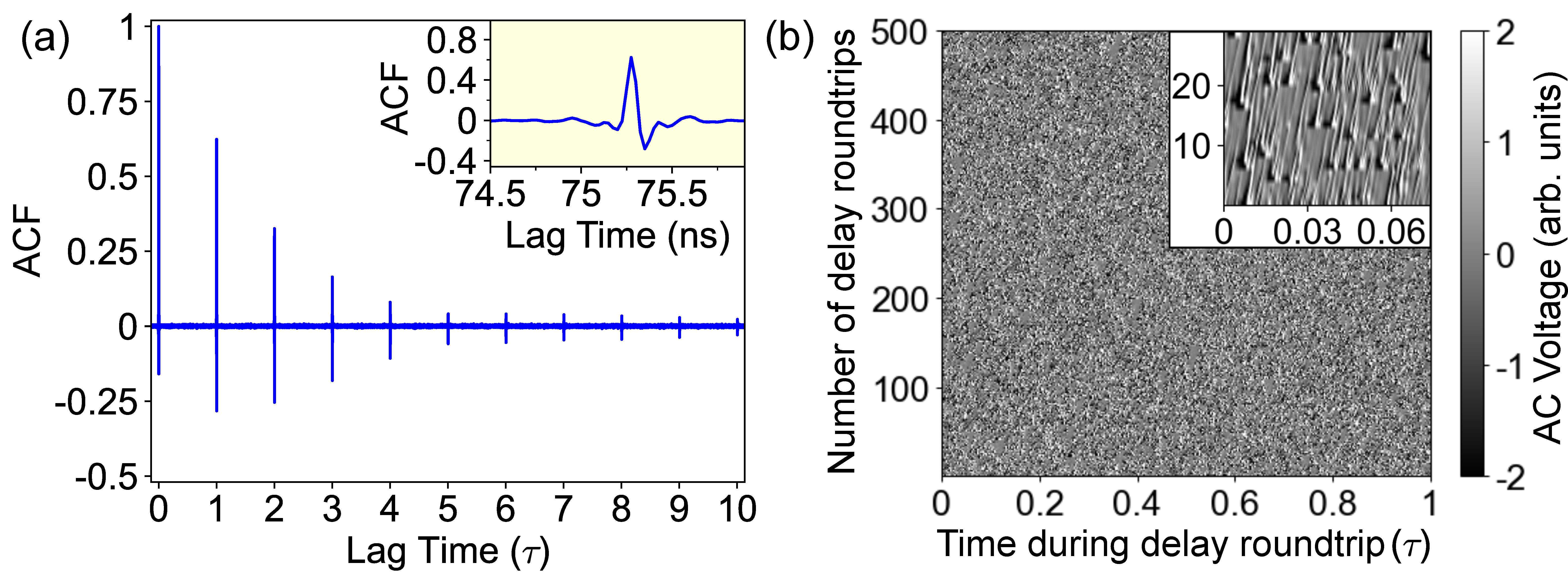
3.1. Low Feedback Rate

The first illustrated regime corresponds to the weakest feedback condition, the onset region of dynamical instabilities. In the selected example, the bias current I = 18 mA is approximately $\simeq 1.5{\mathrm{I}}_{\mathrm{th}}$ and the feedback rate has been strongly attenuated by 31 dB from its maximum value. This combination of bias current and feedback rate leads to the condition $f_{RO}>\mathsf{\Delta }{f}_{fb}$. In particular, the chosen parameter values correspond to undamped relaxation oscillations dynamics [44], occurring just after the destabilization of the solitary laser emission.

Figure 7a shows the optical spectrum, which is characterized by the presence of sharp well defined peaks at left and right sides of the solitary laser mode ($f_{SOL}$). The frequency peak at its immediate left side corresponds to the feedback-induced frequency shift ($\mathsf{\Delta }{f}_{fb}$). In addition, one can observe several side peaks that are shifted by multiples of the relaxation oscillation frequency ($f_{RO}$). This is the signature of the undamping of the relaxation oscillations. Such resonances are clearly identifiable in the RF spectrum depicted in Figure 7b. As shown in Figure 7a, $\mathsf{\Delta }{f}_{fb}$ is smaller than the relaxation oscillations frequency $f_{RO}$ for this weak feedback regime.

The ACF is depicted in Figure 7c for an interval of $10\tau$. The overall ACF decay along multiple delay echoes is very small and the system contains, on average, persistent $\tau$-feedback memory of its past states. The inset in Figure 7c depicts the ACF oscillations around the first delay echo. These oscillations are the signature of the undamped relaxation oscillations in the ACF and are dominated by $f_{RO}$, as visible in the RF spectrum. In the broader view of the ACF, a particular lobe structure modulates the ACF envelope amplitudes in between delay echoes. Only a slight modification of any of the feedback parameters can significantly modify the lobe structure, but their influence on the ACF height will be minor.

Figure 7d illustrates the spatio-temporal representation of the intensity dynamics. This representation clearly elicits the high correlation of the local dynamics with the delay time $\tau$. For a time window of $500\tau$ (more than $30\mathsf{\mu }\mathrm{s}$), two distinct and separate dynamical behaviors—namely stable emission and an oscillatory state—coexist. The region magnified in the inset allows the identification of oscillations of constant frequency $f_{RO}$ that characterize the oscillatory region and a sharp transition to the stable regime. The coexistence of stable and unstable dynamics is a common feature of SL with low optical feedback [43,45,46].

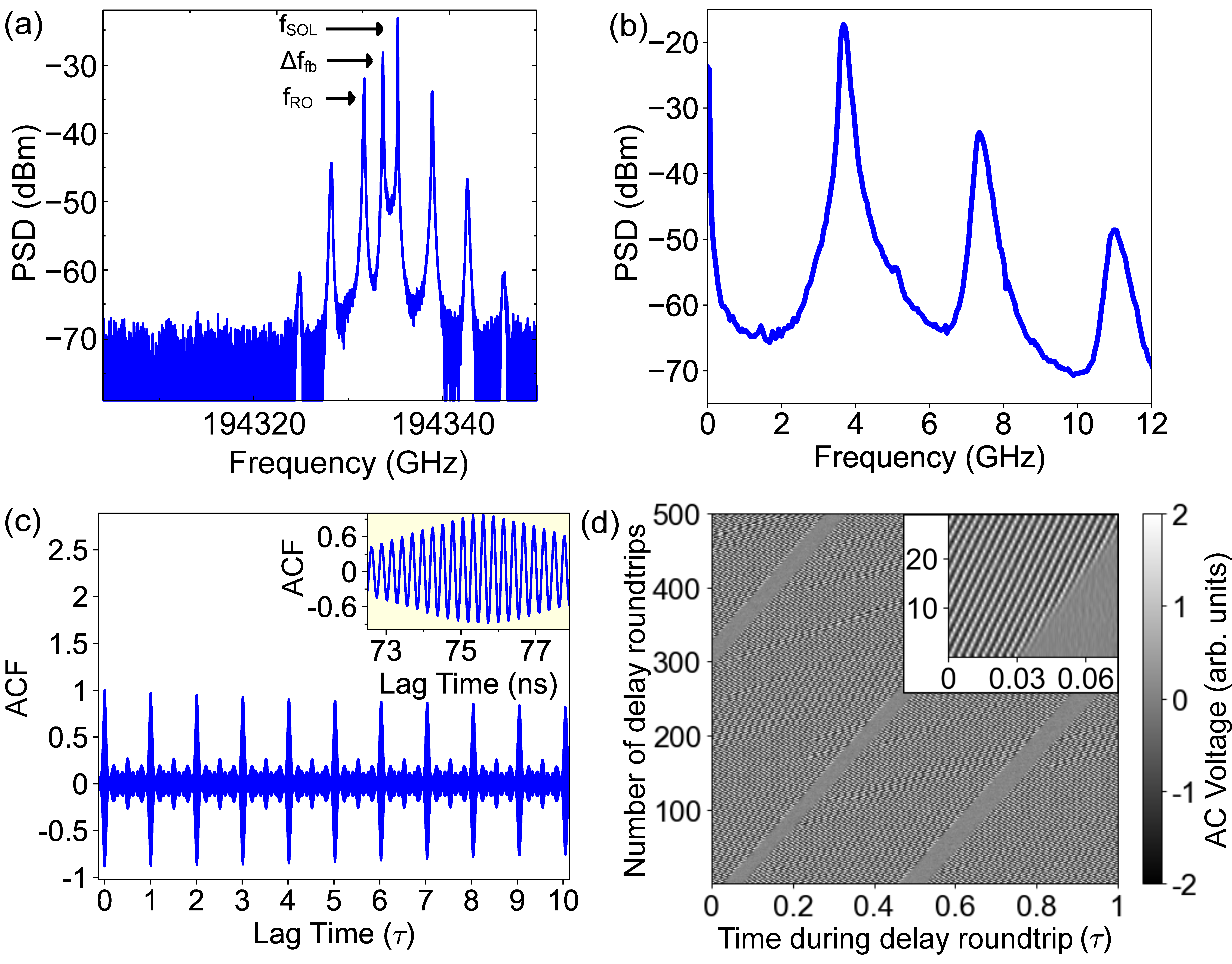
3.2. Intermediate Feedback Rate

Here, we show results for a bias current of I = 16 mA (≃$1.3{\mathrm{I}}_{\mathrm{th}}$) and a feedback rate that has been attenuated by 13 dB from its maximum value. These parameter choices correspond to the intermediate feedback condition $f_{RO}\approx \mathsf{\Delta }{f}_{fb}$.

The intermediate feedback region can be associated with a strong chaos regime in the weak–strong chaos paradigm for delayed systems [47,48]. In this regime, all correlations in dynamic and spectral signatures are strongly reduced as a result of the enhanced nonlinear mixing between $f_{RO}$ and $\mathsf{\Delta }{f}_{fb}$. This feature can be identified in Figure 8a, with a broad optical spectrum covering more than 20 GHz at −20 dB height. No sharp peaks are present neither in the optical spectrum nor in the RF power spectrum shown in Figure 8b.

The envelope of the ACF in Figure 8c illustrates the fast fading memory of the dynamics at successive delay echoes for these experimental conditions. The ACF height at the first delay echo is below 0.3, as visible in the inset. This low value of the ACF at multiples of $\tau$ is a signature of strong chaos in delayed feedback lasers [48]. Figure 8d depicts the spatio-temporal representation for such time series. The spatio-temporal plot shows differentiated structures with little correlation between them, disappearing rapidly and losing their correlation within a few delay times.

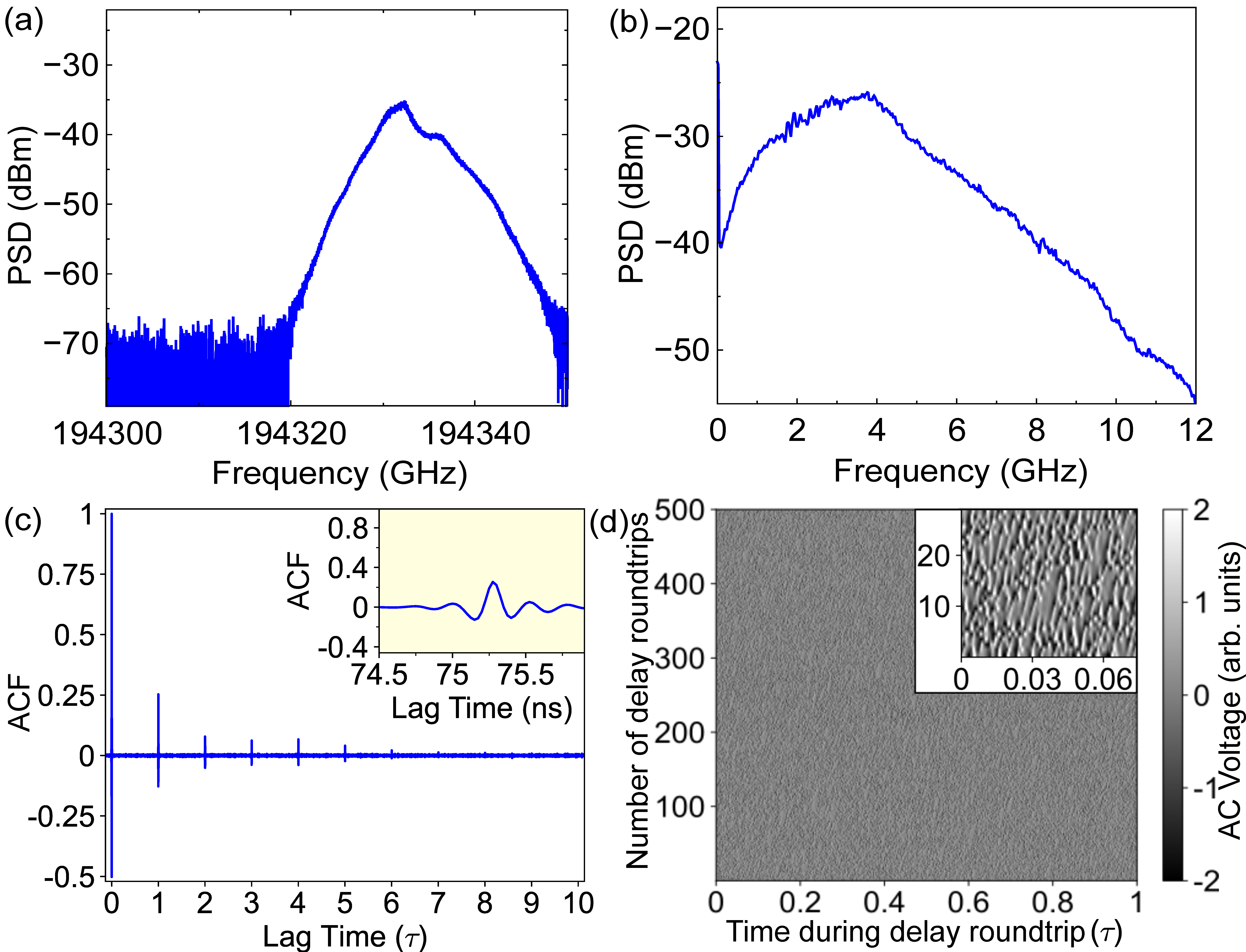
3.3. High Feedback Rate

Strong feedback conditions are depicted in Figure 9. In this case, the bias current is I = 13 mA (≃$1.1{\mathrm{I}}_{\mathrm{th}}$) and the feedback rate is the maximum value allowed in the experimental set-up, yielding the condition $f_{RO}<\mathsf{\Delta }{f}_{fb}$.

The optical spectrum in Figure 9a shows a two-peaked structure with a distance of ∼20 GHz between the peaks. The highest peak, at lower optical frequencies, corresponds to the spectral signature of the maximum feedback-induced frequency shift ($\mathsf{\Delta }{f}_{fb}$), while the peak at the right hand side of the spectrum is the signature of the dynamics in the region of the solitary laser mode. The RF power spectrum in Figure 9b illustrates that the chaotic bandwidth broadens when the feedback rate is increased, with the particularity that the power for low frequencies significantly increases (see inset of Figure 9b). This increase of the RF power density at lower frequencies is due to the appearance of the so-called low frequency fluctuations (LFF) in the intensity dynamics. The LFF dynamics, which appear for currents close to the lasing threshold and strong feedback, is characterized by irregularly distributed dropouts in the intensity dynamics [49,50,51]. The LFF power dropouts are distinguishable in Figure 9d as dark horizontal lines that typically last a $\tau$-interval and repeat irregularly every ∼$20\tau$. Here, LFFs are observed in the strong feedback case since the laser is operated close to the lasing threshold $\mathrm{I}\simeq 1.1{\mathrm{I}}_{\mathrm{th}}$.

The high feedback rate conditions lead to large delay-induced correlation peaks, as shown in detail at the inset in Figure 9c. Despite the fast chaotic dynamics and a broad RF spectrum, the slow decay of the ACF envelope hints at the fact that this dynamics correspond to a weak chaos regime [48]. The long-term vertical propagation of the structures visible in the spatio-temporal representation of Figure 9d (and magnified in the inset) supports this interpretation. In delayed feedback SL, strong chaos does not occur when feedback is strongest, but rather in the region where the feedback induced frequency shift approaches the frequency of the relaxation oscillations of the solitary laser [42]. It is worth noting that, when the feedback is strong enough, the laser again enters the weak chaos regime and, eventually, for particularly strong feedback and bias currents not far from threshold, the laser intensity can be stabilized again. This latter scenario leads the laser to a particularly high coherent state [31].

4. Discussion and Conclusions

The complex dynamical behavior of SL subject to optical feedback leaves characteristic fingerprints that can be observed in time and frequency domains. In this tutorial, we presented a basic overview of the main dynamical phenomena and the feedback-induced features in optical spectra and laser intensity measurements of single-mode SL. The impact of optical feedback on multi-mode lasers is a further, interesting aspect that has not been covered here. We have focused instead on the conditions where long delayed optical feedback yields a transition between stable dynamics and undamped relaxation oscillations, as well as in two conditions that lead to two chaotic regimes of different natures. In all these cases, the interplay between the relaxation oscillations frequency $f_{RO}$ and the maximum feedback-induced frequency shift $\mathsf{\Delta }{f}_{fb}$ is crucial for the dynamics that can be observed in the laser. The particularities of the dynamical features, such as the shape of the optical spectrum or the structures in the spatio-temporal representation, do, however, depend on the parameters of the considered device. In particular, lasers with a higher linewidth enhancement factor $\alpha$ are typically more sensitive to feedback.

By directly detecting the laser emission with a photodiode, one gets information about the intensity dynamics. Characterization of the phase dynamics is more challenging but also possible through, e.g., heterodyne measurements [52]. For the heterodyne technique, the field of the delayed-feedback laser is coherently added to the field of a narrow linewidth laser of a similar optical frequency, and the mixed fields are then detected by a fast photodetector. In this manner, a signal proportional to the optical frequency dynamics can be measured in the radio-frequency domain. By simultaneously measuring intensity and optical frequency dynamics, along with the carrier dynamics, with high temporal resolution, one obtains a complete picture of the dynamical evolution of the laser along the three dynamical dimensions of the corresponding rate equation model [53]. The full knowledge of the dynamics can allow for tailoring the response of the laser for applications by performing a proper phase space engineering.

In the last few years, the study of SL with optical feedback has been extended beyond the single, fixed delay case. From the fundamental point of view, two notable extensions include the realization of state-dependent delays [54] or 2D spatio-temporal dynamics [55] in laser systems with two delays. From the application point of view, SL subject to optical feedback and optical injection have been demonstrated to allow for information processing in the context of photonic reservoir computing [20,56]. We envision that the complex dynamics of SL with optical feedback described in this tutorial will still prove to be a valuable resource for further research and innovation.

References

1. Hall, R.; Fenner, G.; Kingsley, J.; Soltys, T.; Carlson, R. Coherent Light Emission From GaAs Junctions. Phys. Rev. Lett. 1962, 9, 366–368. [Google Scholar] [CrossRef]
2. Nathan, M.I.; Dumke, W.P.; Burns, G.; Dill, F.H.; Lasher, G. Stimulated Emission of Radiation from GaAs p-n Junctions. Appl. Phys. Lett. 1962, 1, 62. [Google Scholar] [CrossRef]
3. Quist, T.M.; Rediker, R.H.; Keyes, R.J.; Krag, W.E.; Lax, B.; McWhorter, A.L.; Zeigler, H.J. Semiconductor Maser of GaAs. Appl. Phys. Lett. 1962, 1, 91. [Google Scholar] [CrossRef]
4. Coleman, J.J. The development of the semiconductor laser diode after the first demonstration in 1962. Semicond. Sci. Technol. 2012, 27, 090207. [Google Scholar] [CrossRef]
5. Broom, R. Self modulation at gigahertz frequencies of a diode laser coupled to an external cavity. Electron. Lett. 1969, 5, 571. [Google Scholar] [CrossRef]
6. Broom, R.; Mohn, E.; Risch, C.; Salathe, R. Microwave self-modulation of a diode laser coupled to an external cavity. IEEE J. Quantum Electron. 1970, 6, 328–334. [Google Scholar] [CrossRef]
7. Risch, C.; Voumard, C. Self-pulsation in the output intensity and spectrum of GaAs-AlGaAs cw diode lasers coupled to a frequency-selective external optical cavity. J. Appl. Phys. 1977, 48, 2083. [Google Scholar] [CrossRef]
8. Lenstra, D.; Verbeek, B.; den Boef, A. Coherence collapse in single-mode semiconductor lasers due to optical feedback. IEEE J. Quantum Electron. 1985, 21, 674–679. [Google Scholar] [CrossRef]
9. Tkach, R.; Chraplyvy, A. Regimes of feedback effects in 1.5-um distributed feedback lasers. J. Light. Technol. 1986, 4, 1655–1661. [Google Scholar] [CrossRef]
10. Mørk, J.; Tromborg, B.; Mark, J. Chaos in semiconductor lasers with optical feedback: Theory and experiment. IEEE J. Quantum Electron. 1992, 28, 93–108. [Google Scholar] [CrossRef]
11. Heil, T.; Fischer, I.; Elsäßer, W. Stabilization of feedback-induced instabilities in semiconductor lasers. J. Opt. B Quantum Semiclassical Opt. 2000, 2, 413–420. [Google Scholar] [CrossRef] [Green Version]
12. Ahlers, V.; Parlitz, U.; Lauterborn, W. Hyperchaotic dynamics and synchronization of external-cavity semiconductor lasers. Phys. Rev. E 1998, 58, 7208. [Google Scholar] [CrossRef] [Green Version]
13. Vicente, R.; Daudén, J.; Colet, P.; Toral, R. Analysis and characterization of the hyperchaos generated by a semiconductor laser subject to a delayed feedback loop. IEEE J. Quantum Electron. 2005, 41, 541–548. [Google Scholar] [CrossRef] [Green Version]
14. Heil, T.; Fischer, I.; Elsässer, W.; Mulet, J.; Mirasso, C. Chaos Synchronization and Spontaneous Symmetry-Breaking in Symmetrically Delay-Coupled Semiconductor Lasers. Phys. Rev. Lett. 2001, 86, 795–798. [Google Scholar] [CrossRef] [PubMed] [Green Version]
15. Locquet, A.; Masoller, C.; Mirasso, C.R. Synchronization regimes of optical-feedback-induced chaos in unidirectionally coupled semiconductor lasers. Phys. Rev. E 2002, 65, 056205. [Google Scholar] [CrossRef] [PubMed] [Green Version]
16. Argyris, A.; Syvridis, D.; Larger, L.; Annovazzi-Lodi, V.; Colet, P.; Fischer, I.; García-Ojalvo, J.; Mirasso, C.R.; Pesquera, L.; Shore, K.A. Chaos-based communications at high bit rates using commercial fibre-optic links. Nature 2005, 438, 343–346. [Google Scholar] [CrossRef]
17. Uchida, A.; Amano, K.; Inoue, M.; Hirano, K.; Naito, S.; Someya, H.; Oowada, I.; Kurashige, T.; Shiki, M.; Yoshimori, S.; et al. Fast physical random bit generation with chaotic semiconductor lasers. Nat. Photonics 2008, 2, 728–732. [Google Scholar] [CrossRef]
18. Peil, M.; Fischer, I.; Elsäßer, W.; Bakić, S.; Damaschke, N.; Tropea, C.; Stry, S.; Sacher, J. Rainbow refractometry with a tailored incoherent semiconductor laser source. Appl. Phys. Lett. 2006, 89, 091106. [Google Scholar] [CrossRef] [Green Version]
19. Lin, F.-Y.; Liu, J.-M. Chaotic LIDAR. IEEE J. Sel. Top. Quantum Electron. 2004, 10, 991–997. [Google Scholar] [CrossRef]
20. Brunner, D.; Soriano, M.C.; Mirasso, C.R.; Fischer, I. Parallel photonic information processing at gigabyte per second data rates using transient states. Nat. Commun. 2013, 4, 1364. [Google Scholar] [CrossRef] [Green Version]
21. Pyragas, K. Continuous control of chaos by self-controlling feedback. Phys. Lett. A 1992, 170, 421–428. [Google Scholar] [CrossRef]
22. Stepan, G. Delay effects in brain dynamics. Introduction. Philos. Trans. Ser. Math. Phys. Eng. 2009, 367, 1059–1062. [Google Scholar]
23. Orosz, G.; Wilson, R.E.; Szalai, R.; Stépán, G. Exciting traffic jams: Nonlinear phenomena behind traffic jam formation on highways. Phys. Rev. E 2009, 80, 046205. [Google Scholar] [CrossRef] [PubMed]
24. Mackey, M.C.; Glass, L. Oscillation and chaos in physiological control systems. Science 1977, 197, 287–289. [Google Scholar] [CrossRef] [PubMed]
25. Elowitz, M.B.; Leibler, S. A synthetic oscillatory network of transcriptional regulators. Nature 2000, 403, 335–338. [Google Scholar] [CrossRef]
26. Chen, L.; Aihara, K. Stability of genetic regulatory networks with time delay. IEEE Trans. Circuits Syst. Fundam. Appl. 2002, 49, 602–608. [Google Scholar] [CrossRef]
27. Yeung, M.; Strogatz, S. Time Delay in the Kuramoto Model of Coupled Oscillators. Phys. Rev. Lett. 1999, 82, 648–651. [Google Scholar] [CrossRef] [Green Version]
28. Keuninckx, L.; Soriano, M.C.; Fischer, I.; Mirasso, C.R.; Nguimdo, R.M.; van der Sande, G. Encryption key distribution via chaos synchronization. Sci. Rep. 2017, 7, 43428. [Google Scholar] [CrossRef] [Green Version]
29. Soriano, M.C.; García-Ojalvo, J.; Mirasso, C.R.; Fischer, I. Complex photonics: Dynamics and applications of delay-coupled semiconductors lasers. Rev. Mod. Phys. 2013, 85, 421–470. [Google Scholar] [CrossRef] [Green Version]
30. Kelly, B.; Phelan, R.; Jones, D.; Herbert, C.; O’Carroll, J.; Rensing, M.; Wendelboe, J.; Watts, C.; Kaszubowska-Anandarajah, A.; Guignard, C.; et al. Discrete mode laser diodes with very narrow linewidth emission. Electron. Lett. 2007, 43, 1282. [Google Scholar] [CrossRef] [Green Version]
31. Brunner, D.; Luna, R.; Latorre, A.D.i.; Porte, X.; Fischer, I. Semiconductor laser linewidth reduction by six orders of magnitude via delayed optical feedback. Opt. Lett. 2017, 42, 163–166. [Google Scholar] [CrossRef]
32. Baili, G.; Alouini, M.; Malherbe, T.; Dolfi, D.; Sagnes, I.; Bretenaker, F. Direct observation of the class-B to class-A transition in the dynamical behavior of a semiconductor laser. Europhys. Lett. 2009, 87, 44005. [Google Scholar] [CrossRef] [Green Version]
33. Porte, X.; D’Huys, O.; Jüngling, T.; Brunner, D.; Soriano, M.C.; Fischer, I. Autocorrelation properties of chaotic delay dynamical systems: A study on semiconductor lasers. Phys. Rev. E 2014, 90, 052911. [Google Scholar] [CrossRef] [Green Version]
34. Henry, C. Theory of the linewidth of semiconductor lasers. IEEE J. Quantum Electron. 1982, 18, 259–264. [Google Scholar] [CrossRef]
35. Fischer, I.; van Tartwijk, G.; Levine, A.; Elsässer, W.; Göbel, E.; Lenstra, D. Fast Pulsing and Chaotic Itinerancy with a Drift in the Coherence Collapse of Semiconductor Lasers. Phys. Rev. Lett. 1996, 76, 220–223. [Google Scholar] [CrossRef] [PubMed] [Green Version]
36. Arecchi, F.; Giacomelli, G.; Lapucci, A.; Meucci, R. Two-dimensional representation of a delayed dynamical system. Phys. Rev. A 1992, 45, R4225–R4228. [Google Scholar] [CrossRef]
37. Masoller, C. Spatiotemporal dynamics in the coherence collapsed regime of semiconductor lasers with optical feedback. Chaos 1997, 7, 455–462. [Google Scholar] [CrossRef] [PubMed]
38. Lang, R.; Kobayashi, K. External optical feedback effects on semiconductor injection laser properties. IEEE J. Quantum Electron. 1980, 16, 347–355. [Google Scholar] [CrossRef]
39. Petermann, K. External optical feedback phenomena in semiconductor lasers. IEEE J. Sel. Top. Quantum Electron. 1995, 1, 480–489. [Google Scholar] [CrossRef]
40. Sano, T. Antimode dynamics and chaotic itinerancy in the coherence collapse of semiconductor lasers with optical feedback. Phys. Rev. A 1994, 50, 2719–2726. [Google Scholar] [CrossRef] [PubMed]
41. Henry, C.; Kazarinov, R. Instability of semiconductor lasers due to optical feedback from distant reflectors. IEEE J. Quantum Electron. 1986, 22, 294–301. [Google Scholar] [CrossRef]
42. Porte, X.; Soriano, M.C.; Fischer, I. Similarity properties in the dynamics of delayed-feedback semiconductor lasers. Phys. Rev. A 2014, 89, 023822. [Google Scholar] [CrossRef] [Green Version]
43. Kim, B.; Li, N.; Locquet, A.; Citrin, D.S. Experimental bifurcation-cascade diagram of an external-cavity semiconductor laser. Opt. Express 2014, 22, 2348–2357. [Google Scholar] [CrossRef]
44. Mørk, J.; Mark, J.; Tromborg, B. Route to chaos and competition between relaxation oscillations for a semiconductor laser with optical feedback. Phys. Rev. Lett. 1990, 65, 1999–2002. [Google Scholar] [CrossRef] [PubMed]
45. Masoller, C.; Abraham, N.B. Stability and dynamical properties of the coexisting attractors of an external-cavity semiconductor laser. Phys. Rev. A 1998, 57, 1313–1322. [Google Scholar] [CrossRef] [Green Version]
46. Dong, J.X.; Ruan, J.; Zhang, L.; Zhuang, J.P.; Chan, S.C. Stable-unstable switching dynamics in semiconductor lasers with external cavities. Phys. Rev. A 2021, 103, 053524. [Google Scholar] [CrossRef]
47. Heiligenthal, S.; Dahms, T.; Yanchuk, S.; Jüngling, T.; Flunkert, V.; Kanter, I.; Schöll, E.; Kinzel, W. Strong and Weak Chaos in Nonlinear Networks with Time-Delayed Couplings. Phys. Rev. Lett. 2011, 107, 234102. [Google Scholar] [CrossRef]
48. Heiligenthal, S.; Jüngling, T.; D’Huys, O.; Arroyo-Almanza, D.A.; Soriano, M.C.; Fischer, I.; Kanter, I.; Kinzel, W. Strong and weak chaos in networks of semiconductor lasers with time-delayed couplings. Phys. Rev. E 2013, 88, 012902. [Google Scholar] [CrossRef] [Green Version]
49. Mørk, J.; Tromborg, B.; Christiansen, P.L. Bistability and low-frequency fluctuations in semiconductor lasers with optical feedback: A theoretical analysis. IEEE J. Quantum Electron. 1988, 24, 123–133. [Google Scholar] [CrossRef] [Green Version]
50. Sukow, D.W.; Gardner, J.R.; Gauthier, D.J. Statistics of power-dropout events in semiconductor lasers with time-delayed optical feedback. Phys. Rev. A 1997, 56, R3370. [Google Scholar] [CrossRef]
51. Heil, T.; Fischer, I.; Elsäßer, W. Coexistence of low-frequency fluctuations and stable emission on a single high-gain mode in semiconductor lasers with external optical feedback. Phys. Rev. A 1998, 58, R2672–R2675. [Google Scholar] [CrossRef] [Green Version]
52. Brunner, D.; Porte, X.; Soriano, M.C.; Fischer, I. Real-time frequency dynamics and high-resolution spectra of a semiconductor laser with delayed feedback. Sci. Rep. 2012, 2, 732. [Google Scholar] [CrossRef] [Green Version]
53. Brunner, D.; Soriano, M.C.; Porte, X.; Fischer, I. Experimental Phase-Space Tomography of Semiconductor Laser Dynamics. Phys. Rev. Lett. 2015, 115, 053901. [Google Scholar] [CrossRef] [PubMed] [Green Version]
54. Martínez-Llinàs, J.; Porte, X.; Soriano, M.C.; Colet, P.; Fischer, I. Dynamical properties induced by state-dependent delays in photonic systems. Nat. Commun. 2015, 6, 7425. [Google Scholar] [CrossRef] [PubMed] [Green Version]
55. Yanchuk, S.; Giacomelli, G. Pattern formation in systems with multiple delayed feedbacks. Phys. Rev. Lett. 2014, 112, 174103. [Google Scholar] [CrossRef] [Green Version]
56. Van der Sande, G.; Brunner, D.; Soriano, M.C. Advances in photonic reservoir computing. Nanophotonics 2017, 6, 561–576. [Google Scholar] [CrossRef]
Figure 1. Scheme of our typical experimental setup to study feedback dynamics. LD: laser diode, Circ: optical circulator, PC: polarization controller; Att: optical attenuator, Spl: one by two intensity splitter with R = 0.95 and (1 − R ) = 0.05 splitting ratios, →: optical isolator, and PD: photodiode.
Photonics 09 00047 g001
Figure 2. Power-current characteristics of a single-mode laser under different operation conditions: in solitary emission (blue line) and when subject to delayed optical feedback (orange line). The inset is a magnification of the region around the two distinct laser thresholds.
Photonics 09 00047 g002
Figure 3. Experimental signatures of delayed optical feedback on the optical and radio-frequency (RF) spectra of a semiconductor laser. (a) High-resolution optical spectra of the laser without feedback (orange) and with different amounts of feedback. (b) Effect of delayed optical feedback on the RF power spectral density. The RF spectrum is depicted over a 15 GHz frequency span for increasing feedback conditions. RF spectra are shown for the solitary laser emission (orange line) and four successively higher values of the feedback rate (from red towards blue). Inset: Zoom of the first 100 MHz for the maximum feedback rate. The external cavity frequency resonances are here clearly visible as equidistant peaks separated by 13.29 MHz. The arrow indicates the broadening direction of the optical spectrum and the overall bandwidth increase of the RF spectrum when the feedback rate increases, respectively.
Photonics 09 00047 g003
Figure 4. Fingerprint of the coherence collapse phenomenon on the intensity dynamics. The AC-coupled (average power is subtracted by a photodiode, with a low cut-off frequency of a few kHz) time traces are plotted in (a) for the solitary laser and (b) for the laser subject to delayed feedback. Colors correspond to the experimental conditions depicted in blue and orange colors in Figure 3. In (b), the tens of GHz laser’s optical linewidth is reflected in fast and chaotic oscillations of the corresponding time trace.
Photonics 09 00047 g004
Figure 5. Different representations of the chaotic intensity dynamics of delayed feedback lasers. (a) The autocorrelation function (ACF) corresponding to the same feedback conditions as depicted in the intensity dynamics of Figure 4b. The ACF was calculated over a time series of 2 million samples recorded with a sampling rate of 40 GS/s. (b) The spatio-temporal representation of the same chaotic time series. The abscissa denotes the time offset in a delay interval of length τ , while the vertical axis stacks the time series segments of length τ . The magnitude of the intensity fluctuations is color-coded.
Photonics 09 00047 g005
Figure 6. Ellipse of steady-state solutions for the Lang–Kobayashi model. External cavity modes are depicted as blue circles and antimodes as orange triangles. (a) Parameters: κ = 20 ns 1 , τ = 1 ns , and α = 2 . (b) Parameters: κ = 20 ns 1 , τ = 2 ns , and α = 2 . (c) Parameters: κ = 20 ns 1 , τ = 1 ns , and α = 4 .
Photonics 09 00047 g006
Figure 7. Characteristics for undamped relaxation oscillation dynamics at a bias current of I = 18 mA and a feedback rate that has been attenuated by 31 dB from its maximum value. (a) Optical spectrum, (b) RF power spectrum, (c) Autocorrelation function (ACF) of the intensity time series with inset around the first delay echo, (d) Spatio-temporal representation of the intensity time series with inset for magnification of the intensity dynamics around the origin.
Photonics 09 00047 g007
Figure 8. Exemplary dynamics at intermediate feedback levels. The bias current is I = 16 mA and the feedback rate has been attenuated by 13 dB from its maximum value. (a) Optical spectrum; (b) RF power spectrum; (c) Autocorrelation function (ACF) of the intensity time series with inset around the first delay echo, (d) Spatio-temporal representation of the intensity time series with inset for magnification around the origin.
Photonics 09 00047 g008
Figure 9. High feedback rate dynamics. The bias current is I = 13 mA and the feedback rate is the maximum value allowed in the experimental set-up. (a) Optical spectrum, (b) RF power spectrum, (c) Autocorrelation function (ACF) of the intensity time series with inset around the first delay echo, (d) Spatio-temporal representation of the intensity time series with inset for magnification around the origin.
Photonics 09 00047 g009
Publisher’s Note: MDPI stays neutral with regard to jurisdictional claims in published maps and institutional affiliations.