
From Data to Draught: Modelling and Predicting Mixed-Culture Beer Fermentation Dynamics Using Autoregressive Recurrent Neural Networks


Abstract
:1. Introduction
2. Materials and Methods
2.1. Materials
2.2. Methods
3. Results and Discussion
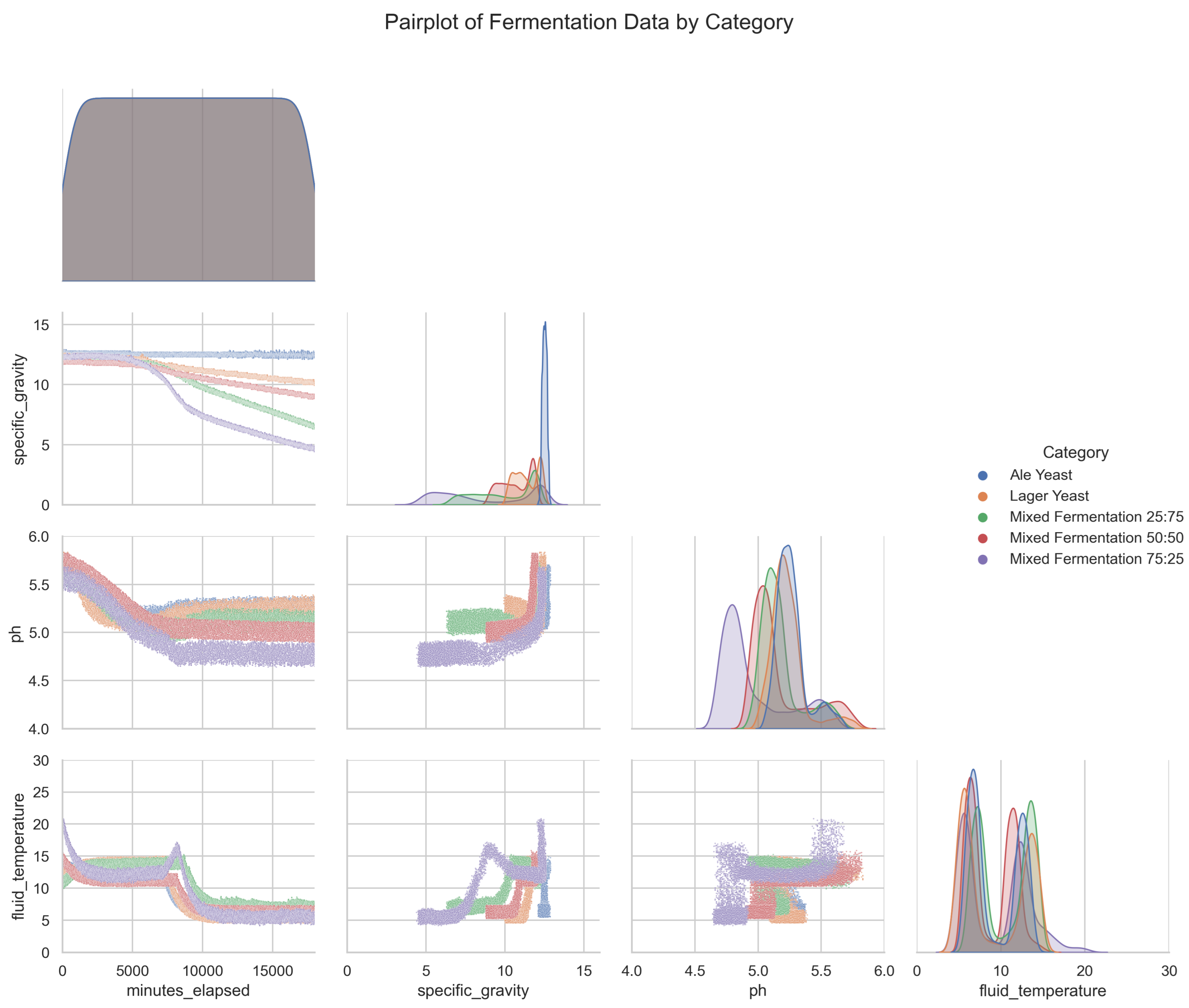
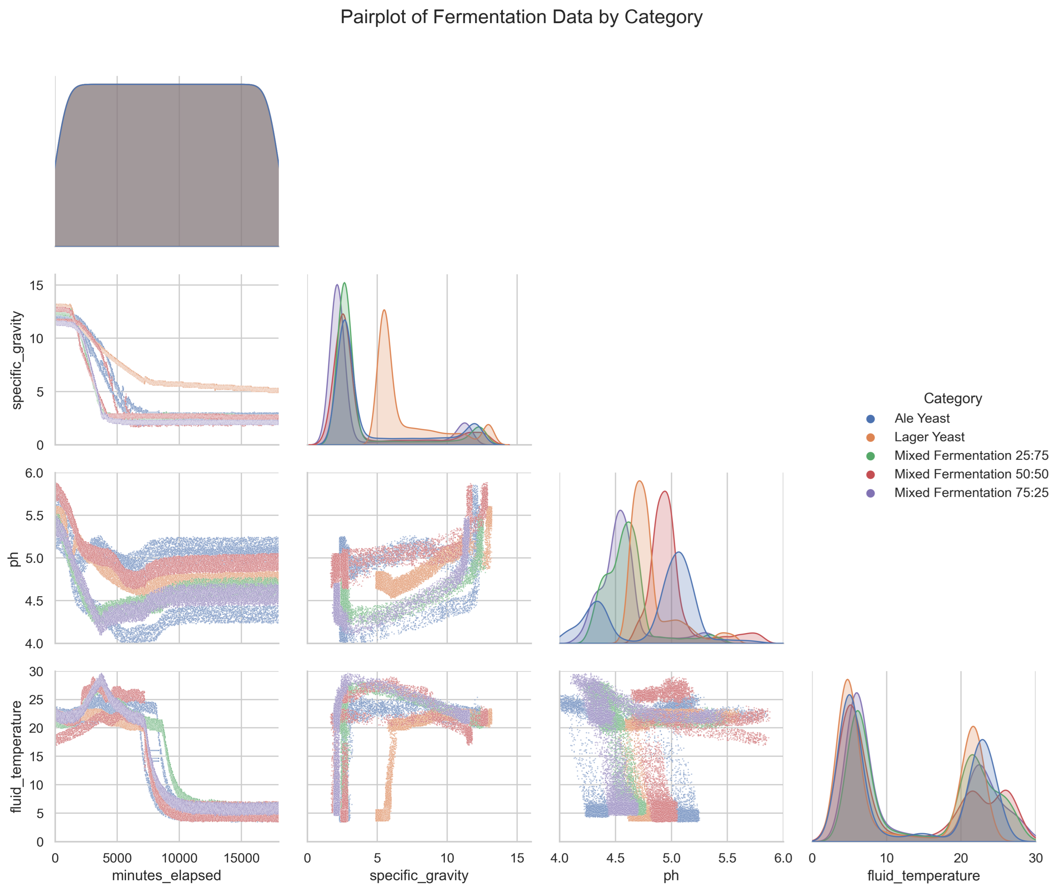
3.1. Training Data Characteristics
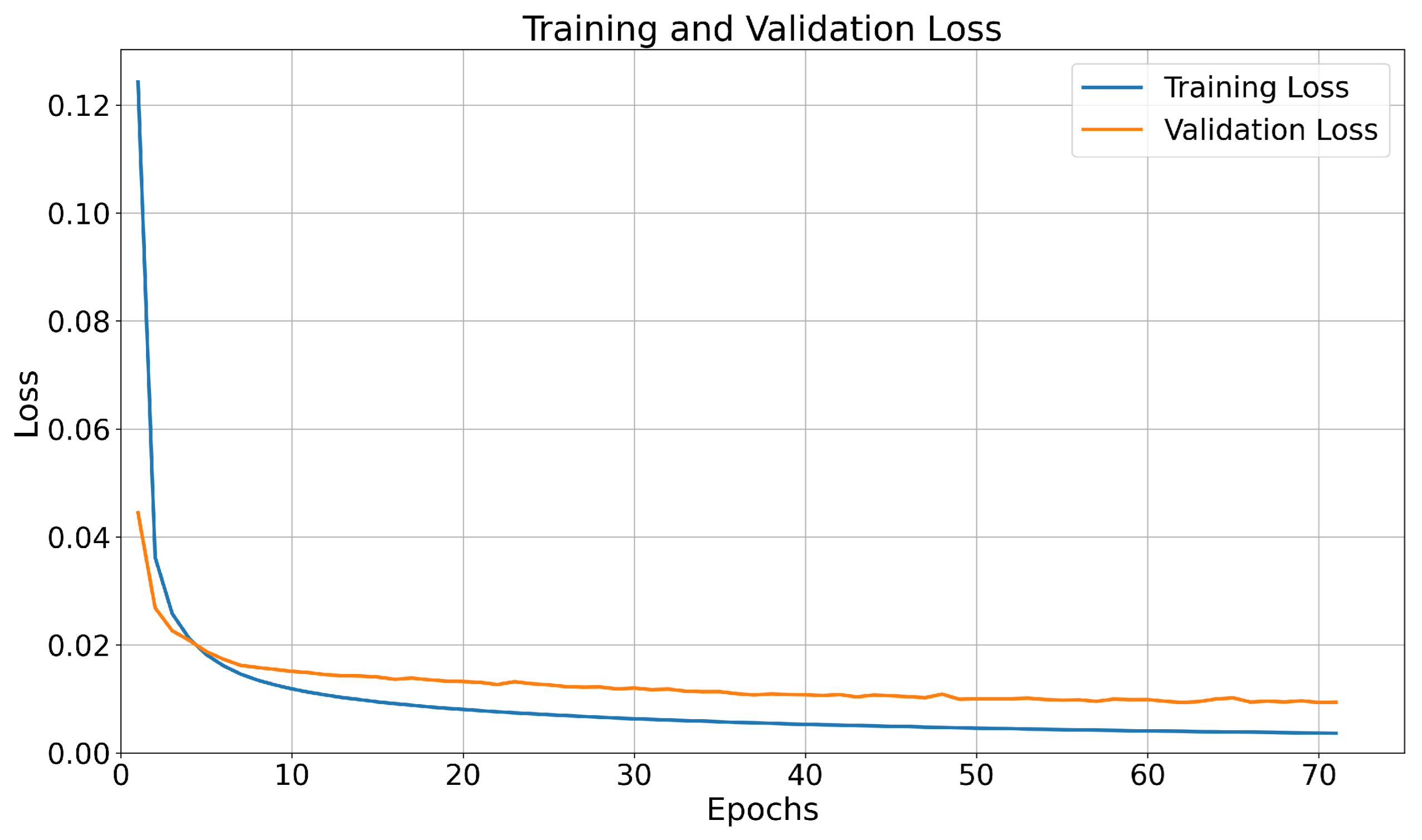
3.2. Hyperparameter Tuning
3.3. Residual Results for the AR-RNN Model
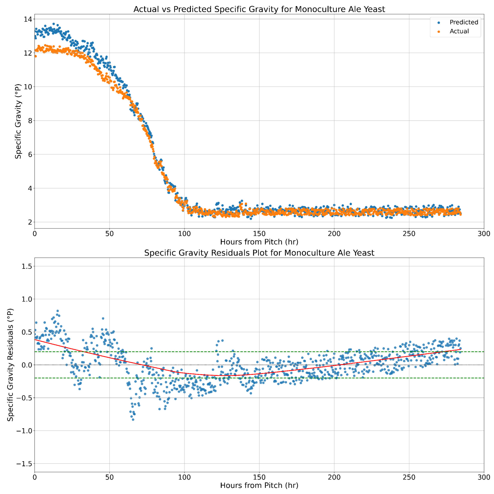
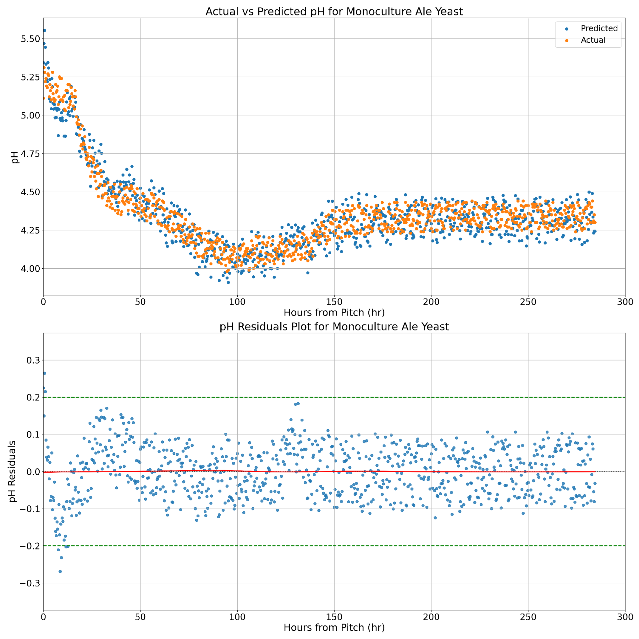
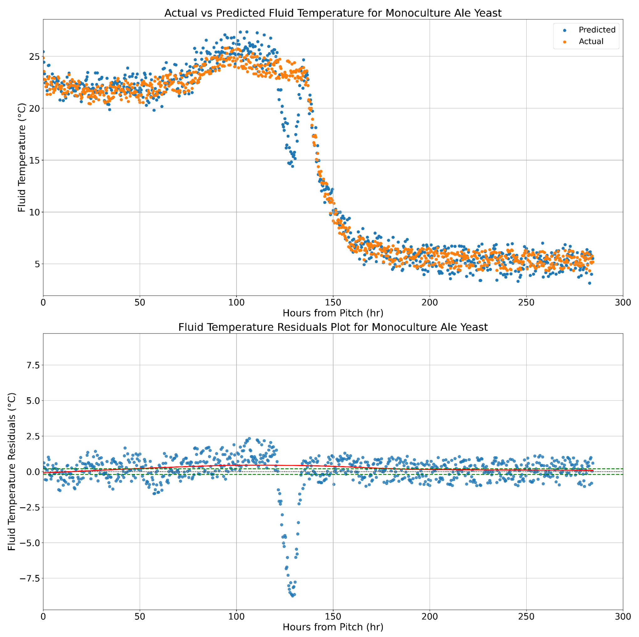
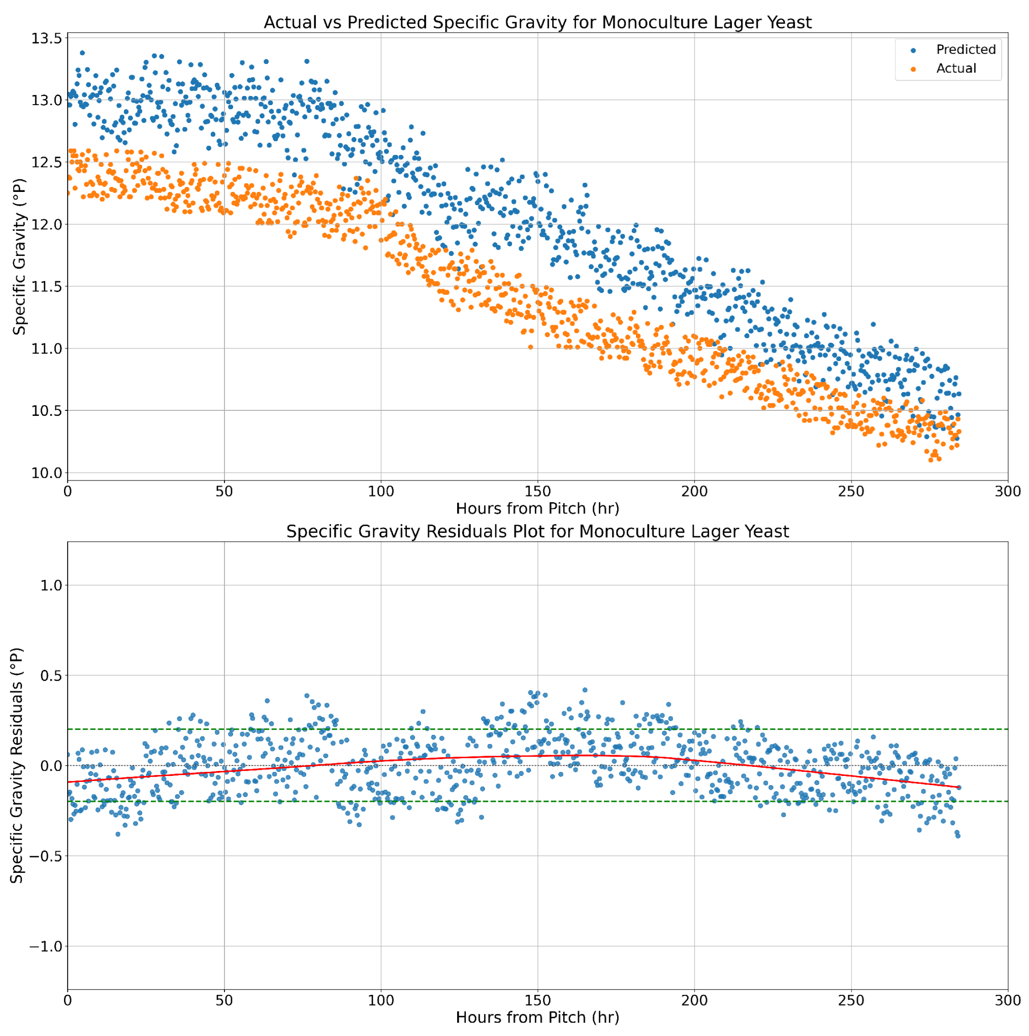
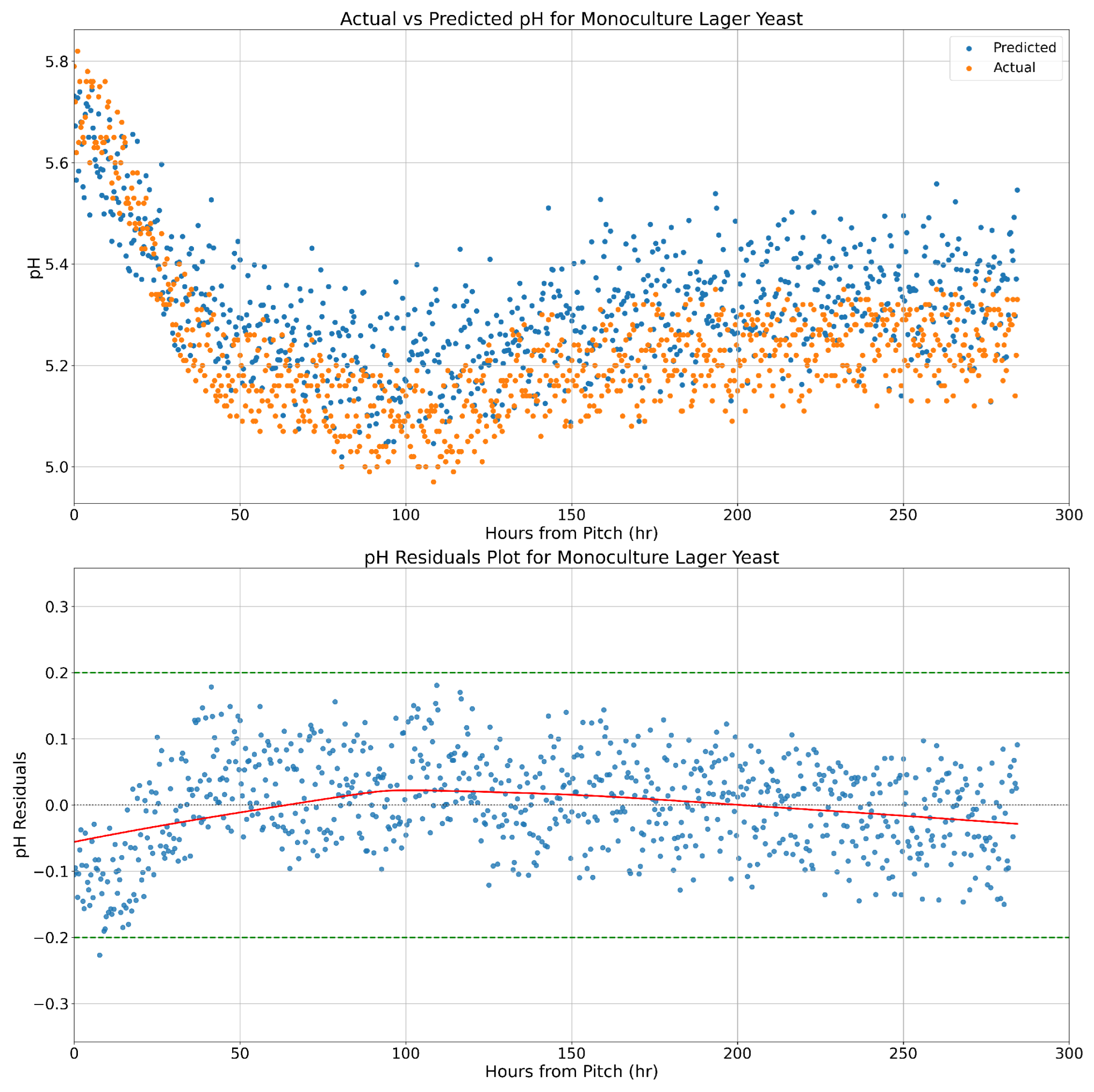
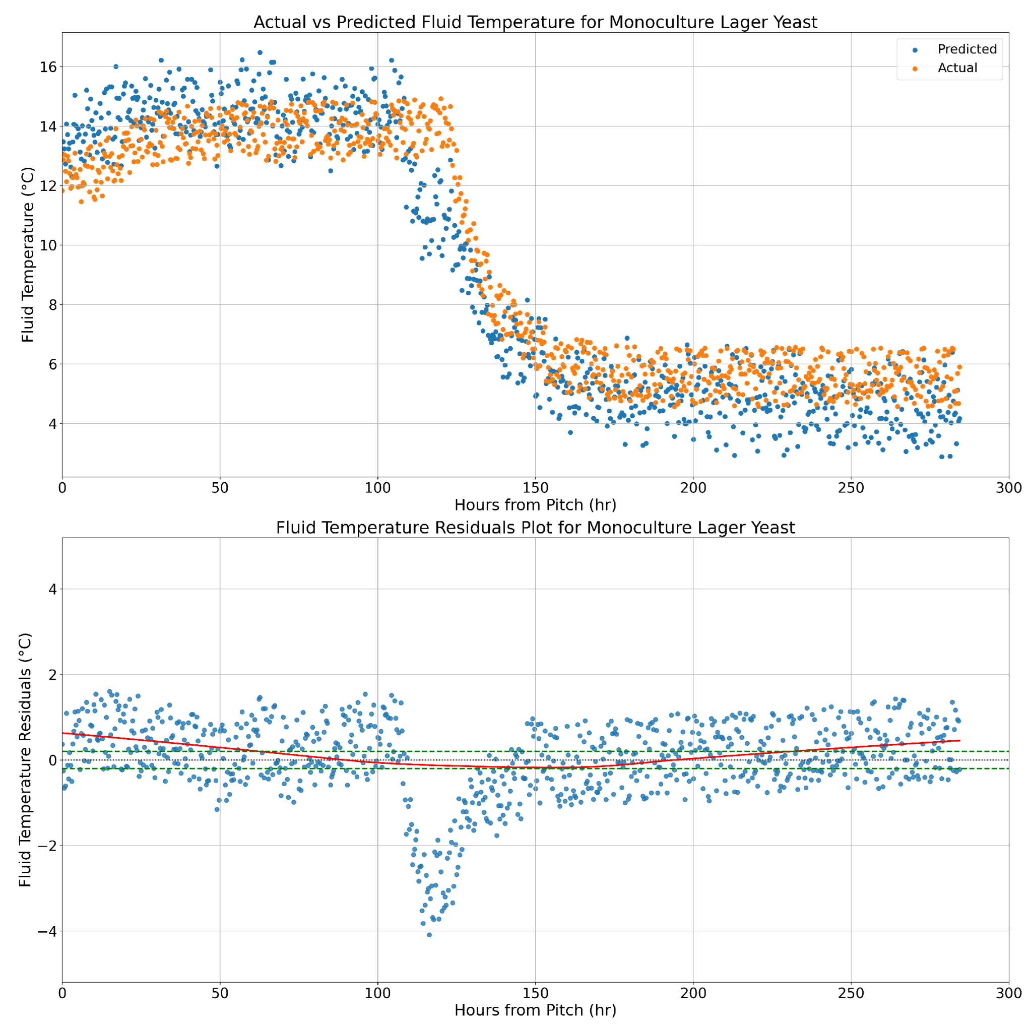
3.3.1. Monoculture Residuals
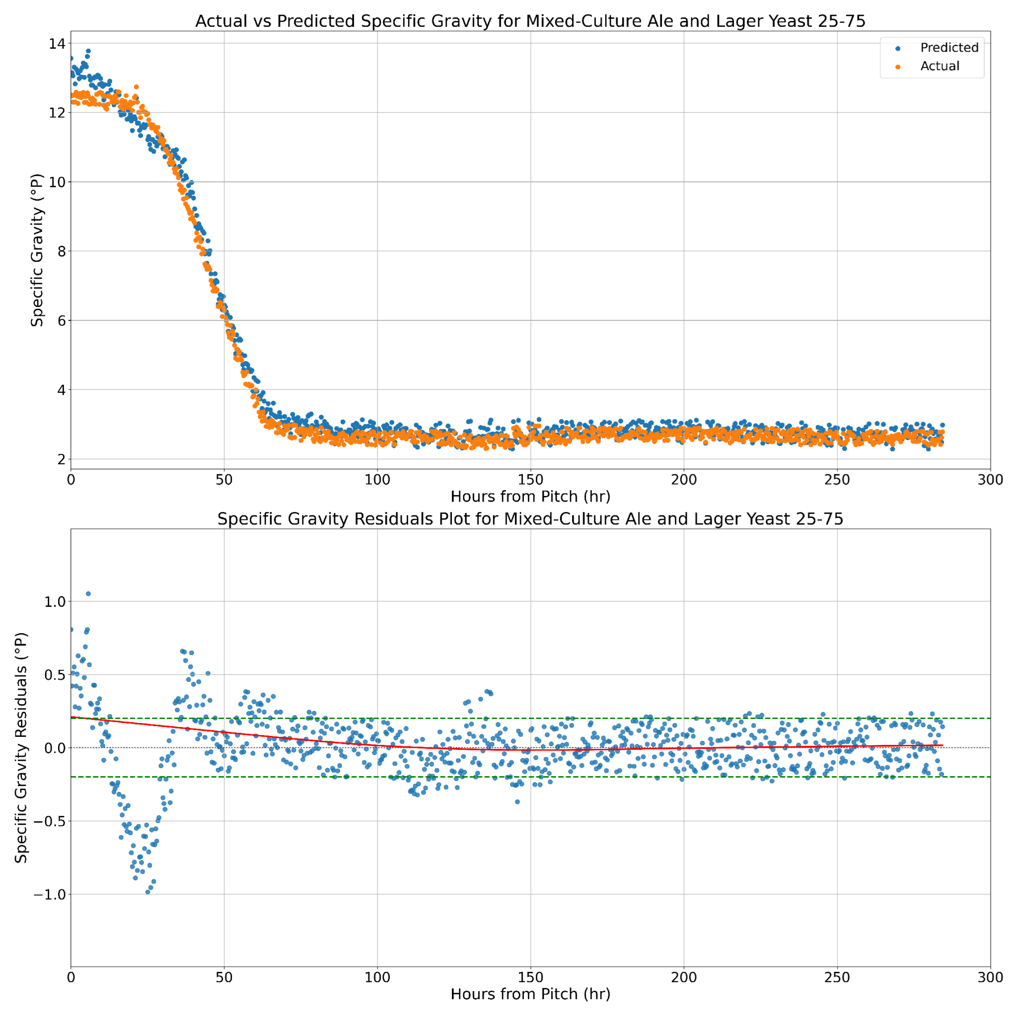
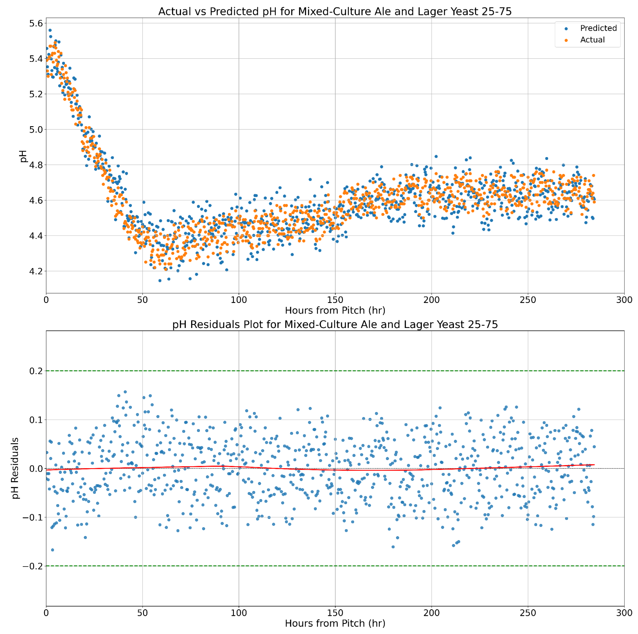
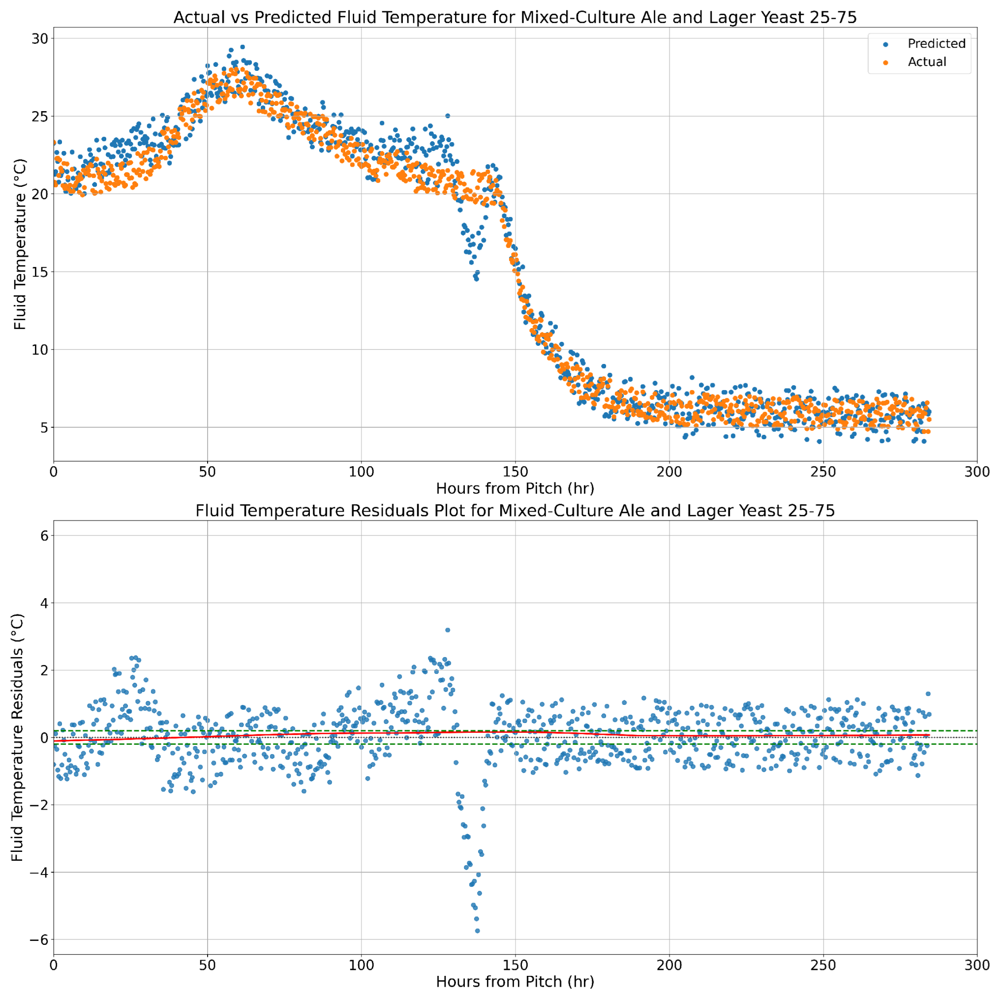
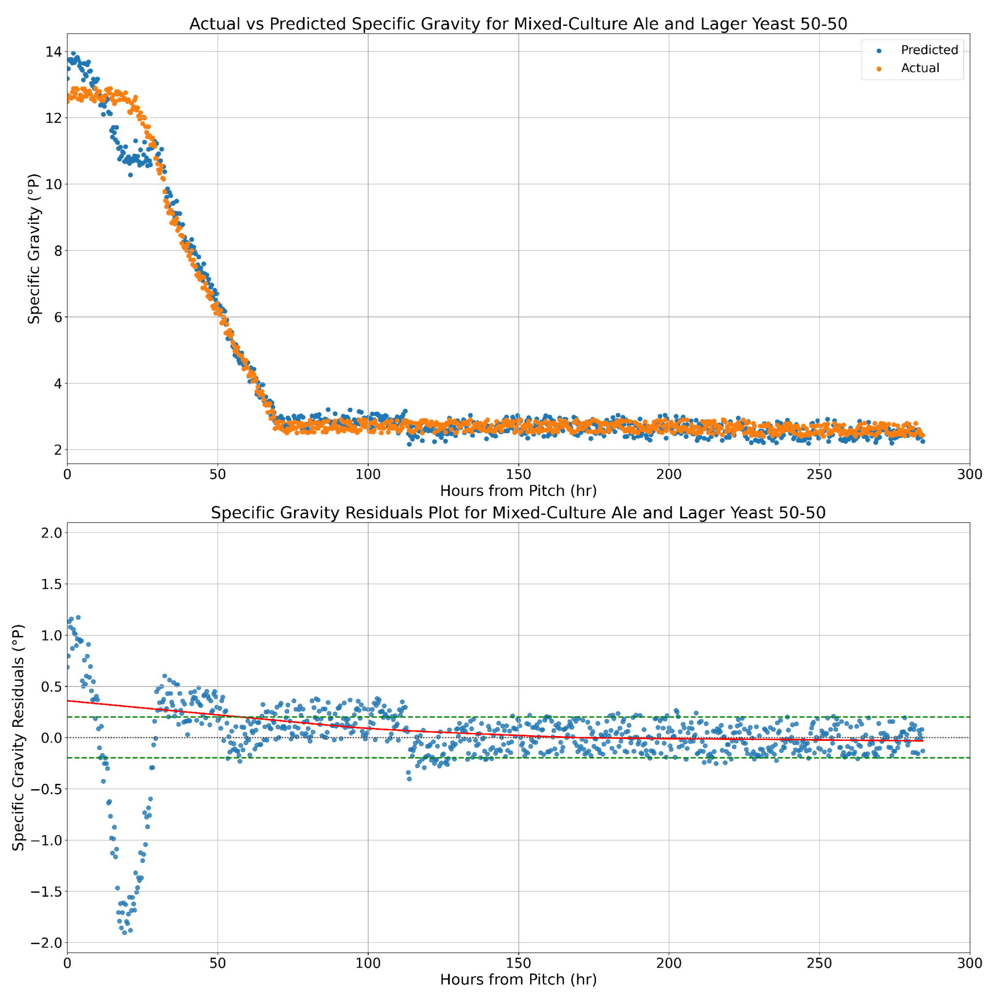
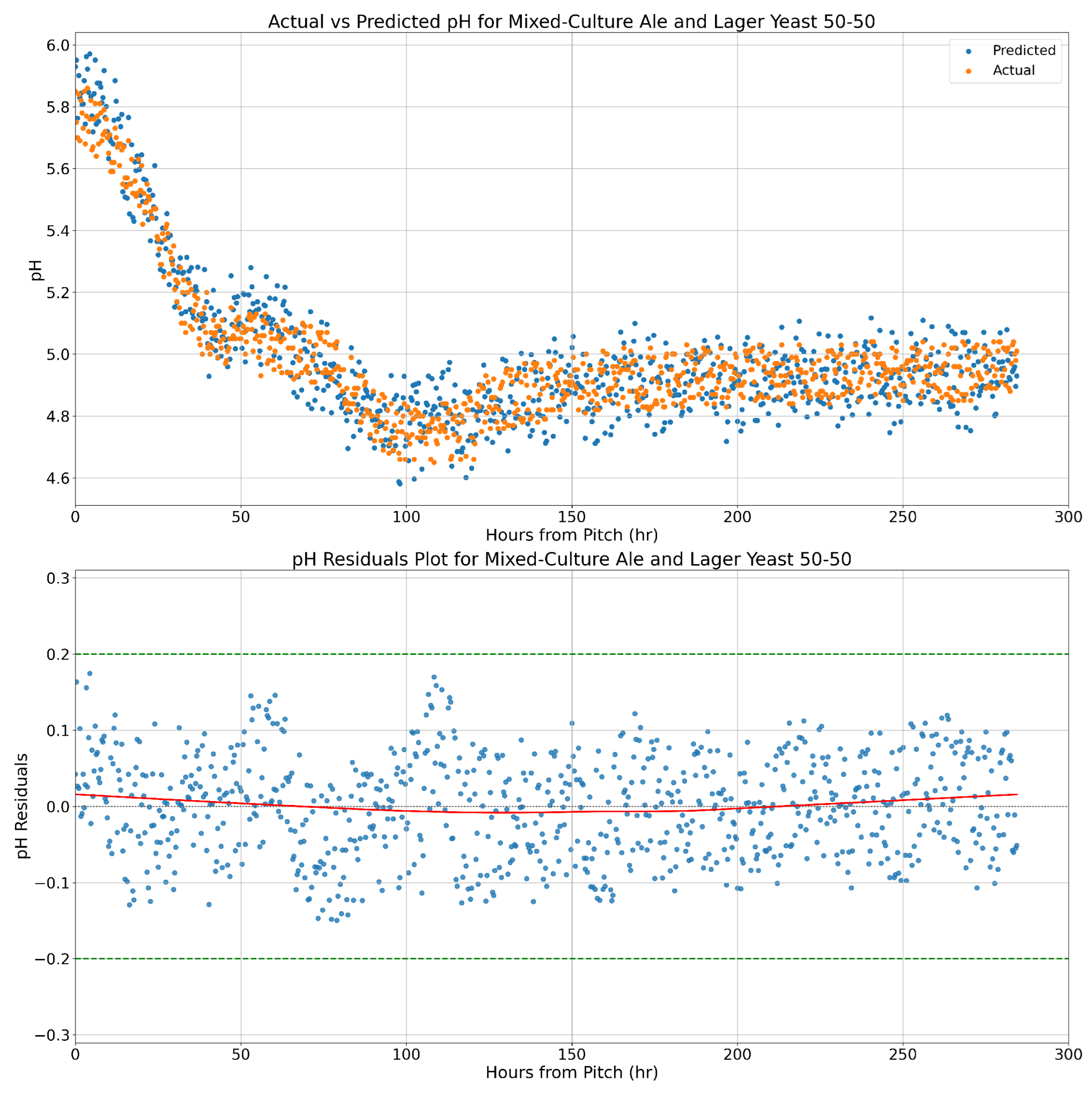
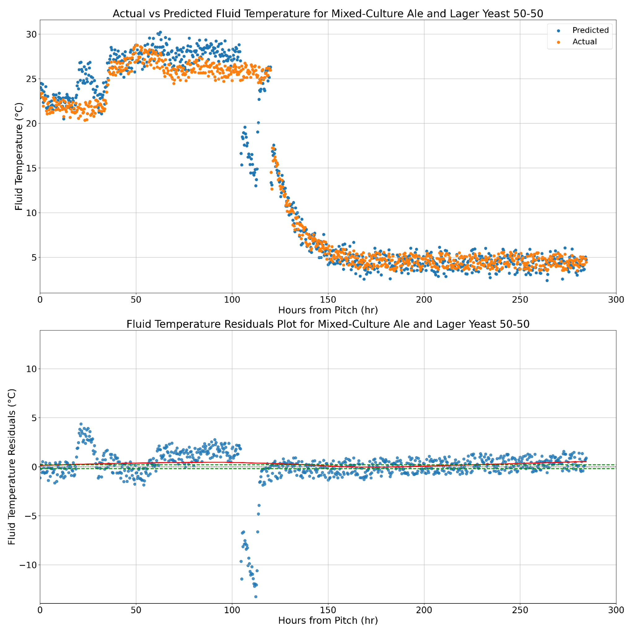
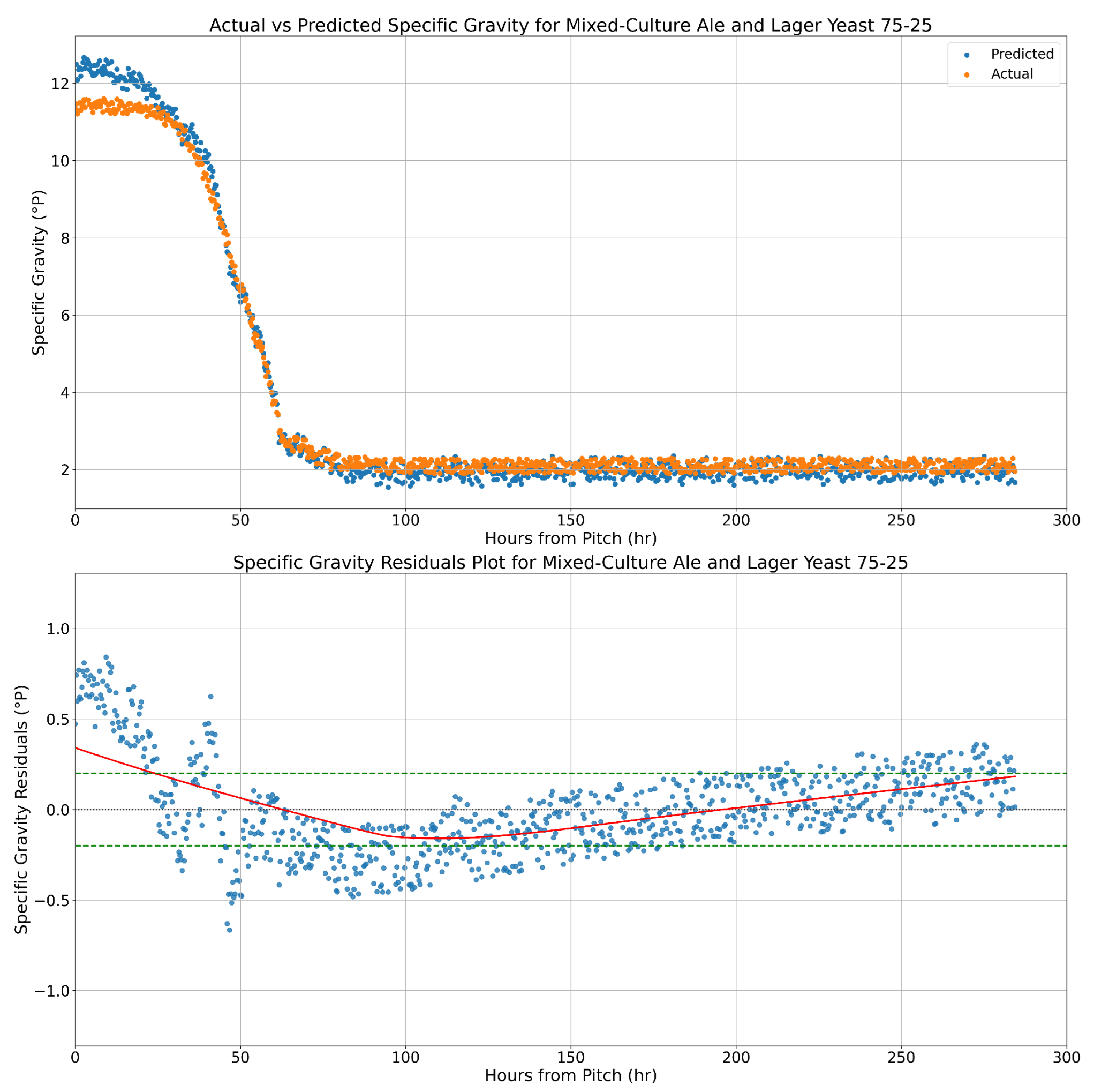
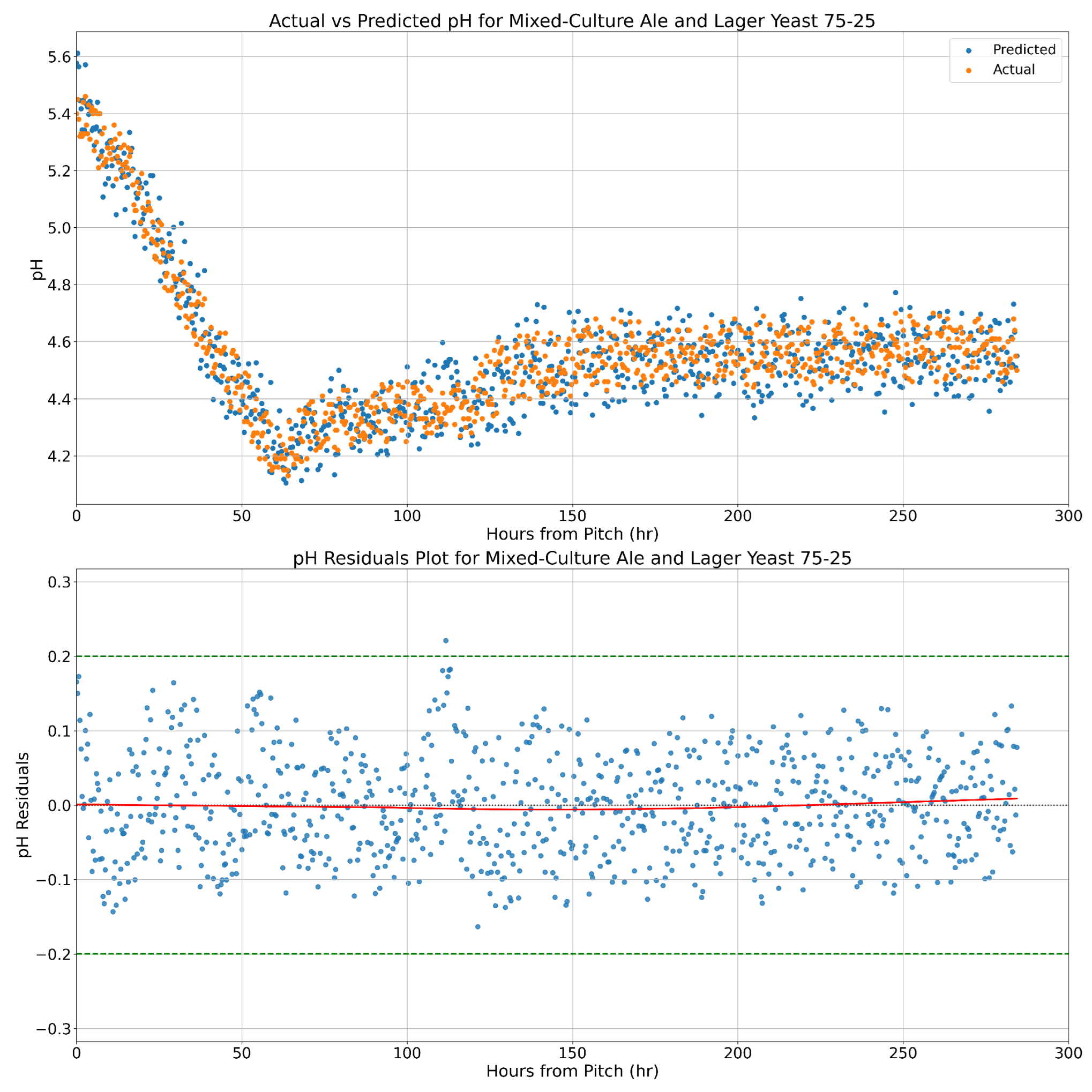
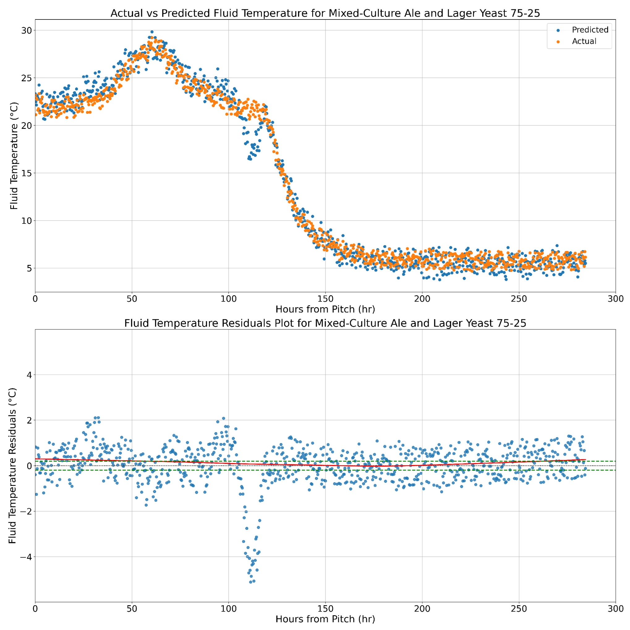
3.3.2. Mixed-Culture Residuals
3.4. Discussion
4. Conclusions
Author Contributions
Funding
Informed Consent Statement
Data Availability Statement
Conflicts of Interest
Abbreviations
| ANN | Artificial Neural Network |
| AR-RNN | Autoregressive Recurrent Neural Network |
| IoT | Internet of Things |
| LSTM | Long Short Term Memory |
| RNN | Recurrent Neural Network |
References
- Basso, R.F.; Alcarde, A.R.; Portugal, C.B. Could non-Saccharomyces yeasts contribute on innovative brewing fermentations? Food Res. Int. 2016, 86, 112–120. [Google Scholar] [CrossRef]
- Spitaels, F.; Wieme, A.D.; Janssens, M.; Aerts, M.; Van Landschoot, A.; De Vuyst, L.; Vandamme, P. The microbial diversity of an industrially produced lambic beer shares members of a traditionally produced one and reveals a core microbiota for lambic beer fermentation. Food Microbiol. 2015, 49, 23–32. [Google Scholar] [CrossRef] [PubMed]
- Van Oevelen, D.; Spaepen, M.; Timmermans, P.; Verachtert, H. Microbiological Aspects of Spontaneous Wort Fermentation in the Production of Lambic and Gueuze. J. Inst. Brew. 1977, 83, 356–360. [Google Scholar] [CrossRef]
- Sparrow, J. Wild Brews: Beer Beyond the Influence of Brewer’s Yeast; Brewers Publications: Kent, OH, USA, 2005. [Google Scholar]
- Tonsmeire, M. American Sour Beer: Innovative Techniques for Mixed Fermentations; Brewers Publications: Kent, OH, USA, 2014. [Google Scholar]
- Shimotsu, S.; Asano, S.; Iijima, K.; Suzuki, K.; Yamagishi, H.; Aizawa, M. Investigation of beer-spoilage ability of Dekkera/Brettanomyces yeasts and development of multiplex PCR method for beer-spoilage yeasts. J. Inst. Brew. 2015, 121, 177–180. [Google Scholar] [CrossRef]
- Serra Colomer, M.; Funch, B.; Forster, J. The raise of Brettanomyces yeast species for beer production. Curr. Opin. Biotechnol. 2019, 56, 30–35. [Google Scholar] [CrossRef]
- De Roos, J.; De Vuyst, L. Microbial acidification, alcoholization, and aroma production during spontaneous lambic beer production. J. Sci. Food Agric. 2019, 99, 25–38. [Google Scholar] [CrossRef]
- Dysvik, A.; La Rosa, S.L.; De Rouck, G.; Rukke, E.O.; Westereng, B.; Wicklund, T. Microbial Dynamics in Traditional and Modern Sour Beer Production. Appl. Environ. Microbiol. 2020, 86, e00566-20. [Google Scholar] [CrossRef]
- Martens, H.; Iserentant, D.; Verachtert, H. Microbiological Aspects of a Mixed Yeast—Bacterial Fermentation in the Production of a Special Belgian Acidic Ale. J. Inst. Brew. 1997, 103, 85–91. [Google Scholar] [CrossRef]
- White, C.; Zainasheff, J. Yeast: The Practical Guide to Beer Fermentation; Brewers Publications: Kent, OH, USA, 2010. [Google Scholar]
- Lodolo, E.J.; Kock, J.L.; Axcell, B.C.; Brooks, M. The yeast Saccharomyces Cerevisiae – Main Character Beer Brewing. FEMS Yeast Res. 2008, 8, 1018–1036. [Google Scholar] [CrossRef]
- de Andrés-Toro, B.; Girón-Sierra, J.M.; López-Orozco, J.A.; Fernández-Conde, C. Optimization of a Batch Fermentation Process by Genetic Algorithms. IFAC Proc. Vol. 1997, 30, 179–184. [Google Scholar] [CrossRef]
- de Andrés-Toro, B.; Girón-Sierra, J.; López-Orozco, J.; Fernández-Conde, C.; Peinado, J.; García-Ochoa, F. A kinetic model for beer production under industrial operational conditions. Math. Comput. Simul. 1998, 48, 65–74. [Google Scholar] [CrossRef]
- Toh, D.W.K.; Chua, J.Y.; Liu, S.Q. Impact of simultaneous fermentation with Saccharomyces cerevisiae and Torulaspora delbrueckii on volatile and non-volatile constituents in beer. LWT 2018, 91, 26–33. [Google Scholar] [CrossRef]
- Dysvik, A.; La Rosa, S.L.; Liland, K.H.; Myhrer, K.S.; Østlie, H.M.; De Rouck, G.; Rukke, E.O.; Westereng, B.; Wicklund, T. Co-fermentation Involving Saccharomyces cerevisiae and Lactobacillus Species Tolerant to Brewing-Related Stress Factors for Controlled and Rapid Production of Sour Beer. Front. Microbiol. 2020, 11, 279. [Google Scholar] [CrossRef]
- Bhonsale, S.; Mores, W.; Van Impe, J. Dynamic Optimisation of Beer Fermentation under Parametric Uncertainty. Fermentation 2021, 7, 285. [Google Scholar] [CrossRef]
- Hepworth, N.; Brown, A.K.; Hammond, J.R.M.; Boyd, J.W.R.; Varley, J. The Use of Laboratory-Scale Fermentations as a Tool for Modelling Beer Fermentations. Food Bioprod. Process. 2003, 81, 50–56. [Google Scholar] [CrossRef]
- Peleg, M. A New Look at Models of the Combined Effect of Temperature, pH, Water Activity, or Other Factors on Microbial Growth Rate. Food Eng. Rev. 2022, 14, 31–44. [Google Scholar] [CrossRef]
- Yerolla, R.; Mehshan K M, M.; Roy, N.; Harsha, N.S.; Pavan Ganesh, M.P.; Besta, C.S. Beer fermentation modeling for optimum flavor and performance. IFAC-PapersOnLine 2022, 55, 381–386. [Google Scholar] [CrossRef]
- Paul, G.; Hawkins, C. The Real-Time Optimisation of an Industrial Fermentation Process. IFAC Proc. Vol. 2004, 37, 529–534. [Google Scholar] [CrossRef]
- Trelea, I.C.; Titica, M.; Landaud, S.; Latrille, E.; Corrieu, G.; Cheruy, A. Predictive modelling of brewing fermentation: From knowledge-based to black-box models. Math. Comput. Simul. 2001, 56, 405–424. [Google Scholar] [CrossRef]
- Xiao, J.; Zhou, Z.K.; Zhang, G.X. Ant colony system algorithm for the optimization of beer fermentation control. J. Zhejiang Univ. Sci. A 2004, 5, 1597–1603. [Google Scholar] [CrossRef] [PubMed]
- Monerawela, C.; Bond, U. The hybrid genomes of Saccharomyces pastorianus: A current perspective. Yeast 2018, 35, 39–50. [Google Scholar] [CrossRef] [PubMed]
- Chai, W.Y.; Teo, K.T.K.; Tan, M.K.; Tham, H.J. Fermentation Process Control and Optimization. Chem. Eng. Technol. 2022, 45, 1731–1747. [Google Scholar] [CrossRef]
- Kondakci, T. Recent Applications of Advanced Control Techniques in Food Industry. Food Bioprocess Technol. 2017, 10, 522–542. [Google Scholar] [CrossRef]
- Lv, N.; Bai, G.Y.; Fu, Y.J.; Yan, L.Q. Fault Diagnosis Model of Beer Fermentation Process Based on Multiway Kernel Principal Component Analysis. Appl. Mech. Mater. 2014, 644–650, 2556–2561. [Google Scholar] [CrossRef]
- Zhu, X.; Rehman, K.U.; Wang, B.; Shahzad, M. Modern Soft-Sensing Modeling Methods for Fermentation Processes. Sensors 2020, 20, 1771. [Google Scholar] [CrossRef] [PubMed]
- Grassi, S.; Amigo, J.M.; Lyndgaard, C.B.; Foschino, R.; Casiraghi, E. Beer fermentation: Monitoring of process parameters by FT-NIR and multivariate data analysis. Food Chem. 2014, 155, 279–286. [Google Scholar] [CrossRef]
- Chen, L.; Nguang, S.K.; Chen, X.D.; Li, X.M. Modelling and optimization of fed-batch fermentation processes using dynamic neural networks and genetic algorithms. Biochem. Eng. J. 2004, 22, 51–61. [Google Scholar] [CrossRef]
- Boulton, C.; Quain, D. Brewing Yeast and Fermentation; John Wiley & Sons: Hoboken, NJ, USA, 2008. [Google Scholar]
- Gibson, B.R.; Lawrence, S.J.; Leclaire, J.P.R.; Powell, C.D.; Smart, K.A. Yeast responses to stresses associated with industrial brewery handling. FEMS Microbiol. Rev. 2007, 31, 535–569. [Google Scholar] [CrossRef]
- Ginovart, M.; López, D.; Giró, A.; Silbert, M. Flocculation in brewing yeasts: A computer simulation study. Biosystems 2006, 83, 51–55. [Google Scholar] [CrossRef]
- Gallone, B.; Steensels, J.; Prahl, T.; Soriaga, L.; Saels, V.; Herrera-Malaver, B.; Merlevede, A.; Roncoroni, M.; Voordeckers, K.; Miraglia, L.; et al. Domestication and Divergence of Saccharomyces cerevisiae Beer Yeasts. Cell 2016, 166, 1397–1410.e16. [Google Scholar] [CrossRef]
- Bokulich, N.A.; Bamforth, C.W. The Microbiology of Malting and Brewing. Microbiol. Mol. Biol. Rev. MMBR 2013, 77, 157–172. [Google Scholar] [CrossRef] [PubMed]
- Parapouli, M.; Vasileiadis, A.; Afendra, A.S.; Hatziloukas, E. Saccharomyces cerevisiae and its industrial applications. AIMS Microbiol. 2020, 6, 1–32. [Google Scholar] [CrossRef] [PubMed]
- Baker, E.; Wang, B.; Bellora, N.; Peris, D.; Hulfachor, A.B.; Koshalek, J.A.; Adams, M.; Libkind, D.; Hittinger, C.T. The Genome Sequence of Saccharomyces eubayanus and the Domestication of Lager-Brewing Yeasts. Mol. Biol. Evol. 2015, 32, 2818–2831. [Google Scholar] [CrossRef]
- Libkind, D.; Hittinger, C.T.; Valério, E.; Gonçalves, C.; Dover, J.; Johnston, M.; Gonçalves, P.; Sampaio, J.P. Microbe domestication and the identification of the wild genetic stock of lager-brewing yeast. Proc. Natl. Acad. Sci. USA 2011, 108, 14539–14544. [Google Scholar] [CrossRef]
- Monerawela, C.; Bond, U. Brewing up a storm: The genomes of lager yeasts and how they evolved. Biotechnol. Adv. 2017, 35, 512–519. [Google Scholar] [CrossRef] [PubMed]


| Sensor | Tolerance |
|---|---|
| Specific Gravity Sensor | ±0.2 °P |
| pH Sensor | ±0.1 °P |
| Fluid Temperature Sensor | ±1 °P |
| Hyperparameter | Tuned Value |
|---|---|
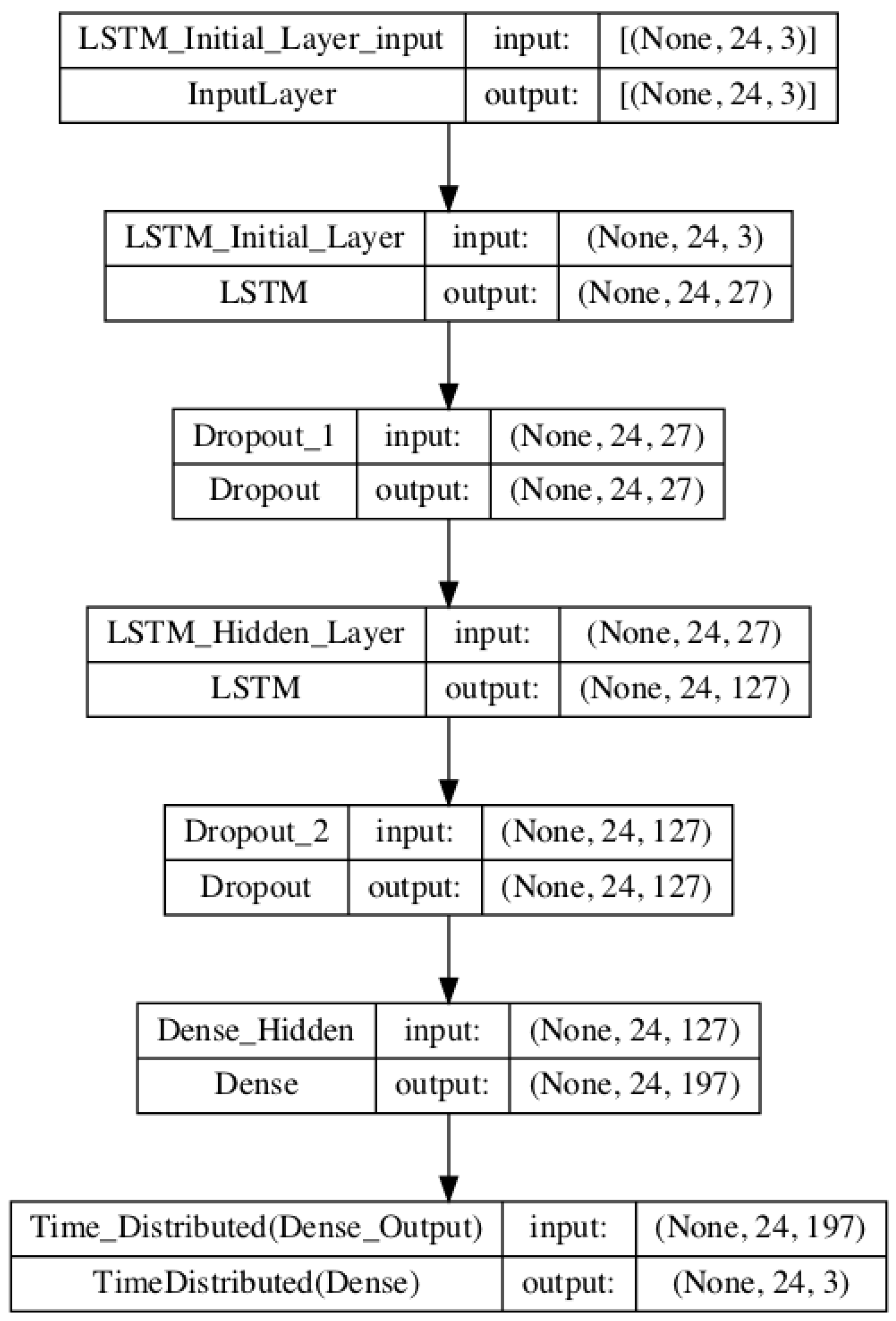
| LSTM Units Layer 1 | 27 |
| LSTM Units Layer 2 | 127 |
| Dense Units | 197 |
| Batch Size | 110 |
| Epochs | 71 |
| Learning Rate | 0.000251355666177083 |
| Dropout Rate | 0.2529847965068651 |
| L2 Regularisation | 0.000022464551680532603 |
Disclaimer/Publisher’s Note: The statements, opinions and data contained in all publications are solely those of the individual author(s) and contributor(s) and not of MDPI and/or the editor(s). MDPI and/or the editor(s) disclaim responsibility for any injury to people or property resulting from any ideas, methods, instructions or products referred to in the content. |
© 2024 by the authors. Licensee MDPI, Basel, Switzerland. This article is an open access article distributed under the terms and conditions of the Creative Commons Attribution (CC BY) license (https://creativecommons.org/licenses/by/4.0/).
Share and Cite
O’Brien, A.; Zhang, H.; Allwood, D.M.; Rawsthorne, A. From Data to Draught: Modelling and Predicting Mixed-Culture Beer Fermentation Dynamics Using Autoregressive Recurrent Neural Networks. Modelling 2024, 5, 201-222. https://doi.org/10.3390/modelling5010011
O’Brien A, Zhang H, Allwood DM, Rawsthorne A. From Data to Draught: Modelling and Predicting Mixed-Culture Beer Fermentation Dynamics Using Autoregressive Recurrent Neural Networks. Modelling. 2024; 5(1):201-222. https://doi.org/10.3390/modelling5010011
Chicago/Turabian StyleO’Brien, Alexander, Hongwei Zhang, Daniel M. Allwood, and Andy Rawsthorne. 2024. "From Data to Draught: Modelling and Predicting Mixed-Culture Beer Fermentation Dynamics Using Autoregressive Recurrent Neural Networks" Modelling 5, no. 1: 201-222. https://doi.org/10.3390/modelling5010011