
Use of Decision Trees for the Development of Decision Support Systems for the Control of Grinding Circuits


1
Western Australian School of Mines: Minerals, Energy and Chemical Engineering, Curtin University, GPO Box 1987, Perth, WA 6845, Australia
2
Department of Process Engineering, Stellenbosch University, Private Bag X1, Matieland, Stellenbosch 7602, South Africa
*
Author to whom correspondence should be addressed.
Minerals 2021, 11(6), 595; https://doi.org/10.3390/min11060595
Submission received: 12 April 2021
/
Revised: 18 May 2021
/
Accepted: 28 May 2021
/
Published: 31 May 2021
(This article belongs to the Special Issue Advances in Computational Intelligence Applications in the Mining Industry)
Abstract
:Grinding circuits can exhibit strong nonlinear behaviour, which may make automatic supervisory control difficult and, as a result, operators still play an important role in the control of many of these circuits. Since the experience among operators may be highly variable, control of grinding circuits may not be optimal and could benefit from automated decision support. This could be based on heuristics from process experts, but increasingly could also be derived from plant data. In this paper, the latter approach, based on the use of decision trees to develop rule-based decision support systems, is considered. The focus is on compact, easy to understand rules that are well supported by the data. The approach is demonstrated by means of an industrial case study. In the case study, the decision trees were not only able to capture operational heuristics in a compact intelligible format, but were also able to identify the most influential variables as reliably as more sophisticated models, such as random forests.
1. Introduction
Grinding circuits are well-known for their inefficiency and disproportionate contributions to the energy expenditure of mineral processing plants [1]. Studies have estimated that comminution circuits account for between 2–3% of global energy consumption [1,2], and up to 50% of the energy consumption on mineral processing plants [3], with the cost rising exponentially, the finer the grind. Moreover, the pronounced effect of grinding on downstream separation processes has long been a driving force for more efficient operation of these circuits through process control. However, advanced control is often hindered by the complexity of grinding operations, characterised by strongly nonlinear relationships between coupled circuit variables and long time delays. In addition, frequent changes in feed ore characteristics and other disturbances affect the operational state of the circuit, requiring frequent adjustment of set points.
This is partly the reason why in the mineral processing industry, the majority of regulatory grinding circuit control systems is realised through PID control loops [4,5]. In contrast, supervisory control functions designed to maintain set points for regulatory control and adherence to process constraints are entrusted to either process operators or advanced process control (APC) systems. The latter includes expert control systems (ECS) [6,7], fuzzy controllers [8,9], and model predictive control systems [10,11].
Despite the advantages of APC, a recent survey [12] has indicated that it is still not well-established on most mineral processing plants. As a consequence, grinding circuit performance is still largely dependent on operator decision-making processes.
Through trial and error, operators accumulate experience and heuristic knowledge to perform these supervisory functions. However, application of this knowledge is dependent on a subjective assessment of the state of the circuit and appropriate corrective action. Naturally, this can lead to inconsistent operator decision-making during similar operational states, as well as inconsistent operation between different individuals.
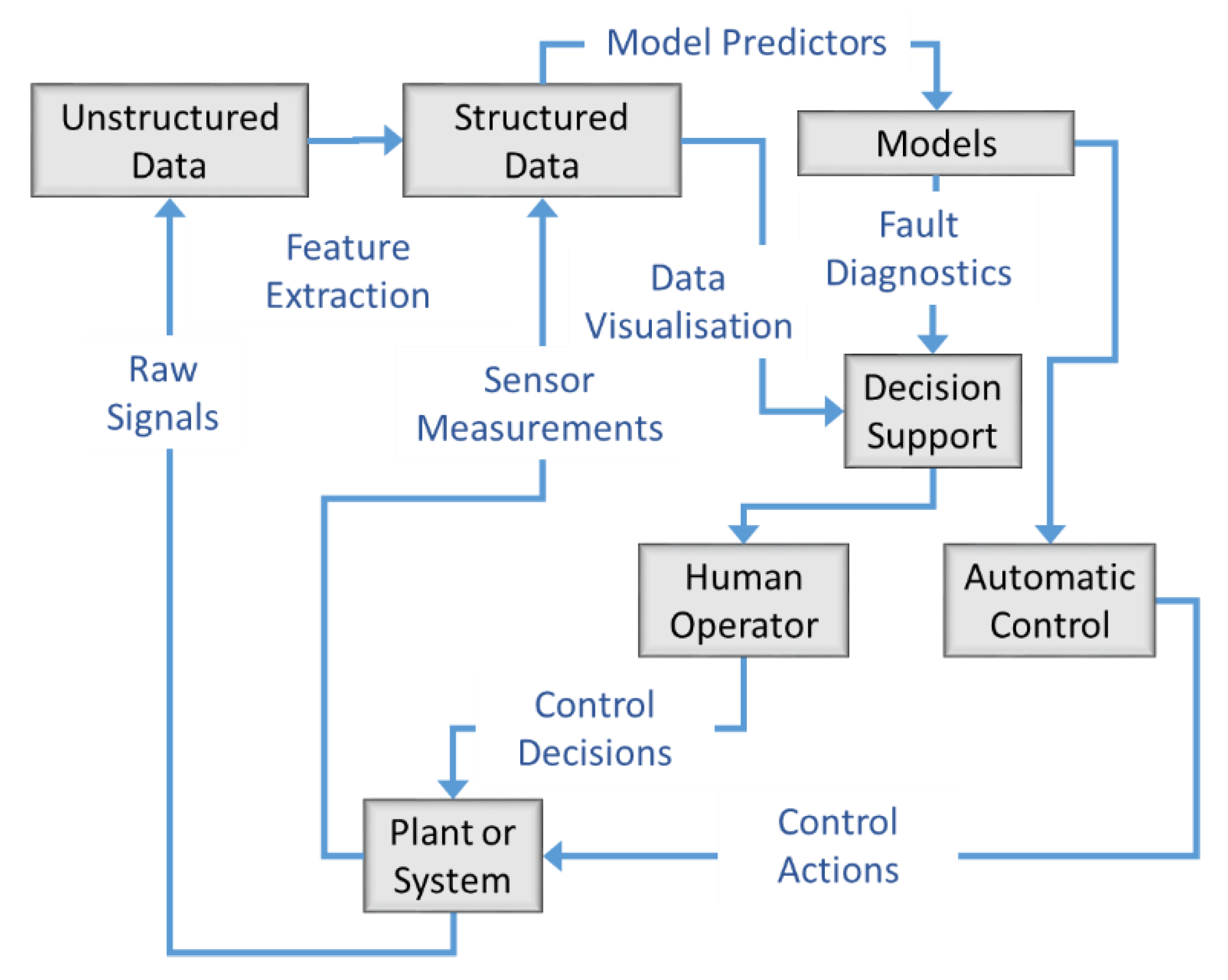
This work explores a methodology to support operator decision-making for the control of grinding circuits by extracting knowledge from plant data. Generally speaking, this may require feature extraction from raw process signals to be interpretable, which could be visualised as sets of univariate time series signals or structured data by the operator, or via more sophisticated infographic plots or displays, as indicated in Figure 1. This information may also captured by diagnostic process models designed for anomaly or change point detection or fault diagnosis, as well as models that could be used in automatic control systems, as indicated in Figure 1.
It may also be possible to build diagnostic models that could include if–then rules that could be used for higher level interpretation of the data, and it is this aspect that is considered in this paper.
More specifically, operator behaviour embedded in process data are extracted using decision trees to provide explicit and actionable rules, such as those found in ECS, presented in an if–then format. These rules are used to analyse current operator behaviour and guide future operator decisions. Application of the methodology is demonstrated in a case study using data from an industrial grinding circuit.
Section 2 provides a brief overview of knowledge discovery from data relating to grinding circuits, while Section 3 describes the specific methodology followed in the investigation, based on the use of decision trees. Section 4 demonstrates the methodology on an industrial grinding circuit, with a discussion of the results and general conclusions presented in Section 5.
2. Knowledge Discovery for Grinding Circuit Control
Control of grinding circuits requires knowledge of the fundamental principles governing circuit operation. This knowledge allows the transformation of observed data and information into sets of instructions [13]. The knowledge acquisition process is often referred to as knowledge discovery, or knowledge engineering in ECS literature [14,15].
During traditional knowledge engineering, such as used during the crafting of ECS, rules are extracted directly from the heuristic knowledge of operators or circuit experts. This is generally facilitated through interviews, questionnaires, or observation of circuit operation by the knowledge engineer [15,16]. However, situations often arise where human experts have difficulties articulating their own decision-making rationale, or the human expert knowledge is inadequate for a comprehensive knowledge-base. Alternatively, data mining tools can be applied to extract knowledge from process data through inductive learning.
Data mining usually involves fitting models to or extracting patterns from systems by learning from examples. To facilitate decision support, the specific representation of knowledge in these models are of great importance. For knowledge discovery purposes, data mining models can be categorised according to the manner in which this knowledge is represented, being either implicit or explicit [17]. Implicit representations lack the formal mathematical notations of explicit representations, thus requiring experience to understand and possibly enabling subjective interpretations.
Black box models with implicit knowledge representations have been applied successfully for grinding circuit control using neural networks [18,19,20], support vector machines [21,22], reinforcement learning [23,24], or hybrid model systems [25], among others. However, the difficulty associated with interpreting and transferring such implicit knowledge make these models undesirable for operator decision support.
In contrast, rule-based classifiers are more suitable for the development of decision support systems, as they generate explicit if–then rules that can in principle be interpreted easily by human operators. In mineral processing, rule-based classifiers include evolutionary algorithms, such as genetic algorithms [26], genetic programming [27,28], rough sets [29], as well as decision trees [30]. In addition to this, some efforts have also been made to extract rules indirectly from the data, via from black box models, such as neural networks [31,32,33,34].
Of these methods, decision trees are by far the most popular, as the rules generated by these models are easily interpretable by operators and can provide actionable steps to move from one operational state to another. These rules consist of a sequence of conditional statements combined by logical operators; an example is given below.
While this method for rule induction has been applied to numerous problems, it has found sparse application in the chemical and mineral processing industries. Saraiva and Stephanopoulos [35] demonstrated the use of decision rules extracted from decision trees to developing operating strategies for process improvement in case studies from the chemical processing industry. Leech [36] developed a knowledge base from rules induced from decision trees to predict pellet quality of uranium oxide powders for nuclear fuels. Reuter et al. [37] generated a rule base to predict the manganese grade in an alloy from slag characteristics in a ferromanganese submerged-arc furnace.
The applications of rule-based classifiers mentioned above mostly focus on the generation of rule sets for automatic control systems. Accordingly, these systems are often not suitable for interpretation by humans. In this study, the use of decision trees to extract rules from grinding circuit data that can be used to support control operators is considered. Decision trees have received some focus in the development of decision support systems, but applications to the processing industries were rarely encountered [38,39]
3. Methodology
3.1. Classification and Regression Trees
Decision trees are a class of machine learning algorithms that split the data space into hyper-rectangular subspaces. Each subspace is associated with a single class label, for categorical data, or numerical value for continuous data. These subspaces are identified by recursively searching for partitions based on a single input variable that cause the largest reduction in impurity of the output variable in the associated hyperrectangle.
Tree induction algorithms, such as CART (Breiman, et al., 1984) and C4.5 (Quinlan, 1993), utilise different concepts for this notion of impurity. Different impurity measures are also used depending on whether the tree is used for classification or regression. For classification purposes, CART, the algorithm used during this investigation, calculates the Gini Index at each split point. Consider a classification task where the proportion of class , at node , is given by . The Gini Index, , at node is given by:
The Gini Index increases as the impurity or mixture of classes increases at the node. For example, in a binary classification problem the Gini Index reaches a maximum value of 0.5 when both classes are of equal proportion in the node. A node containing examples from a single class will have a Gini Index of 0. The reduction in impurity for a proposed split position, , depends on the impurity of the current node, the impurity of proposed left and right child nodes ( and ), as well as the proportion of samples reporting to each child node ( and :
The split position resulting in the largest decrease in impurity is selected. In regression trees, splits are selected to minimise the mean squared error from predictions of the child nodes.
Without a stopping criterion specified, this procedure is repeated until all examples in a node belong to the same class, have the same response value or the node contains only a single training example. In classification models, these terminal (leaf) nodes will predict the label of the class present in the largest proportion. For regression models, leaf nodes predict the average value of all samples belonging to the node.
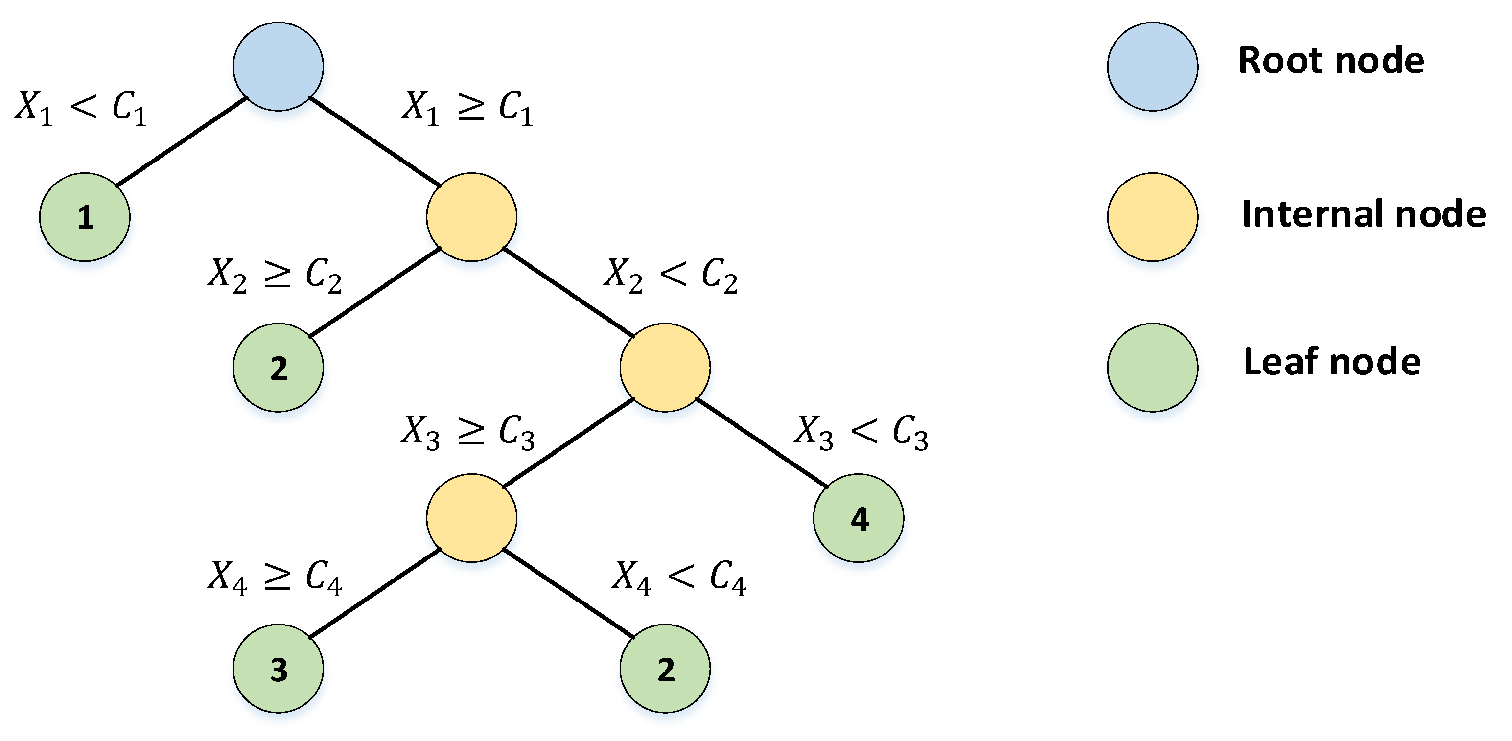
The recursive nature of tree induction algorithms allow the decision trees to be represented as tree diagrams, as shown for the classification tree in Figure 2.
The trees are readily converted to discrete normal form (DNF) [40] as sets of “if–then” decision rules by following the decision paths from the root node to each leaf node. Table 1 presents the results of this procedure illustrated for the tree in Figure 2.
Without any restrictions, decision tree models can grow to fit almost any data distribution. However, this generally results in the tree overfitting training data with reduced generalization performance. Stoppage criterions can be imposed to reduce the complexity of the tree and reduce this probability of overfitting the dataset.
These are enforced by requiring a minimum amount of samples belonging to a proposed node for the node to be formed, or placing a hard limit on the amount of allowable splits or overall tree depth.
3.2. Evaluating the Utility of Decision Rules
In this investigation, the focus was on using decision tree algorithms to extract decision rules which have significant support in the dataset and are sufficiently accurate, while remaining compact and interpretable for decision support. The utility of a rule could be considered a function of these factors, as indicated in Equation (4) below.
Conceptually, there should exist some optimal configuration of the parameters wherein the utility of a rule is maximised. This concept is explored qualitatively in the case study. Each of the three requirements are briefly discussed below.
3.2.1. Supporting Samples in the Dataset
For a rule to be of any utility, it needs to be applicable in the modelled system for significant periods of time. The higher the number of samples in the dataset belonging to a specific rule, the higher the support is for the rule, and the larger the fraction of time for which the rule is valid for decision support. This metric is analogous to the support metric used to quantify the strength of association rules [41]. An acceptable level of support for a rule is dependent on the modelling problem. When modelling common operational practices, a high number of supporting samples would be required. However, if fault or rare events are investigated, the level of support could be considerably less.
3.2.2. Rule Accuracy
The accuracy of the rule refers to the dispersion of target values of the data samples belonging to the rule. For classification trees, the accuracy of a rule is represented by the proportion of training samples belonging to the class predicted by the node. For regression trees, the accuracy is well represented by the standard deviation of the target values of samples belonging to the rule. Low standard deviation of the target values of samples indicates a relatively accurate prediction by the regression tree, with sample target values close to the predicted mean.
Both accuracy measures are closely related to the impurity measures used during construction of the trees. Ideally, emphasis is placed upon rules with high accuracy.
3.2.3. Complexity and Rule Interpretability
For a rule to be of utility for decision support, the rule must remain interpretable by humans. While this notion of interpretability is naturally subjective, longer rules with a large amount of splits are difficult to interpret and tie to physical phenomena. The shorter the rule, the easier it is to interpret and possibly act upon.
Here, the decision tree algorithm is forced to generate shorter rules, and a fewer number of rules, by specifying the maximum amount of splits allowed in the tree. However, these restrictions will come at a cost, possibly decreasing the accuracy of the rules, since the capacity of the model has been decreased. However, as will be shown, restricting the number of splits does always not have a significant effect on the model generalisation ability, while it significantly increases the interpretability of the rules.
3.3. Decision Rule Extraction Procedure
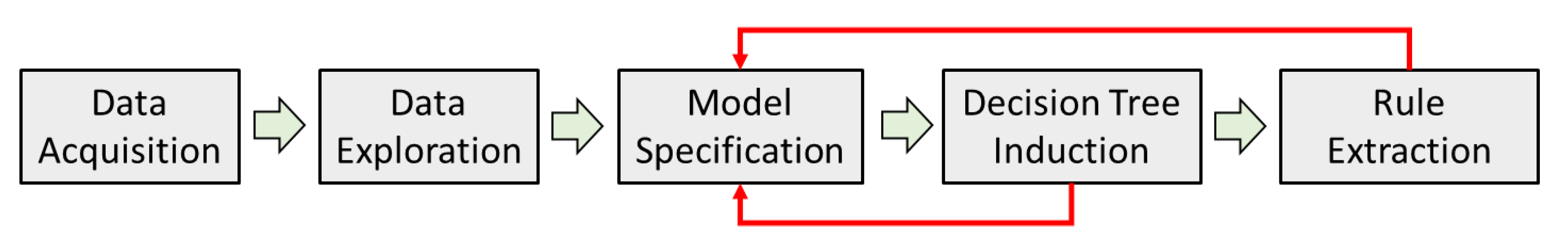
This section describes the methodology used to extract useful rules from decision trees to support operator decision-making. The overall procedure is displayed in Figure 3. The process is naturally iterative, and in practice, a practitioner would repeat the process until a rule set of sufficient utility is discovered. A short discussion of each step is presented below.
3.3.1. Data Acquisition and Exploration
Operational data is collected from a mineral processing plant. Ideally, this dataset would span a period of operation capturing some variation or drift in the process. To successfully evaluate the utility of identified rules, the practitioner has to be very familiar with the intricacies of the operation, or a circuit expert needs to be consulted. Next, an exploratory analysis of the collected data can be conducted. The presence of frequently recurring operating states are identified and the conditions around these states inspected. Tying decision rules to specific operational states could provide guidance to move from less, to more favourable states.
3.3.2. Model Specification and Tree Induction
The modelling problem needs to be carefully formulated to ensure rules are extracted to address a specific variable that can solve an existing problem, or address specific operational patterns. This leads to the identification of candidate input, , and target variables, , for the decision tree algorithm.
Both controlled and manipulated variables are suitable targets for knowledge discovery. Decision tree models constructed with manipulated variables as the target leads to rules with a direct control action as its prediction. Modelling a controlled variable does not have this feature, but serves to discover common operational patterns leading to different operational states.
In addition to traditional operational variables, the role of the operator is embedded as a latent variable into the dataset. The operator’s contribution will usually be revealed as a set point change in the manipulated variables. Thus, in many situations rules are actually describing common decision-making patterns by operators.
Once the input and output variables are designated, decision trees are induced on a training partition of the data, and a test set is used to measure the generalisation ability of the tree. If the accuracy of the tree proved to be too low, previous steps were repeated. Variable importance measures were used to quantify the relative contributions of different variables to the model. The results should be evaluated for consistency with heuristic circuit knowledge.
3.3.3. Rule Extraction and Evaluation
Decision trees are readily converted into a DNF rule set. In a decision tree, each path from the root node to a terminal node can be represented as a rule consisting of the conjunction of tests on the internal nodes on the path. The outcome of the rule is the class label or numerical value in the leaf node. Such a rule is extracted for each terminal node in the decision tree.
The utility of each rule was evaluated using the measures proposed above. Rules with high utility are considered valuable for operator decision support and were further analysed for the knowledge the rule contains and its practical usage.
4. Case Study
In this section, the methodology is applied to a dataset from an industrial semi-autogenous grinding (SAG) circuit. The circuit is operated under human-supervisory control, with set points primarily determined by process operators based on production targets from management. Classification trees were used to analyse the operational patterns surrounding periods wherein the mill overloaded, requiring drastic action from process operators. Identifying and addressing the circuit operating patterns during such events could reduce the frequency of similar events in future operation.
4.1. SAG Circuit Description
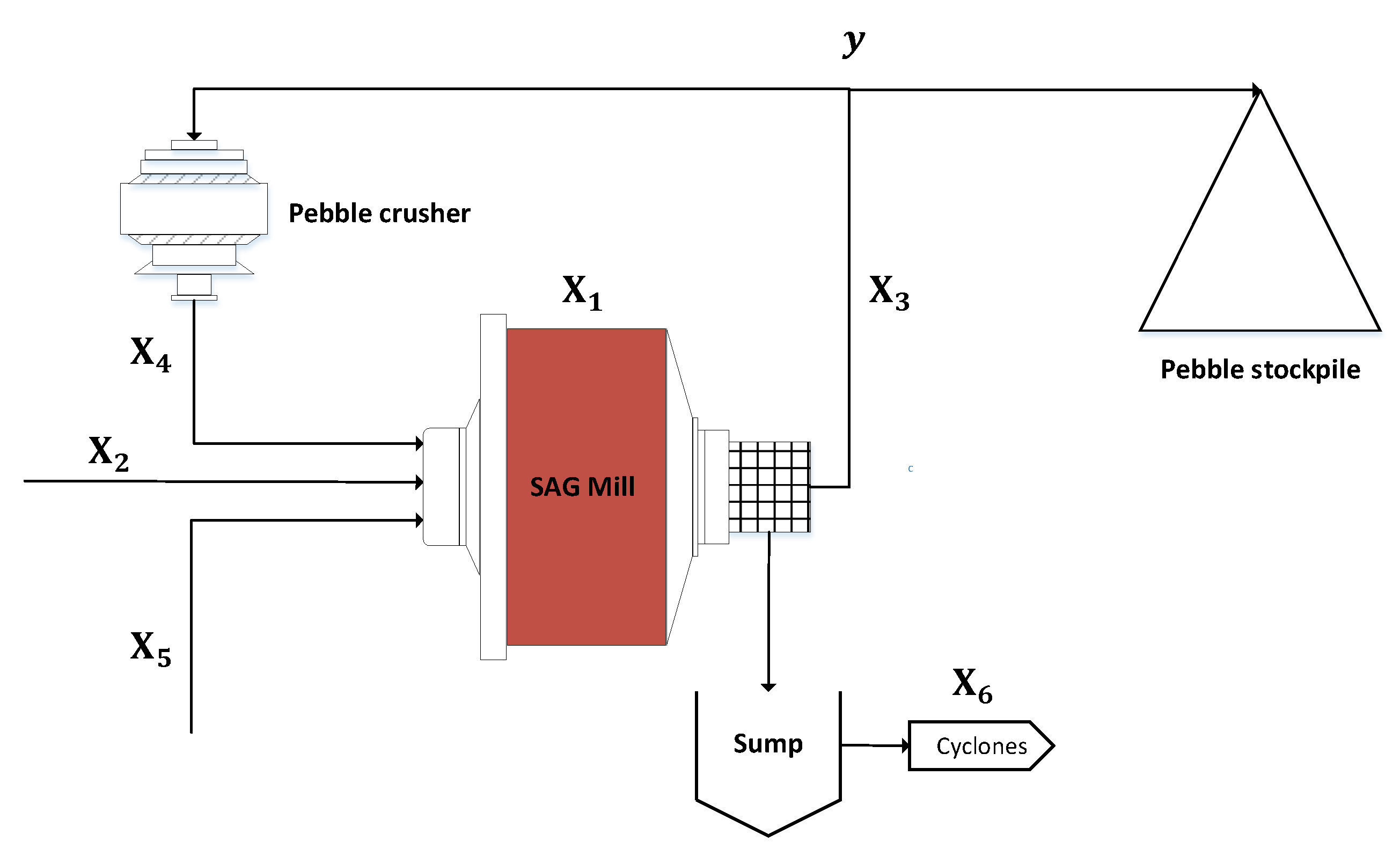
A schematic of the SAG circuit is shown in Figure 4. Crushed ore and water are fed to the SAG mill. Fine SAG mill product leaves the mill through a trommel screen and enters a sump before being pumped to a reverse configuration ball milling circuit. Pebbles, consisting of the mid-size fraction material building up, exit the mill through pebble ports and crushed in a cone crusher before being fed back to the mill.
The SAG circuit is operated to achieve maximum throughput, by maximising dry feed rate, while operating within the power draw limits imposed by the SAG mill drive system. Operators continuously monitor the mill power draw and respond by changing the feed rate accordingly. Distinction is made between the pebble discharge, , and pebble returns rate, , since operators have the option to drop the whole pebble stream to a stockpile, allowing near instantaneous mill load control.
4.2. Modelling Problem Description
In this case study, the focus was on gaining an understanding of the sequence of events leading to operators deciding to bypass the pebble circuit. It was generally understood that these events occurred in reaction to impending mill overloads, by removing the mid-size fraction from the mill charge. However, metallurgists wanted to discover common operating patterns leading to these overload and subsequent pebble circuit bypass events.
While dropping the pebbles to a stockpile can dramatically reduce the mill load, and subsequently power draw, this action essentially just postpones the problem. Generation of the pebble material has consumed significant amounts of energy, without resulting in product sent for downstream concentration. The pebbles contain a significant amount of valuable material that will require regrinding in the future. Additionally, the drastic change in mill load results in a coarser overall grind and forces the mill into subsequent cycles of instability.
Accordingly, the modelling problem was formulated to predict the status of the pebble circuit as a function of the remaining operational variables. The model specification is summarised in Table 3.
Since the status of the pebble circuit can be represented as a binary “on/off” variable, the problem was suitable for a classification model. Alternatively, modelling the variable as a regression target should lead to similar results.
Notably missing from the inputs in Table 3 is , the pebble returns rate. Pebble circuit bypass events correspond to normal tonnages on , but no pebble returns to the feed conveyor (zero on ). Thus, the status of the pebble circuit can be perfectly predicted from knowledge of and alone. Combining these two variables in a model will result in perfect predictions, but no meaningful insights will be obtained from decision rules.
Since it is a manually triggered event, modelling the status of the pebble circuit essentially attempts to model the operators’ decision-making processes. Decision rules induced during the analysis should identify the most common operational patterns leading to bypass events. Once these patterns are identified, the behaviours can be addressed in an attempt to decrease the frequency of these occurrences.
4.3. Raw SAG Circuit Data Exploration
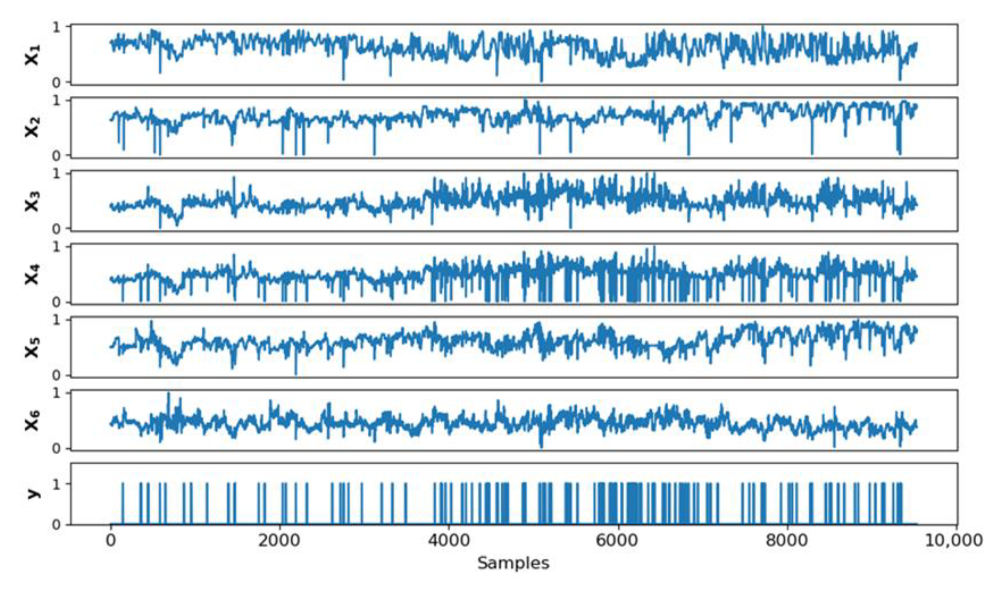
Data samples were collected at a frequency of 5 min from the plant spanning a period of approximately six weeks of operation. The normalised data samples are shown in Figure 5. Regarding the binary variable , a bypass of the pebble circuit is designated with the value 1, while normal operation of the circuit is denoted with the value 0. From the 9500 samples present in the dataset, 435 samples corresponded to periods of bypassing the pebble circuit, from 141 unique bypass events. The data were cleaned to remove downtime and any equipment maintenance periods.
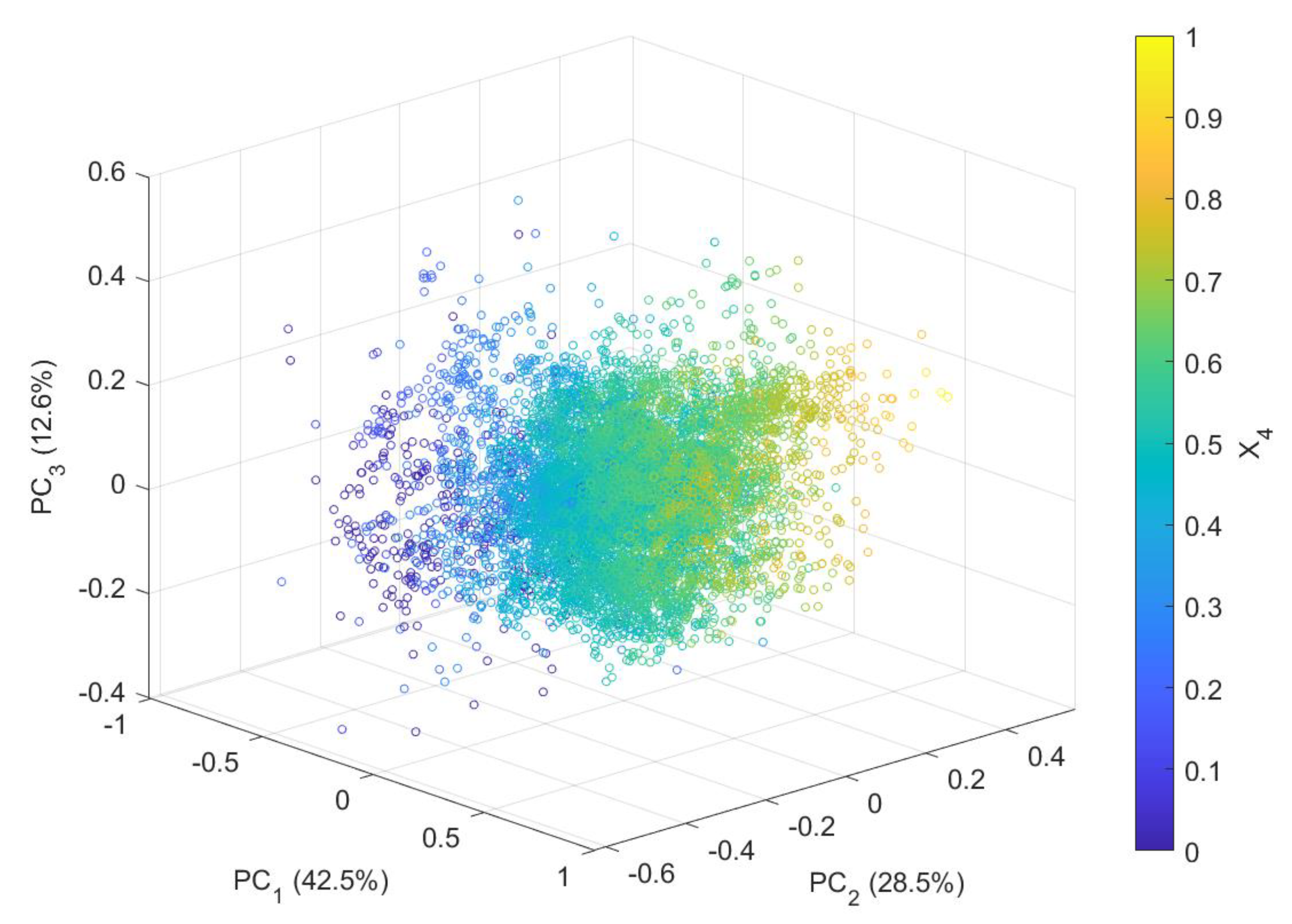
Figure 6 shows the effect of the pebble circuit bypass on the overall variability in the circuit. The figure shows the principal component scores of the dataset on the first three principal axes, with the pebble returns superimposed as a colour map. Bypassing the pebble circuit corresponds to no pebbles returned to the mill. From the figure, it can be seen that periods of bypass lie outside the edges of the central cluster of normal operation. This suggests that reducing the frequency of these events would decrease the overall variability in the SAG circuit.
4.4. Random Forest Classification Model
To gain a baseline indication of the predictability of the power draw from other circuit variables, a random forest model [42] was trained for the classification task. The random forest model, consisting of the bagged ensemble of trees and bootstrap samples used to train each tree in the forest, provides an upper limit for comparison to the predictive performance of individual tree models. Variable importance estimates from random forest models are also generally more reliable than decision trees because of the bootstrap aggregating procedure.
A random forest model was trained for the classification task specified in Table 3, using the parameters summarised in Table 4. The number of trees in the forest was selected to be large enough such that a further increase in the number of trees does not increase the model generalization. The number of predictors to sample at each split in the tree, from the total number of variables , was maintained at the default value as suggested by Liaw and Weiner [43].
The dataset was split into a training and test dataset in an 80/20 ratio. Since the number of bypass events are highly outnumbered by normal operation, the target dataset was highly imbalanced. The imbalance was negated by imposing a higher misclassification cost on bypass samples misclassified as normal pebble circuit operation. The higher misclassification cost was set equal to the proportion of normal samples to pebble circuit bypass samples, to reduce the amount of predictions resulting in false negatives. The custom cost matrix is shown in Table 5.
To quantify the model accuracy on the imbalanced dataset, the F1-score was used, as defined below:
In this context, the precision designates the fraction of samples correctly classified as bypass events (true positives) against the total number of samples classified as bypass events (true positives and false positives). The recall designates the fraction of samples correctly classified as bypass events (true positives) against the actual number of bypass event samples (true positives and false negatives). Ideally, a model should obtain high precision and recall. Since the F1-score is simply the harmonic mean of these two measures, a high F1 score is also desired.
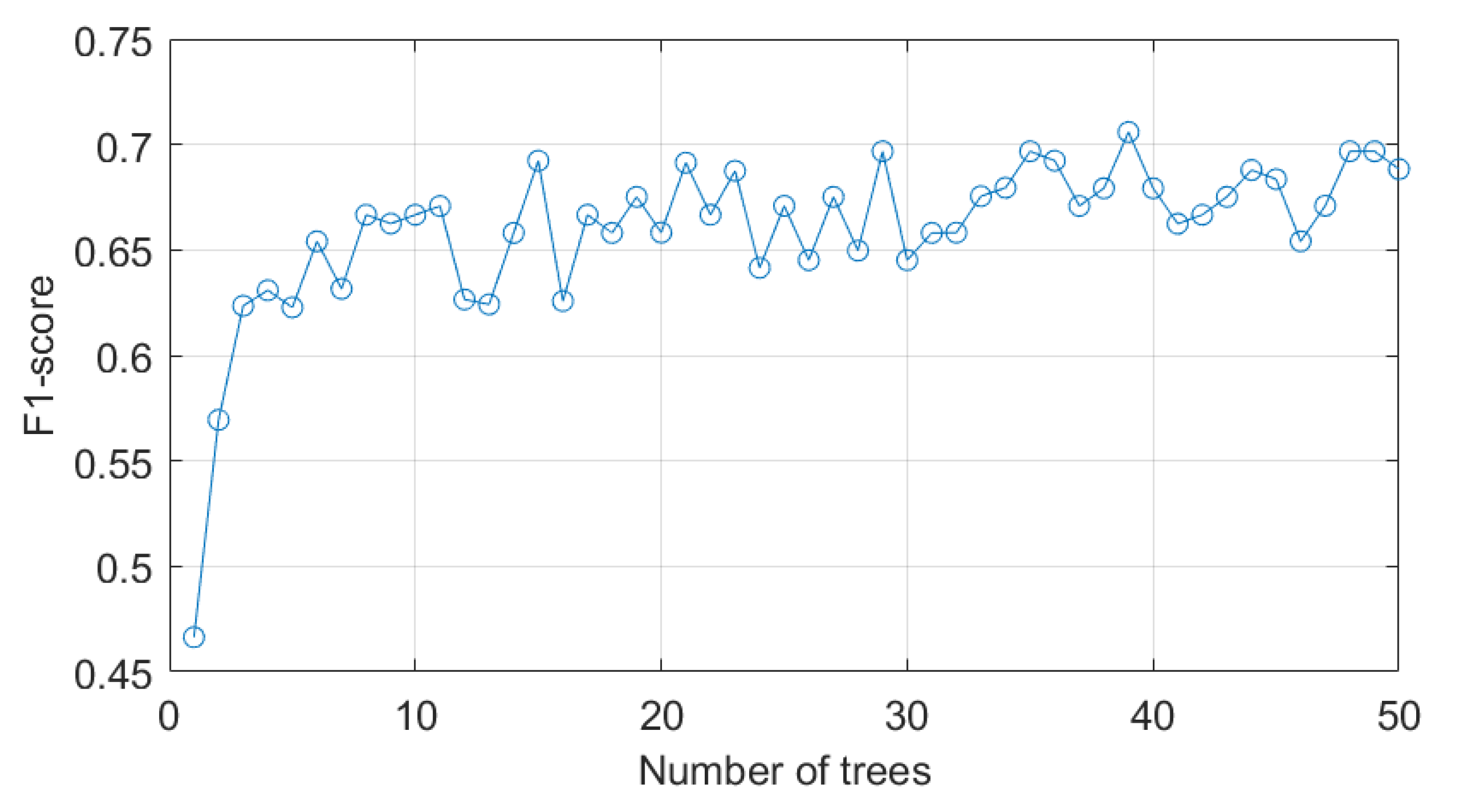
The F1 score as a function of the number of trees in the random forest model, as calculated on the held-out test set, is shown in Figure 7. The figure demonstrates that the F1-score improves sharply until ten trees are added to the model, after which the score plateaus around 0.7 and less significant increases to the generalization performance is observed. Notably, a single decision tree achieves a F1-score of only 0.47, indicating a significant number of misclassifications.
The misclassifications are shown in the confusion matrix in Table 6 for a random forest with 50 trees. The confusion matrix shows that the model predicts a low number of false positives, corresponding to a precision of 0.77. However, a significant number of false negatives, corresponding to a recall of 0.6, arises because of misclassification of actual bypass events.
The results demonstrate the difficulty of classifying the pebble circuit bypass events. This is likely a consequence of the fact that the model is attempting to describe operator decision-making. While it is thought that there is a general pattern leading to these events, the decisions made ultimately rely on subjective assessments of conditions and inconsistent choices between different individuals. The complexity of the modelling task is further increased by the general uncertainty present in the circuit, related to the disturbances of feed ore characteristics. However, the majority of the events are correctly classified, and the rule extraction procedure can be used to identify the most prominent behavioural patterns leading to these events.
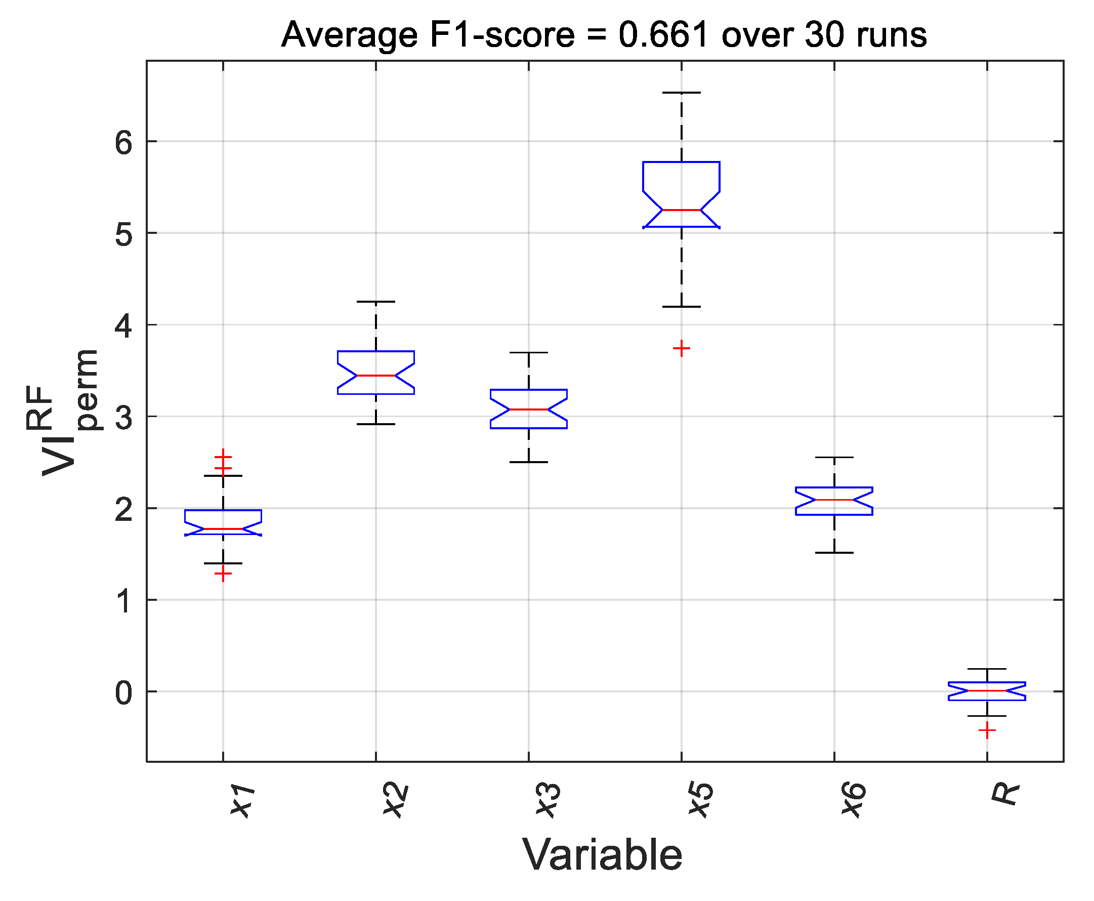
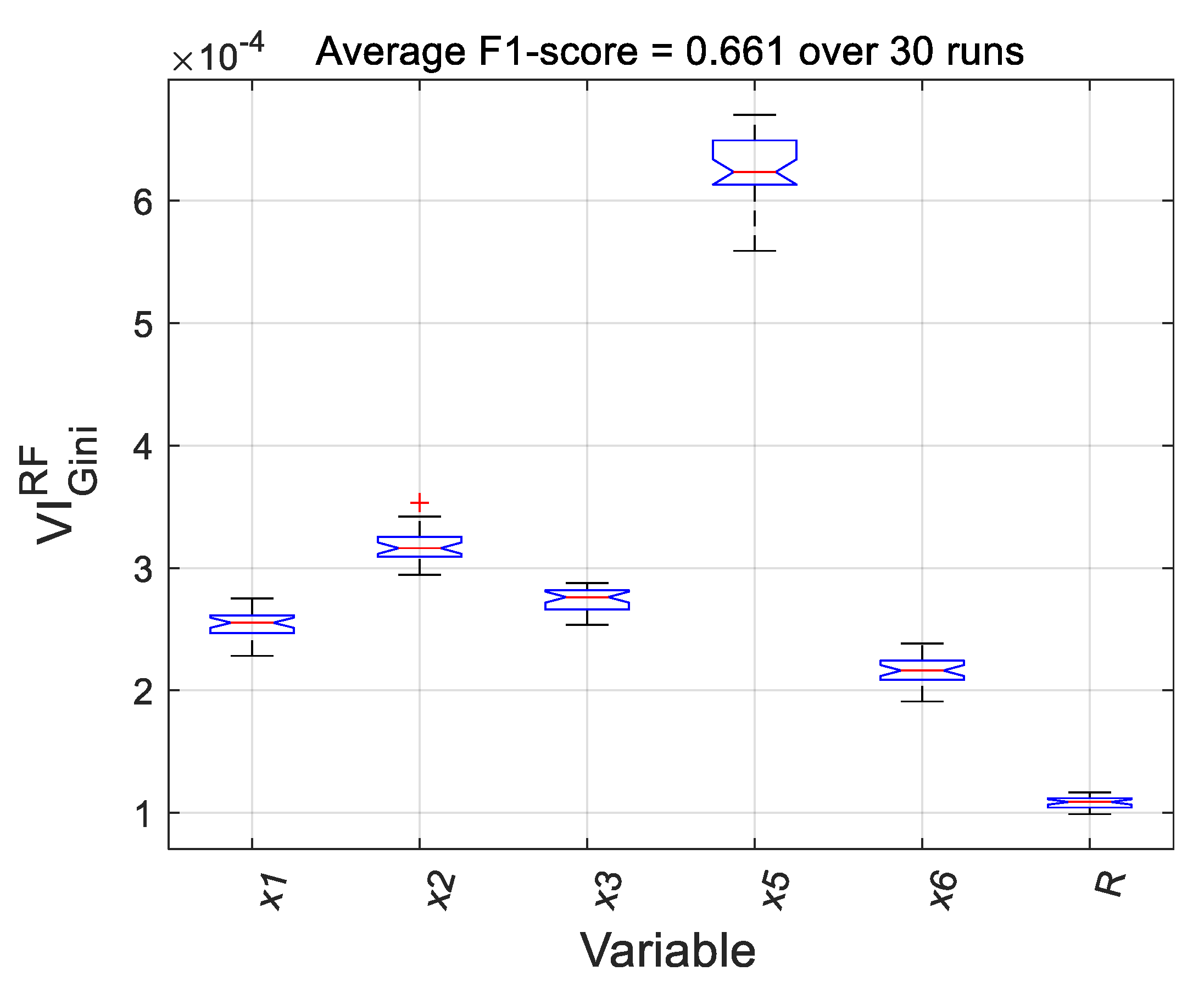
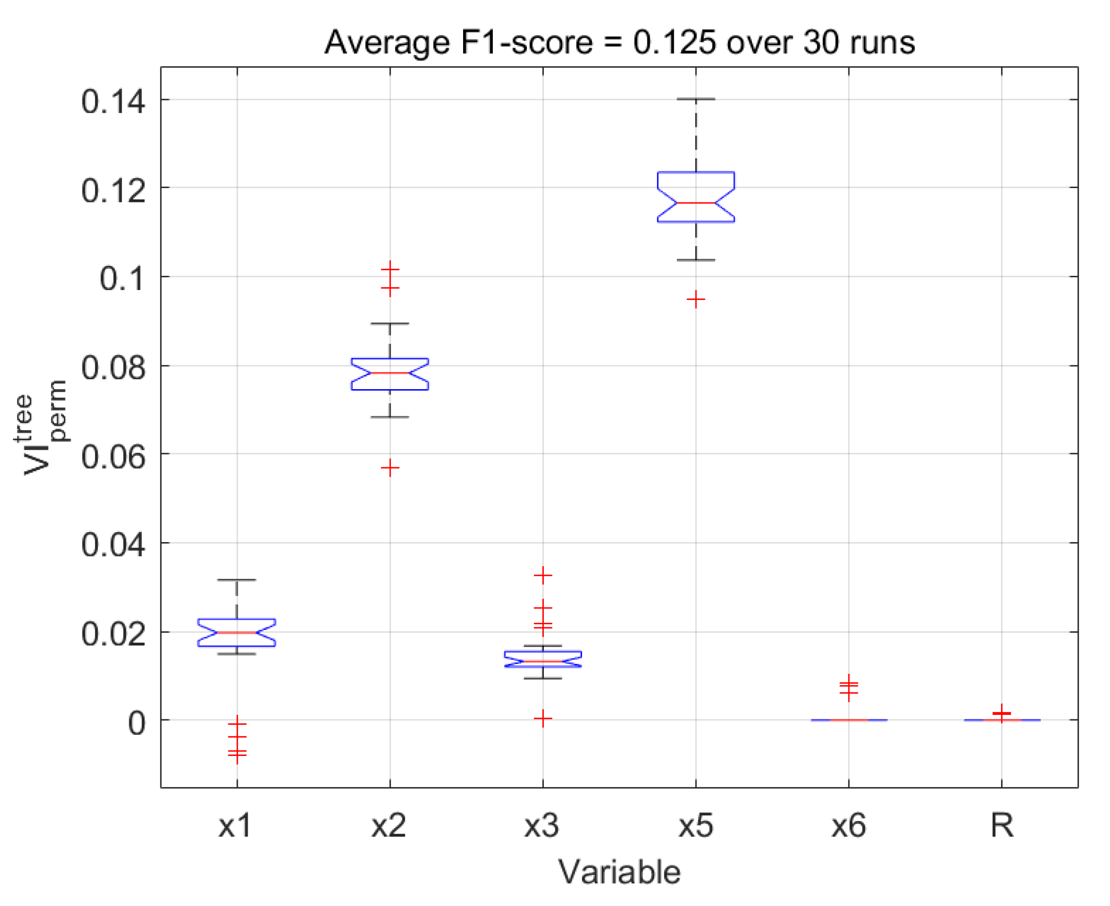
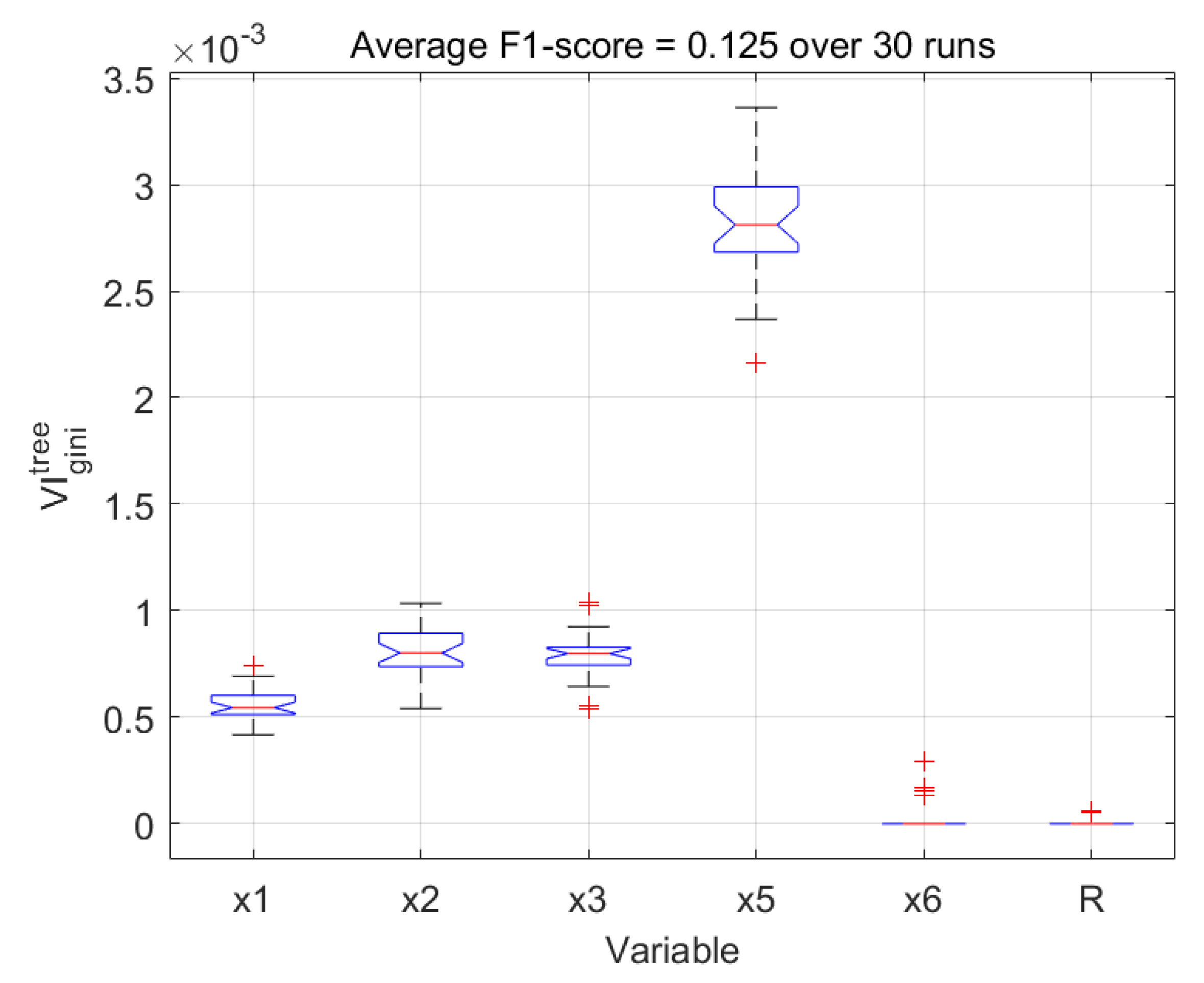
The permutation importance and Gini importance measures [42,44] were calculated to quantify the importance of each variable in the random forest model. A random or dummy variable was added to the set of predictor variables, as was proposed by [45]. This random variable had no relationship with the target variable and serves as an absolute benchmark against which to measure the contributions of the variables. Both measures were calculated for 30 instances of the model, with each instance trained on a different subset of the data. The distributions of the importance measures calculated based on the permutation importance and Gini importance criteria are shown in Figure 8 and Figure 9, respectively. In these figures, the red horizontal bars in the centres of the boxes show the median values of the importance measures, while the upper and lower edges of the boxes correspond with the 25th and 75th percentiles of the measures. The whiskers extend to the most extreme points not considered outliers, which are indicated by ‘+’ markers. The notches in the boxes can be used to compare the median values of the importance measures, i.e., non-overlapping notches indicate a difference between the median values of the importance measures with 95% certainty
In both figures, all variables contributed significantly more to the target variable than the random variable. Both measures shows markedly similar variable importance distributions. Both measures identify significant model contributions from , the water addition rate, and , the dry feed rate. A lesser contribution from , the pebble discharge rate, is noted. Although the pebble circuit bypass is generally thought to be a response to rapid increases in the power draw, this variable was deemed less significant.
Ideally, a decision tree analysed for decision support should prioritise the same variables as the random forest model. Apart from the F1-score, a similarity in the variable importance distributions serve as additional indication that the structure of a decision tree is sufficiently representative of the more accurate and robust random forest model. Accordingly, these measures were compared with the variable importance measures obtained from a single decision tree, as demonstrated in the next section.
4.5. Decision Tree Induction and Simplification
The previous section demonstrated that the status of the pebble circuit is to an extent predictable from the set of input variables. The RF model demonstrated that a F1-score of 0.47 could be obtained using a single decision tree. While this constitutes a considerable drop in accuracy from the unrestricted random forest model, simpler decision tree models should still be able to extract simple rules describing the most common patterns leading to bypass events.
The trees in the random forest model are constructed without any restrictions on tree or branch growth. This impedes the extraction of short, interpretable decision rules from the tree.
A decision tree model was trained for the classification problem using the parameters in Table 7 below. A restriction on the minimum parent (branch) node size is usually imposed as a default setting in software packages to prevent the tree from growing separate branches for each training example. However, the minimum leaf size of one member still allows the tree to overfit the training data.
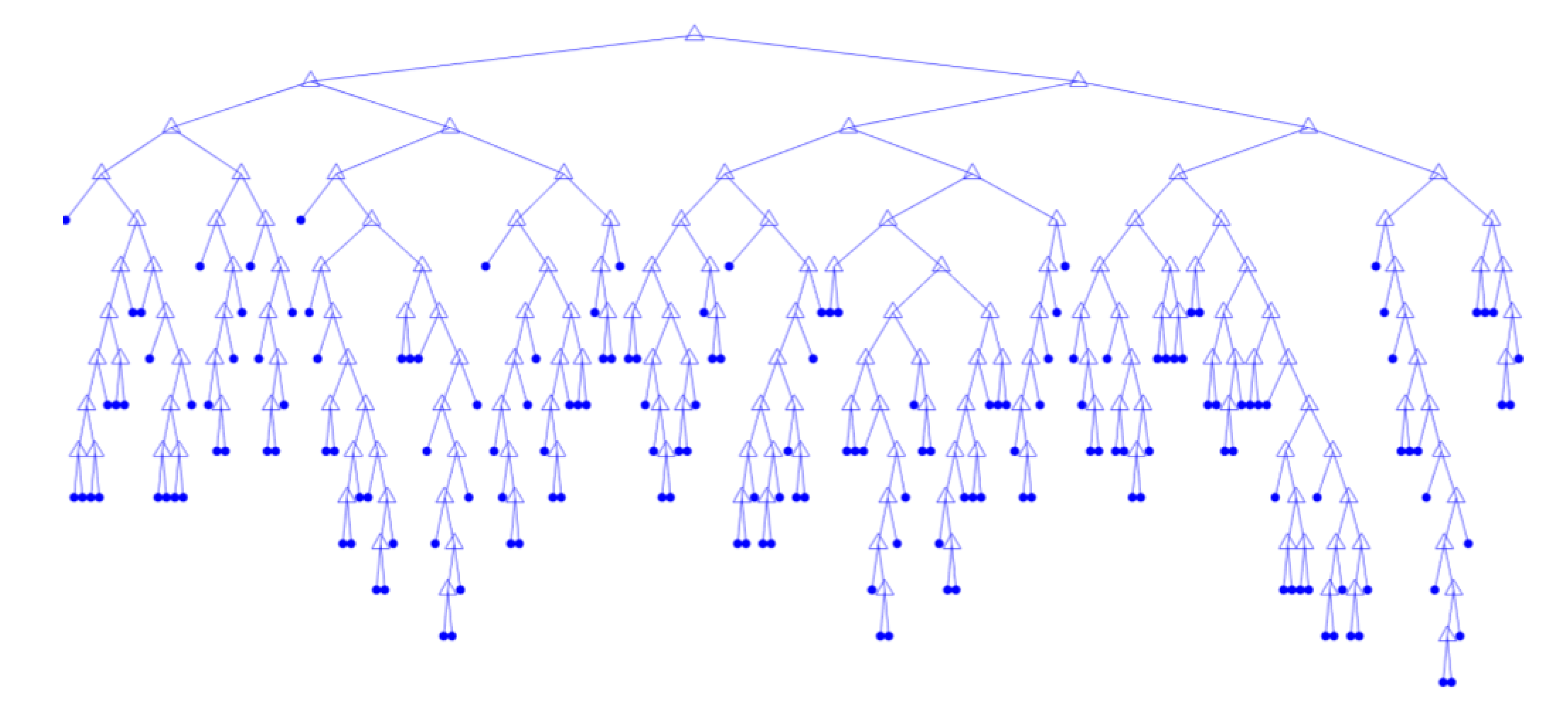
A decision tree trained using the parameters in Table 7 is shown in Figure 10. With no restrictions placed on the branch growth, the tree contains 173 branch nodes and 174 leaf nodes. The tree achieved a classification accuracy, in terms of the F1 score, of 0.422.
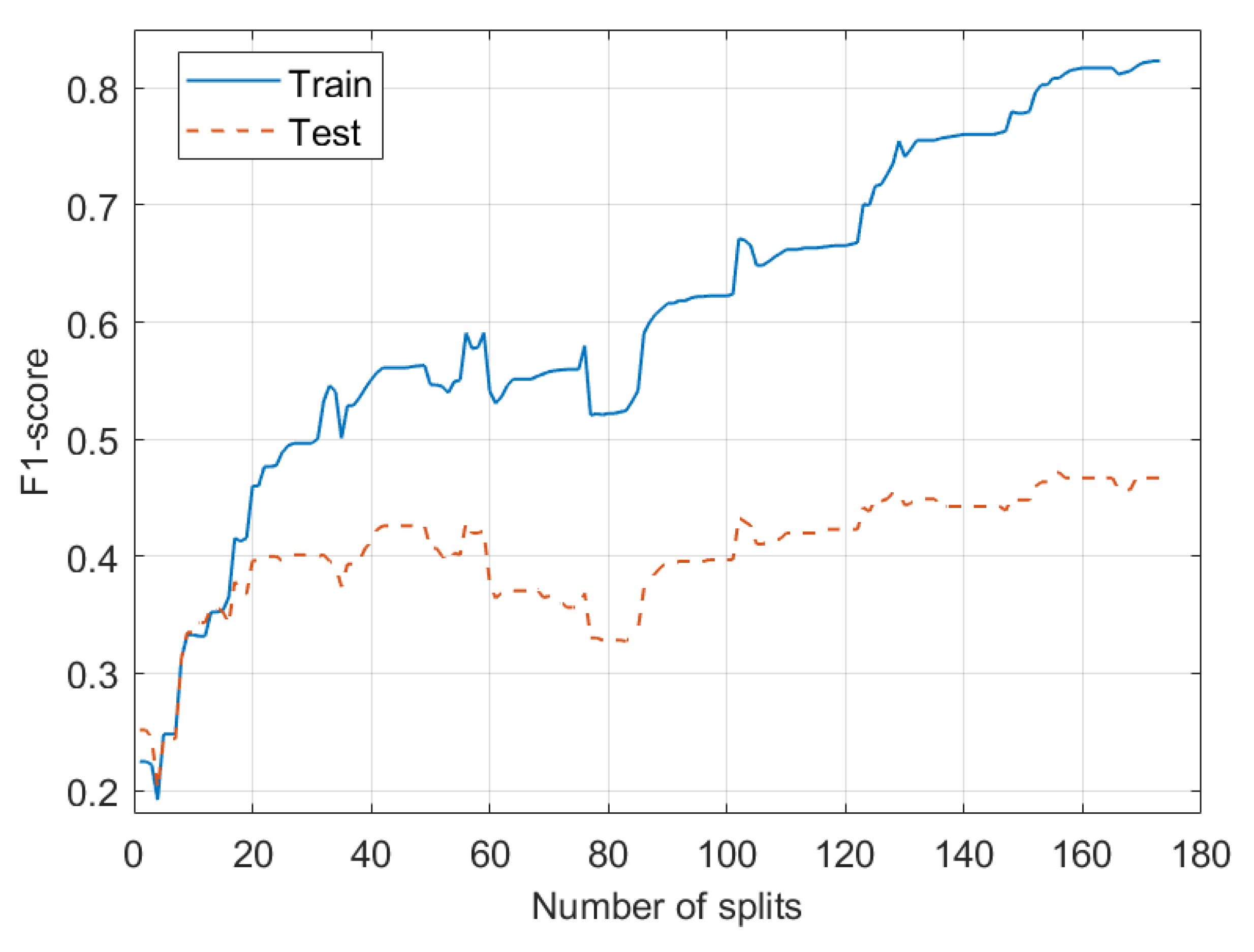
While the large number of splits and leaf nodes allow the tree to more closely fit the training data, the interpretability of the decision tree and individual tree branches is lost. The absence of restrictions on tree splitting parameters, such as the number of splits or tree depth, also reduces the generalisation ability of the tree by overfitting to the training dataset. This is demonstrated in Figure 11, where the training and test set accuracy of a decision tree is plotted as a function of the maximum number of splits allowed.
Figure 11 shows a slight increase in the F1-score on the test set with increasing number of splits. There is a sharp increase in the F1-score up until 20 splits, after which the increases become less significant. However, even at 20 splits, the F1-score is only 0.4, indicating a significant number of misclassifications. This stresses the importance of the accuracy of rules extracted from such a tree.
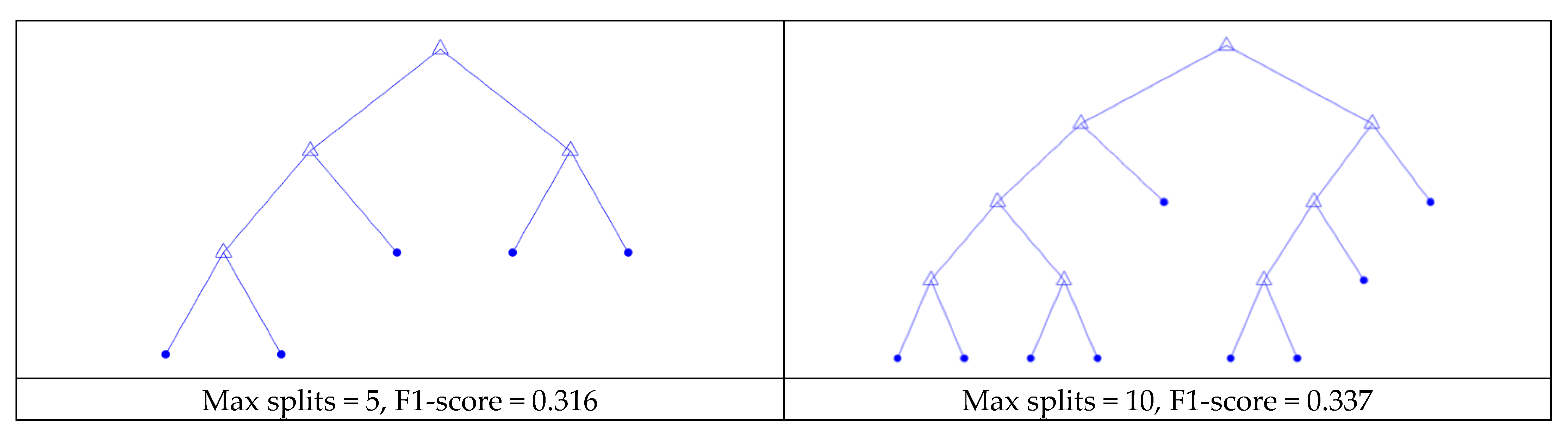
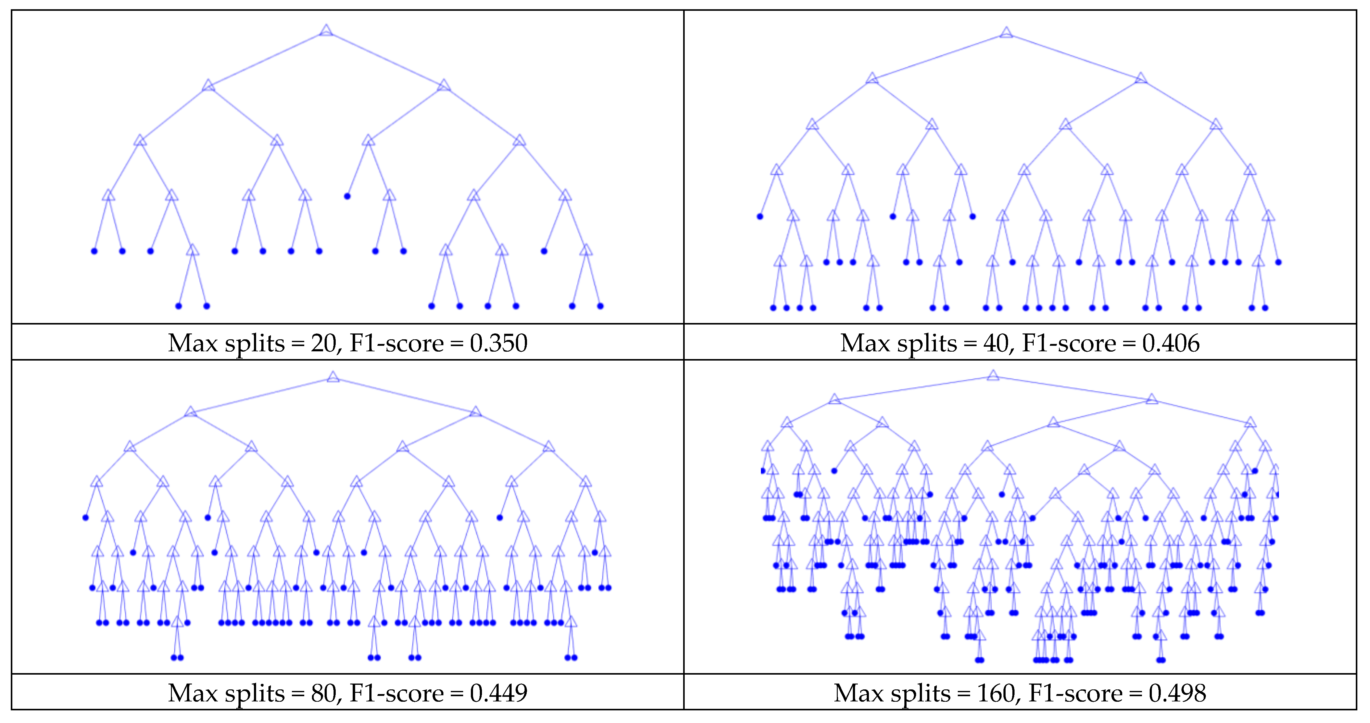
Further, Figure 11 shows that above 20 split nodes the tree is starting to overfit the training data with only marginal increases to the generalization ability. This result indicates that we can significantly reduce the number of splits for construction of the decision trees, while maintaining acceptable accuracy and generalisation ability. Restricting the number of splits and leaf nodes will somewhat decrease the reliability of the tree, but will also simplify the tree branches greatly to allow the extraction of interpretable decision rules. This simplification is demonstrated in Figure 12.
The trees in Figure 12 were constructed with the parameters indicated in Table 7, as well as an additional parameter restricting the maximum number of splits allowed in the tree. The figure demonstrates that small numbers of short, interpretable rule sets can be generated with 20 or less splits in the tree, while maintaining acceptable accuracy on the test dataset.
For illustrative purposes, the rest of the analysis considers a tree with ten split nodes. Table 8 shows the confusion matrix for such a tree, which achieved an F1-score of 0.331. Because of the increased misclassification cost, the majority of bypass events are correctly classified. However, this also leads to an increased number of false positives.
The above tree induction was simulated 30 times and the variable importance measures were calculated at each iteration. The permutation and Gini variable importance measures are shown in Figure 13 and Figure 14, respectively. Both measures rank the importance of the input variables similarly to that of the random forest model in Figure 8 and Figure 9. However, the importance of the hydrocyclone has diminished in the underfit decision trees. All inputs are again at least as important as the random variable.
The average F1-score over the 30 model instances is notably lower than the above result. This demonstrates the sensitivity of the generated models to the specific partition of data used during training.
The variable importance measures were calculated to directly compare with the results in Figure 8 and Figure 9. This analysis is required to analyse the importance of variables in a random forest, since the forest of trees obstructs simple interpretation of the model. However, a single decision tree is more interpretable, and the most significant variables should be recognisable from the top branches in the tree.
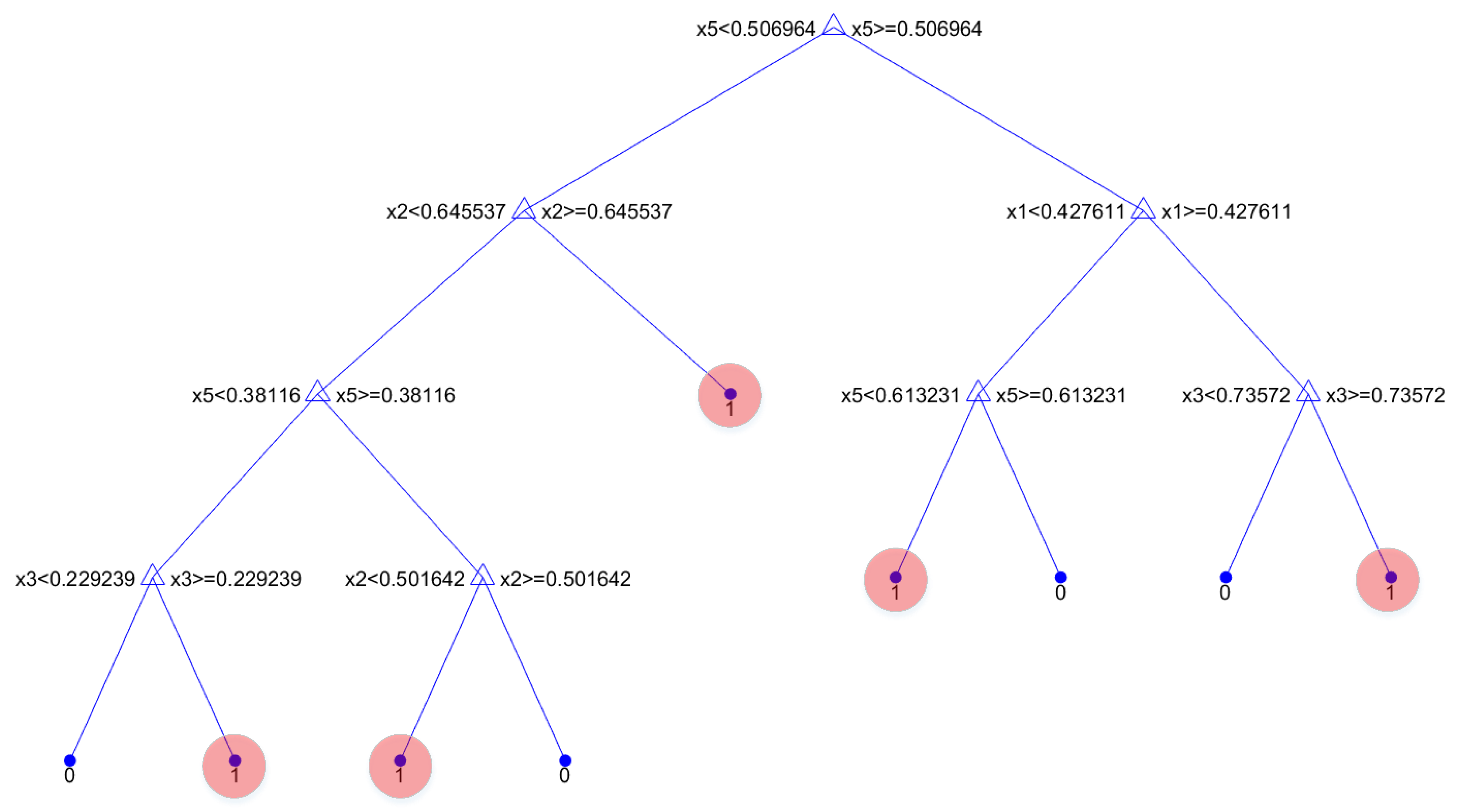
The tree corresponding to the results in Table 8 is presented in Figure 15. The variables close to the root node in the tree correspond to those identified as most significant by the variable importance measures. In the following section, decision rules are extracted from this tree and analysed for their utility in decision support.
4.6. Extracting and Evaluating Decision Rules
The pathways from the root node to leaf nodes in the tree in Figure 15 are represented as decision rules in Table 9. Where the pathway contains multiple partitions on the same variable, the rule was simplified to contain a single expression for each unique variable. The support, accuracy and number of splits for each rule is summarised in Table 10, with which the utility of each rule could be evaluated.
The rules in Table 9 leading to bypass events naturally have relatively small numbers of supporting samples because of the prevalence of these events, and this state essentially representing fault conditions. In Table 10, the rules predicting bypass events all have an accuracy below 0.5. If the prediction was a simple majority vote of all the samples belonging to the rule, the rules would naturally predict normal operation of the pebble circuit. However, the higher cost imposed on misclassifying actual bypass events outweighs the cost of misclassifying normal operation samples. Thus, the higher misclassification cost allows for the identification of the operational states wherein these bypass events are most likely to occur. Intuitively, the accuracy is thus better interpreted as an indication of the probability of a bypass event occurring in the operational state specified by the rule. The number of splits are low and interpretable because of the maximum number of splits restriction imposed on the decision tree.
Three of the rules extracted are critically analysed below. Consider a closer inspection of rule 5:
The rule states that at a higher dry feed rate coupled with a lower water addition rate, corresponding to an increased solids density in the SAG mill, there is a 36% chance the circuit would be bypassed. Depending on ore characteristics at the time, the inadequate water addition is causing the mill to retain more fines than usual, leading to an increase in the mill load and power draw. To decrease the probability of this event in the future, metallurgists could reconsider the SAG discharge density targets given to operators based on different ore sources.
Rule 9 states the following:
Rule 9 states that when the water addition rate and power draw are at medium levels or higher, while the pebble discharge rate is high, there is a 10% chance that the pebble circuit would be bypassed. This situation might arise when the mill feed suddenly changes to a more competent ore source, or a larger portion of mid-size fraction material is being fed. The mill load and power draw are not necessarily high, but the fraction of mid-size material being discharged from the mill is increasing, possibly to a level where the pebble crusher and circuit conveyors are unable to deal with the increased load. Depending on the mill fill level and the amount of power available, operators might choose to draw a higher portion of large rocks from the stockpile to attempt to break down some of the mid-size material. Alternatively, operators may choose to draw an increased fraction of finer material from the stockpile to maintain the mill throughput while not further contributing to the generation of pebbles. Metallurgists could further investigate the particle size distributions received from the preceding crusher section to deal with these occurrences.
Rule number 9 is directly contrasted by rule 8, which received the highest amount of support in the dataset:
As seen in the tree in Figure 15, rule 8 and rule 9 split the data space according to the specific value of the pebble discharge rate. In contrast to rule number 9, rule 8 predicts that at lower pebble discharge rates, the circuit was only bypassed 1.1% of the time. Thus, the combination of the two rules discover the explicit value of the pebble discharge rate, such that when this value is exceeded, the operator is ten times more likely to bypass the pebble circuit. The rule can alert an operator when approaching this specific operational state, hopefully triggering faster control action and avoiding the bypass event.
5. Discussion and Conclusions
In the case study, classification trees were used to model operator decision-making, when deciding whether to remove the critical size material from the circuit to prevent the mill from overloading. It was demonstrated how the model specification can be exploited to identify the causes of rare events. It was demonstrated that rules can be extracted to understand why and when operators were making this particular decision.
This type of knowledge can be utilised by metallurgists to aid in determining circuit operational parameters, or provided to the operator as decision support on a human-machine interface (HMI). Decision support on a HMI could nudge the more cautious operator to increase throughput, or restrain aggressive operators when their ambitions might push equipment towards its limit and require drastic action. This decision support could take the form of explicitly displaying rules extracted on a HMI, or process alarms alerting the operator when entering a state governed by a specific rule. Depending on the specific problem investigated, such decision support systems could either increase overall throughput, increase the energy efficiency of the grinding task, or reduce the wear to mill consumables and liners.
The merits of this type of rule induction is based on its simplicity. Site experts or metallurgists can identify a problem and formulate a model to answer questions regarding the problem. Rules are then easily induced using pre-packed CART implementations. There is no guarantee that the rules will contain valid or insightful knowledge, so the expert is required to critically analyse to ensure they are reasonable. The greatest inhibitor of extracting rules for successful decision support would be the unavailability of quality data sets, or a lack of site-specific knowledge to interpret and critically evaluate the patterns such rules discover. Neither of these should be of any concern to a plant metallurgist.
While it is unlikely that this induction is used for the generation of a complete ECS, it can certainly augment heuristic knowledge from experts in such systems. Experts often have difficulty explaining the procedures they follow to arrive at decisions [15]. Rule induction could aid in formalizing some of the procedures.
As noted by Li et al. [46], the integration of human operators and technology in the control room is lacking in the minerals processing industry. The successful implementation of any process control or decision support system is reliant on effective HMI visualisations, and training operators to effectively utilise such tools.
In summary, decision trees can be used as an effective approach to extract intelligible rules from data that can be used to support operators controlling grinding circuits. Three criteria are considered in the process, i.e., the accuracy of the rule, the support of the rule, and the complexity of the rule. While the case study described the application of classification trees, the methodology is easily extended to regression problems.
In addition, in some instances, as was the case in this investigation, they can be used to identify the most influential variables as reliable as more complex models, such as random forests.
Future work will focus on the industrial operationalization of the approach, making use of various online sensors in grinding circuits.
Author Contributions
Conceptualization, C.A. and J.O.; methodology, C.A. and J.O.; software, J.O.; validation, J.O.; formal analysis, J.O.; investigation, J.O.; resources, C.A.; data curation, C.A. and J.O.; writing—original draft preparation, J.O.; writing—review and editing, C.A. and J.O.; supervision, C.A.; funding acquisition, C.A. All authors have read and agreed to the published version of the manuscript.
Funding
Financial support for the project by Molycop (https://molycop.com) is gratefully acknowledged.
Data Availability Statement
The data are not publicly available for proprietary reasons.
Conflicts of Interest
The authors declare no conflict of interest.
References
- Fuerstenau, D.W.; Abouzeid, A.Z. The energy efficiency of ball milling in comminution. Int. J. Miner. Process. 2002, 67, 161–185. [Google Scholar] [CrossRef]
- Napier-Munn, T. Is progress in energy-efficient comminution doomed? Miner. Eng. 2015, 73, 1–6. [Google Scholar] [CrossRef]
- Napier-Munn, T.J.; Morrell, S.; Robert, D.; Kojovic, T. Mineral Comminution Circuits: Their Operation and Optimisation; Julius Kruttschnitt Mineral Research Centre; University of Queensland; Indooroopilly, Australia, 1996. [Google Scholar]
- Wei, D.; Craig, I.K. Grinding mill circuits—A survey of control and economic concerns. Int. J. Miner. Process. 2009, 90, 56–66. [Google Scholar] [CrossRef]
- Zhou, P.; Lu, S.; Yuan, M.; Chai, T. Survey on higher-level advanced control for grinding circuits operation. Powder Technol. 2016, 288, 324–338. [Google Scholar] [CrossRef]
- Chen, X.S.; Li, Q.; Fei, S.M. Supervisory expert control for ball mill grinding circuits. Expert Syst. Appl. 2008, 34, 1877–1885. [Google Scholar] [CrossRef]
- Chen, X.; Li, S.; Zhai, J.; Li, Q. Expert system based adaptive dynamic matrix control for ball mill grinding circuit. Expert Syst. Appl. 2009, 36, 716–723. [Google Scholar] [CrossRef]
- Van Drunick, W.I.; Penny, B. Expert mill control at AngloGold Ashanti. J. S. Afr. I. Min. Metall. 2005, 105, 497–506. [Google Scholar]
- Hadizadeh, M.; Farzanegan, A.; Noaparast, M. A plant-scale validated MATLAB-based fuzzy expert system to control SAG mill circuits. J. Process Control. 2018, 70, 1–11. [Google Scholar] [CrossRef]
- Le Roux, J.D.; Padhi, R.; Craig, I.K. Optimal control of grinding mill circuit using model predictive static programming: A new nonlinear MPC paradigm. J. Process Control. 2014, 24, 29–40. [Google Scholar] [CrossRef] [Green Version]
- Botha, S.; le Roux, J.D.; Craig, I.K. Hybrid non-linear model predictive control of a run-of-mine ore grinding mill circuit. Miner. Eng. 2018, 123, 49–62. [Google Scholar] [CrossRef] [Green Version]
- Olivier, L.E.; Craig, I.K. A survey on the degree of automation in the mineral processing industry. In Proceedings of the 2017 IEEE AFRICON, Cape Town, South Africa, 18–20 September 2017; pp. 404–409. [Google Scholar] [CrossRef]
- Ackoff, R.L. From Data to Wisdom. J. Appl. Syst. Anal. 1989, 16, 3–9. [Google Scholar] [CrossRef]
- Fayyad, U.; Piatetsky-Shapiro, G.; Smyth, P. The KDD Process for Extracting Useful Knowledge from Volumes of Data. Commun. ACM. 1996, 39, 27–34. [Google Scholar] [CrossRef]
- Johannsen, G.; Alty, J.L. Knowledge engineering for industrial expert systems. Automatica 1991, 27, 97–114. [Google Scholar] [CrossRef]
- Sloan, R.; Parker, S.; Craven, J.; Schaffer, M. Expert systems on SAG circuits: Three comparative case studies. In Proceedings of the Third International Conference on Autogenous and Semiautogenous Grinding Technology, Vancouver, BC, Canada, 30 September–3 October 2001. [Google Scholar] [CrossRef]
- Bandaru, S.; Ng, A.H.C.; Deb, K. Data mining methods for knowledge discovery in multi-objective optimization: Part A—Survey. Expert Syst. Appl. 2017, 70, 139–159. [Google Scholar] [CrossRef] [Green Version]
- Stange, W. Using artificial neural networks for the control of grinding circuits. Miner. Eng. 1993, 6, 479–489. [Google Scholar] [CrossRef]
- Chai, T.; Zhai, L.; Yue, H. Multiple models and neural networks based decoupling control of ball mill coal-pulverizing systems. J. Process Control. 2011, 21, 351–366. [Google Scholar] [CrossRef]
- Aldrich, C.; Burchell, J.J.; De, J.W.; Yzelle, C. Visualization of the controller states of an autogenous mill from time series data. Miner. Eng. 2014, 56, 1–9. [Google Scholar] [CrossRef]
- Zhao, L.; Tang, J.; Yu, W.; Yue, H.; Chai, T. Modelling of mill load for wet ball mill via GA and SVM based on spectral feature. In Proceedings of the IEEE Fifth International Conference on Bio-Inspired Computing: Theories and Applications (BIC-TA), Changsha, China, 23–26 September 2010. [Google Scholar] [CrossRef]
- Jemwa, G.T.; Aldrich, C. Kernel-based fault diagnosis on mineral processing plants. Miner. Eng. 2006, 19, 1149–1162. [Google Scholar] [CrossRef]
- Valenzuela, J.; Najim, K.; del Villar, R.; Bourassa, M. Learning control of an autogenous grinding circuit. Int. J. Miner. Process. 1993, 40, 45–56. [Google Scholar] [CrossRef]
- Conradie, A.V.E.; Aldrich, C. Neurocontrol of a ball mill grinding circuit using evolutionary reinforcement learning. Miner. Eng. 2001, 14, 1277–1294. [Google Scholar] [CrossRef]
- Zhou, P.; Chai, T.; Sun, J. Intelligence-based supervisory control for optimal operation of a DCS-controlled grinding system. IEEE Trans. Control Syst. Technol. 2013, 21, 162–175. [Google Scholar] [CrossRef]
- Gouws, F.S.; Aldrich, C. Rule-based characterization of industrial flotation processes with inductive techniques and genetic algorithms. Ind. Eng. Chem. Res. 1996, 35, 4119–4127. [Google Scholar] [CrossRef]
- Greeff, D.J.; Aldrich, C. Development of an empirical model of a nickeliferous chromite leaching system by means of genetic programming. J. S. Afr. I. Min. Metall. 1998, 98, 193–199. [Google Scholar]
- Chemaly, T.P.; Aldrich, C. Visualization of process data by use of evolutionary computation. Comput. Chem. Eng. 2001, 25, 1341–1349. [Google Scholar] [CrossRef]
- Zhang, Y.; Fang, C.-G.; Wang, F.; Wang, W. Rough sets and its application in cation anti-flotation control. IFAC Proc. Vol. 2003, 36, 293–297. [Google Scholar] [CrossRef]
- Aldrich, C.; Moolman, D.W.; Gouws, F.S.; Schmitz, G.P.J. Machine learning strategies for control of flotation plants. Control Eng. Pract. 1997, 5, 263–269. [Google Scholar] [CrossRef]
- Schmitz, G.P.J.; Aldrich, C.; Gouws, F.S. ANN-DT: An algorithm for extraction of decision trees from artificial neural networks. IEEE Trans. Neural Netw. 1999, 10, 1392–1401. [Google Scholar] [CrossRef]
- Hayashi, Y.; Setiono, R.; Azcarraga, A. Neural network training and rule extraction with augmented discretized input. Neurocomputing 2016, 207, 610–622. [Google Scholar] [CrossRef]
- Zeng, Q.; Huang, H.; Pei, X.; Wong, S.C.; Gao, M. Rule extraction from an optimized neural network for traffic crash frequency modeling. Accid. Anal. Prev. 2016, 97, 87–95. [Google Scholar] [CrossRef] [Green Version]
- Bondarenko, A.; Aleksejeva, L.; Jumutc, V.; Borisov, A. Classification Tree Extraction from Trained Artificial Neural Networks. Procedia Comput. Sci. 2016, 104, 556–563. [Google Scholar] [CrossRef]
- Saraiva, P.M.; Stephanopoulos, G. Continuous process improvement through inductive and analogical learning. AIChE J. 1992, 38, 161–183. [Google Scholar] [CrossRef]
- Leech, W.J. A rule-based process control method with feedback. Adv. Instrum. 1986, 41, 169–175. [Google Scholar]
- Reuter, M.A.; Moolman, D.W.; Van Zyl, F.; Rennie, M.S. Generic Metallurgical Quality Control Methodology for Furnaces on the Basis of Thermodynamics and Dynamic System Identification Techniques. IFAC Proc. Vol. 1998, 31, 363–368. [Google Scholar] [CrossRef]
- Eom, S.B.; Lee, S.M.; Kim, E.B.; Somarajan, C. A survey of decision support system applications (1988–1994). J. Oper. Res. Soc. 1998, 49, 109–120. [Google Scholar] [CrossRef]
- Eom, S.; Kim, E. A survey of decision support system applications (1995–2001). J. Oper. Res. Soc. 2006, 57, 1264–1278. [Google Scholar] [CrossRef] [Green Version]
- Weiss, S.M.; Indurkhya, N. Optimized Rule Induction. IEEE Expert 1993, 8, 61–69. [Google Scholar] [CrossRef]
- Agrawal, R.; Imielinski, T.; Swami, A. Mining association rules between sets of items in large databases. In Proceedings of the 1993 ACM SIGMOD International Conference on Management of Data—SIGMOD ’93, Washington, DC, USA, 26–28 May 1993; pp. 207–216. [Google Scholar]
- Breiman, L. Random forests. Mach. Learn. 2001, 45, 5–32. [Google Scholar] [CrossRef] [Green Version]
- Liaw, A.; Wiener, M. Classification and Regression by randomForest. R News. 2002, 2, 18–22. [Google Scholar]
- Breiman, L.; Friedman, J.H.; Olshen, R.A.; Stone, C.J. Classification and Regression Trees; Wadsworth Int. Group: Monterey, CA, USA, 1984. [Google Scholar]
- Auret, L.; Aldrich, C. Interpretation of nonlinear relationships between process variables by use of random forests. Miner. Eng. 2012, 35, 27–42. [Google Scholar] [CrossRef]
- Li, X.; McKee, D.J.; Horberry, T.; Powell, M.S. The control room operator: The forgotten element in mineral process control. Miner. Eng. 2011, 24, 894–902. [Google Scholar] [CrossRef]
Figure 1.
Data-driven modelling and decision support framework in support of human plant operator and automatic control systems.
Figure 1.
Data-driven modelling and decision support framework in support of human plant operator and automatic control systems.

Figure 2.
General classification tree diagram.

Figure 3.
Procedure for extracting rules from decision trees.

Figure 4.
SAG circuit diagram, with variable descriptions in Table 2.
Figure 4.
SAG circuit diagram, with variable descriptions in Table 2.

Figure 5.
Normalised SAG circuit operational data spanning six weeks of operation.

Figure 6.
Principal component scores of SAG circuit operational data projected on first three principal axes. Percentage of variance explained by each principal component shown in brackets. Pebble return rates superimposed as a colour map.
Figure 6.
Principal component scores of SAG circuit operational data projected on first three principal axes. Percentage of variance explained by each principal component shown in brackets. Pebble return rates superimposed as a colour map.

Figure 7.
Random forest classification accuracy as a function of number of trees in the model.

Figure 8.
Box plots of permutation variable importance measures of a random forest model with 50 trees for the predictor set and a dummy variable (R), showing the median values (red bar), 25% and 75% percentiles (upper and lower box edges), extreme points (whiskers), as well as outliers (red ‘+’ markers).

Figure 9.
Box plots of Gini variable importance measures of random forest model with 50 trees for the predictor set and a dummy variable (R), showing the median values (red bar), 25% and 75% percentiles (upper and lower box edges), extreme points (whiskers), as well as outliers (red ‘+’ markers).
Figure 9.
Box plots of Gini variable importance measures of random forest model with 50 trees for the predictor set and a dummy variable (R), showing the median values (red bar), 25% and 75% percentiles (upper and lower box edges), extreme points (whiskers), as well as outliers (red ‘+’ markers).

Figure 10.
Decision tree predicting SAG pebble circuit status from operational data, with no restrictions on tree growth capabilities.
Figure 10.
Decision tree predicting SAG pebble circuit status from operational data, with no restrictions on tree growth capabilities.

Figure 11.
Classification tree prediction accuracy as a function of the maximum number of split nodes allowed.
Figure 11.
Classification tree prediction accuracy as a function of the maximum number of split nodes allowed.

Figure 12.
Decision trees generated on the SAG circuit data set with maximum number of splits imposed. F1-score of each tree on an independent test set is indicated.
Figure 12.
Decision trees generated on the SAG circuit data set with maximum number of splits imposed. F1-score of each tree on an independent test set is indicated.


Figure 13.
Box plots of permutation variable importance measures of a single decision tree with a maximum of ten splits, showing the median values (red bar), 25% and 75% percentiles (upper and lower box edges), extreme points (whiskers), as well as outliers (red ‘+’ markers). Distributions were calculated over 30 model realisations.

Figure 14.
Box plots of Gini variable importance measures of a single decision tree with a maximum of ten splits, showing the median values (red bar), 25% and 75% percentiles (upper and lower box edges), extreme points (whiskers), as well as outliers (red ‘+’ markers). Distributions were calculated over 30 model realisations.

Figure 15.
Classification decision tree with a maximum of 10 node splits. Leaf nodes resulting in pebble circuit bypass events are circled in red.
Figure 15.
Classification decision tree with a maximum of 10 node splits. Leaf nodes resulting in pebble circuit bypass events are circled in red.


Table 1.
Decision rules extracted from tree in Figure 2.
Table 1.
Decision rules extracted from tree in Figure 2.
| Rule 1 | Rule 2 | Rule 3 | Rule 4 | Rule 5 |
|---|---|---|---|---|
| If (X1 < C1), then (Class = 1) | If (X1 >= C1), and (X2 >= C2), then (Class = 2) | If (X1 >= C1), and (X2 < C2), and (X3 >= C3), and (X4 >= C4), then (Class = 3) | If (X1 >= C1), and (X2 < C2), and (X3 >= C3), and (X4 < C4), then (Class = 2) | If (X1 >= C1), and (X2 < C2), and (X3 < C3), then (Class = 4) |
Table 2.
Description of SAG circuit variables in Figure 4.
Table 2.
Description of SAG circuit variables in Figure 4.
| Name | Description | Unit |
|---|---|---|
| Mill power draw | kW | |
| Dry feed rate | Tonnes/hour | |
| Pebble discharge rate | Tonnes/hour | |
| Pebble returns rate | Tonnes/hour | |
| Water addition rate | m3/hour | |
| Cyclone Pressure | kPa | |
| Pebble circuit bypass | Binary control variable |
Table 3.
Classification model specification to predict the status of the SAG pebble circuit.
| Inputs | Output |
|---|---|
Table 4.
Random forest model parameters for classification of SAG circuit data.
| Parameter | Value |
|---|---|
| Maximum number of trees | 50 |
| Number of predictors sampled at each split | |
| Minimum leaf size | 1 |
| Misclassification costs | Table 5 |
Table 5.
Custom cost matrix for random forest models to reduce false negatives.
| Predicted Class | |||
|---|---|---|---|
| 0 | 1 | ||
| True Class | 0 | 0 | 1 |
| 1 | 20 | 0 | |
Table 6.
Confusion matrix of a random forest models with 50 trees on an independent test set.
| Predicted Class | |||
|---|---|---|---|
| 0 | 1 | ||
| True Class | 0 | 1805 | 15 |
| 1 | 35 | 52 | |
Table 7.
CART model parameters for decision tree induction on the SAG circuit data.
| Parameter | Value |
|---|---|
| Minimum parent node size | 10 |
| Minimum leaf size | 1 |
| Number of predictors sampled at each split | |
| Misclassification costs | Table 5 |
Table 8.
Confusion matrix of a decision tree with a maximum of ten splits on an independent test set.
Table 8.
Confusion matrix of a decision tree with a maximum of ten splits on an independent test set.
| Confusion Matrix | Predicted Class | ||
|---|---|---|---|
| 0 | 1 | ||
| True class | 0 | 1616 | 204 |
| 1 | 29 | 58 | |
Table 9.
Simplified decision rules extracted from the tree in Figure 15.
Table 9.
Simplified decision rules extracted from the tree in Figure 15.
| Number | Rule |
|---|---|
| 1 | |
| 2 | |
| 3 | |
| 4 | |
| 5 | |
| 6 | |
| 7 | |
| 8 | |
| 9 |
Table 10.
Support, accuracy, and number of splits per rule in Table 8.
Table 10.
Support, accuracy, and number of splits per rule in Table 8.
| Number | Supporting Samples (% of Dataset) | Accuracy (Probability of Predicted Class) | Number of Splits |
|---|---|---|---|
| 1 | 1.45 | 1.000 | 3 |
| 2 | 2.24 | 0.246 | 3 |
| 3 | 0.48 | 0.189 | 2 |
| 4 | 9.82 | 0.988 | 4 |
| 5 | 5.79 | 0.360 | 2 |
| 6 | 2.35 | 0.196 | 2 |
| 7 | 6.21 | 0.970 | 2 |
| 8 | 68.17 | 0.989 | 3 |
| 9 | 3.49 | 0.102 | 3 |
Publisher’s Note: MDPI stays neutral with regard to jurisdictional claims in published maps and institutional affiliations. |
© 2021 by the authors. Licensee MDPI, Basel, Switzerland. This article is an open access article distributed under the terms and conditions of the Creative Commons Attribution (CC BY) license (https://creativecommons.org/licenses/by/4.0/).
Share and Cite
MDPI and ACS Style
Olivier, J.; Aldrich, C. Use of Decision Trees for the Development of Decision Support Systems for the Control of Grinding Circuits. Minerals 2021, 11, 595. https://doi.org/10.3390/min11060595
AMA Style
Olivier J, Aldrich C. Use of Decision Trees for the Development of Decision Support Systems for the Control of Grinding Circuits. Minerals. 2021; 11(6):595. https://doi.org/10.3390/min11060595
Chicago/Turabian StyleOlivier, Jacques, and Chris Aldrich. 2021. "Use of Decision Trees for the Development of Decision Support Systems for the Control of Grinding Circuits" Minerals 11, no. 6: 595. https://doi.org/10.3390/min11060595
Note that from the first issue of 2016, this journal uses article numbers instead of page numbers. See further details here.