Representation of Kinetics Models in Batch Flotation as Distributed First-Order Reactions

Abstract

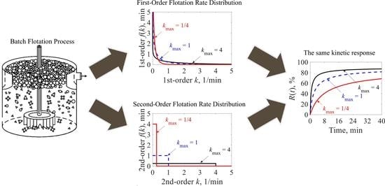
Four kinetic models are studied as first-order reactions with flotation rate distribution f(k): (i) deterministic nth-order reaction, (ii) second-order with Rectangular f(k), (iii) Rosin–Rammler, and (iv) Fractional kinetics. These models are studied because they are considered as alternatives to the first-order reactions. The first-order representation leads to the same recovery R(t) as in the original domain. The first-order R_∞-f(k) are obtained by inspection of the R(t) formulae or by inverse Laplace Transforms. The reaction orders of model (i) are related to the shape parameters of first-order Gamma f(k)s. Higher reaction orders imply rate concentrations at k ≈ 0 in the first-order domain. Model (ii) shows reverse J-shaped first-order f(k)s. Model (iii) under stretched exponentials presents mounded first-order f(k)s, whereas model (iv) with derivative orders lower than 1 shows from reverse J-shaped to mounded first-order f(k)s. Kinetic descriptions that lead to the same R(t) cannot be differentiated between each other. However, the first-order f(k)s can be studied in a comparable domain.

1. Introduction

1.1. Background

Kinetic models have been extensively used to study either the collection or the overall process (collection + separation) in flotation. The latter employs apparent rate constants to describe the recovery rates throughout the flotation process. The first kinetic studies reported in flotation were presented by Garcia-Zuñiga [1] and Schuhmann Jr [2], which described the respective processes by deterministic first-order rate constants k. The former also included a maximum achievable recovery R_∞ in the representation. From these pioneering works, any empirical deviation from the deterministic first-order approach has motivated alternative models to describe flotation kinetics [3,4,5,6,7].

Distributed first-order models have been widely used for kinetic characterizations and process modelling. Thus, empirical deviations regarding the first-order reaction with a deterministic rate constant have been attributed to a flotation rate distribution f(k), which incorporates all the heterogeneous conditions in the flotation process. The theoretical work reported by Sutherland [8] evaluated distributed internal variables in flotation and their effect on the recovery rates and process performances. Imaizumi and Inoue [5] and Woodburn and Loveday [9] extended the first-order models of Garcia-Zuñiga [1] and Schuhmann Jr [2] as continuous sum of exponentials to account for the wide range of recovery rates typically observed in flotation. The representation of the flotation process as a sum of rate constants has received more attention as the different flotation performances by size [10,11,12,13], by association [5,14], by liberation or composition [14,15,16,17] and others can be masked by a single probability density function. From the first-order generalizations reported by Imaizumi and Inoue [5] and Woodburn and Loveday [9] several distributions have been proposed to describe f(k), including Rectangular [18], Exponential (also named fully mixed reactor model) [19], Sinusoidal [20], Triangular [21], Normal [22], Double Normal [23] and Weibull [24], among others. The locations and shapes of these distributions define the predicted kinetic responses, which are a function of the relative presence of fast- and slow-floating components in the process.

Higher reaction orders have been reported in literature to explain differences regarding the deterministic first-order kinetics. For example, Arbiter [3] proposed the use of a second-order approach to represent six independent datasets. The recovery rate dependence (relative or fractional) on the initial mineral concentration was highlighted as evidence supporting the higher order assumption. Klimpel [25] extended the second-order model proposed by Arbiter [3] to describe batch flotation kinetics as second order reactions with Rectangular distribution of rate constants. Both approaches have been included when comparing different kinetic models to represent batch flotation processes [19,26,27,28,29,30,31,32,33,34]. Alternative reaction orders have also been investigated in literature [7,29,35,36,37]. de Bruyn and Modi [38] reported an empirical relationship between the flotation rate and the reaction order n for quartz at different particle sizes, assuming R_∞ = 100%. Continuous flotation tests were conducted on pure mineral, which led to a reaction order of approximately n = 1 for the size classes −65 µm and increasing n values in the +65 µm fractions. Holland-Batt [39] studied efficiency criteria for binary systems to assess batch flotation tests. Arbitrary reaction orders were considered, and R_∞ values of 100% were assumed for the two evaluated components (valuable and gangue). Brożek and Młynarczykowska [37] analysed kinetic models in batch flotation by comparison of nth-order reactions with an adsorption model derived from a first-order derivative equation. No froth effects were incorporated in the phenomenological model. More erratic responses at higher reaction orders were directly illustrated from the mathematical expressions. From size-by-size experimental data, the flotation responses were considered approximately homogeneous. Bu, Xie, Chen and Ni [27] studied the relationship between particle size and the reaction orders of the kinetic responses, which were found in the range n = 1–2. A maximum for n was obtained in the intermediate-coarse size class, which was attributed to the typical concave relationship between the flotation performance and particle size.

Other model structures have been used to describe flotation kinetics that cannot be categorized into the first- or nth-order reactions. For example, the Rosin–Rammler model has been proposed as an empirical approach to characterize kinetic responses in batch flotation [6,35,40,41]. However, the recovery mechanisms explained by the model parameters have not been explained in literature to date. Fractional calculus was also presented by Vinnett, et al. [42] as an alternative to characterize batch flotation kinetics. This approach has shown to be advantageous in anomalous systems with nonlocal dynamics that can be described by long-term memory in time [43]. From model fitting, Vinnett, Alvarez-Silva, Jaques, Hinojosa and Yianatos [42] showed that the Fractional derivatives were correlated with the shape parameters of the first-order Gamma model. Alvarez-Silva, et al. [44] obtained derivative orders greater than one, showing that the flexibility of Fractional kinetics can lead to unrealistic results in flotation (e.g., overshoots in the modelled R(t)).

As discussed in the previous two paragraphs, various model structures have been proposed as alternatives to the first-order reactions in flotation. However, special attention must be paid when the recovery expression R(t) can be also obtained from a first-order representation. For example, the second-order reaction with deterministic rate constant proposed by Arbiter [3] leads to the same algebraical formula as the first-order reaction with Exponential f(k). This match has been previously reported in literature based on the mathematical relationship between the R(t) formulae or on the estimated parameters and goodness-of-fit [19,29,32,35,45]. However, both models have been redundantly included in several comparisons and discussions on kinetic models in flotation [19,26,28,29,30,31,32,46,47,48,49,50,51,52,53,54,55,56]. Thus, for a combination of model parameters, the same R(t) can be obtained, implying that these two kinetic descriptions cannot be differentiated between each other.

The objective of this study is to obtain first-order representations for kinetic models that have been proposed as alternatives to the first-order reactions in batch flotation. These first-order representations consist of first-order R_∞-f(k) pairs that led to the same R(t) expression to that in the original domain (e.g., nth-order reaction, Rosin–Rammler model, Fractional kinetics). The first-order R_∞-f(k) pairs are obtained from the inversion of the continuous sum of exponentials reported by Imaizumi and Inoue [5] or by simple inspection of the R(t) expressions. The flotation rates can then be studied in a normalized domain, from which the presence of fast- (k >> 0) and slow-floating (k → 0) components can be identified. The fast- and slow-floating fractions are associated with the location and shapes of the first-order f(k)s, which are a function of the model parameters. The latter have been scarcely discussed in flotation literature except for the average rate constants. Thus, the model parameters of the alternative kinetic models can be related to a distribution of rate constants in the first-order domain.

1.2. Kinetic Models in Flotation

Kinetic models have typically considered the analogy with homogeneous chemical reactions. The flotation process is then represented as a reaction between particles and bubbles in excess [57,58,59,60]. Equation (1) expresses the rate of change of the instantaneous mineral concentration C in a batch flotation machine:

$$\frac{dC}{dt}=-k\cdot {\left(C-C_{\infty }\right)}^n$$

(1)

where C_∞ is the equilibrium concentration at t → ∞, n the reaction order and k the flotation rate constant.

1.2.1. First-Order Models

The special case with n = 1 (first-order model) was originally reported by Garcia-Zuñiga [1], which solved Equation (1) for the recovery as a function of time R(t):

$$R\left(t\right)=R_{\infty }\cdot \left[1-e^{{-k}_1\cdot t}\right]$$

(2)

Within Equation (2), k₁ corresponds to the first-order rate constant (deterministic) and R_∞ to the maximum achievable recovery at t → ∞.

Imaizumi and Inoue [5] extended the first-order model of Equation (2) to account for the wide range of recovery rates commonly observed in flotation. A flotation rate distribution f(k) was then proposed to represent the heterogeneous conditions in the separation process:

$$R\left(t\right)=R_{\infty }\cdot \left[1-{\displaystyle \underset{0}{\overset{\infty }{\int }}{e}^{-k\cdot t}f\left(k\right)dk}\right]$$

(3)

Different probability density functions (PDF) have been used in Equation (3) to represent f(k) and to obtain the respective R(t).

Table 1. Some flotation rate distributions and the respective recoveries in batch flotation processes.

Model	f(k)	R(t)
Single Rate Constant	${\delta }_{k_1}\left(k\right)$	$R_{\infty }\cdot \left[1-e^{-k_1\cdot t}\right]$
Rectangular	$\frac{1}{k_{\max }}\cdot \left[{\mu }_0\left(k\right)-{\mu }_{k_{\max }}\left(k\right)\right]$	$R_{\infty }\cdot \left[1-\frac{\left(1-e^{-k_{\max }\cdot t}\right)}{k_{\max }\cdot t}\right]$
Exponential	$\frac{1}{k_{\exp }}\cdot e^{-k/k_{\exp }}$	$R_{\infty }\cdot \left[1-\frac{1}{\left(1+k_{\exp }\cdot t\right)}\right]$
Gamma	$\frac{k^{a_G-1}}{k_G^{a_G}\cdot \Gamma \left(a_G\right)}\cdot e^{-k/k_G}$	$R_{\infty }\cdot \left[1-\frac{1}{{\left(1+k_G\cdot t\right)}^{a_G}}\right]$

(*) k₁ corresponds to the determinist rate constant in Equation (2), k_max to the maximum rate constant of a Rectangular f(k) with domain between 0 and k_max, k_exp to the mean rate constant of an Exponential distribution and a_G and k_G to the shape and scale parameters of a Gamma PDF. In addition, δ_x(k), μ_x(k) and Γ(x) denote the Dirac, Heaviside and Gamma functions, respectively.

shows examples of f(k)s commonly utilized to model first-order batch flotation, including Single Rate Constant, Rectangular, Exponential and Gamma models. The integral term of Equation (3) corresponds to the Laplace transform of f(k), with t = s. Therefore, f(k) can be obtained from the inverse Laplace transform of [1 − R(t = s)/R_∞]. This property has been used in literature to estimate f(k) from batch flotation data [61,62,63].

1.2.2. nth-Order Models

From Equation (1), any arbitrary reaction order can be studied. Equation (4) presents the recovery of a batch flotation process governed by a second-order reaction with deterministic rate constant k₂ [3]:

$$R\left(t\right)=\frac{R_{\infty }^2\cdot k_2\cdot t}{1+R_{\infty }\cdot k_2\cdot t}$$

(4)

Any reaction order can be generalized by a distribution of rate constants. Thus, Klimpel [25] presented Equation (5) as an extension of Equation (4), to describe batch flotation kinetics as second order reactions with Rectangular f(k):

$$R\left(t\right)=R_{\infty }\cdot \left[1-\frac{\ln \left(1+k_{\max }\cdot t\right)}{k_{\max }\cdot t}\right]$$

(5)

The solution of Equation (1) for an arbitrary reaction order n is given by Equation (6):

$$R\left(t\right)=R_{\infty }\cdot \left[1-\frac{1}{{\left(1+\left(n-1\right)\cdot R_{\infty }^{n-1}\cdot k_n\cdot t\right)}^{1/\left(n-1\right)}}\right]$$

(6)

Equation (6) represents a batch flotation process with a deterministic rate constant k_n in the nth-order domain. It should be mentioned that Equation (4) is a special case of Equation (6) with n = 2.

1.2.3. Other Model Structures

Alternative model structures to the first- and nth-order reactions have been also proposed to fit batch flotation kinetics. These models are empirical or represent different mechanisms to those explained by Equation (1).

The Rosin-Rammler model of Equation (7) is an empirical representation that has been reported in literature to characterize kinetic responses [6]:

$$R\left(t\right)=R_{\infty }\cdot \left[1-\exp \left(-{\left(k_{RR}\cdot t\right)}^{a_{RR}}\right)\right]$$

(7)

where k_RR and a_RR have been used as fitting parameters. The physical meaning of k_RR and a_RR has not been clearly established in flotation rate characterizations. However, k_RR can be interpreted as a decay rate constant whose reciprocal represents the time at which R(t) equals 63.21% of R_∞.

Fractional calculus has been proposed to represent anomalous kinetics with arbitrary derivative orders α [42]. Anomalous kinetics can be obtained from Equation (8):

$$\frac{d^{\alpha }C}{d{t}^{\alpha }}=-k_{\alpha }\cdot \left(C-C_{\infty }\right)$$

(8)

where k_α corresponds to the Fractional rate constant (time^−α). Non-integer derivative orders can then be used to model batch flotation kinetics. The recovery as a function of time is then given by Equation (9):

$$R\left(t\right)=R_{\infty }\cdot \left[1-E_{\alpha }\left(-k_{\alpha }\cdot t^{\alpha }\right)\right],E_{\alpha }\left(z\right)={\displaystyle \sum _{i=0}^{\infty }\frac{z^i}{\Gamma \left(\alpha \cdot i+1\right)}}$$

(9)

Within Equation (9), E_α(z) is the Mittag–Leffler function.

Models of Equations (5), (6), (7) and (9) are represented by first-order R_∞-f(k) pairs in Section 3 from the inversion of Equation (3) or from direct comparisons. These four models were chosen because they have been proposed as alternatives to the first-order reactions, showing specific flexibility to describe batch flotation data. The shapes of the first-order f(k)s are then analysed in terms of the different fast and slow-rate fractions in the first-order representation.

2. Materials and Methods

2.1. First-Order Representation

The nth-order reaction with deterministic rate constants, the second order reaction with Rectangular f(k), the Rosin–Rammler model, and the Fractional kinetics were studied as first-order reactions. First-order reactions with flotation rate distribution f(k)s that lead to the same R(t) expressions of Equations (5), (6), (7) and (9) were then obtained. Two methods were used for this purpose. The first method is applicable to R(t) models that have a first-order representation in literature, but whose equivalence has not been discussed in flotation. The simple inspection of the compared R(t) formulae allowed the conditions under which the models match to be determined. For example,

Table 2. Example of algebraical equivalence for the second-order model with single rate constant k₂ and a first order model with Exponential f(k).

2nd-Order Model with Single Rate Constant k2	First-Order Model with Exponential f(k)
$R\left(t\right)=\frac{R_{\infty }^2\cdot k_2\cdot t}{1+R_{\infty }\cdot k_2\cdot t}$	$\frac{1}{k_{\exp }}\cdot e^{-k/k_{\exp }}\to R\left(t\right)=R_{\infty }\cdot \left[1-{\displaystyle {\int }_0^{\infty }{e}^{-k\cdot t}\cdot f\left(k\right)dk}\right]=\frac{R_{\infty }\cdot k_{\exp }\cdot t}{\left(1+k_{\exp }\cdot t\right)}$

shows the algebraical equivalence of the R(t) expressions from the second-order model with deterministic rate constant and the first-order model with Exponential f(k). By inspection, the R(t) models coincide for the same R_∞ and with k_exp = R_∞∙k₂. The same recovery can then be obtained from a second-order reaction with a single rate constant and from a first-order reaction with Exponential f(k). The latter involves a fraction of floatable material with rate constants approaching to k = 0.

The second method to obtain the same R(t) from a first-order reaction was applied to those models that do not have a known first-order representation from literature. In this case, the studied R(t) models are equated to Equation (3) to represent the system as a continuous sum of exponentials in the first-order domain. The first-order f(k)s can be obtained from Equation (10):

$$f\left(k\right)={ℒ}^{-1}\left[1-\frac{R\left(t=s\right)}{R_{\infty }}\right]$$

(10)

where $ℒ$⁻¹ denotes the inverse Laplace Transform operator. Thus, for the same R_∞ and given the f(k) found by Equation (10), the same R(t) expression from the original domain is obtained in the first-order representation. The solution of Equation (10) was found by (i) tables of Laplace transforms or analytical/numerical solutions for Equation (10) reported in literature and (ii) the Symbolic Math Toolbox 8.5 of Matlab (R2020a, The MathWorks Inc., Natick, MA, USA). The methodology reported by Valsa and Brančik [64] was also used to numerically estimate the inverse Laplace transform of [1 − R(t = s)/R_∞], allowing the f(k) solutions to be crosschecked.

In summary, the R_∞-f(k) pairs in the first-order domain were obtained by simple inspection or by applying Equation (10). These first-order R_∞-f(k) pairs led to the same R(t) to those in the original domain. For the R(t) models of Equations (5), (6), (7) and (9), the shapes of the first-order f(k)s were then discussed in terms of the relative content of slow-rate constants.

2.2. Flotation Tests

Size-by-size kinetic responses for the Pb-Cu rougher separation (at batch scale) from a complex ore were used to illustrate first-order representations. The Pb and Cu feed grades were 2.46 ± 0.16% and 0.94 ± 0.04%, respectively. The grinding time was set to obtain 65% passing 38 µm. The grinding product was transferred to a 1.3L Denver Cell, and water was added to obtain 30% solids by mass. Sodium metabisulfite was added at 1500 g/ton to depress pyrite. An aeration stage of 20 min at superficial gas rate J_G = 0.16 cm/s was conducted for pyrite oxidation. Constant values for pH (9.3), collector concentration (45 g/ton of AeroPhine 3418A), frother concentration (24 ppm of Methyl Isobutyl Carbinol), and J_G (0.55 cm/s) were finally established. The concentrates were taken at ⅓, 1, 4.5, 10, 16, 24 and 32 minutes of flotation time, obtaining overall Pb and Cu recoveries of 82.4 ± 0.04%% and 90.7 ± 0.30%, respectively. Four size classes were studied: −20 μm, +20/−38 μm, +38/−75 μm and +75/−150 μm. Only the size-by-size kinetic responses for Cu are presented here for illustration purposes. The size classes +20/−38 μm and +38/−75 μm were analysed for the composite class +20/−75 μm for better visualization. For further details on the experimental procedure, please refer to [65]. The model parameters were obtained by least-squares estimation.

3. Results

3.1. nth-Order Models with Deterministic Rate Constants Represented as First-Order Models with Gamma f(k)s

The nth-order model with deterministic rate constant k_n was compared to a first-order model with Gamma f(k).

Table 3. nth-order model with deterministic rate constant k_n versus.

nth-Order Model with Single Rate Constant kn	First-Order Model with Gamma f(k)
$R\left(t\right)=R_{\infty }\cdot \left[1-\frac{1}{{\left(1+\left(n-1\right)\cdot R_{\infty }^{n-1}\cdot k_n\cdot t\right)}^{1/\left(n-1\right)}}\right]$	$R\left(t\right)=R_{\infty }\cdot \left[1-\frac{1}{{\left(1+k_G\cdot t\right)}^{a_G}}\right]$

shows the R(t) expressions for these model structures. For further details about the parameters of the Gamma model, please refer to Table 1. A direct comparison between these models shows that both approaches are algebraically identical. Equation (11) shows the relationship between the model parameters (at the same R_∞) that guarantee the R(t) match. Thus, the sets (n, k_n) and (a_G, k_G) that satisfy Equation (11) lead to the same R(t) expression. This property has been previously studied in different areas of process and chemical engineering as a tool to estimate apparent reaction orders [66,67,68,69,70]. The deterministic parameters of the nth-order model can then be related to the Gamma f(k) shapes and locations in the first-order representation. It should be mentioned that the example of Table 2 is a special case of the R(t) models presented in Table 3 with n = 2 and a_G = 1, respectively.

$$k_n=\frac{k_G\cdot a_G}{\sqrt[a_G]{R_{\infty }}},n=1+\frac{1}{a_G}$$

(11)

Figure 1a shows three first-order Gamma f(k)s with the same average rate constant k_ave = k_G∙a_G = 1. The parameters of these Gamma PDFs were chosen because they represent reverse J-shaped (a_G < 1), Exponential (a_G = 1) and mound-shaped (a_G > 1) distributions in the first-order domain. The latter approaches to Normal distributions when a_G >> 1 and to deterministic rate constants when a_G → ∞ and k_G → k_ave/a_G. First-order systems with a high fraction of slow flotation rates can be obtained from Gamma PDFs with a_G ≤ 1. In the example of Figure 1a, a vertical asymptote is observed at k = 0 with a_G = 1/4. Figure 1b shows the time-recovery curves for first-order Gamma f(k)s under the k_G and a_G values depicted in Figure 1a. A maximum recovery of 90% was assumed. As shown in Figure 1b, much slower increasing trends are observed in the time-recovery curves for a_G ≤ 1 as t → ∞. The identification of this slow-rate constants makes it possible to determine the sensitivity of a floatable mineral to the total experimental time. The fraction of rate constants approaching to zero then defined the rate-limited losses in batch flotation. Figure 1c presents the n-th order (n = 1.06, 2 and 5) rate constants that lead to the same time-recovery curves of Figure 1b. The n and k_n values were obtained from Equation (11), given the k_G and a_G values presented in Figure 1a. Thus, the sustained increasing trends in the time recovery curves are observed from nth-order models with n ≥ 2. Therefore, higher reaction orders can be interpreted as more slow-floating components in the respective first-order system. Notice that the locations of k_n in Figure 1c are a function of R_∞, as shown in Equation (11).

Figure 2 shows the estimated first-order and nth-order f(k)s and model fitting for the size-by-size flotation tests. As expected, both representations led to the same R_∞ from the model fitting with rate parameters that satisfy Equation (11). The flexibility of the R(t) model of Table 3 was adequate to represent the experimental data, as shown in Figure 2b. The first-order f(k)s of Figure 2a showed a transition from a reverse J-shaped f(k) (a_G < 1) in the −20 µm class to a mounded f(k) (a_G > 1) in the +75/−150 µm class. The reverse J-shaped f(k) justified the sustained increasing recoveries in Figure 2b for the −20 µm class. The change in the first-order f(k) shapes is observed in the nth-order domain by a reaction order decrease towards the coarse class, as shown in Figure 2c.

3.2. Second-Order Model with Rectangular f(k) Represented as a Distributed First-Order Reaction

Klimpel [25] presented the second-order model with Rectangular distribution of rate constants [0-k_max] shown in

Table 4. Second-order model with Rectangular f(k) [0-k_max] versus its first-order representation.

Second-Order Model with Rectangular f(k) [0-kmax]	Distributed First-Order Model
$R\left(t\right)=R_{\infty }\cdot \left[1-\frac{\ln \left(1+k_{\max }\cdot t\right)}{k_{\max }\cdot t}\right]$	$R\left(t\right)=R_{\infty }\cdot \left[1-{\displaystyle {\int }_0^{\infty }{e}^{-k\cdot t}\cdot f\left(k\right)dk}\right]$

. No representations of this R(t) model from first-order f(k)s have been reported in flotation literature. The first- and second-order expressions of Table 4 were then equated to determine the respective first-order f(k). Equation (12) presents the solution for this first-order f(k), after applying the Inverse Laplace Transform to [1 − R(t = s)/R_∞].

$$f\left(k\right)={ℒ}^{-1}\left[\frac{\ln \left(1+k_{\max }\cdot s\right)}{k_{\max }\cdot s}\right]=\frac{1}{k_{\max }}{E}_1\left(\frac{k}{k_{\max }}\right)=\frac{1}{k_{\max }}{\displaystyle {\int }_{k/k_{\max }}^{\infty }\frac{e^{-x}}{x}dx}$$

(12)

The result of Equation (12) has been presented in different Laplace transform tables e.g., [71] and can also be obtained from the Symbolic Math Toolbox of Matlab (The MathWorks Inc., Natick, MA, USA). The integral term in Equation (12) corresponds to the exponential integral function E₁. Figure 3a shows three examples of the first-order f(k)s. The average rate constant of this f(k) is k_max/2. The same average is obtained from the second-order flotation rate distribution (Rectangular PDF). The k_max values were chosen to obtain comparable R(t) trends to those observed in Figure 1b. The first-order f(k)s corresponded to reverse J-shaped distributions in all cases, from which high fractions of slow-floating components are observed. As a result, Figure 3b shows sustained and slow increasing trends at long flotation times in the kinetic responses (R_∞ = 90%). Figure 3c shows the second-order f(k)s. A second-order model with a deterministic rate constant can be expressed as a first-order model with Exponential f(k), as illustrated in Table 2. This Exponential distribution has a moderate content of rate constants approaching to k = 0. Thus, distributed second-order reactions as those shown in Figure 3c lead to significantly higher fractions of slow flotation rates in the first-order representation. The second-order model with Rectangular f(k) led to time-recovery curves presenting sustained increasing trends as t → ∞, which is observed by an asymptote at k = 0 in the first-order f(k)s of Figure 3a. Flotation schemes that are adequately described by this model structure will be typically sensitive to the flotation time, with significant slow-rate losses at the end of the process. It should be mentioned that similar first-order f(k)s to those of Figure 3a can be obtained from Gamma PDFs with a_G < 1, as shown in Figure 1a.

Figure 4 presents the results obtained from the size-by-size experimental data. Except for the −20 µm class, the R(t) model of Table 4 showed poor performance to represent the time-recovery data (Figure 4b). As the −20 µm class presented sustained increasing recoveries at long flotation times, the R(t) model of Table 4 was adequate for this size class. Despite the k_max differences shown in Figure 4c in the second order domain, the first-order f(k)s were similar. This feature limits the flexibility of this model structure.

3.3. Rosin-Rammler Model Represented as a Distributed First-Order Model

The Rosin–Rammler R(t) model has also been reported in literature to characterize kinetic responses. Neither a flotation rate representation (e.g., an f(k) in any rate domain) nor the relationship of the model parameters with the fast- and slow-floating components have been reported in flotation. The Laplace inversion of [1 − R(t = s)/R_∞] was again used to represent this model from first-order f(k)s. Two conditions must be taken into consideration: (i) for a_RR ≤ 1, the argument of the Inverse Laplace transform $\left[\exp \left(-{\left(k_{RR}\cdot t\right)}^{a_{RR}}\right)\right]$ corresponds to a stretched exponential, which allows first-order f(k)s to be obtained from Equation (13) [72,73], (ii) for a_RR > 1, the argument of the Inverse Laplace transform corresponds to a compressed exponential, which cannot be represented by the sum of exponentials of

Table 5. Rosin–Rammler model versus its first-order representation.

Rosin-Rammler Model	Distributed First-Order Model
$R\left(t\right)=R_{\infty }\cdot \left[1-\exp \left(-{\left(k_{RR}\cdot t\right)}^{a_{RR}}\right)\right]$	$R\left(t\right)=R_{\infty }\cdot \left[1-{\displaystyle {\int }_0^{\infty }{e}^{-k\cdot t}\cdot f\left(k\right)dk}\right]$

[72]. Thus, the compressed exponentials cannot be represented by first- nor any nth-order reaction.

The Inverse Laplace transform of the stretched exponential (a_RR ≤ 1) was obtained from numerical integration of Equation (13). The first-order f(k)s were crosschecked from the numerical Laplace inversion of [1 − R(t = s)/R_∞], using the methodology reported by Valsa and Brančik [64]. The normalized tables reported by Dishon, et al. [74] were also used to support the results. In case of compressed exponentials (a_RR > 1), the Rosin–Rammler model suggests a decaying mechanism that is faster than any exponential function at long flotation times [72], which cannot be expressed by the distributed first-order model of Table 5.

$$\begin{array}{ll}{f\left(k\right)|}_{0\le a_{RR}\le 1}& ={ℒ}^{-1}\left[\exp \left(-{\left(k_{RR}\cdot s\right)}^{a_{RR}}\right)\right]\\ & =\frac{1}{\pi \cdot k_{RR}}{\displaystyle {\int }_0^{\infty }\exp \left[-u^{a_{RR}}\cdot \cos \left(\beta \right)\right]\cos \left[\frac{k}{k_{RR}}\cdot u-u^{a_{RR}}\cdot \sin \left(\beta \right)\right]du}\\ & \beta =\frac{\pi \cdot a_{RR}}{2}\end{array}$$

(13)

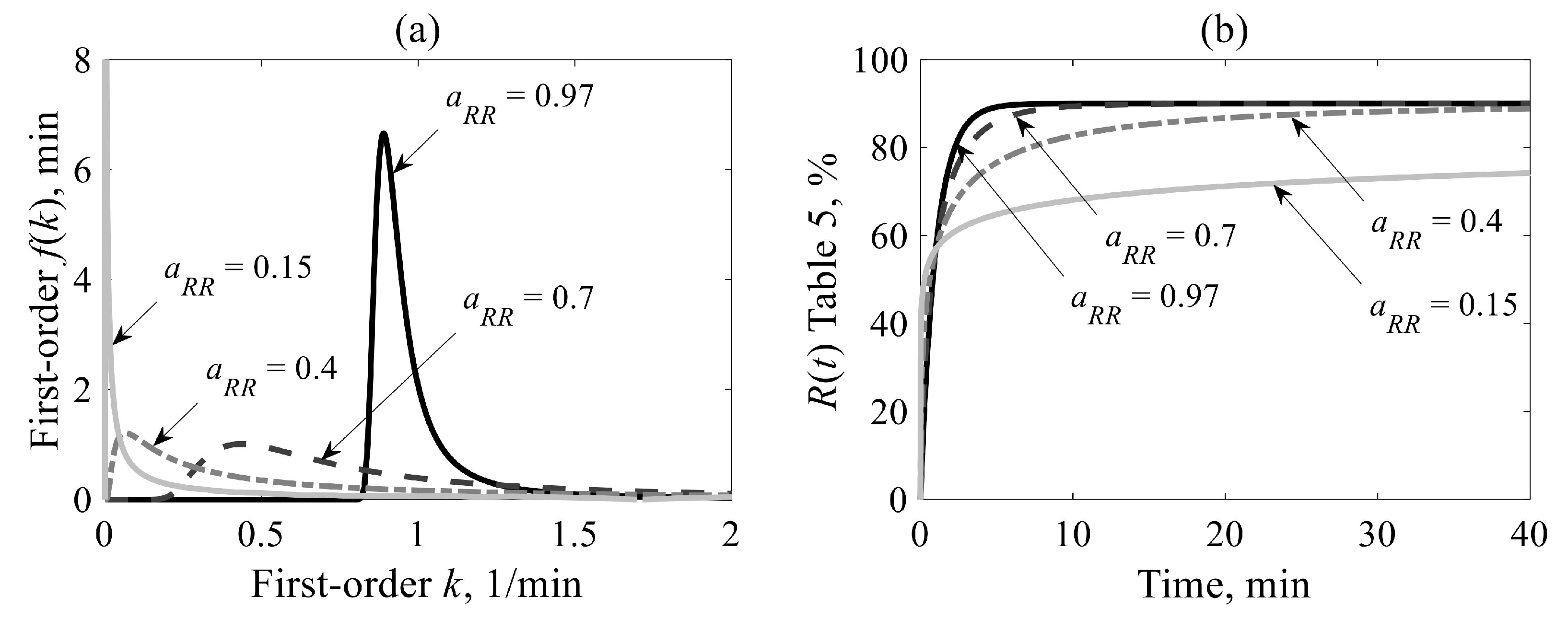
Figure 5 illustrates four first-order f(k)s from the Rosin-Rammler R(t) together with the respective time-recovery curves for a_RR < 1. No additional flotation rate descriptions have been reported in literature for this model. A maximum recovery of 90% was considered with k_RR = 1 min⁻¹. Different k_RR values will scale the domain and codomain of the flotation rate distributions. The a_RR values in Figure 5 were chosen to illustrate the presence of slow-floating components in the first-order f(k)s and their convergence to deterministic rate constants. For a_RR → 0, the equivalent first-order f(k)s present a high fraction of slow flotation rates. However, the solutions of Equation (13) are also long-tailed distributions [75], with a significant fraction of fast flotation rates and then with dR/dt → ∞ as t → 0. Thus, sustained increasing trends in the time-recovery curves were observed at low a_RR values, but with a very fast recovery rates at the beginning of the processes. As a_RR increased, mounded-shaped distributions were obtained. For a_RR ≈ 1, the equivalent f(k) converged to a first-order model with a deterministic rate constant. The condition with a_RR = 0.97 exemplifies this convergence. The average rate constant is infinite for 0 < a_RR < 1 [76]; therefore, the flotation rate distribution cannot be described by this location parameter. From the results of Figure 5, the Rosin-Rammler model can describe rate-limited processes with a_RR → 0, which leads to sustained increasing trends in the time-recovery curves. For a_RR > 0.5 and k_RR = 1, the slow-floating components are negligible as shown in Figure 5a, resulting in time recovery curves that reached a plateau at 10 min of flotation.

Ahmed [6] and Sahoo, Suresh and Varma [40] reported a_RR values greater than 1, which corresponded to the compressed exponential decay. For a_RR ≥ 1, dR/dt = 0 at t = 0, which can be only justified by a delay in the flotation process. Initially, the compressed exponential case presents increasing instantaneous recovery rates up to a maximum is reached. Thereafter, a fast decreasing trend is typically obtained. This feature may be adequate to model the kinetic response of some components subject to delayed separation in batch flotation. For example, slow-floating particles that are recovered after most of the easy-to-float components have been recovered.

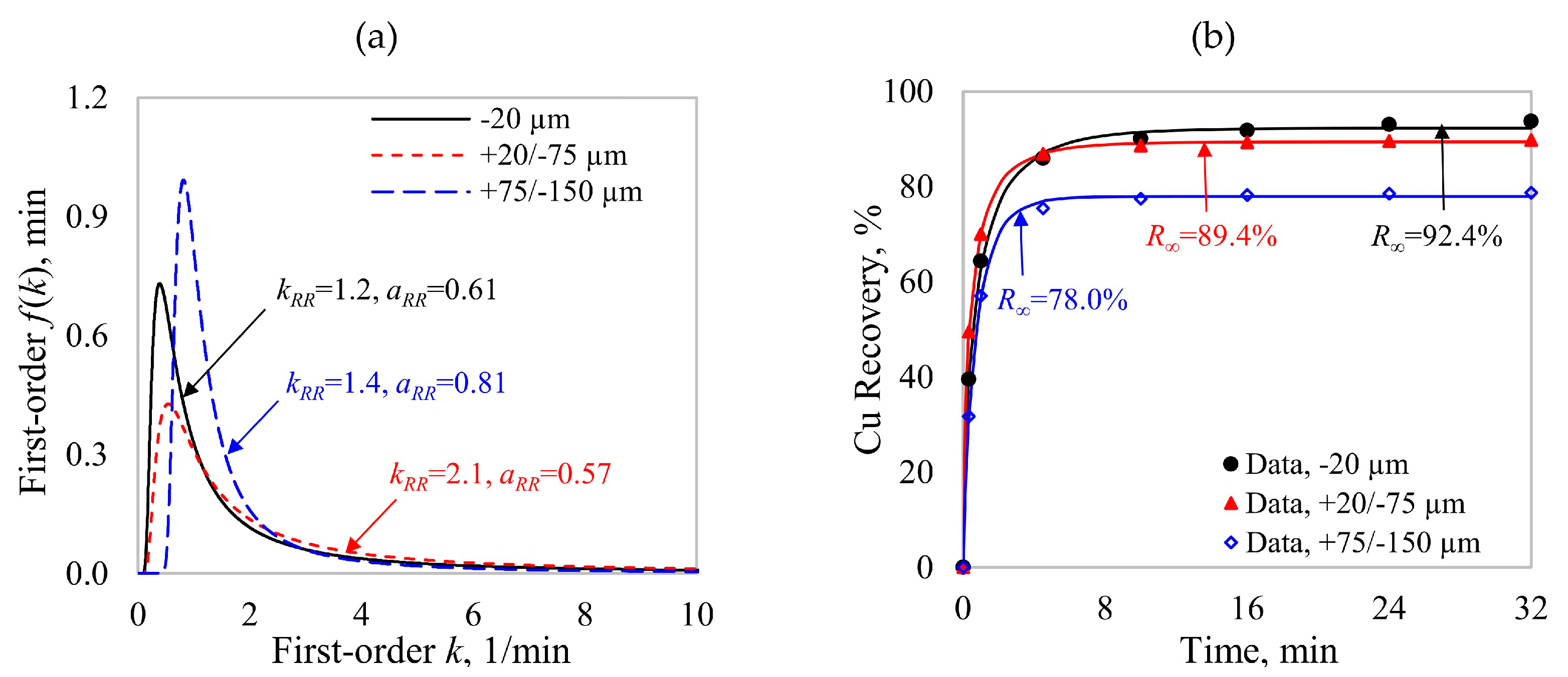
Figure 6 shows the estimated first-order f(k)s and model fitting for the size-by-size tests. No compressed exponentials were obtained from the experimental data. Only the +20/−75 µm class was adequately described by the Rosin-Rammler model of Table 5. Although this model structure was not suitable to describe the kinetic responses in the fine and coarse classes, the first-order f(k)s presented some features observed in Figure 2a from Gamma f(k)s. For example, the −20 µm size class tended to concentrate to slower rate constants as shown in Figure 6a. The +75/−150 µm class approached a deterministic rate constant, which was also observed as a Gamma f(k) with a_G ≈ 2.1.

3.4. Fractional Kinetics as Distributed First-Order Reactions

Fractional calculus has been also presented as an alternative to the first- and nth-order models to characterize batch flotation kinetics.

Table 6. Fractional kinetics versus its first-order representation.

Fractional Kinetics	Distributed First-Order Model
$R\left(t\right)=R_{\infty }\cdot \left[1-E_{\alpha }\left(-k_{\alpha }\cdot t^{\alpha }\right)\right]$	$R\left(t\right)=R_{\infty }\cdot \left[1-{\displaystyle {\int }_0^{\infty }{e}^{-k\cdot t}\cdot f\left(k\right)dk}\right]$

shows the Fractional R(t). No first-order representation for this model has been discussed in flotation literature to date. The Fractional kinetics of Table 6 was then studied from the first-order f(k)s. For a derivative order 0 < α < 1, this first-order f(k) was again obtained from the Inverse Laplace transform of the Mittag–Leffler function, as expressed by Equation (14) [77]. For α > 1, E_α presents oscillations around zero and then overshoots in the time-recovery curves. This feature does not have a physical meaning in flotation as previously observed by Alvarez-Silva, Vinnett, Langlois and Waters [44]. The f(k) results were again crosschecked by the Inversion methodology presented by Valsa and Brančik [64].

$${f\left(k\right)|}_{0\le \alpha \le 1}={ℒ}^{-1}\left[E_{\alpha }\left(-k_{\alpha }\cdot s^{\alpha }\right)\right]=\frac{1}{\pi }\cdot \left[\frac{k_{\alpha }\cdot k^{\alpha -1}\cdot \sin \left(\alpha \cdot \pi \right)}{k^{2\cdot \alpha }+2\cdot k_{\alpha }\cdot k^{\alpha }\cdot \cos \left(\alpha \cdot \pi \right)+k_{\alpha }^2}\right]$$

(14)

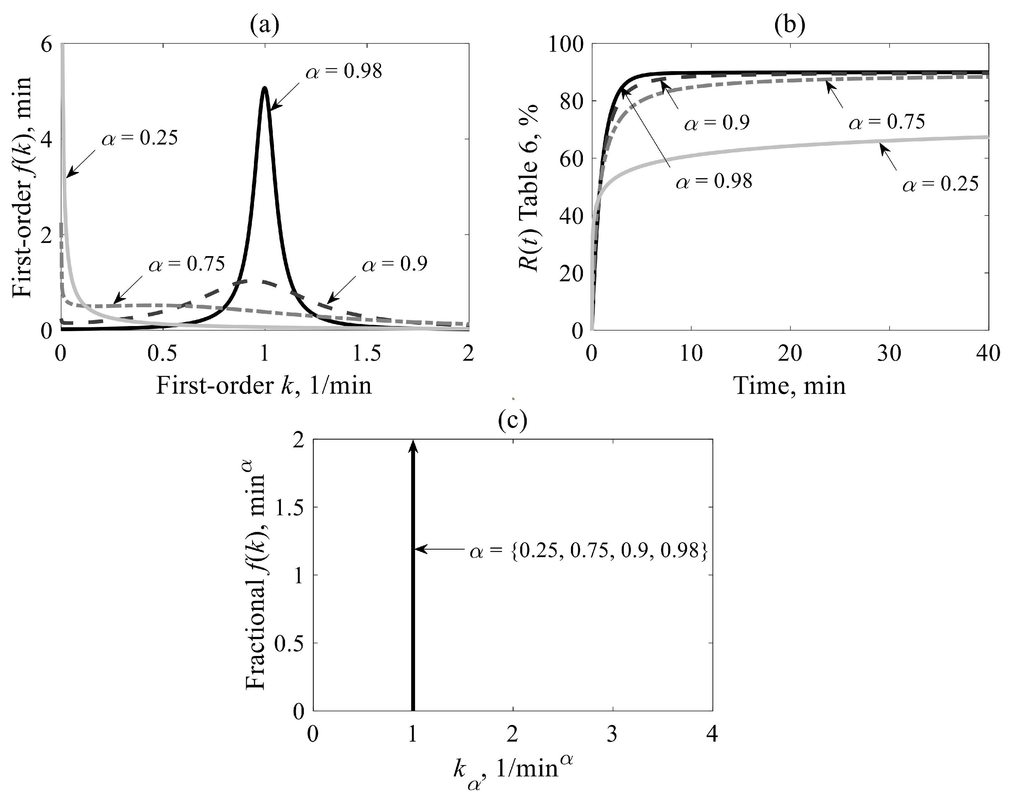
Figure 7a shows four first-order f(k)s obtained from different derivative orders in the Fractional approach, assuming k_α = 1 min^−α and R_∞ = 90 %. The derivative orders were selected to present from reverse J-shaped f(k)s to approximately deterministic rate constants in the first-order domain. The time-recovery curves are also presented in Figure 7b. For low α values, reverse J-shaped distributions are obtained, which gradually change to mounded PDFs as the derivative order increases. However, a concentration of rate constants is observed close to k = 0 even for moderate-high α values. Long tails are then obtained to compensate the asymptotic behaviour at k = 0. For α ≈ 1, the first-order f(k) approached to a deterministic rate constant. As with the Rosin-Rammler model, the first-order f(k) cannot be characterized by a mean rate constant. The kinetics responses of Figure 7b showed similar patterns as those obtained with the Rosin-Rammler model under stretched exponentials, with very fast recovery rates at t = 0. Conditions with α = 0.25 and α = 0.75 presented an asymptote at k = 0 as shown in Figure 7a, which led to sustained increasing recoveries in Figure 7b. Flotation processes described by these conditions are subject to slow-rate losses and requires longer flotation times to obtain the steady recoveries defined by R_∞. Figure 7c shows the deterministic rate constants in the Fractional domain (k_α = 1 min^−α), which indicate that the changes in the kinetic responses were associated to the different derivative orders in the proposed example [α = 0.25, 0.75, 0.9, 0.98].

Figure 8 details the results from the size-by-size experimental data. The flexibility of the Fractional model was comparable to that of the R(t) model of Table 3 (see Figure 2). The first-order f(k)s of Figure 8a presented higher content of rate constants close to zero in the finer classes, whereas a more deterministic distribution was observed in the +75/−150 µm class. The concentration of k ≈ 0 favored the sustained increasing trends in the R(t) models. More deterministic first-order f(k)s are represented in the Fractional domain by a derivative order that is closer to 1.

4. Discussion

Several model structures for R(t) have been proposed in literature as alternatives to the first-order reactions in batch flotation (e.g., nth-order reactions with continuous or discrete f(k), Rosin–Rammler R(t), Fractional kinetics). The results of Figure 1, Figure 2, Figure 3, Figure 4, Figure 5, Figure 6, Figure 7 and Figure 8 showed that the four evaluated models can be represented as first-order reactions with flotation rate distributions f(k)s. From the studied models, only the Rosin–Rammler approach with compressed exponentials (a_RR > 1) cannot be explained from first-order mechanisms. Thus, any kinetic model with a process decay representable as a sum of exponentials (continuous or discrete) has a first-order R_∞-f(k) pair. This feature implies that two kinetic descriptions that lead to the same R(t) cannot be differentiated empirically between each other. However, the first-order representation allows for f(k) comparisons in a normalized rate domain. In addition, the locations and shapes of these first-order flotation rate distributions are directly related to the R(t) responses as shown in Figure 1, Figure 2, Figure 3, Figure 4, Figure 5, Figure 6, Figure 7 and Figure 8. These locations and shapes are a function of the model parameters, which have been used to fit experimental data but scarcely related to the flotation responses. The flexibility of Equations (5), (6), (7) and (9) can then be associated with the presence of slow- and fast-floating fractions, which affect the kinetic responses at short and long flotation times. From the results reported here, only R(t) models with decays that are faster than any exponential function can justify flotation mechanisms not representable in the first-order domain.

5. Conclusions

Four kinetic models were studied as first-order systems with flotation rate distributions f(k)s. These models were analysed because they have been presented as alternatives to the first-order reactions in batch flotation. The first-order representations were obtained from direct comparisons between the R(t) expressions or from the inverse Laplace transform of [1 − R(t = s)/R_∞]. Thus, the compared approaches led to the same algebraical R(t)s. The results indicated that:

• The nth-order reactions with determinist rate constants can be represented as first-order reactions with Gamma f(k)s. Low reaction orders indicate approximately deterministic rate constants, whereas high reaction orders indicate J-shaped f(k)s. The latter implies a high presence of slow-floating components (k → 0).
• The second-order reaction with Rectangular distribution of rate constants can be represented as a first-order reaction with f(k) = 1/k_max∙E₁(k/k_max). These first-order f(k)s are always reverse J-shaped distributions, indicating high concentrations of slow rate constants and then sustained increasing trends in R(t).
• The Rosin–Rammler model has a first-order representation for a_RR ≤ 1 (stretched exponentials). In this case, the typically unimodal f(k)s only presented rate constants close to zero with a_RR → 0. For a_RR > 1 (compressed exponentials), the Rosin–Rammler model does not have a first-order representation.
• The Fractional kinetics can be represented as a first-order reaction for α ≤ 1. Although the f(k)s approached to deterministic rate constants as α → 1, slow rate fractions were observed up to moderate high α values. For α > 1, the Fractional approach does not have physical meaning in flotation.

The first-order representation allows the f(k) shapes and the fast- and slow-floating components to be qualitatively or quantitatively studied in a normalized k domain. Only conditions with a decay that is faster than any exponential function (e.g., compressed exponentials) can be considered as alternatives to the first-order reactions in batch flotation.

References

- Garcia-Zuñiga, H. La recuperación por flotación es una función exponencial del tiempo. Boletín Minero, Sociedad Nacional de Minería 1935, 47, 83–86. [Google Scholar]
- Schuhmann, R., Jr. Flotation Kinetics. I. Methods for steady-state study of flotation problems. J. Phys. Chem. 1942, 46, 891–902. [Google Scholar] [CrossRef]
- Arbiter, N. Flotation rates and flotation efficiency. Trans. Am. Inst. Min. Metall. Eng. 1951, 190, 791–796. [Google Scholar]
- Kelsall, D.F. Application of probability assessment of flotation systems. Trans. Inst. Min. Metall. 1961, 70, 191–204. [Google Scholar]
- Imaizumi, T.; Inoue, T. Kinetic consideration of froth flotation. In Proceedings of the Sixth International Mineral Processing Congress, Cannes, France, 26 May–2 June 1963; pp. 581–593. [Google Scholar]
- Ahmed, M.M. Discrimination of different models in the flotation of Maghara coal. Miner. Process. Extr. Metall. 2004, 113, 103–110. [Google Scholar] [CrossRef]
- Horst, W. Scale-up relationships in spodumene flotation. Min. Eng. 1958, 10, 1182–1185. [Google Scholar]
- Sutherland, K.L. Physical chemistry of flotation. XI. Kinetics of the flotation process. J. Phys. Chem. 1948, 52, 394–425. [Google Scholar] [CrossRef]
- Woodburn, E.T.; Loveday, B.K. The effect of variable residence time on the performance of a flotation system. J. S. Afr. Inst. Min. Metall. 1965, 65, 612–628. [Google Scholar]
- Trahar, W.J. A rational interpretation of the role of particle size in flotation. Int. J. Miner. Process. 1981, 8, 289–327. [Google Scholar] [CrossRef]
- Morris, T. Measurement and evaluation of the rate of flotation as a function of particle size. Min. Eng. 1952, 4, 794–798. [Google Scholar]
- Gaudin, A.M.; Groh, J.O.; Henderson, H.B. Effect of particle size on flotation. Am. Inst. Min. Metall. Eng. 1931, 414, 3–23. [Google Scholar]
- Gaudin, A.M.; Schuhmann, R., Jr.; Schlechten, A.W. Flotation Kinetics. II. The Effect of Size on the Behavior of Galena Particles. J. Phys. Chem. 1942, 46, 902–910. [Google Scholar] [CrossRef]
- Sutherland, D.N. Batch flotation behaviour of composite particles. Miner. Eng. 1989, 2, 351–367. [Google Scholar] [CrossRef]
- Bartlett, D.R.; Mular, A.L. Dependence of flotation rate on particle size and fractional mineral content. Int. J. Miner. Process. 1974, 1, 277–286. [Google Scholar] [CrossRef]
- Welsby, S.D.D.; Vianna, S.M.S.M.; Franzidis, J.-P. Assigning physical significance to floatability components. Int. J. Miner. Process. 2010, 97, 59–67. [Google Scholar] [CrossRef]
- Jameson, G.J. The effect of surface liberation and particle size on flotation rate constants. Miner. Eng. 2012, 36–38, 132–137. [Google Scholar] [CrossRef]
- Huber-Panu, I.; Ene-Danalache, E.; Cojocariu, D.G. Mathematical models of batch and continuous flotation. In Flotation—A. M. Gaudin Memorial; American Institute of Mining, Metallurgical, and Petroleum Engineers, Inc.: New York, NY, USA, 1976; Volume 2, pp. 675–724. [Google Scholar]
- Dowling, E.C.; Klimpel, R.R.; Aplan, F.F. Model discrimination in the flotation of a porphyry copper ore. Miner. Metall. Process. 1985, 2, 87–101. [Google Scholar] [CrossRef]
- Diao, J.; Fuerstenau, D.; Hanson, J. Kinetics of coal flotation. In Proceedings of the SME-AIME Annual Meeting, Phoenix, AZ, USA, 21–24 February 2016. [Google Scholar]
- Harris, C.; Chakravarti, A. Semi-batch froth flotation kinetics: Species distribution analysis. Trans. AIME 1970, 247, 162–172. [Google Scholar]
- Chander, S.; Polat, M. Flotation Kinetics: Methods for Estimating Distribution of Rate Constants. In Proceedings of the International Mineral Processing Congress (XIX IMPC), San Francisco, CA, USA, 22–27 October 1995; pp. 105–111. [Google Scholar]
- Ferreira, J.P.; Loveday, B.K. An improved model for simulation of flotation circuits. Miner. Eng. 2000, 13, 1441–1453. [Google Scholar] [CrossRef]
- Yianatos, J.; Bergh, L.; Vinnett, L.; Contreras, F.; Díaz, F. Flotation rate distribution in the collection zone of industrial cells. Miner. Eng. 2010, 23, 1030–1035. [Google Scholar] [CrossRef]
- Klimpel, R.R. Selection of chemical reagents for flotation. In Mineral Processing Plant Design; Mular, A.L., Bhappu, R.B., Eds.; SME-AIME: New York, NY, USA, 1980; Volume 2, pp. 907–934. [Google Scholar]
- Bahrami, A.; Ghorbani, Y.; Hosseini, M.R.; Kazemi, F.; Abdollahi, M.; Danesh, A. Combined Effect of Operating Parameters on Separation Efficiency and Kinetics of Copper Flotation. Min. Metall. Explor. 2019, 36, 409–421. [Google Scholar] [CrossRef] [Green Version]
- Bu, X.; Xie, G.; Chen, Y.; Ni, C. The Order of Kinetic Models in Coal Fines Flotation. Int. J. Coal Prep. Util. 2017, 37, 113–123. [Google Scholar] [CrossRef]
- Chaves, A.P.; Ruiz, A.S. Considerations on the Kinetics of Froth Flotation of Ultrafine Coal Contained in Tailings. Int. J. Coal Prep. Util. 2009, 29, 289–297. [Google Scholar] [CrossRef]
- Ek, C. Flotation Kinetics. In Innovations in Flotation Technology; Mavros, P., Matis, K.A., Eds.; Springer: Dordrecht, The Netherlands, 1992; pp. 183–210. [Google Scholar]
- Ni, C.; Xie, G.; Jin, M.; Peng, Y.; Xia, W. The difference in flotation kinetics of various size fractions of bituminous coal between rougher and cleaner flotation processes. Powder Technol. 2016, 292, 210–216. [Google Scholar] [CrossRef]
- Yuan, X.M.; Palsson, B.I.; Forssberg, K.S.E. Statistical interpretation of flotation kinetics for a complex sulphide ore. Miner. Eng. 1996, 9, 429–442. [Google Scholar] [CrossRef]
- Zhang, H.; Liu, J.; Cao, Y.; Wang, Y. Effects of particle size on lignite reverse flotation kinetics in the presence of sodium chloride. Powder Technol. 2013, 246, 658–663. [Google Scholar] [CrossRef]
- Yang, X.; Huang, X.; Qiu, T. Activation-flotation kinetics of depressed marmatite and chalcopyrite in cyanidation tailings using sodium hypochlorite as activator. Miner. Metall. Process. 2016, 33, 131–136. [Google Scholar] [CrossRef]
- Tijsseling, L.T.; Dehaine, Q.; Rollinson, G.K.; Glass, H.J. Mineralogical Prediction of Flotation Performance for a Sediment-Hosted Copper–Cobalt Sulphide Ore. Minerals 2020, 10, 474. [Google Scholar] [CrossRef]
- Bu, X.; Xie, G.; Peng, Y.; Ge, L.; Ni, C. Kinetics of flotation. Order of process, rate constant distribution and ultimate recovery. Physicochem. Probl. Miner. Process. 2017, 53, 342–365. [Google Scholar]
- Tewari, S.N.; Biswas, A.K. Flotation kinetics for calcite in a semi-batch system. J. Appl. Chem. 1969, 19, 173–177. [Google Scholar] [CrossRef]
- Brożek, M.; Młynarczykowska, A. Analysis of kinetics models of batch flotation. Physicochem. Probl. Miner. Process. 2007, 41, 51–65. [Google Scholar]
- de Bruyn, P.L.; Modi, H.J. Particle Size and Flotation Rate of Quartz. Am. Inst. Min. Metall. Pet. Eng. 1956, 205, 415–419. [Google Scholar]
- Holland-Batt, A.B. Efficiency in batch separations. Inst. Mater. Miner. Min. 1971, 80, C12–C23. [Google Scholar]
- Sahoo, S.K.; Suresh, N.; Varma, A.K. Performance Evaluation of Basic Flotation Kinetic Models Using Advanced Statistical Techniques. Int. J. Coal Prep. Util. 2019, 39, 65–87. [Google Scholar] [CrossRef]
- Sokolovic, J.; Miskovic, S. The effect of particle size on coal flotation kinetics: A review. Physicochem. Probl. Miner. Process. 2018, 54, 1172–1190. [Google Scholar]
- Vinnett, L.; Alvarez-Silva, M.; Jaques, A.; Hinojosa, F.; Yianatos, J. Batch flotation kinetics: Fractional calculus approach. Miner. Eng. 2015, 77, 167–171. [Google Scholar] [CrossRef]
- Tarasov, V.E. Fractional Dynamics: Applications of Fractional Calculus to Dynamics of Particles, Fields and Media; Springer Science & Business Media: Berlin/Heidelberg, Germany, 2011. [Google Scholar]
- Alvarez-Silva, M.; Vinnett, L.; Langlois, R.; Waters, K.E. A comparison of the predictability of batch flotation kinetic models. Miner. Eng. 2016, 99, 142–150. [Google Scholar] [CrossRef]
- Zhang, X.; Han, Y.; Gao, P.; Li, Y.; Sun, Y. Effects of particle size and ferric hydroxo complex produced by different grinding media on the flotation kinetics of pyrite. Powder Technol. 2020, 360, 1028–1036. [Google Scholar] [CrossRef]
- Hassanzadeh, A.; Hoang, D.H.; Brockmann, M. Assessment of flotation kinetics modeling using information criteria; case studies of elevated-pyritic copper sulfide and high-grade carbonaceous sedimentary apatite ores. J. Dispers. Sci. Technol. 2020, 41, 1083–1094. [Google Scholar] [CrossRef]
- Liao, Y.; Cao, Y.; Liu, C.; Zhu, G. A Study of Kinetics on Oily-Bubble Flotation for a Low-Rank Coal. Int. J. Coal Prep. Util. 2016, 36, 151–162. [Google Scholar] [CrossRef]
- Bu, X.; Xie, G.; Peng, Y.; Chen, Y. Kinetic modeling and optimization of flotation process in a cyclonic microbubble flotation column using composite central design methodology. Int. J. Miner. Process. 2016, 157, 175–183. [Google Scholar] [CrossRef]
- Ma, G.; Xia, W.; Xie, G. Effect of particle shape on the flotation kinetics of fine coking coal. J. Clean. Prod. 2018, 195, 470–475. [Google Scholar] [CrossRef]
- Mao, Y.; Bu, X.; Peng, Y.; Tian, F.; Xie, G. Effects of simultaneous ultrasonic treatment on the separation selectivity and flotation kinetics of high-ash lignite. Fuel 2020, 259, 116270. [Google Scholar] [CrossRef]
- Chen, S.; Tao, X.; Wang, S.; Tang, L.; Liu, Q.; Li, L. Comparison of air and oily bubbles flotation kinetics of long-flame coal. Fuel 2019, 236, 636–642. [Google Scholar] [CrossRef]
- Yang, L.; Li, D.; Zhang, H.; Yan, X. Flotation kinetics of the removal of unburned carbon from coal fly ash. Energy Sources Part A Recovery Util. Environ. Eff. 2018, 40, 1781–1787. [Google Scholar] [CrossRef]
- Kazemi, F.; Bahrami, A.; Abdollahisharif, J. Determination of the difference in recovery and kinetics of various size fractions of gilsonite in rougher and cleaner flotation processes. Int. J. Min. Geo-Eng. 2019, 53, 25–31. [Google Scholar]
- Sahoo, S.K.; Suresh, N.; Varma, A.K. Determining the Best Particle Size-Class for Flotation of a High Ash Coal. Int. J. Coal Prep. Util. 2017, 1–11. [Google Scholar] [CrossRef]
- Ahmadi, M.; Gharabaghi, M.; Abdollahi, H. Effects of type and dosages of organic depressants on pyrite floatability in microflotation system. Adv. Powder Technol. 2018, 29, 3155–3162. [Google Scholar] [CrossRef]
- Gharai, M.; Venugopal, R. Modeling of flotation process—An overview of different approaches. Miner. Process. Extr. Metall. Rev. 2016, 37, 120–133. [Google Scholar] [CrossRef]
- Laskowski, J.S. Flotation machines. In Developments in Mineral Processing; Elsevier: Amsterdam, The Netherlands, 2001; Volume 14, pp. 225–262. [Google Scholar]
- Mendez, D.A.; Gálvez, E.D.; Cisternas, L.A. State of the art in the conceptual design of flotation circuits. Int. J. Miner. Process. 2009, 90, 1–15. [Google Scholar] [CrossRef]
- Polat, M.; Chander, S. First-order flotation kinetics models and methods for estimation of the true distribution of flotation rate constants. Int. J. Miner. Process. 2000, 58, 145–166. [Google Scholar] [CrossRef]
- Hernáinz, F.; Calero, M. Froth flotation: Kinetic models based on chemical analogy. Chem. Eng. Process. Process Intensif. 2001, 40, 269–275. [Google Scholar] [CrossRef]
- Mehrotra, S.P.; Kapur, P.C. The effects of aeration rate, particle size and pulp density on the flotation rate distributions. Powder Technol. 1974, 9, 213–219. [Google Scholar] [CrossRef]
- Pascual, R.L.; Whiten, W.J. The determination of floatability distribution from laboratory batch cell tests. Miner. Eng. 2015, 83, 1–12. [Google Scholar] [CrossRef]
- Vinnett, L.; Navarra, A.; Waters, K.E. Comparison of different methodologies to estimate the flotation rate distribution. Miner. Eng. 2019, 130, 67–75. [Google Scholar] [CrossRef]
- Valsa, J.; Brančik, L. Approximate formulae for numerical inversion of Laplace transforms. Int. J. Numer. Model. Electron. Netw. Devices Fields 1998, 11, 153–166. [Google Scholar] [CrossRef]
- Vinnett, L.; Marion, C.; Grammatikopoulos, T.; Waters, K.E. Analysis of flotation rate distributions to assess erratic performances from size-by-size kinetic tests. Miner. Eng. 2020, 149, 106229. [Google Scholar] [CrossRef]
- Boudreau, B.P.; Ruddick, B.R. On a reactive continuum representation of organic matter diagenesis. Am. J. Sci. 1991, 291, 507–538. [Google Scholar] [CrossRef]
- Astarita, G. Lumping nonlinear kinetics: Apparent overall order of reaction. AICHE J. 1989, 35, 529–532. [Google Scholar] [CrossRef]
- Okino, M.S.; Mavrovouniotis, M.L. Simplification of mathematical models of chemical reaction systems. Chem. Rev. 1998, 98, 391–408. [Google Scholar] [CrossRef]
- Aris, R. Reactions in continuous mixtures. AICHE J. 1989, 35, 539–548. [Google Scholar] [CrossRef]
- Hyacinthe, C.; Van Cappellen, P. An authigenic iron phosphate phase in estuarine sediments: Composition, formation and chemical reactivity. Mar. Chem. 2004, 91, 227–251. [Google Scholar] [CrossRef]
- Debnath, L.; Bhatta, D. Integral Transforms and Their Applications, 2nd ed.; Chapman & Hall/CRC: Boca Raton, FL, USA, 2007. [Google Scholar]
- Andrews, R.N.; Narayanan, S.; Zhang, F.; Kuzmenko, I.; Ilavsky, J. Inverse transformation: Unleashing spatially heterogeneous dynamics with an alternative approach to XPCS data analysis. J. Appl. Crystallogr. 2018, 51, 35–46. [Google Scholar] [CrossRef] [PubMed]
- Pollard, H. The representation of exp(-xλ) as a Laplace integral. Bull. Am. Math. Soc. 1946, 52, 908–910. [Google Scholar] [CrossRef] [Green Version]
- Dishon, M.; Bendler, J.T.; Weiss, G.H. Tables of the Inverse Laplace Transform of the Function exp(-sb). J. Res. Natl. Inst. Stand. Technol. 1990, 95, 433–467. [Google Scholar] [CrossRef]
- Penson, K.; Górska, K. Exact and explicit probability densities for one-sided Lévy stable distributions. Phys. Rev. Lett. 2010, 105, 210604. [Google Scholar] [CrossRef] [Green Version]
- Johnston, D. Stretched exponential relaxation arising from a continuous sum of exponential decays. Phys. Rev. B 2006, 74, 184430. [Google Scholar] [CrossRef] [Green Version]
- Gorenflo, R.; Mainardi, F. Fractional Calculus. In Fractals and Fractional Calculus in Continuum Mechanics; Carpinteri, A., Mainardi, F., Eds.; Springer: Vienna, Austria, 1997; pp. 223–276. [Google Scholar]
Figure 1.
(a) Different first-order Gamma f(k)s with the same average rate constant, (b) Time-recovery curves, Table 3, (c) nth-order f(k)s.
Figure 2.
Examples of estimated f(k)s and model fitting, size-by-size Cu results, (a) First-order f(k)s, Gamma model, (b) Time-recovery data, continuous curves obtained by fitting the R(t) model of Table 3, (c) nth-order f(k)s.
Figure 3.
(a) Representation as first-order f(k)s from second-order models with Rectangular f(k)s, (b) Time-recovery curves, Table 4, (c) Second-order f(k)s, Rectangular distributions.
Figure 4.
Examples of estimated f(k)s and model fitting, size-by-size Cu results; (a) First-order f(k)s, Equation (12), (b) Time-recovery data, continuous curves obtained by fitting the R(t) model of Table 4, (c) Second-order f(k)s, Rectangular distributions.
Figure 5.
(a) Equivalent first-order f(k)s from the Rosin-Rammler model. (b) Time-recovery curves, Table 5.
Figure 6.
Examples of estimated f(k)s and model fitting, size-by-size Cu results; (a) First-order f(k)s, Equation (13), (b) Time-recovery data, continuous curves obtained by fitting the R(t) model of Table 5.
Figure 7.
(a) First-order f(k)s from the Fractional kinetics. (b) Time-recovery curves, Table 6. (c) Fractional f(k)s.
Figure 8.
Examples of estimated f(k)s and model fitting, size-by-size Cu results; (a) First-order f(k)s, Equation (14), (b) Time-recovery data, continuous curves obtained by fitting the R(t) model of Table 6, (c) Fractional f(k)s.