Optimization of the Processing Time of Cross-Correlation Spectra for Frequency Measurements of Noisy Signals

Abstract

Accurate frequency measurement plays an important role in many industrial and robotic systems. However, different influences from the application’s environment cause signal noises, which complicate frequency measurement. In rough environments, small signals are intensively disturbed by noises. Thus, even negative Signal-to-Noise Ratios (SNR) are possible in practice. Thus, frequency measuring methods, which can be used for low SNR signals, are in great demand. In previous work, the method of cross-correlation spectrum has been developed as an alternative to Fast Fourier-Transformation or Continuous Wavelet Transformation. It is able to determine the frequencies of a signal under strong noise and is not affected by Heisenberg’s uncertainty principle. However, in its current version, its creation is computationally very intensive. Thus, its application to real-time operations is limited. In this article, a new way to create the cross-correlation spectrum is presented. It is capable of reducing the calculation time by 89% without significant accuracy loss. In simulations, it achieves an average deviation of less than 0.1% on sinusoidal signals with an SNR of −14 dB and a signal length of 2000 data points. When applied to “self-mixing”-interferometry signals, the method can reach a normalized root-mean-square error of 0.21% with the aid of an estimation method and an averaging algorithm. Therefore, further research of the method is recommended.

1. Introduction

Measurement technology is an important part of many industrial and robotic systems. By accurately measuring physical parameters, robots are able to perceive their environment and fulfill their purpose correctly. Many sensors output signals, whose frequency depends on certain input stimuli [1,2]. These include piezoelectric sensors [3,4] or accelerometers [5]. Interferometers such as Laser Doppler Velocimeters or “self-mixing” interferometers use signal frequencies to measure physical parameters such as velocity and displacement etc. [6,7]. Thus, accurate frequency measurement is of great importance in measurement technology [8,9].

However, in practical applications, different effects cause signal noises, which complicate precise frequency measurement significantly. In the case of small signals, which are affected by intensive noise interferences, even negative Signal-to-Noise Ratios (SNR) are possible. Therefore, methods, which are capable of measuring frequencies of low SNR signals, are in great demand [9,10].

One established frequency measurement method is the Fast-Fourier-Transformation (FFT). It creates a signal spectrum that specifies which frequencies the signal consists of. However, the FFT does not provide information about frequency changes in the signal. The Short-Time Fourier Transformation (STFT) can solve this issue [11]. The signal is divided into short signal parts and the frequency spectrum of each part is created. However, the signal partition deteriorates the frequency resolution significantly. That is because of Heisenberg’s uncertainty principle. According to it, an improvement in time resolution leads to the deterioration of frequency resolution and vice versa [9,11,12].

The Continuous Wavelet Transformation (CWT) has been developed to solve the resolution problems of STFT, but the method suffers from Heisenberg’s uncertainty principle too [13] and is only suitable for long-duration frequency signals containing short-duration high frequencies events [11]. CWT relies on the dilation of the window function, which results in a low time resolution and a high-frequency one for low frequencies and vice versa. In situations where high time and frequency resolutions are required simultaneously, the usage of CWT is not recommended [9].

In [9] the cross-correlation spectrum (CCS) was developed as an alternative to FFT and CWT. It is able to measure the frequencies of low SNR signals with high accuracy and can be used in any frequency domain. Furthermore, the frequency and time resolution are independent of each other and can be set separately by the user.

However, the method’s biggest issue is its processing time. Therefore, the application of CCS in real-time operations is limited in its current form. This paper presents a new calculation method to create the CCS. It is capable of reducing processing time significantly without significant accuracy loss.

The rest of the paper is organized as follows: Section 2 describes cross-correlation and CCS as fundamentals. In Section 3 and Section 4, the specific elements of the new CCS method are presented. Mathematical backgrounds are described, and the element’s behavior is shown in simulations. Section 5 presents the new CCS method’s working principle, characteristics, and benefits and analyzes its performance via simulations compared to the original CCS. In Section 6, the new CCS method is validated by applying it to “self-mixing” interferometry (SMI) signals, which are explained in detail as well.

2. Fundamentals

2.1. Cross-Correlation

The cross-correlation function describes the similarity of two signals which have the time shift $\tau$ between each other. In general, it is defined as followed [14]:

$${\varphi }_{xy}\left(\tau \right)=\underset{T\to \infty }{\lim }\frac{1}{2T}{{\displaystyle \int }}_{-T}^{T}x\left(t\right)\ast y\left(t-\tau \right)dt.$$

(1)

For the sake of simplicity, $x\left(t\right)$ and $y\left(t\right)$ will be called the reference signal and measuring signal moving forward. The discrete cross-correlation is calculated with the following equation:

$${\varphi }_{xy}\left(k\right)=\underset{N\to \infty }{\lim }\frac{1}{2N}{\displaystyle \sum }_{n=-N}^{N-1}x\left(n\right)\ast y\left(n-k\right);\hspace{1em}\left(k=0,1,2,\dots ,Z\right),$$

(2)

where $N$ and $k$ represent the number of discrete data points and the data shift. $Z$ symbolizes the length of calculated cross-correlation ${\varphi }_{xy}\left(k\right)$.

In the literature, an asymmetrical version of the cross-correlation function is used as well. They are described by Equations (3) and (4) and differ from Equations (1) and (2) in some characteristics. For reasons of clarity, Equations (1) and (2) are called symmetrical cross-correlation functions in this article.

$${\varphi }_{xy}\left(\tau \right)=\underset{T\to \infty }{\lim }\frac{1}{T}{{\displaystyle \int }}_0^{T}x\left(t\right)\ast y\left(t-\tau \right)dt$$

(3)

$${\varphi }_{xy}\left(k\right)=\underset{N\to \infty }{\lim }\frac{1}{N}{{\displaystyle \sum }}_{n=0}^{N-1}x\left(n\right)\ast y\left(n-k\right);\hspace{1em}\left(k ϵ \mathbb{Z}\right).$$

(4)

In [9], the symmetrical cross-correlation function between two trigonometric functions with different frequencies, amplitudes and phases (see Equations (5) and (6)) has been analyzed. The result is described by Equations (7)–(9).

$$x\left(t\right)=A\ast \sin \left(2\pi \ast f_x\ast t+{\phi }_x\right)$$

(5)

$$y\left(t\right)=B\ast \sin \left(2\pi \ast f_y\ast t+{\phi }_y\right)+r\left(t\right)$$

(6)

$$\begin{array}{c}{\varphi }_{xy}\left(\tau \right)=\underset{T\to \infty }{\lim }\frac{A\ast B}{2T}{{\displaystyle \int }}_{-T}^T\sin \left(2\pi \ast f_x\ast t+{\phi }_x\right)\ast \sin \left(2\pi \ast f_y\ast \left(t+\tau \right)+{\phi }_y\right)dt\\ =K\ast \cos \left(2\pi \ast f_y\ast \tau +\left({\phi }_y-{\phi }_x\right)\right)+W\ast \cos \left(2\pi \ast f_y\ast \tau +\left({\phi }_x+{\phi }_y\right)\right)\end{array}$$

(7)

$$K=\underset{T\to \infty }{\lim }\frac{A\ast B}{4T}\ast \frac{\sin \left(2\pi \ast T\ast \left(f_x-f_y\right)\right)}{\pi \ast \left(f_x-f_y\right)}$$

(8)

$$W=\underset{T\to \infty }{\lim }\frac{A\ast B}{4T}\ast \frac{\sin \left(2\pi \ast T\ast \left(f_x+f_y\right)\right)}{\pi \ast \left(f_x+f_y\right)}.$$

(9)

If you use asymmetrical cross-correlation (see Equation (3)), you get Equation (10) as a result. The phases of the cosine functions change and are dependent from the frequencies $f_x \mathrm{and} f_y$ as well as the number of data points used in cross-correlation T. K and W remain the same.

$$\begin{array}{cc}\hfill {\varphi }_{xy}\left(\tau \right)=& K\ast \cos \left(2\pi \ast f_y\ast \tau -\left({\phi }_x-{\phi }_y\right)+\pi \ast T\ast \left(f_y-f_x\right)\right))-W\ast \hfill \\ & \cos \left(2\pi \ast f_y\ast \tau +\left({\phi }_x+{\phi }_y\right)+\pi \ast T\ast \left(f_y+f_x\right)\right).\hfill \end{array}$$

(10)

The cross-correlation consists of two cosine functions. They both have the frequency of the measuring signal but differ in phase and amplitude. With increasing T, the amplitude of both cosine functions converges against zero.

In [9], two conclusions have been drawn from Equations (7)–(9): The second cosine function will converge faster than the first one, if the frequency difference of the signals is small. For example, if $f_x$ = 100 kHz and $f_y$ = 100.1 kHz applies, the ratio between the amplitude K and W is 2001:1. In this case, the second function can be neglected, and the cross-correlation be simplified to Equation (11):

$${\varphi }_{xy,symm}\left(\tau \right)=K\ast \cos \left(2\pi \ast f_y\ast \tau +\left({\phi }_y-{\phi }_x\right)\right).$$

(11)

Analog to Equation (11), Equation (10) can be reduced to Equation (12):

$${\varphi }_{xy,unsymm}\left(\tau \right)=V\ast \cos \left(2\pi \ast f_y\ast \tau -\left({\phi }_x-{\phi }_y\right)+\pi \ast T\ast \left(f_y-f_x\right)\right)).$$

(12)

Furthermore, the cross-correlation’s amplitude is at its largest, when $f_x=f_y$ is fulfilled. In this case, the parameter $K$ is constant and not influenced by the parameter $T$ (see Equation (13)).

$$K=\underset{T\to \infty }{\lim }\frac{A\ast B}{4T}\ast \frac{\sin \left(2\pi \ast T\ast \left(f_x-f_y\right)\right)}{\pi \ast \left(f_x-f_y\right)}=\frac{A\ast B}{2}.$$

(13)

If the measuring signal contains multiple frequencies (see Equation (14)), the cross-correlation function can be described with Equation (15).

$$y\left(t\right)={\displaystyle \sum }_{i=1}^P{B}_i\ast \sin \left(2\pi \ast f_{yi}\ast t+{\phi }_{yi}\right)$$

(14)

$${\varphi }_{x{y}_P}\left(\tau \right)={{\displaystyle \sum }}_{i=1}^P{K}_i\ast \cos \left(2\pi \ast f_{yi}\ast \tau -\left({\phi }_{yi}-{\phi }_x\right)\right)={{\displaystyle \sum }}_{i=1}^P{\varphi }_{x{y}_i}\left(\tau \right),$$

(15)

with

$$K_i=\underset{T\to \infty }{\lim }\frac{A\ast B_i}{4T}\ast \frac{\sin \left(2\pi \ast T\ast \left(f_x-f_{yi}\right)\right)}{\pi \ast \left(f_x-f_{yi}\right)}.$$

(16)

The resulting cross-correlation function ${\varphi }_{x{y}_P}\left(\tau \right)$ is a superposition of the cross-correlations between the reference signal and each component of the measuring signal. Each cross-correlation function ${\varphi }_{x{y}_i}\left(\tau \right)$ has its highest amplitude, if $f_x$ equals their specific frequency $f_{yi}$.

2.2. Cross-Correlation Spectrum

Based on Equations (14)–(16) and the fact from the Fourier analysis that a signal can be approximated with a linear combination of trigonometric functions, ref. [9] has introduced and described the cross-correlation spectrum (CCS) as an alternative way to FFT and CWT. It visualizes the amplitude of the cross-correlation function between the measuring signal $y\left(n\right)$(see Equation (14)) and the sinus function $x_{f_w}\left(n\right)$ (see Equation (17)) as a function of the reference signal’s frequency $f_w$ (see Equation (18) or (19)).

$$x_{f_w}\left(k\right)=\sin \left(2\pi \ast f_w\ast \frac{k}{f_s}\right)$$

(17)

$$K_{unsymm}\left(f_w\right)=|{\displaystyle \sum }_{i=1}^P\frac{B_i}{2N}\ast \frac{\sin \left(\pi \ast N\ast \left(f_w-f_{yi}\right)\right)}{\pi \ast \left(f_w-f_{yi}\right)}|$$

(18)

$$K_{symm}\left(f_w\right)=|{{\displaystyle \sum }}_{i=1}^P\frac{B_i}{4N}\ast \frac{\sin \left(2\pi \ast N\ast \left(f_w-f_{yi}\right)\right)}{\pi \ast \left(f_w-f_{yi}\right)}|.$$

(19)

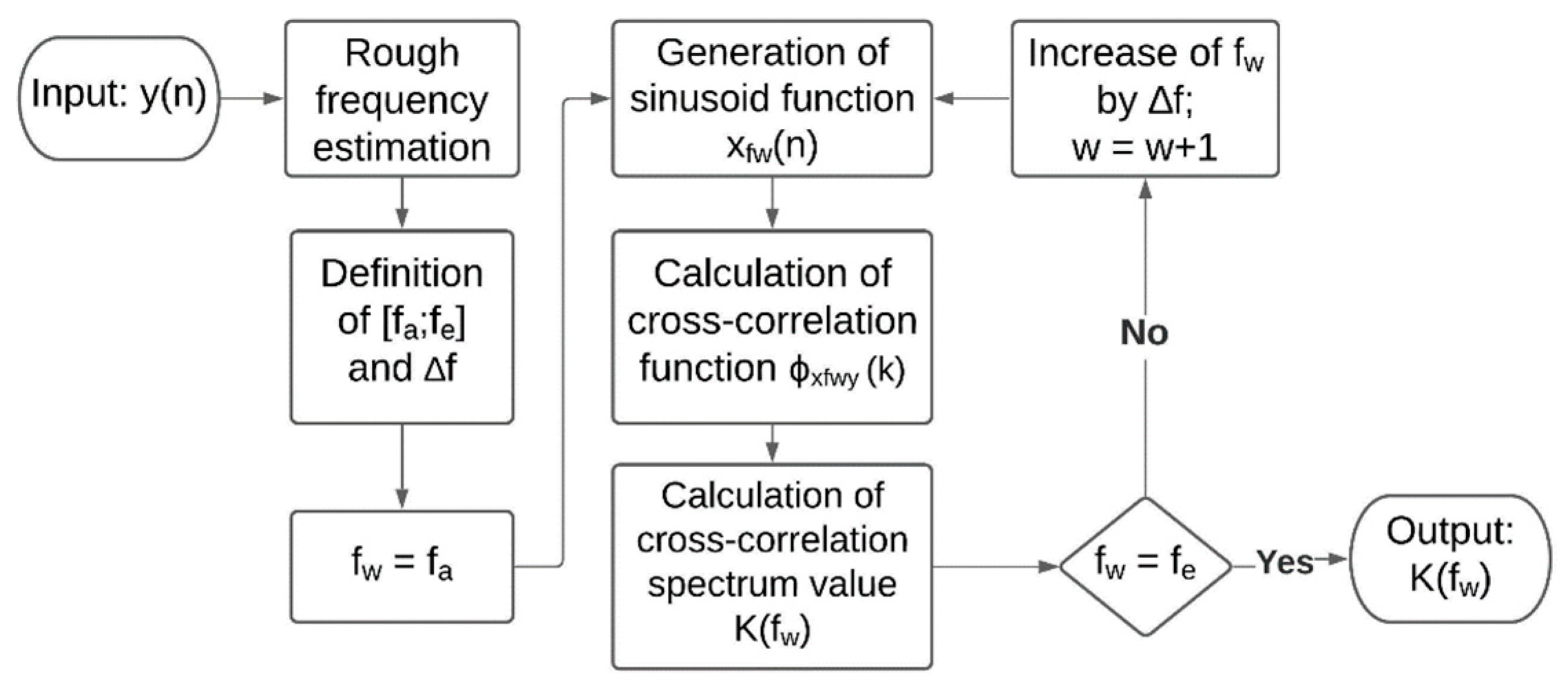
The CCS can be generated as followed (see Figure 1):

1.

The CCS’s frequency range $\left[f_a;f_e\right]$ and the frequency resolution $\Delta f$ are set by the user. $w$ is set to 0;

2.

$f_w$ is initialized to $f_a$ ($f_w=f_a$);

3.

The sine function $x_{f_W}\left(n\right)$ is generated according to Equation (17);

4.

The cross-correlation function ${\varphi }_{x_{f_w}y}\left(k\right)$ between the $x_{f_W}\left(n\right)$ and the measuring signal $y\left(n\right)$ is calculated;

5.

The cross-correlation spectrum’s value $K\left(f_w\right)$ for the current frequency $f_w$ is determined by identifying the amplitude of the cross-correlation function ${\varphi }_{x_{f_w}y}\left(k\right)$. In [13], it is accomplished by finding the function’s maximum value;

6.

The frequency $f_w$ is increased by $\Delta f$, i.e., $w=w+1$;

7.

The steps from 3–6 are repeated, until $K\left(f_w=f_e\right)$ has been determined.

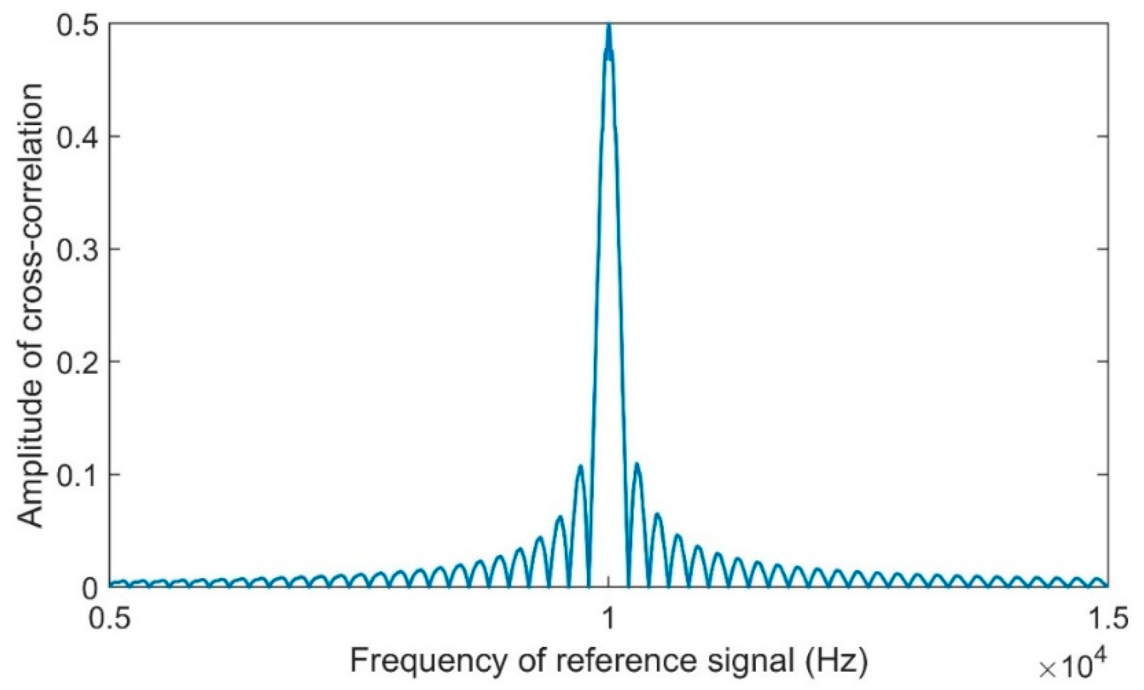
Figure 2 visualizes an exemplary CCS. Here, a simple sine function of the frequency 10 kHz is used as the measuring signal. The result resembles the absolute function of a sine cardinal, which has its global maximum at the measuring signals’ frequency. That makes the CCS a valid method to generate information about the frequencies of the measuring signal [9].

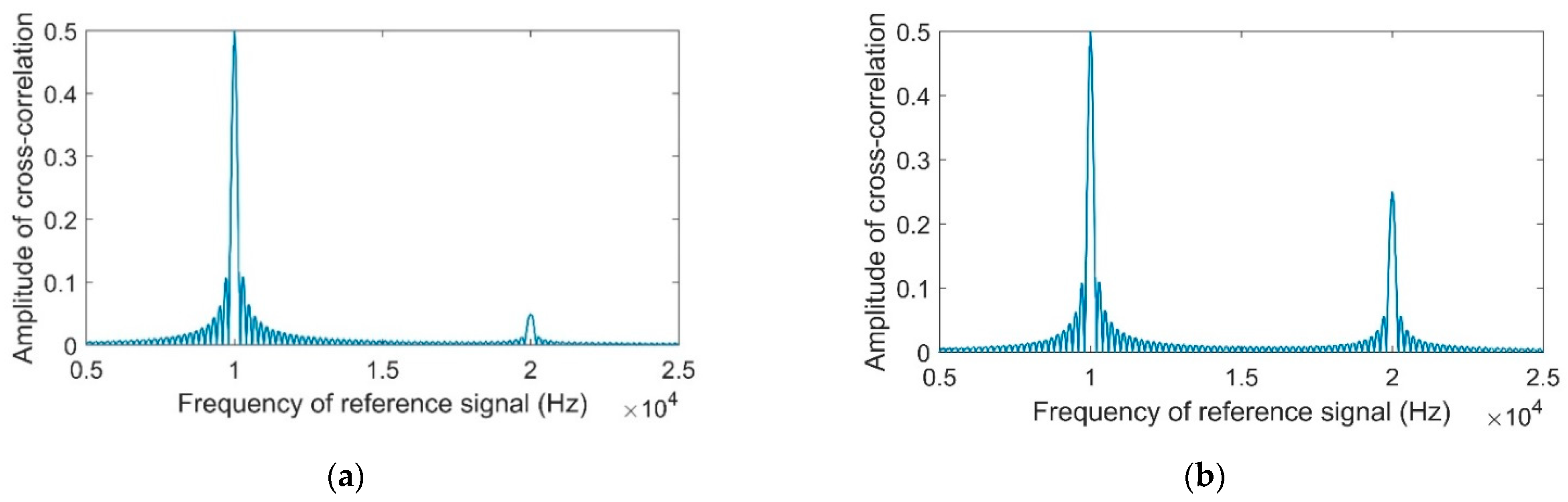
In Figure 3 the method’s ability to determine multiple signal frequencies is verified by adding a harmonic with a frequency of 20 kHz to the signal from Figure 2. In the resulting CCS, you can see two local maxima, which are positioned at the signal’s frequencies. The maxima’s value seems to depend on the corresponding harmonic’s amplitude. So, the method can not only recognize the different frequency components of the measuring signal, but their relative amplitude ratios as well [9].

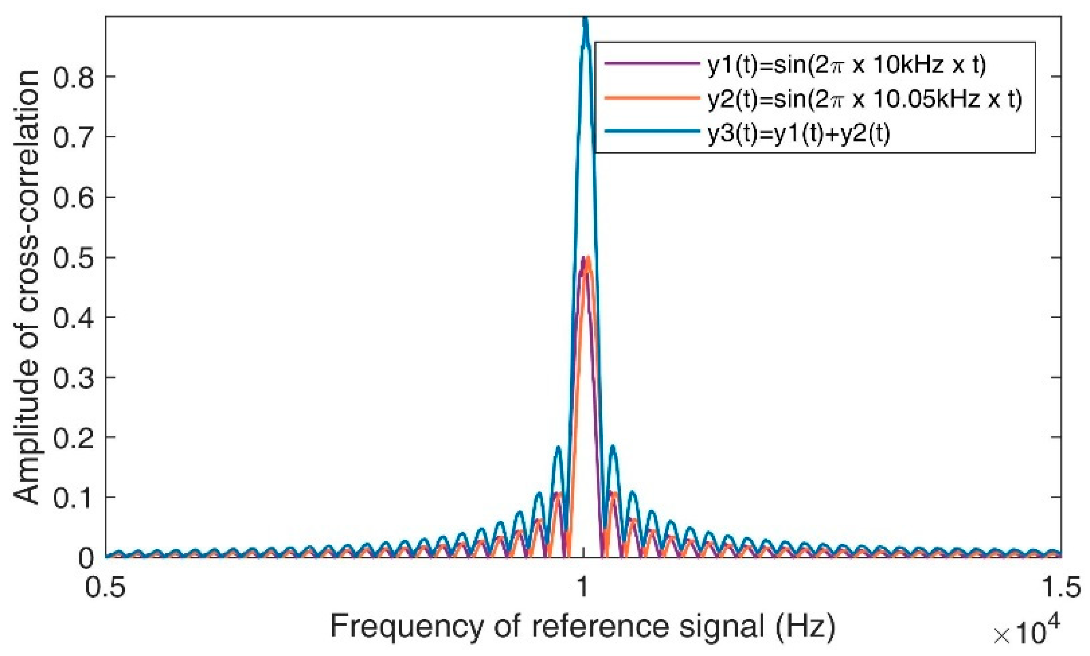
If the signal frequencies are close to each other, the resulting spectrum becomes the superposition of the functions representing the respective frequencies. This is shown in Figure 4, which visualizes the CCSs of two simple sine functions with different frequencies as well as the spectrum of the two sine functions’ sum [9].

In contrast to FFT and CWT, the frequency and time resolution of the CCS are not dependent from each other. Both can be set separately by the user. Thus, resolution problems can be reduced to a minimum. CCS makes frequency measurements with high time and frequency resolutions possible. Therefore, many limitations associated with FFT and CWT can be prevented with CCS [9].

However, the generation of a CCS in its current version is computationally intensive. In [9], each spectrum value $K\left(f_w\right)$ is determined by calculating at least one period of a cross-correlation function and finding the period’s absolute maximum value. This makes real-time application very difficult. Thus, a new version of the cross-correlation spectrum with reduced processing time is described in the following sections.

3. New Version of Cross-Correlation Spectrum

3.1. Theory

To reduce processing time, a new calculation method of $K(f_w)$ is required. For this purpose, Equation (11) has been analyzed. To gain $K(f_w)$, the largest absolute value of Equation (11) must be determined. This applies if the Equations (20) and (21) are fulfilled.

$$\cos \left(2\pi \ast f_y\ast \tau +\left({\phi }_x-{\phi }_y\right)\right)=\pm 1$$

(20)

$$2\pi \ast f_y\ast \tau +\left({\phi }_x-{\phi }_y\right)=z\ast \pi \hspace{1em}z\in {{\rm N}}_0.$$

(21)

The processing time is minimized, if only one value of the cross-correlation function is required to gain $K(f_w)$. To achieve that, one value of τ, which fulfills Equations (20) and (21), is needed. Under the following condition, $\tau =0$ would fulfill the requirements.

$${\phi }_x={\phi }_y.$$

(22)

This case represents the foundation of the processing method presented here. Since the phase ${\phi }_x$ is part of the reference signal, it can be determined by the user himself. If the user has precisely determined the phase of the measuring signal ${\phi }_y$, he can equate ${\phi }_x$ with ${\phi }_y$. In this case, only the cross-correlation value at $\tau =0$ needs to be calculated, to determine the amplitude of the cross-correlation function. That way, the calculation effort for the cross-correlation spectrum can be significantly reduced.

3.2. Simulations

In the following, simulations are carried out to verify the new method and compare it with the previous version of CCS. At first, symmetrical cross-correlation is used to generate the new version of CCS.

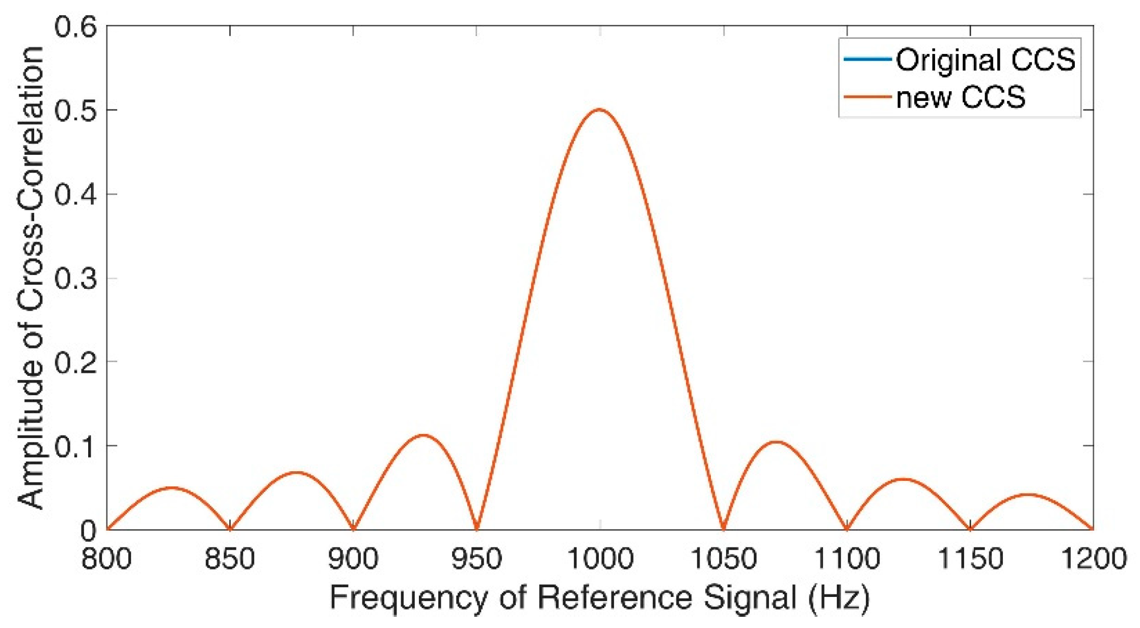
The first simulation generates the CCS with the new and the previous calculation method under the same conditions. The signal phase is known and is used in the new calculation method.

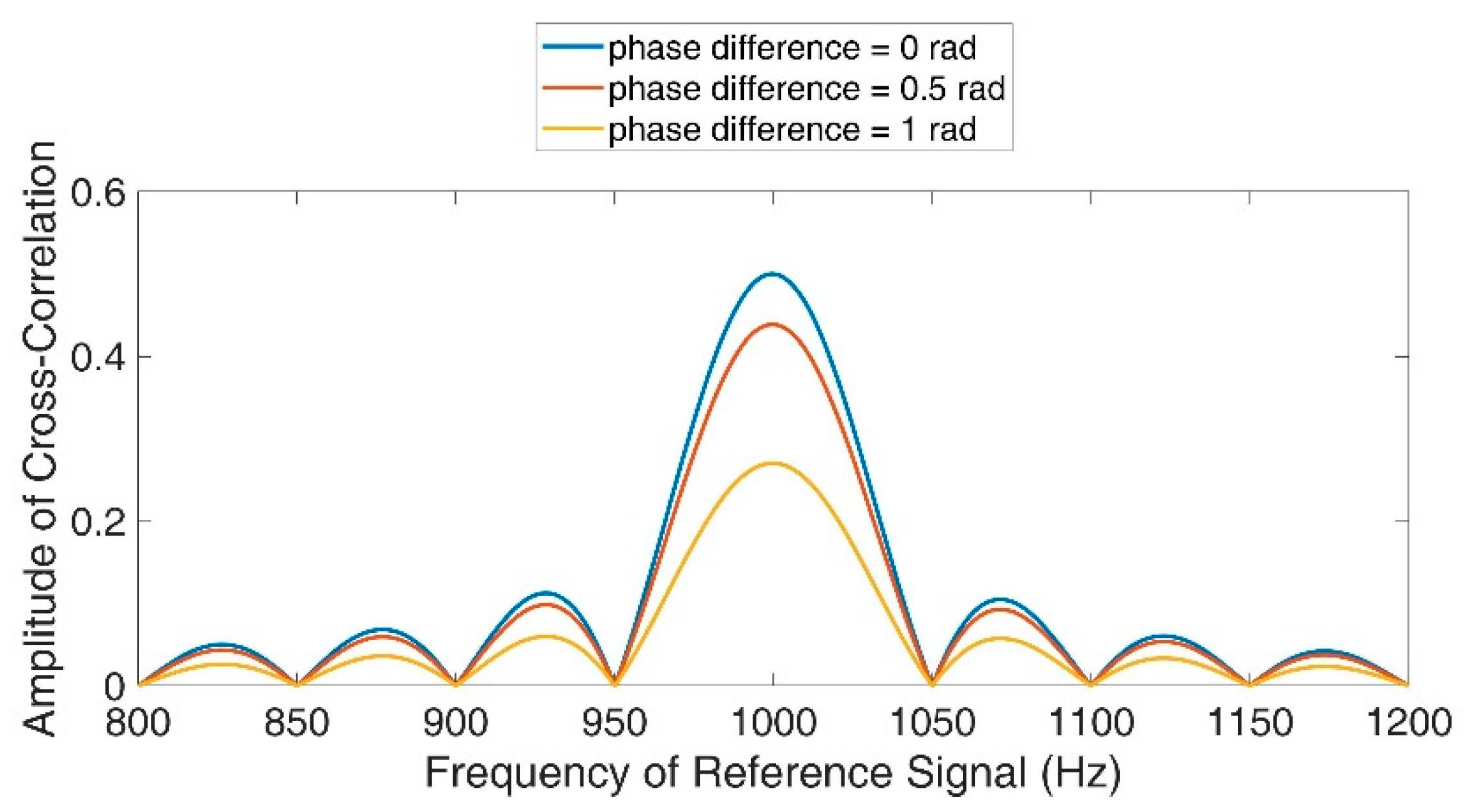
Figure 5 shows the resulting spectrums. If the phases of the reference and measuring signal match each other, there is no difference between the two versions, but in the new calculation method, information about the measuring signal phase is relevant and influences the amplitude of the cross-correlation function. For this reason, the next simulation investigates the extent to which phase differences between the reference and measuring signals affect the shape of the CCS. The result is visualized in Figure 6. The form of the CCS remains the same as the measuring signal’s phase increases, but its amplitude is reduced.

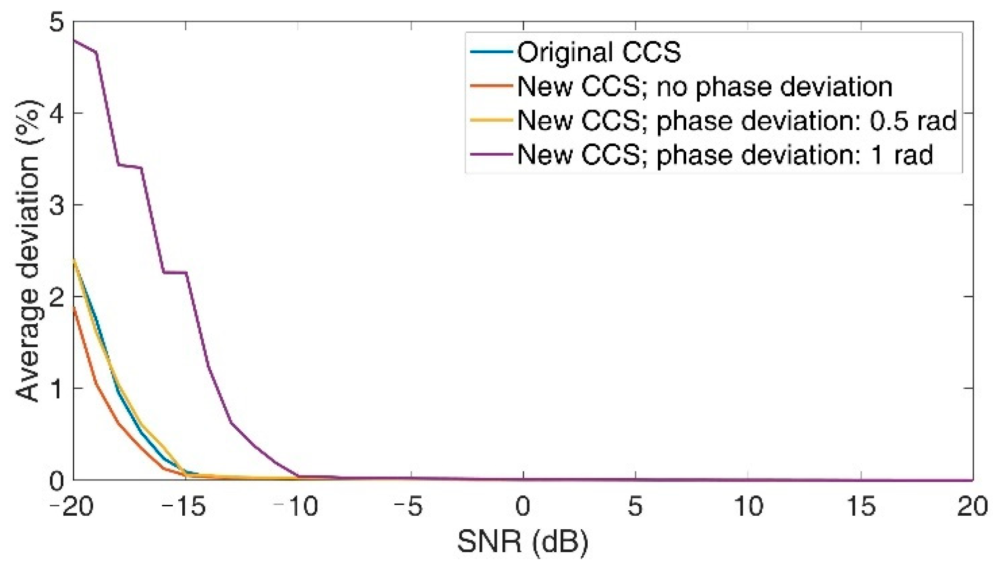
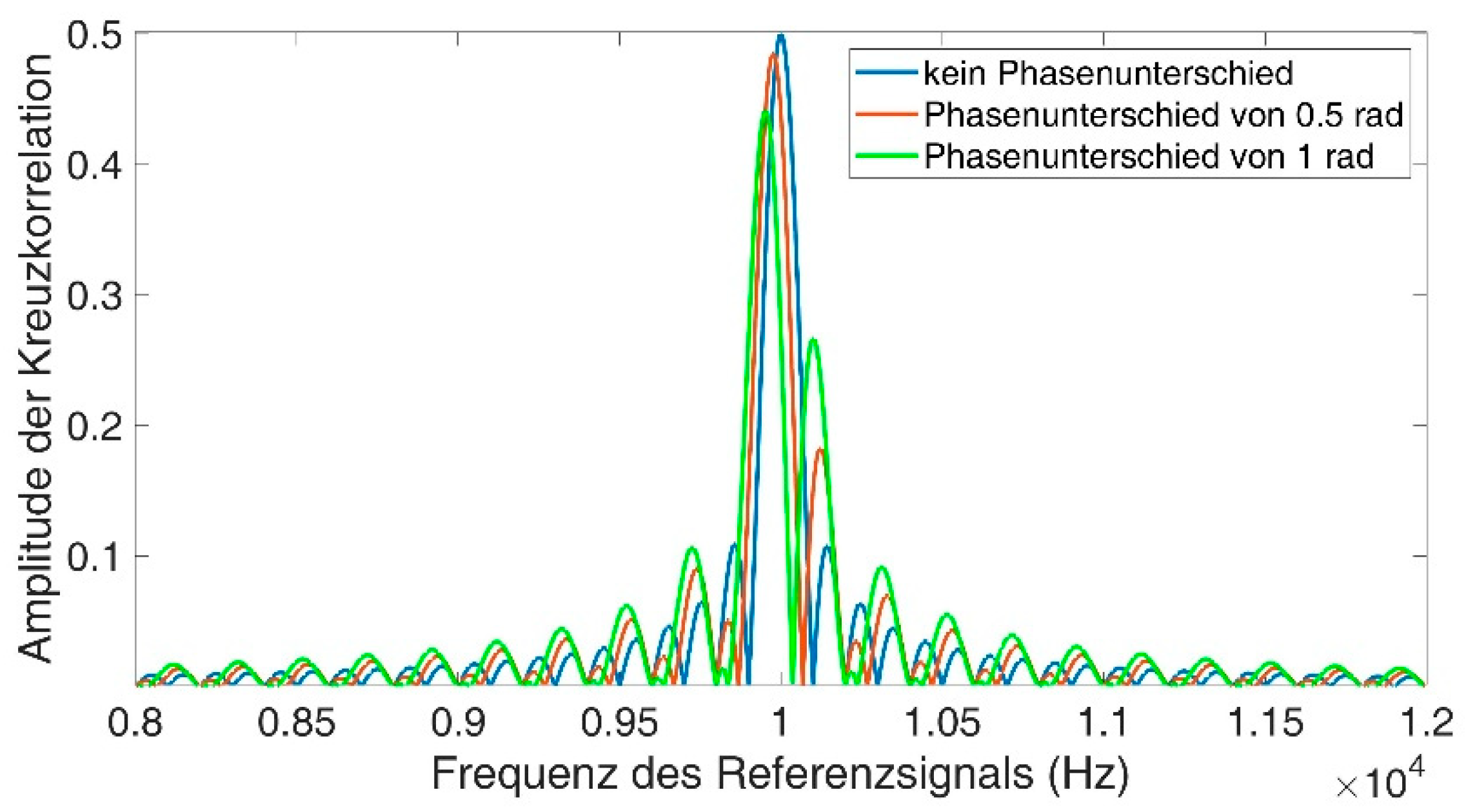
In the following simulation, the accuracy of the new CCS is analyzed on signals with different SNRs and subsequently compared with the previous method’s accuracy. Furthermore, the influence of phase information on the accuracy has been analyzed by setting the phase difference between reference and measuring signals to 0.5 and 1 rad. For each SNR, the frequency of 300 measuring signals was determined using both CCS versions. In each case, the signal length was 2000 data points. The results are visualized in Figure 7.

In the case of no phase deviation between reference and measuring signal, the new CCS shows the better results. If the noise suppression is insufficient, the previous CCS version proves to be more susceptible to interference than the new one. Beginning from a SNR of −4 dB, the new method’s accuracy is 0.01%. Above 9 dB, the accuracy is even below 0.001%. Thus, the new CCS using symmetrical cross-correlation is not only able to reduce the calculation time, but it can also improve the measuring accuracy, if correct phase information is available. However, with increasing the phase difference between reference and measuring signal, the accuracy deteriorates. With a deviation of 0.5 rad the new CCS’s accuracy is similar to the original CCS’s one. At 1 rad, the accuracies have become worse. However, even in this case, the frequency measurements are precise for SNR above −10 dB.

In general, the relationship between the phase difference and the new CCS’s accuracy is described in

Table 1. Relationship between phase difference and the new CCS’s accuracy.

Phase Difference	Behavior of Accuracy
$\left[0;0.5\pi \right]$	Increasing phase difference leads to accuracy deterioration
$\left[0.5\pi ;\pi \right]$	Increasing phase difference leads to accuracy improvement
$\left[\pi ;1.5\pi \right]$	Increasing phase difference leads to accuracy deterioration
$\left[1.5\pi ;2\pi \right]$	Increasing phase difference leads to accuracy improvement

.

This behavior can be explained mathematically. If Equation (1) is used in Equation (18) and the condition $\tau =0$ taken into account, the following equation arises:

$$K\left(f_w\right)=|{\varphi }_{x_{f_w}y,symm}\left(0\right)|=|\cos \left({\phi }_y-{\phi }_x\right)\frac{A\ast B\ast (\sin \left(2\pi \ast T\ast \left(f_x-f_y\right)\right)}{T\ast 4\pi \ast \left(f_x-f_y\right)}|.$$

(23)

Here, the CCS is an absolute sine-function, whose amplitude reduces with increasing difference between $f_x$ and $f_y$. The relationship between the phase difference $({\phi }_y-{\phi }_x)$ and the CCS’s amplitude is a cosinus-function and leads to the CCS’s accuracy behavior shown in Table 1.

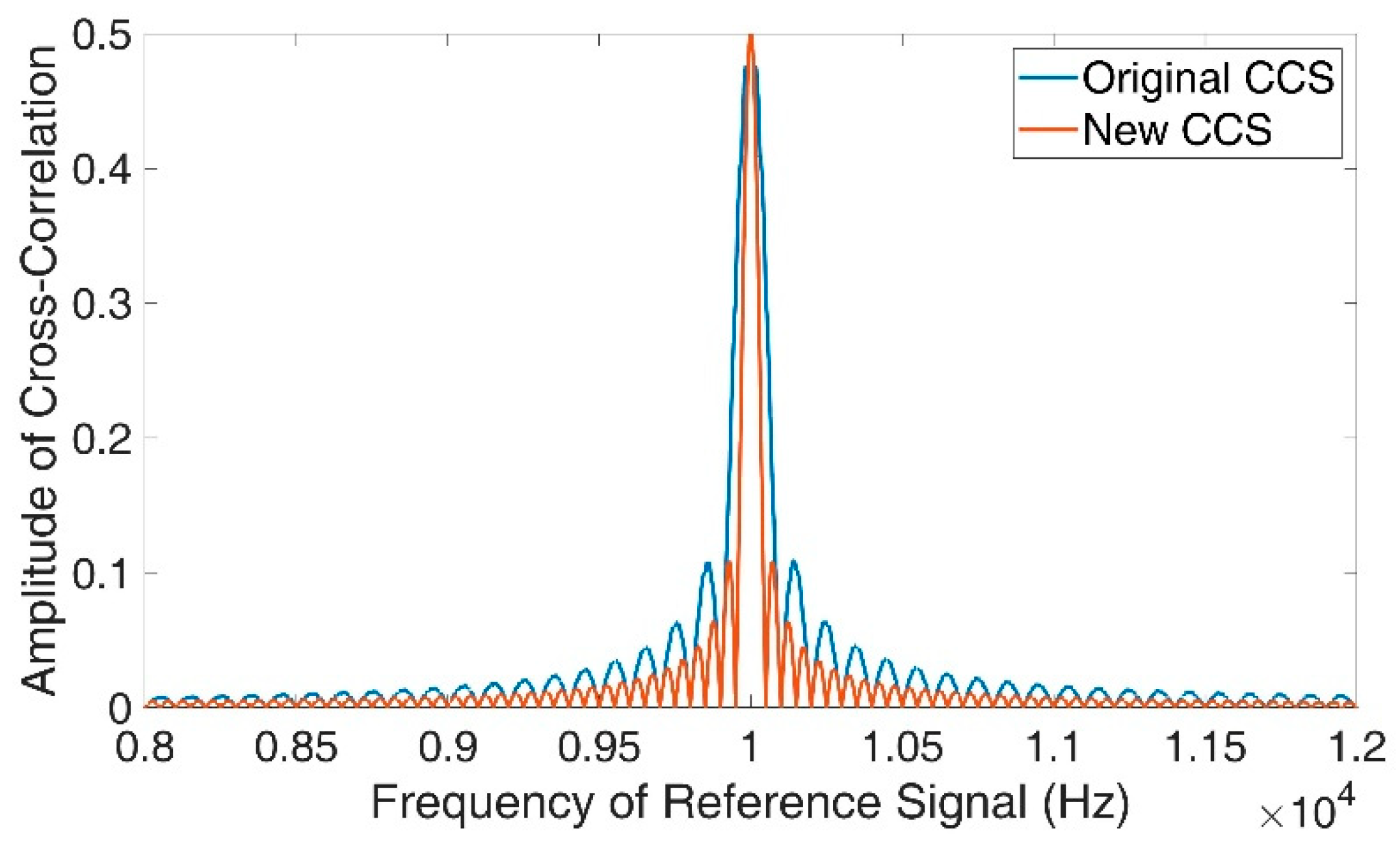
The following simulations analyze the new method‘s performance using the asymmetrical cross-correlation function. At first, the simulation of Figure 5 is repeated using asymmetrical cross-correlation and its results are visualized in Figure 8.

Both spectra are sinc-functions. However, the CCS of the new calculation method is much narrower, if asymmetrical cross-correlation is used. The behavior of the simplified cross-correlation spectrum with asymmetrical cross-correlation can be justified mathematically. If Equation (3) is used in Equation (18) and the conditions ${\phi }_x={\phi }_y$ and $\tau =0$ are taken into account, the following equation results:

$$K\left(f_w\right)=|{\varphi }_{x_{f_w}y,unsymm}\left(0\right)|=|\frac{A\ast B\ast (\sin \left(2\pi \ast T\ast \left(f_x-f_y\right)\right)}{T\ast 4\pi \ast \left(f_x-f_y\right)}|.$$

(24)

Compared to Equation (8), which describes the amplitude of the regular cross-correlation spectrum, the angular velocity $\omega =2\pi \ast T$ of the sine component has doubled in Equation (24). This explains, why only half as many data points are required for the same compression. This can be considered a positive result, as the CCS becomes more precise this way.

The next simulation examines, how the usage of the asymmetrical cross-correlation affects the new CCS, when there are phase differences between the measuring and reference signals. Figure 9 compares the CCS with and without phase differences.

The new CCS with asymmetrical cross-correlation is significantly deformed by the phase differences. This behavior can be explained mathematically as well. If Equation (3) is used in Equation (18) and only the condition $\tau =0$ is taken into account, the following equation is derived:

$$K\left(f_w\right)=|{\varphi }_{x_{f_w}y,unsymm}\left(0\right)|=|\frac{A\ast B\ast (\sin \left(2\pi \ast T\ast \left(f_x-f_y\right)+\left({\phi }_x-{\phi }_y\right)\right)-\sin \left({\phi }_x-{\phi }_y\right))}{T\ast 4\pi \ast \left(f_x-f_y\right)}|.$$

(25)

The phase difference between the reference and measuring signal $\left({\phi }_x-{\phi }_y\right)$ has a clear influence on the amplitude function $K\left(f_w\right)$. This leads to the deformations and makes frequency measurement more difficult.

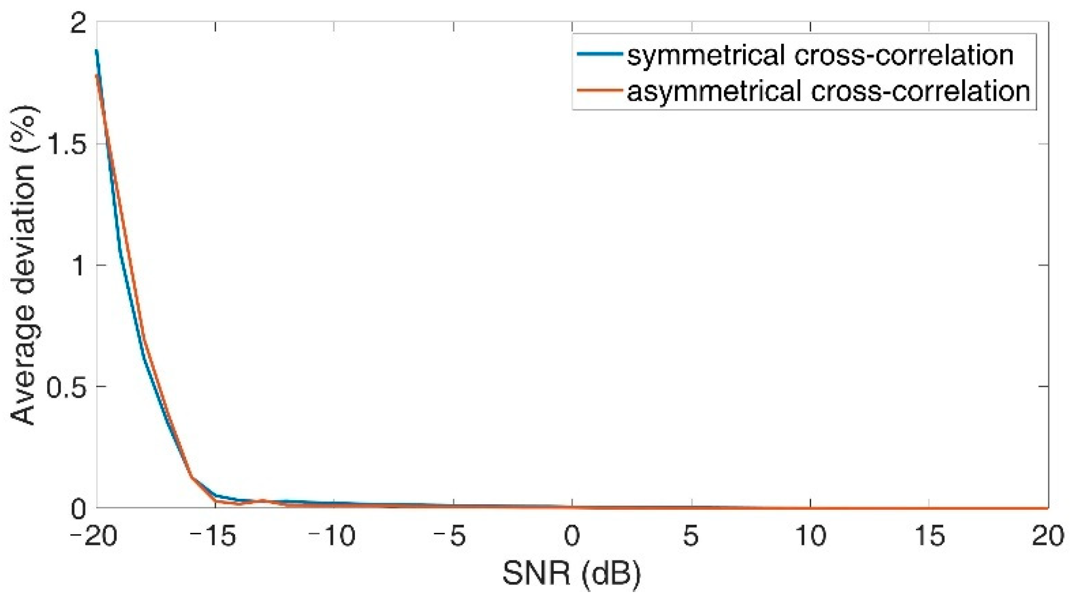
The next simulation examines the frequency measuring accuracy of the new CCS, if either symmetric or asymmetric cross-correlation is used. For each SNR, the frequency of 300 measuring signals was determined using both methods. The signal length is 2000 data points and correct phase information is used. The results are visualized in Figure 10.

If the phase information is correct, the used cross-correlation version does not appear to have any significant impact on the frequency measurement accuracy. Even though a finer spectrum is created with asymmetrical cross-correlation, the noise reduction remains the same.

4. Phase Measurement Using Cross Correlation

In the following simulations, the use of asymmetrical and symmetrical cross-correlation in phase measurement is tested. The idea is to generate the cross-correlation between the measuring signal and the reference signal described by Equation (26). Afterwards, the measuring signal’s phase ${\phi }_y$ is measured by determining the cross-correlation function’s phase ${\phi }_{{\varphi }_{xy}}$ using the discrete Fourier series (=DFR) and Equation (27). That way, a reduction of noise power and subsequently more precise phase measurement should be achieved.

$$x\left(t\right)=\sin \left(2\pi \ast f_x\ast t\right)$$

(26)

$${\phi }_y={\phi }_{{\varphi }_{xy}}-\frac{\pi }{2}.$$

(27)

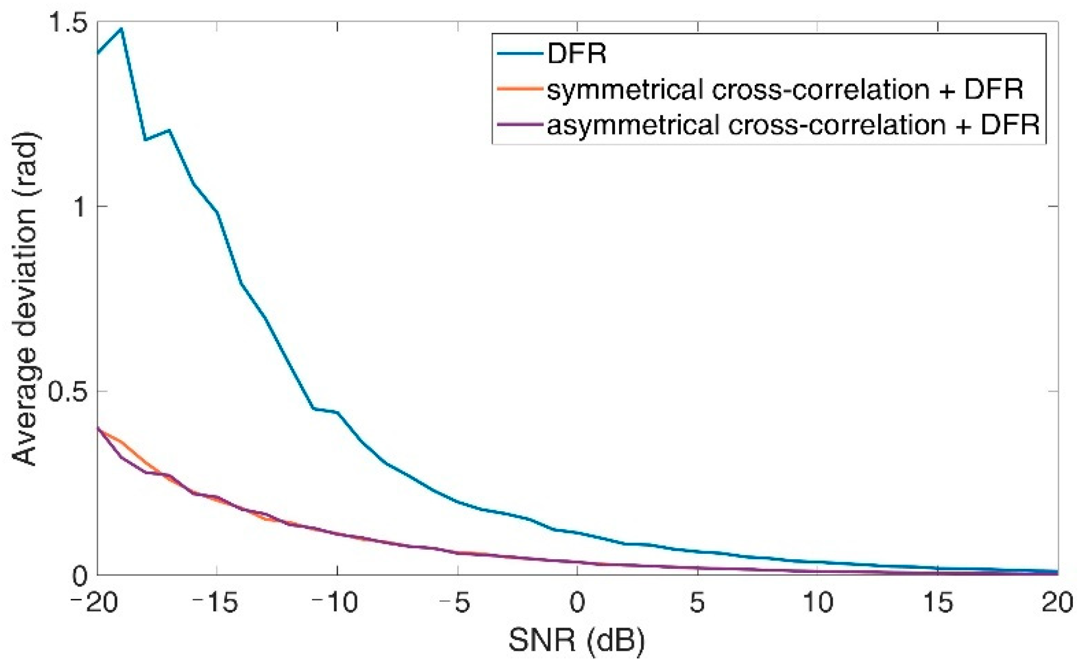
Next, the measurement method’s performance is evaluated at different SNRs and compared with the accuracies achieved by simply using DFR. A noisy sinusoidal signal with a frequency of 1 kHz and a phase of 1.23 rad, which was sampled at a frequency of 100 kHz, is considered. The cross correlation function is generated with a reference signal of the same frequency as the measuring signal. The result is visualized in Figure 11.

Significant improvements result from the use of cross-correlation. The version of the cross-correlation function does not influence the accuracy in these circumstances. Even with an SNR of 0 dB, the average error is below 0.04 rad. At lower SNR, the error increases, but even with an SNR of −20 dB, the average error is below 0.5 rad and thus significantly lower than without cross-correlation.

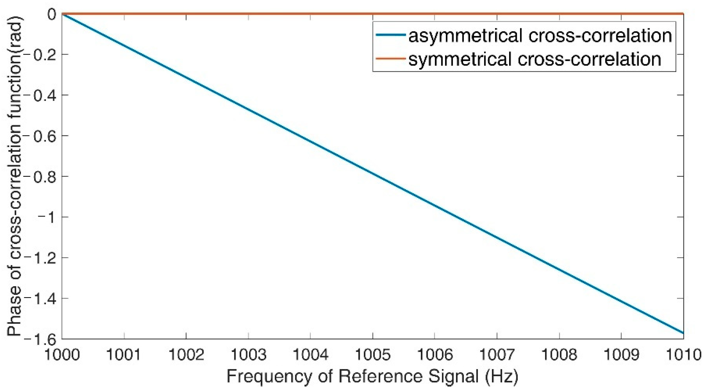
In reality, you cannot assume that the reference and measuring signal have the same frequency. Therefore, it is important to analyze how the method performs, if a frequency difference between the reference and measuring signal exists. At first, the method has been tested with noise-free signals. The reference signal’s frequency is varied in 0.05 Hz steps between 1000 and 1010 Hz, while the frequency and phase of the measuring signal is 1000 Hz and 0 rad. 500 data points have been used for the cross-correlation function. Figure 12 shows the measured phases using both versions of the cross-correlation function.

If asymmetrical cross-correlation is used, the frequency differences cause a phase shift in the cross-correlation function, which is proportional to the frequency difference. The symmetrical cross-correlation does not have this issue. Thus, moving forward, only symmetrical cross-correlation is going to be considered for phase measurement.

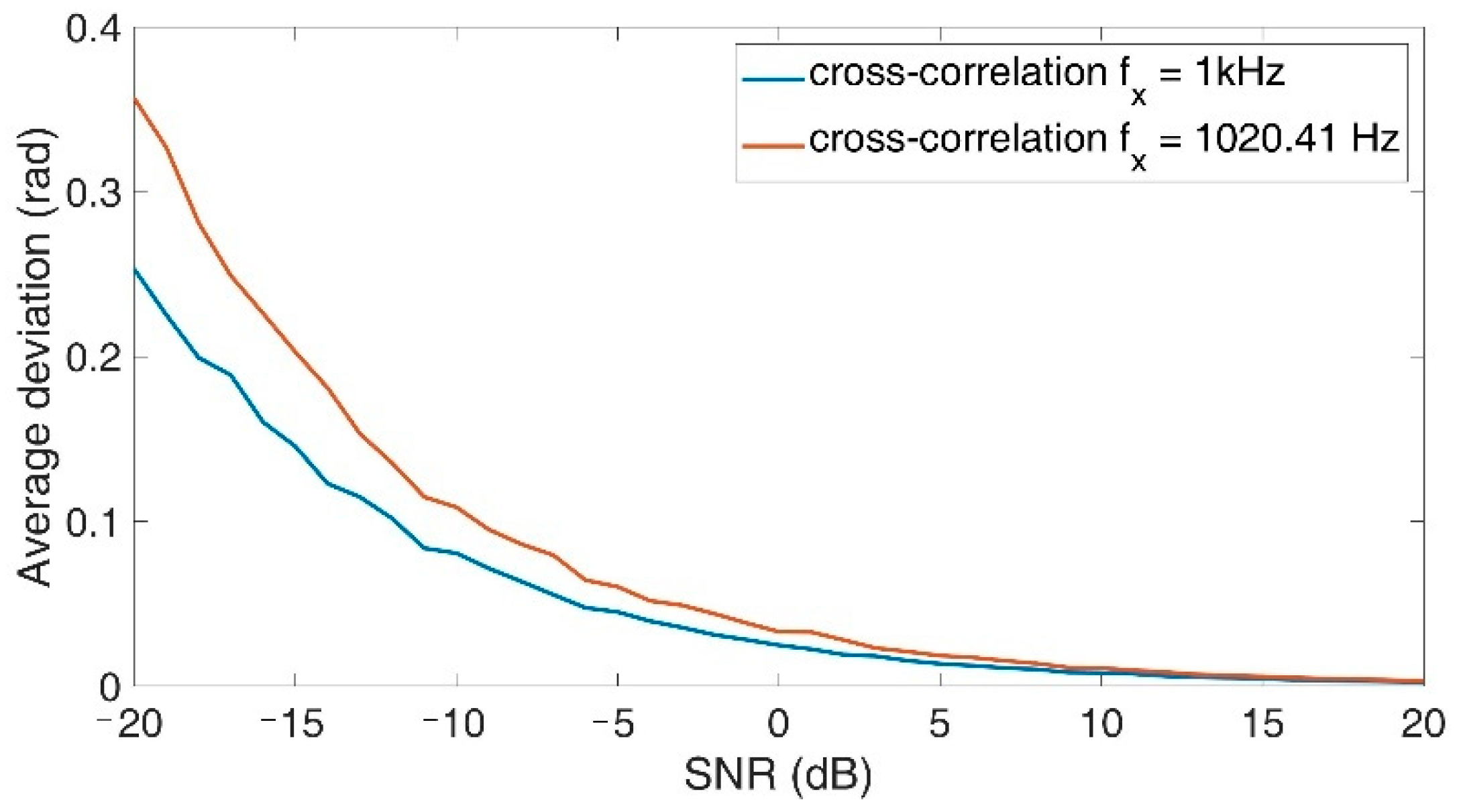
The last simulation examines which influence frequency differences between reference and measuring signal have on the method’s accuracy. The reference signal’s frequency is set to 1020.41 Hz and the accuracy compared to the one without frequency differences. The results are shown in Figure 13.

As the frequency difference increases, the average phase deviation does so as well. This is mainly due to the fact that the amplitude of the cross-correlation function and thus also the SNR of the cross-correlation function decreases as the frequency difference increases. So overall, phase measurement using cross-correlation is possible in the case of frequency differences. However, the more accurate the frequency information is, the better the results.

5. Frequency and Phase Measurement Method

Section 3 has shown that the new CCS can not only reduce processing time but can also achieve frequency measurements that are as accurate as with the original CCS. However, phase differences between the reference and measuring signals lead to undesired changes in the spectrum. Before using the new CCS in frequency measurements, correct phase information has to be available. With the symmetrical cross-correlation function, accurate phase measurements of noisy signals are possible but, here, frequency differences between the reference and measuring signals have a negative effect on the phase measuring accuracy. Thus, there is a correlation between the new CCS and the phase measurement method using cross-correlation. The output of one method is the input of the other one and vice versa.

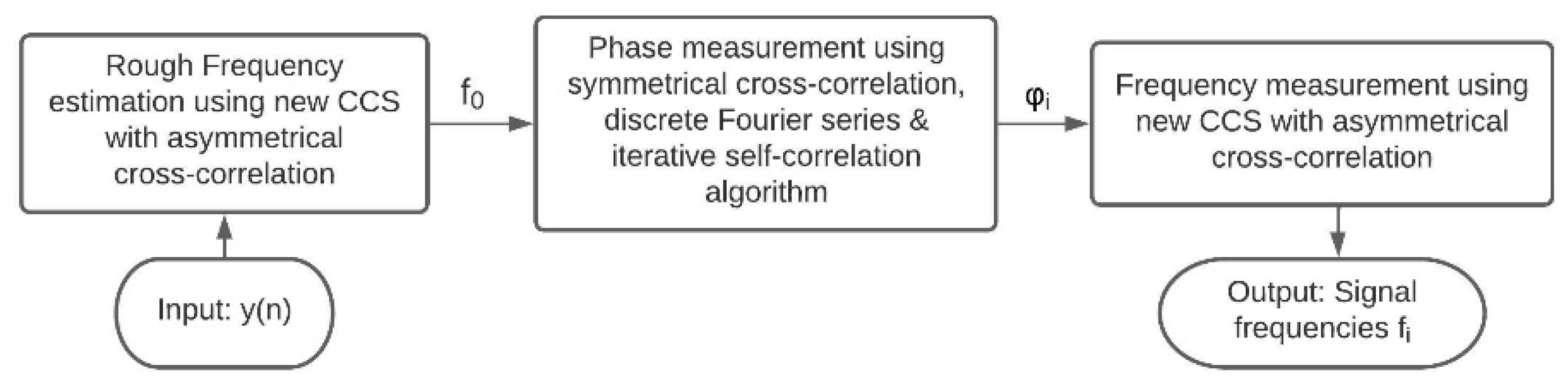
Based on these findings, a new method has been developed, which is visualized in Figure 14. After rough frequency estimation with the new CCS, the signal phase is measured using a symmetrical cross-correlation function and a discrete Fourier series. Afterwards, the new CCS method is repeated with the phase information, to measure the frequency accurately. For the new CCS, asymmetrical cross-correlation is used, as it provides a finer and thus more precise spectrum (see Figure 8), where the risk that the sinc-functions of frequencies mix with each other is significantly reduced. The iterative self-correction algorithm of [14] is used in the phase measurement to reduce errors due to the asynchrony between the signal and sampling frequency.

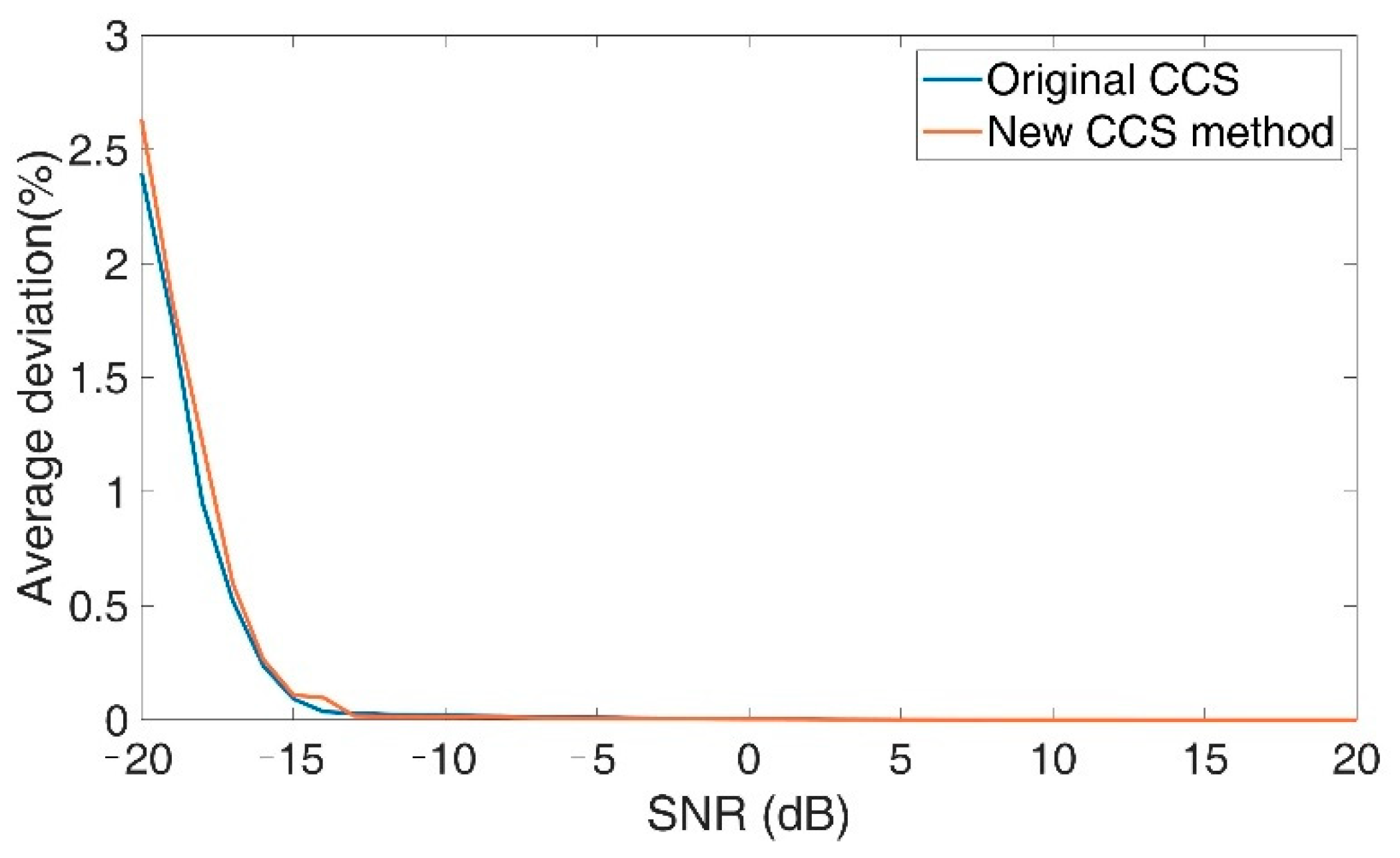
Figure 15 shows the frequency measuring accuracy of the new CCS method compared to the original CCS’s one. In the simulation, the frequency of 300 measuring signals for each SNR was determined with the methods. Signal sections with a length of 2000 data points have been used in both methods.

Compared to the original CCS, the new CCS method’s accuracy is only slightly worse. In SNRs higher than −14 dB the new method shows an accuracy of 0.1% in the frequency measurement. Beginning from −7 dB, the accuracy is at 0.01%. Considering that the calculation time can be significantly reduced with the new method, the results are convincing.

The following simulation will examine the processing times of the original CCS and the new CCS method. Both methods are carried out on a signal with a frequency of 1 kHz and the calculation times are recorded. The sampling frequency is 100 kHz. For the CCS, the resolution and the frequency range under consideration have been set at 1 Hz and 900 to 1100 Hz. 2000 data points are used for the cross-correlation spectra, while 500 data points are used for the cross-correlation function of the phase measurement. In

Table 2. Average processing time of original CCS and the new method.

Original CCS	New CCS Method
286.93 ms	30.82 ms

the average processing times of both methods with the described settings are visualized. With the new CCS method, the processing time can be reduced by 89.26%, which proves to be a significant improvement.

6. Application Example

6.1. Self-Mixing Interferometry

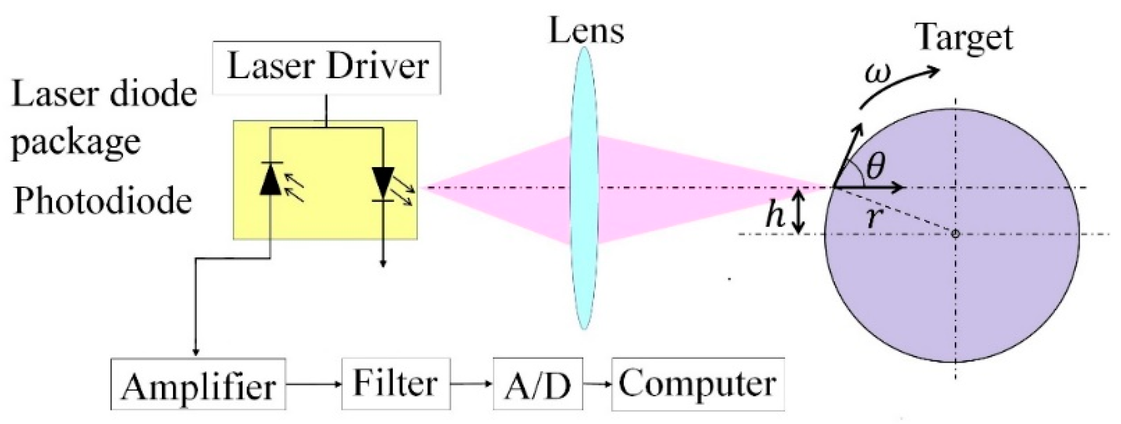
As in [9], the new CCS method’s accuracy to measure frequencies will be validated on SMI signals. SMI is a measurement technology, in which a laser beam is reflected from a target object, back into the laser cavity (see Figure 16). This results in interferences between the light generated inside the laser and the reflected one, which change the laser’s amplitude and frequency. When a built-in photodiode senses the laser’s output power, one can obtain a signal (=SMI-signal), which can be used for measurements of physical properties such as displacement, speed or vibration [15]. If a turntable is used as the target object, a linear relationship between the SMI-signal’s frequency (=Doppler frequency) $f_D$ and the turntable’s rotational speed $\omega$ exists (see Equation (28)) [7,9]:

$$f_D\left(\omega \right)=\frac{2\ast \omega \ast r\ast \cos \left(\theta \right)}{\lambda }.$$

(28)

$\lambda$ represents the laser diode’s wavelength, while $r$ and $\theta$ symbolize the target object’s radius and the incident angle between the laser and the target object’s moving direction.

With SMI-signals, the direct measurement of the target’s rotational speed is possible. Because of the method’s inherently high resolutions [16], which are not influenced by the target’s speed, there are no resolution issues in low-speed ranges. Therefore, self-mixing interferometry has become a promising solution for rotational speed measurements.

Figure 16. Schematic structure of SMI rotational speed measurement (Adapted/Reprinted with permission from [7,17] © The Optical Society).

Figure 16. Schematic structure of SMI rotational speed measurement (Adapted/Reprinted with permission from [7,17] © The Optical Society).

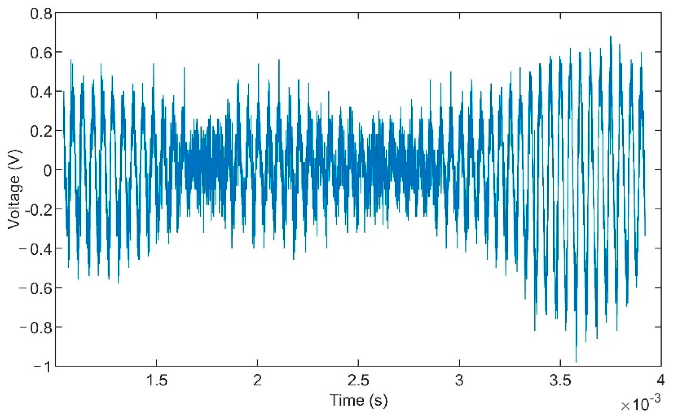
Many issues are linked to the usage of self-mixing-interferometry. A major one is spectral broadening. It results from different aspects such as the vibration, speckle effect and profile add uncertainty, change of surface or velocity distribution over the light spot region [18] and results in frequency and amplitude modulations of the SMI signal [19]. Ref. [20] has conducted a comprehensive analysis of factors influencing the spectrum of the SMI signal and identified a vast list of major and minor elements. Besides spectral broadening, the SMI-signal is often corrupted by dynamic offsets due to environmental influences, system instabilities or by additive noises [16], which are caused by environmental aspects such as electromagnetic interferences etc. [9].

Figure 17 shows a typical SMI signal. It is a sinusoidal signal that is disturbed by additive noise as well as frequency and amplitude modulation. All these factors complicate the precise measurement of rotational speed using self-mixing interferometry. Thus, robust signal processing methods are required.

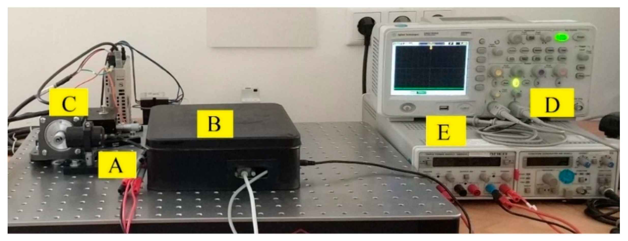
To obtain SMI-signals for the experiments, the same test system as in [9] is used (see Figure 18). A laser driver turns the power supply’s output into a constant current, which runs a sensor head consisting of two lenses and a commercial 785 nm laser diode with an integrated photo diode. The sensor head targets a turntable mounted on the shaft of a Yaskawa SGMJV-02A3E6S servo motor. The motor is controlled by a computer with the servo drive Yaskawa SGDV-1R6A01B002000 and rotates the turntable with a constant rotational speed. To provide a good velocity reference, the speed is measured by a 21-bit optical encoder [15]. The integrated photo diode detects the optical feedback, generated by self-mixing interferometry, and sends its output to a preprocessing circuit. Finally, the circuit extracts and amplifies the SMI-signal and sends it to an oscilloscope for further analysis. The test system uses an 8-bit DSO1024A oscilloscope of Agilent with a bandwidth of 200 MHz [9].

The experiments are designed to validate the method’s ability to detect signal frequencies and analyze its measurement accuracy. Because of spectral broadening, the original frequency of the SMI signal is estimated with the same estimation method as in [9]. Furthermore, the averaging window from [9] is used to compensate errors due to frequency modulation in the SMI signal.

With the new CCS method, one must take into account that only the phase of the signal part, whose frequency has the highest power in the viewed frequency range, is determined. Accordingly, only the sine cardinalis of the correlating signal part is visualized correctly in the CCS. The sinus cardinalis of the other signal frequencies can still show erroneous amplitudes. To determine the phases of all signal parts and to optimize the CCS accordingly, one should divide the viewed frequency range into several areas. Ideally, each area contains the frequency of one signal part. Then, the algorithm is carried out on each area. This way, the amplitudes of the respective signal frequencies are correctly visualized in the CCS.

6.2. Experiments on SMI-Signals

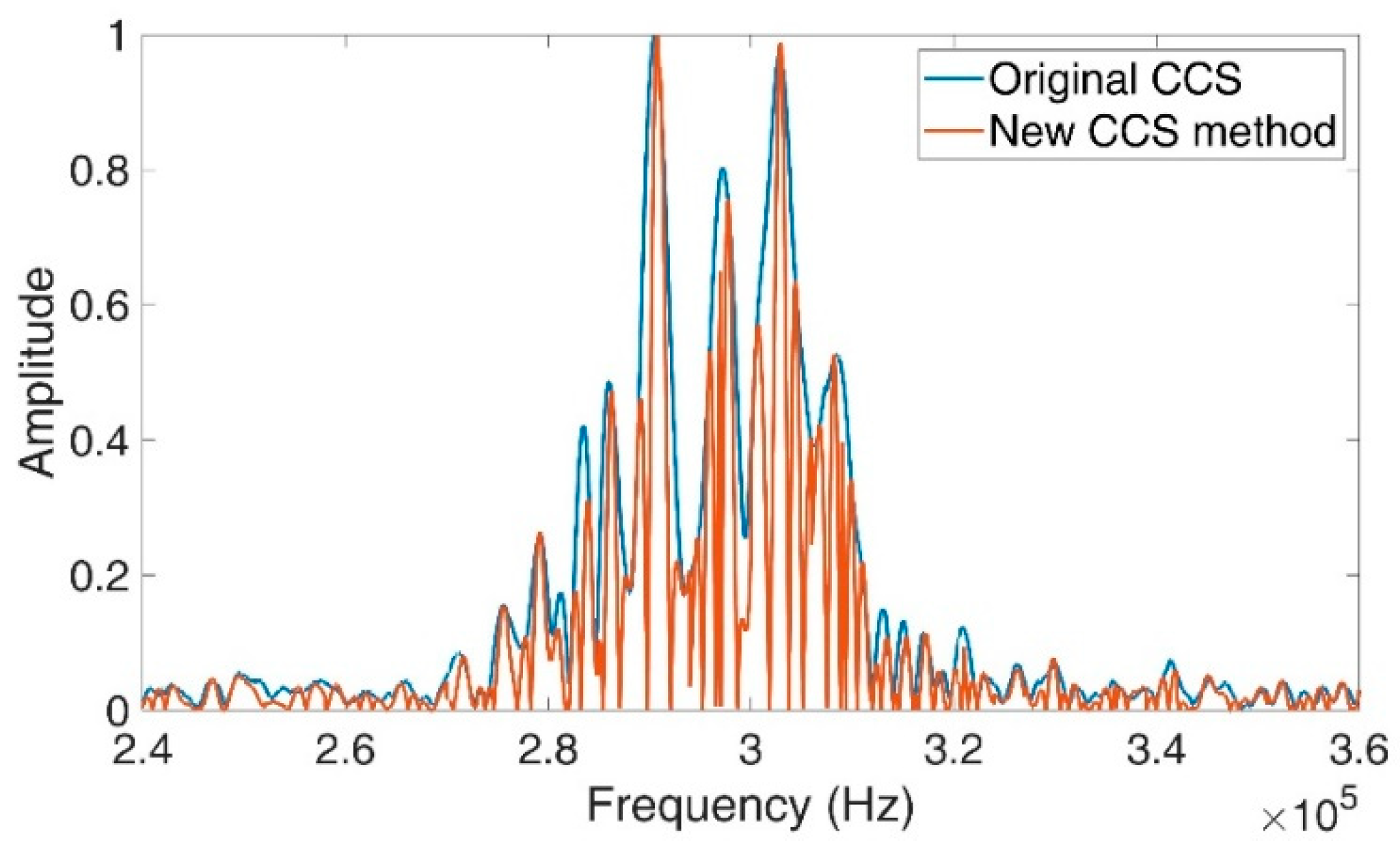
The first experiment aims to analyze how well the new method can provide information about a signal’s frequencies compared to the previous version of the CCS. Thus, the first experiment from [9] has been repeated with the new method. Figure 19 visualizes the CCS of the new method and the old CCS of an SMI signal with a length of 10,240 data points. The sampling frequency is 12.5 MHz.

Overall, the new CCS stays within the original one. Compared to the original CCS, the new one proves to be finer. Frequencies, which are close to each other, can be better distinguished from one another, since there is less risk that the sinc-functions of the respective frequencies mix with each other. Thus, the CCS has become more precise.

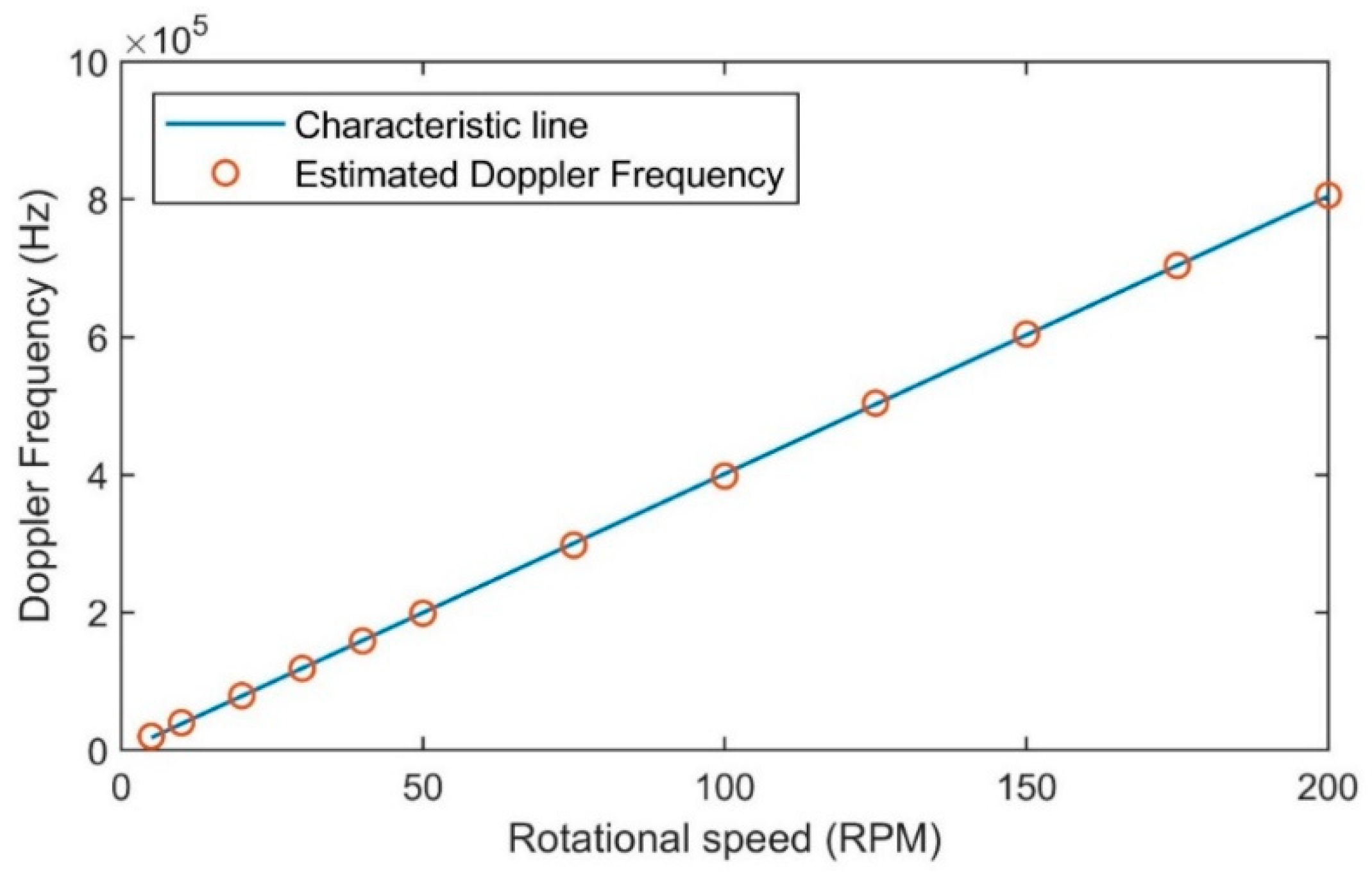
With the experiment setup from Figure 18, the new method’s ability to measure rotational speed is tested. According to Equation (26), one needs the incident angle to calculate the rotational speed from the Doppler frequency. However, if the laser’s direction, position and thus the laser incident angle is fixed, the characteristic line between rotational speed and Doppler frequency can be obtained by calibrating the measuring system. If the characteristic line is linear and its slope known, the rotational speed can be derived easily from the Doppler frequency. Therefore, the experiment aims at finding the linearity and accuracy of the proposed method in frequency measurement. The first 3000 data points of each dataset have been used for the CCS. In addition to that, the average window’s size has been set to 20. For each speed, the same frequency ranges as in [9] are used.

In the first step, the linearity between the results and the turntable’s rotational speed has been validated. For this purpose, a characteristic line has been created by using linear regression from the average values of 50 datasets for each rotational speed. Figure 20 visualizes the results, while

Table 3. Linearity of method in [17], original CCS and new CCS method.

Rotational Speed in RPM	Linearity of Method in [19]	Linearity with Original CCS	Linearity with New CCS Method
5	−0.21	−0.24%	+0.23%
10	−0.18	−0.20%	+0.20%
20	−0.10	−0.06%	+0.08%
30	+0.01	0.03%	−0.00%
40	+0.10	0.09%	−0.10%
50	+0.14	0.11%	−0.10%
75	+0.31	0.35%	−0.27%
100	+0.21	0.40%	+0.32%
125	−0.26	−0.21%	+0.14%
150	−0.12	−0.16%	+0.10%
175	+0.18	0.03%	+0.02%
200	−0.21	−0.12%	+0.18%

compares the linearity of the new method, the old CCS, and the method of [17], where a signal selection algorithm, autocorrelation and an averaging window are used for the measurement of the Doppler frequency.

Table 4. NRMSE of results using the method of [17], original CCS and new CCS method.

Rotational Speed (RPM)	NRMSE of Method in [19]	NRMSE with Original CCS (%)	NRMSE with New CCS (%)
5	0.16	0.16	0.18
10	0.06	0.06	0.07
20	0.05	0.08	0.09
30	0.08	0.14	0.13
40	0.15	0.18	0.21
50	0.13	0.13	0.12
75	0.07	0.04	0.05
100	0.06	0.06	0.07
125	0.06	0.06	0.09
150	0.07	0.08	0.08
175	0.05	0.06	0.07
200	0.06	0.03	0.03

shows the accuracy of the method in [17], the original CCS and the new method as the normalized root mean square error (=NRMSE) of its results. In both cases, the average Doppler frequencies of the respective velocities have been used as the reference of the NRMSE.

Table 4 shows that the new method can measure the Doppler frequencies accurately, as the NRMSE stays below 0.22%. Compared to the original CCS, the accuracy has deteriorated up to 0.04%. However, considering that the new method can reduce the calculation time by up to 89%, it can be considered significant progress. In comparison to the results in [17], the new method’s accuracy is worse as well. That is because the method in [17] has been specifically designed for SMI signals, while the CCS is supposed to be used for signal frequency measurements in general. Thus, the new method’s accuracy is still convincing. So altogether, the results of the new methodology prove to be promising and a significant advance in frequency measurement.

7. Discussions

In this paper, a new way to create the cross-correlation spectrum (CCS) for frequency measurements of signals with low SNR is presented. It aims to reduce processing time to enable real-time application.

In its original version, each spectrum value is determined by calculating at least one period of a cross-correlation function and finding the function’s absolute maximum value.

In the new CCS, the processing time is minimized by calculating only one value of the cross-correlation function. If the measuring signal’s phase is known, the reference signal’s phase can be given the same value. That way the cross-correlation function’s value at $\tau =0$ represents the CCS’s value. If asymmetrical cross-correlation is used for the new CCS, the resulting sinc-function becomes narrower and thus the spectrum more precise. Therefore, the method not only reduces processing time, but also provides better accuracies if the measuring signal’s phase is known. However, the new CCS with asymmetrical cross-correlation gets deformed by phase differences between the reference and measuring signals. This deteriorates the frequency measurement significantly.

To measure the phase of noisy signals, the discrete Fourier series of a symmetrical cross-correlation function between a reference signal and the measuring signal can be used. The cross-correlation function reduces the noise power and subsequently leads to more accurate results.

Based on the findings, a new CCS method has been developed. It consists of a rough frequency estimation using the new CCS with asymmetrical cross-correlation, a phase measurement using symmetrical cross-correlation and a final frequency measurement using the new CCS with the asymmetrical cross-correlation.

In simulations the new CCS’s accuracy is only slightly worse than the original CCS’s one, but considering that the calculation time can be reduced with the new method by 89.26%, the results are still convincing.

Finally, the results have been validated by testing them on SMI signals. The method has achieved an NRMSE of 0.21%, which confirms the simulation results.

The new CCS method provides a significant improvement in processing time and thus represents progress in the goal to enable precise real-time frequency measurement of signals with low SNR.

In this paper, the time reduction has been achieved by solely changing the calculation method of the CCS. The following points provide further potential for processing time reductions:

• Creating reference signals with different frequencies can require a lot of processing time, which could be reduced by improved algorithms;
• Depending on the application’s requirement, the spectrum’s resolution could vary in different frequency ranges. While a lower resolution is initially used, critical frequency ranges could be assigned higher resolutions. This way, an optimum between accuracy and computational effort could be achieved.

References

- Lopez, J.D.S.; Rico, F.N.M.; Petranovskii, V.; García, J.A.; Gaxiola, R.I.Y.; Sergiyenko, O.; Tyrsa, V.; Hipolito, J.I.N.; Briseno, M.V. Effect of phase in fast frequency measurements for sensors embedded in robotic systems. Int. J. Adv. Robot. Syst. 2019, 16, 1–7. [Google Scholar]
- Murrieta-Rico, F.N.; Petranovskii, V.; Dalván, D.H.; Sergiyenko, O.; Antúnez-García, J.; Yocupicio-Gaxiola, R.I.; de Dios Sanchez-Lopez, J. Phase effect in frequency measurements of a quartz crystal using the pulse coincidence principle. In Proceedings of the 2020 IEEE 29th International Symposium on Industrial Electronics, Delft, The Netherlands, 17–19 June 2020; pp. 185–190. [Google Scholar]
- Deng, W.; Yang, T.; Jin, L.; Yan, C.; Huang, H.; Chu, X.; Wang, Z.; Xiong, D.; Tian, G.; Gao, Y.; et al. Cowpea-structured PVDF/ZnO nanofibers based flexible self-powered piezoelectric bending motion sensor towards remote control of gestures. Nano Energy 2019, 55, 516–525. [Google Scholar] [CrossRef]
- Ju, F.; Wang, Y.; Zhang, Z.; Wang, Y.; Yun, Y.; Guo, H.; Chen, B. A miniature piezoelectric spiral tactile sensor for tissue hardness palpation with catheter robot in minimally invasive surgery. Smart Mater. Struct. 2019, 28, 025033. [Google Scholar] [CrossRef]
- Liu, H.; Pang, G.K.H. Accelerometer for mobile robot positioning. IEEE Trans. Ind. Appl. 2001, 37, 812–819. [Google Scholar] [CrossRef]
- Karns, A.M. Development of a Laser Doppler Velocimetry System for Supersonic Jet Turbulence Measurements. Master’s Thesis, The Pennsylvania State University, State College, PA, USA, 2014. [Google Scholar]
- Sun, H.; Liu, J.G.; Zhang, Q.; Kennel, R.M. Self-mixing interferometry for rotational speed measurement of servo drives. Appl. Opt. 2016, 55, 236–241. [Google Scholar] [CrossRef] [PubMed]
- Sondkar, S.Y.; Dudhane, S.; Abhyankar, H.K. Frequency Measurement Methods by Signal Processing Techniques. Procedia Eng. 2012, 38, 2590–2594. [Google Scholar] [CrossRef] [Green Version]
- Liu, Y.; Liu, J.; Kennel, R. Frequency Measurement Method of Signals with Low Signal-to-Noise-Ratio Using Cross-Correlation. Machines 2021, 9, 123. [Google Scholar] [CrossRef]
- Tan, C.; Yue, Z.M.; Wang, J.C. Frequency measurement approach based on linear model for increasing low SNR sinusoidal signal frequency measurement precision. IET Sci. Meas. Technol. 2019, 13, 1268–1276. [Google Scholar] [CrossRef]
- Najmi, A.H.; Sadowsky, J. The Continuous Wavelet Transform and Variable Resolution Time-Frequency Analysis. Johns Hopkins Apl. Tech. Dig. 1997, 18, 134–139. [Google Scholar]
- Khan, N.A.; Jafri, M.N.; Qazi, S.A. Improved resolution short time Fourier transform. In Proceedings of the 2011 7th International Conference on Emerging Technologies, Piscataway, NJ, USA, 5–6 September 2011. [Google Scholar]
- Liu, Y.; Jiang, Z.; Wang, G.; Xiang, J. Synchrosqueezing transform based general linear chirplet transform of instantaneous rotational frequency estimation for rotating machines with speed variation. In Proceedings of the 2020 Asia-Pacific International Symposium on Advanced Reliability and Maintenance Modeling (APARM), Vancouver, BC, Canada, 20–23 August 2020; pp. 1–5. [Google Scholar]
- Liu, J. Eigenkalibrierende Meßverfahren und deren Anwendungen bei den Messungen elektrischer Größen; Fortschritt-Berichte VDI: Düsseldorf, Germany, 2000; Line 8, Nr. 830. [Google Scholar]
- Wang, H.; Ruan, Y.; Yu, Y.; Guo, Q.; Xi, J.; Tong, J. A New Algorithm for Displacement Measurement Using Self-Mixing Interferometry with Modulated Injection Current. In Proceedings of the 2011 7th International Conference on Emerging Technologies, Islamabad, Pakistan, 5–6 September 2011; Volume 8. [Google Scholar]
- Sun, H. Optimization of Velocity and Displacement Measurement with Optical Encoder and Laser Self-Mixing Interferometry. Ph.D. Thesis, Technical University Munich, München, Germany, 2020. [Google Scholar]
- Liu, Y.; Liu, J.; Kennel, R. Rotational speed measurement using self-mixing interferometry. Appl. Opt. 2021, 60, 5074–5080. [Google Scholar] [CrossRef] [PubMed]
- Sun, H.; Liu, J.G.; Kennel, R.M. Improving the accuracy of laser self-mixing interferometry for velocity measurement. In Proceedings of the 2017 IEEE International Instrumentation and Measurement Technology Conference (I2MTC), Turin, Italy, 22–25 May 2017; pp. 236–241. [Google Scholar] [CrossRef]
- Kliese, R.; Rakić, A.D. Spectral broadening caused by dynamic speckle in self-mixing velocimetry sensors. Opt. Express 2012, 20, 18757–18771. [Google Scholar] [CrossRef] [PubMed] [Green Version]
- Mowla, A.; Nikolic, M.; Taimre, T.; Tucker, J.; Lim, Y.; Bertling, K.; Rakic, A. Effect of the optical system on the Doppler spectrum in laser-feedback interferometry. Appl. Opt. 2015, 54, 18–26. [Google Scholar] [CrossRef] [PubMed]
Figure 1.
Calculation process of cross-correlation spectrum [9].
Figure 2.
Cross-correlation spectrum of a sine function [9].
Figure 3.
Cross-correlation spectrum of a harmonic with the amplitude (a) 0.1 and (b) 0.5 [9].
Figure 4.
Cross-correlation spectra of the sinus signals and their sum [9].
Figure 5.
Comparison of original and new CCS.
Figure 6.
New CCS with different phase differences between reference and measuring signal.
Figure 7.
Accuracy of original and new CCS under different SNR.
Figure 8.
Original CCS and new CCS using asymmetrical cross-correlation.
Figure 9.
New CCS without phase difference, with 0.5 rad and with 1 rad.
Figure 10.
Accuracy of frequency measurement using new CCS with correct phase information.
Figure 11.
Accuracy of phase measurement at different SNR.
Figure 12.
Phase of cross-correlation functions at different frequencies of reference signal (Hz).
Figure 13.
Average deviation of phase measurement at different SNR.
Figure 14.
New CCS method.
Figure 15.
Accuracy of new CCS method compared to original CCS.
Figure 17.
Typical SMI-signal for rotational speed measurement (Reprinted with permission from [17] © The Optical Society).
Figure 18.
Test system A: Sensor head; B: laser driver + preprocessing circuit; C: Servo motor; D: Oscilloscope; E: power supply (Adapted/Reprinted with permission from [15,16] © Dr. Hui Sun).
Figure 19.
Spectrum of normalized original CCS and new CCS methods.
Figure 20.
Linearity between Doppler frequency and rotational speed (Reprinted with permission from [16] © Dr. Hui Sun).