
Deformation Behavior and Constitutive Equation of 42CrMo Steel at High Temperature


1
Collaborative Innovation Center of Steel Technology, University of Science and Technology Beijing, Beijing 100083, China
2
HBIS Group Co., Ltd., Shijiazhuang 050000, China
3
Institute of Engineering Technology, University of Science and Technology Beijing, Beijing 100083, China
4
JiangSu Runbang Clad Metal Material Co. Ltd., Nanjing 211803, China
*
Author to whom correspondence should be addressed.
Metals 2021, 11(10), 1614; https://doi.org/10.3390/met11101614
Submission received: 26 August 2021
/
Revised: 2 October 2021
/
Accepted: 7 October 2021
/
Published: 11 October 2021
(This article belongs to the Special Issue Advances in High-Strength Low-Alloy Steels)
Abstract
:High-temperature reduction pretreatment (HTRP) is a process that can significantly improve the core quality of a billet. The existing flow stress data cannot meet the needs of simulation due to lack of high temperature data. To obtain the hot forming process parameters for the high-temperature reduction pretreatment process of 42CrMo steel, a hot compression experiment of 42CrMo steel was conducted on Gleeble-3500 thermal-mechanical at 1200–1350 °C with the rates of deformation 0.001–10 s−1 and the deformation of 60%, and its deformation behavior at elevated temperature was studied. In this study, the effects of flow stress temperature and strain rate on austenite grain were investigated. Moreover, two typical constitutive models were employed to describe the flow stress, namely the Arrhenius constitutive model of strain compensation and back propagation artificial neural network (BP ANN) model. The performance evaluation shows that BP ANN model has high accuracy and stability to predict the curve. The thermal processing maps under strains of 0.1, 0.2, 0.3, and 0.4 were established. Based on the analysis of the thermal processing map, the optimal high reduction process parameter range of 42CrMo is obtained: the temperature range is 1250–1350 °C, and the strain rate range is 0.01–1 s−1.
1. Introduction
42CrMo steel, a representative low-alloy medium carbon steel, is widely used to fabricate mechanical parts such as axles and gears due to its good balance of high strength, toughness, hardenability, impact strength, and fatigue resistance [1]. The construction of the high-temperature constitutive equation is necessary for the subsequent simulation to explore the internal defects healing evolution mechanism of 42CrMo steel in the HTRP process. The commonly used constitutive equation models are the Arrhenius model [2], the Johnson–Cook model [3], and the back propagation (BP) artificial neural network (ANN) constitutive model [4]. In recent years, the development of ANN models has provided an effective method for predicting the thermal deformation behavior of materials, such as steel [5], titanium alloy [6], and aluminum alloy.
Defects deteriorate products’ service performance and fatigue life [7]. To control internal defects, researchers proposed many processes such as the soft reduction (SR) process [8,9] and heavy reduction (HR) process. Compared with the conventional process, the HR process applies a larger equivalent strain through a small reduction amount, pressuring the billet’s internal shrinkage and porosity [10,11], breaking the dendrite [12], refining the grain, and improving density and segregation [13] based on the temperature gradient rolling. Liu et al. [11,13] found that large deformation, induced by temperature gradient and subsequent dynamic recrystallization, contributed to healing defects in the HR process. According to the rolling position, the HR process could be divided into three types: (1) HR processes before the liquid core solidification, such as the Porosity Control of Casting Slab (PCCS) process [14] or Continuous Forging (CF) process [15]; (2) HR processes after the liquid core solidification, such as the NS Bloom Large Reduction process [16], Hot-core Heavy Reduction Rolling (HHR2) Technology [17], or High-Temperature Reduction Pretreatment (HTRP) process [18]; and (3) HR processes during the solidification process [19].
Recent articles on constitutive equations summarized that the constitutive equations for 42CrMo steel were primarily established under high temperatures (≤1200 °C) and high strain rates (≥0.01 s−1). Lin et al. [20] studied the compressive deformation behavior of 42CrMo at 850 °C to 1150 °C and 0.01 s−1 to 50 s−1 strain rates and fitted it via the Arrhenius model. Ji et al. [21,22] established the functional relationship between the 42CrMo material constant and the Z parameter when temperatures ranged from 800 °C to 1200 °C and stain rates ranged from 0.01 s−1 to 10 s−1. For the HR process, the deformation temperature is so high that the existing flow stress data cannot meet its simulation needs. For example, according to the simulation results of Li et al. [12,18], the central temperature of the billet reached 1350 °C. Therefore, it is significant to study high-temperature deformation behavior of 42CrMo.
The hot deformation behaviors of 42CrMo at elevated temperature were studied by a hot compression test. Two constitutive models, the Arrhenius constitutive model of strain compensation and back propagation artificial neural network (BP ANN) model, were established and compared. A thermal processing map with strains of 0.1, 0.2, 0.3, and 0.4 was established based on the experimental data to further guide the subsequent HR process.
2. Experiment Procedure
The material was derived from the actual industrial production of the 42CrMo rolled bar. The chemical composition of the experimental steel was measured using a spark direct reading spectrometer (ARL4460, Beijing, China), and detailed results were presented in Table 1.
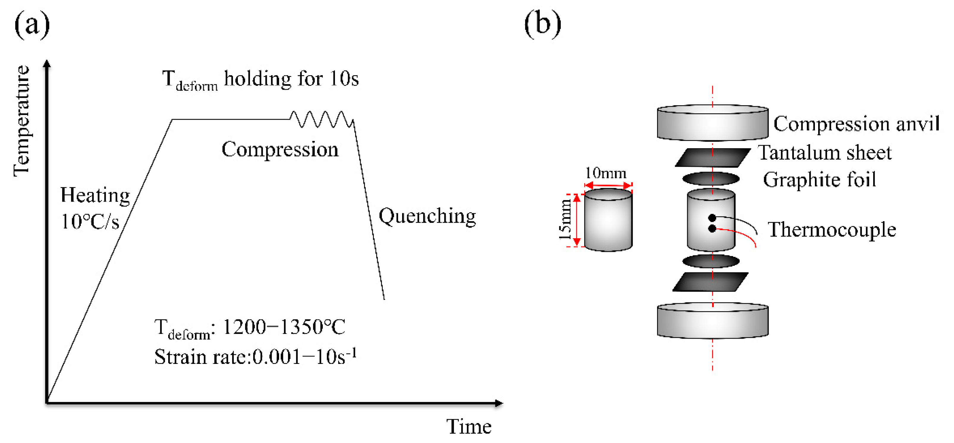
The samples were heated to the deformation temperature at a rate of 10 °C/s. After holding for 10 s, the samples were isothermally compressed and subsequently quenched by argon, as shown in Figure 1a. The samples were subjected to hot compression deformation with a degree of deformation of 60% (9 mm).
A schematic illustration of the hot compression test is shown in Figure 1b. The size of experimental cylindrical compression samples was Φ10 mm × 15 mm. Both its surfaces and ends were mechanically polished to remove the surface oxidation layer. The hot compression test was conducted on a Gleeble-3500 (Data Science International, St. Paul, America), thermal-mechanical simulator system at five strain rates (0.001 s−1, 0.01 s−1, 0.1 s−1,1 s−1, and 10 s−1) and four temperatures (1200 °C, 1250 °C, 1300 °C, and 1350 °C) in an argon atmosphere. W30Mo70 material with a size of Φ19.3 mm × 7 mm was used as the compression anvil. Tantalum sheet, graphite foil, and nickel-based lubricant were employed to eliminate friction.
3. Experimental Results
3.1. The Flow Characteristics
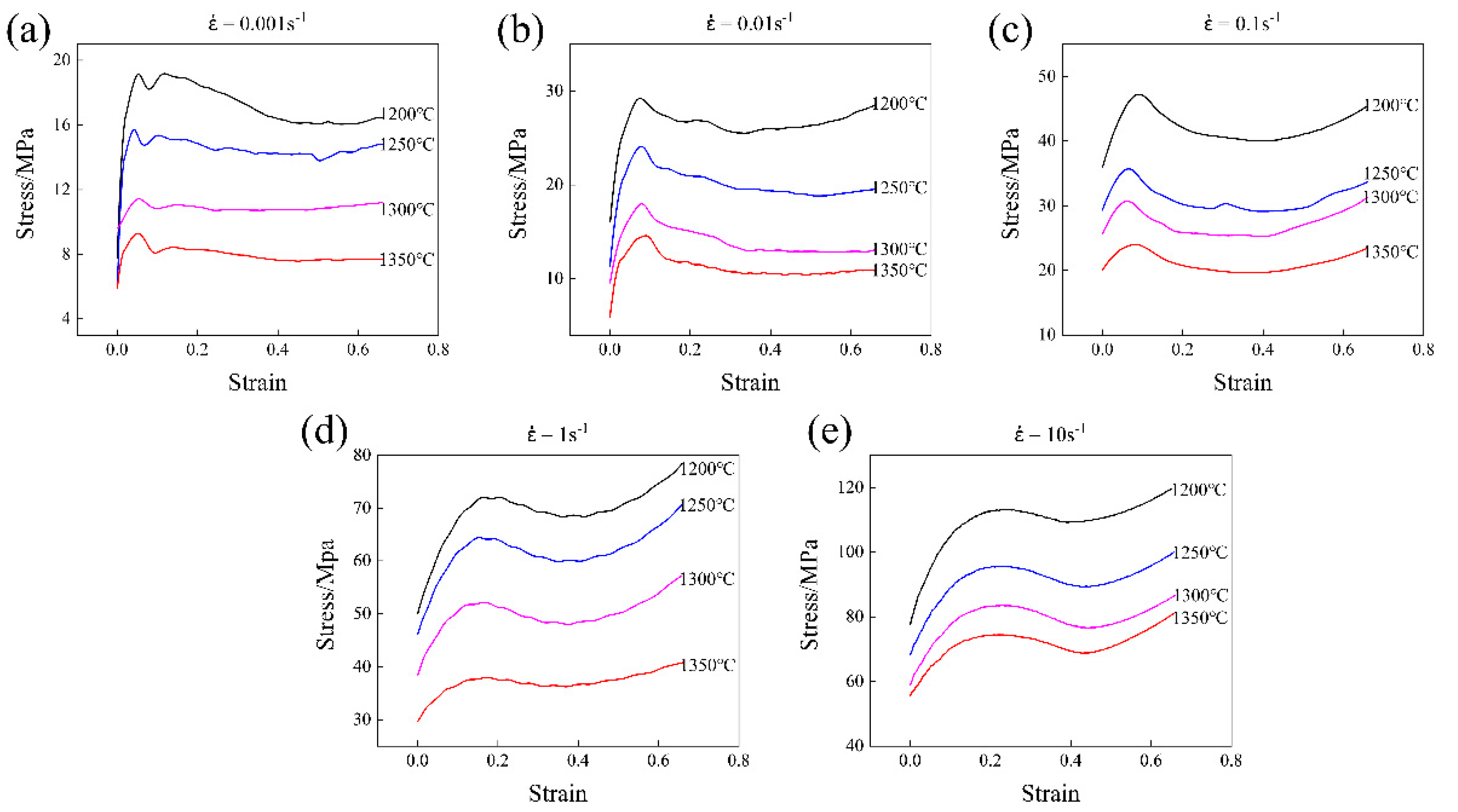
The stress–strain curve is corrected by friction according to Appendix A, and the results are shown in Figure 2. The stress decreases with increasing temperature and decreasing strain rate. At the same strain rate, the peak-strain decreases with the increase in temperature. At the same temperature, the peak-strain increases with the increase in strain rate.
There are two main characteristics of the curves:
- (1)
- The flow stress curves are divided into four stages according to the description of flow stress by Lin et al. [20]. In the initial stage (work hardening stage), with the increase in strain, stress increases as the work hardening rate is bigger than the softening rate. In the second stage (transition stage), the softening effect is gradually strengthened, causing a decrease in the stress increase rate, and thus the flow stress reaches its peak. In the third stage (softening stage), the flow softening effect caused by dynamic recovery (DRV) and DRX is greater than that caused by work hardening (WH), resulting in a rapid decrease in flow stress. In the fourth stage (steady stage), when the deformation reaches a specific value, the competition between WH and dynamic softening reaches a dynamic equilibrium. It is worth noting that when the strain rate is greater than 0.1 s−1, the stress has increased after reaching the steady state stage (), which is caused by friction
- (2)
- Flow stress curve changed from a single peak to multiple peaks when changed from 0.01 s−1 to 0.001 s−1.
The curves show a single peak at high strain rates () as the DRX rate is so slow that the first round of DRX is not completed when the second round of DRX has begun.
The curves show multiple peaks at a low strain rate (). According to our previous simulation results of the recrystallization process through the multiphase field method [23], the reason is that the second round of DRX takes place after the first round of DRX is completed.
The curve reaches its first peak due to the first round of DRX. The curve reach to its first trough due to growth of each new DRX grain. Then, the deformation is not over, and the dislocation density in the newly formed grains has not reached the critical density of dynamic recrystallization. Therefore, the grains undergo secondary WH, and the second work hardening peak appears. With the increase in dislocation density, the second dynamic recrystallization begins, forming a second trough. Such complex WH and softening of DRX superimposed alternately, and the curve periodically appears multiple peaks until equilibrium [24,25].
3.2. Constitutive Modeling the Flow Stress of 42CrMo
3.2.1. Arrhenius Constitutive Model
The derivation of strain-compensated Arrhenius constitutive equation is divided into two steps. The first step is to solve the Arrhenius constitutive equation under a specific strain to obtain the material parameters. The second step is to conduct polynomial fitting of material parameters under all strains to obtain the final equation.
- (1)
- Determination of material parameters
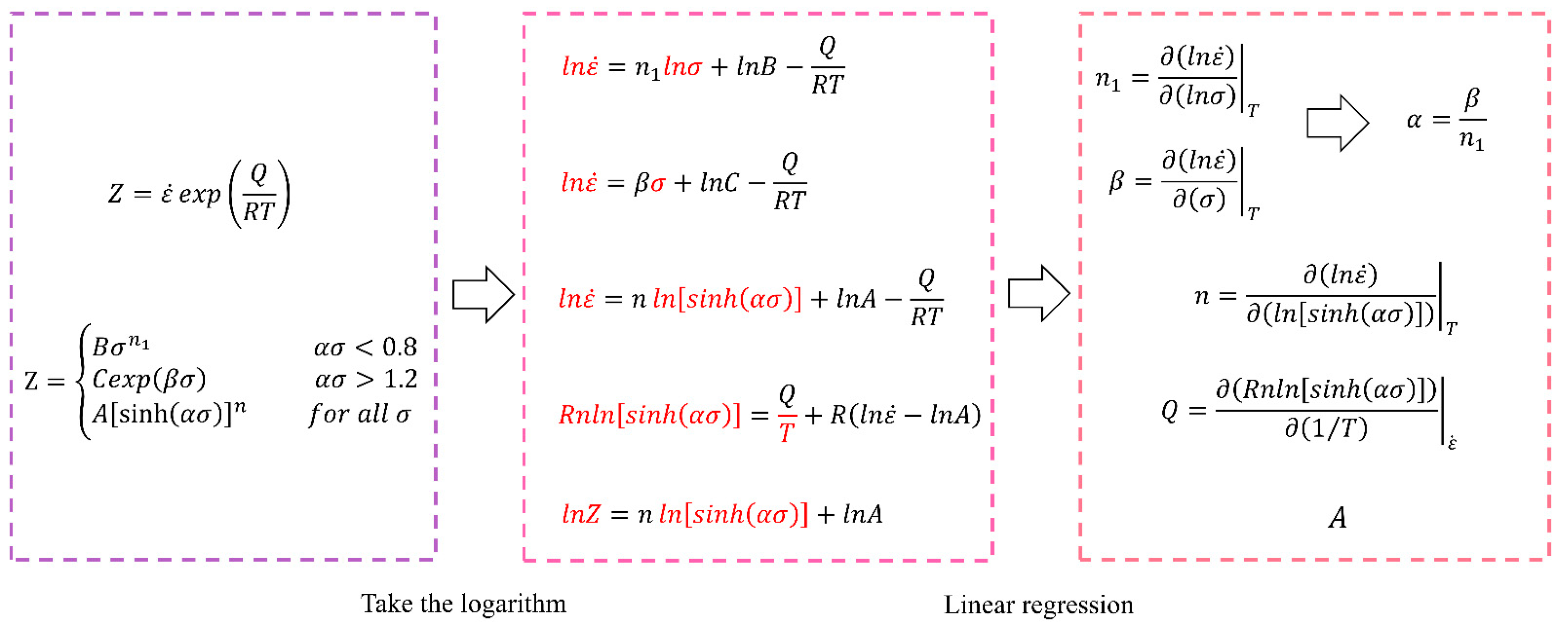
According to the Zener and Hollomon [26] research, stress is related to strain, temperature, and strain rate. The Arrhenius model has been widely used to describe the stress–strain relationship. The method of deriving material parameters from Z parameter is shown in Figure 3, and the formula derivation is shown in Appendix B.
- (2)
- Strain compensated constitutive equation
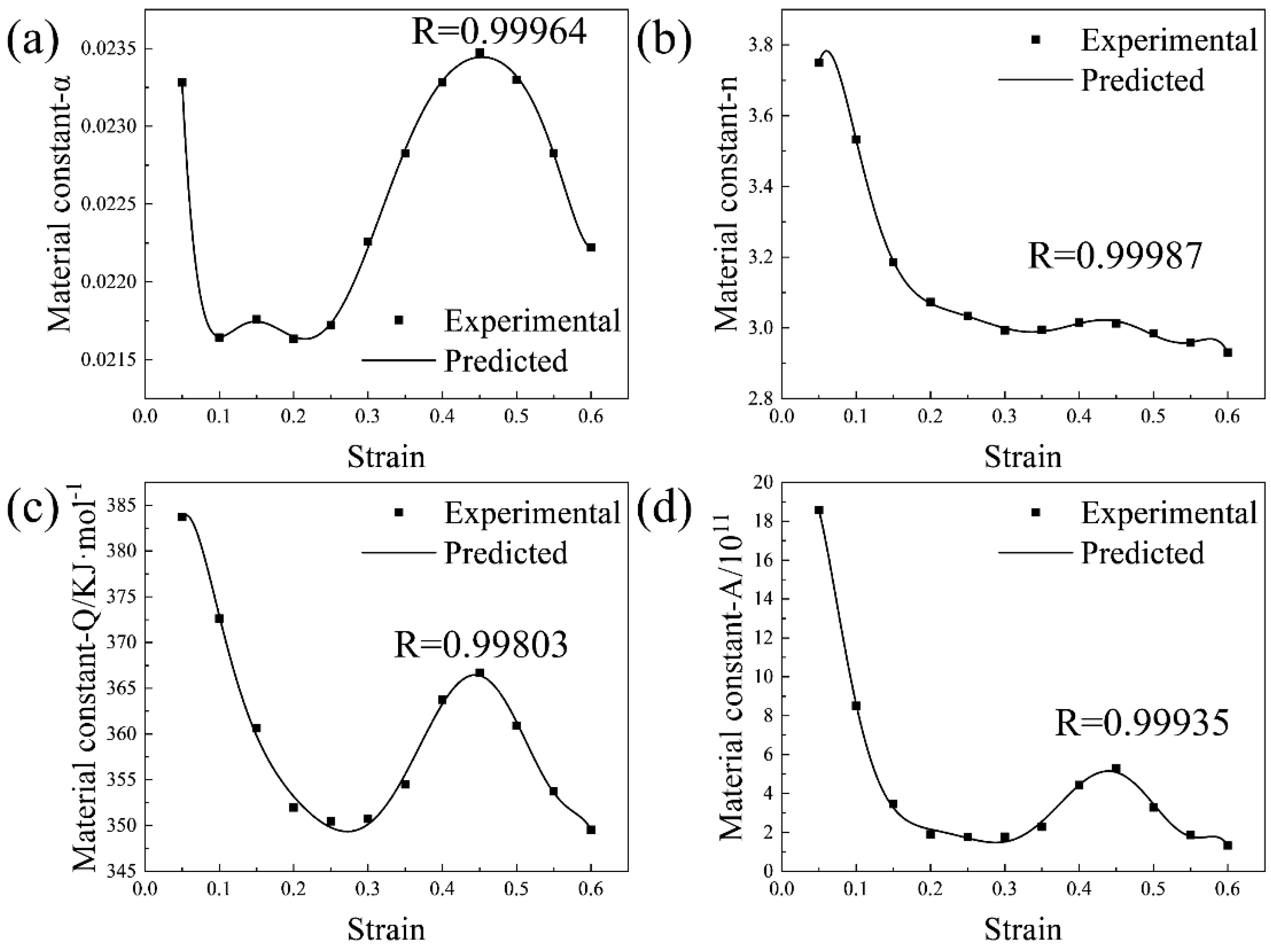
The parameters obtained by the above calculation and fitting process can only predict the flow stress under specific strain. Thus, the influence of strain on the flow stress must be considered. The effect of strain can be indirectly reflected on the material constants. The material constants of constitutive equations under different deformation strains are calculated at intervals of 0.05 in the range of 0.05–0.6. The relationship between strain and material constants (α, n, Q, and A) can be well fitted by a polynomial (Equation (1), m = 8). Figure 4 shows the fitting results, and the fitting coefficients of polynomials are shown in Table 2.
Some research [27,28] shows that the Arrhenius-type constitutive equation has a large error between the predicted and actual values at high temperatures and low strain rates. Therefore, a strain rate correction of Z parameter is carried out, and the equation is as follows [29]:
Strain compensated Arrhenius constitutive model can be expressed by Equation (3).
3.2.2. Back Propagation Artificial Neural Network Constitutive Model
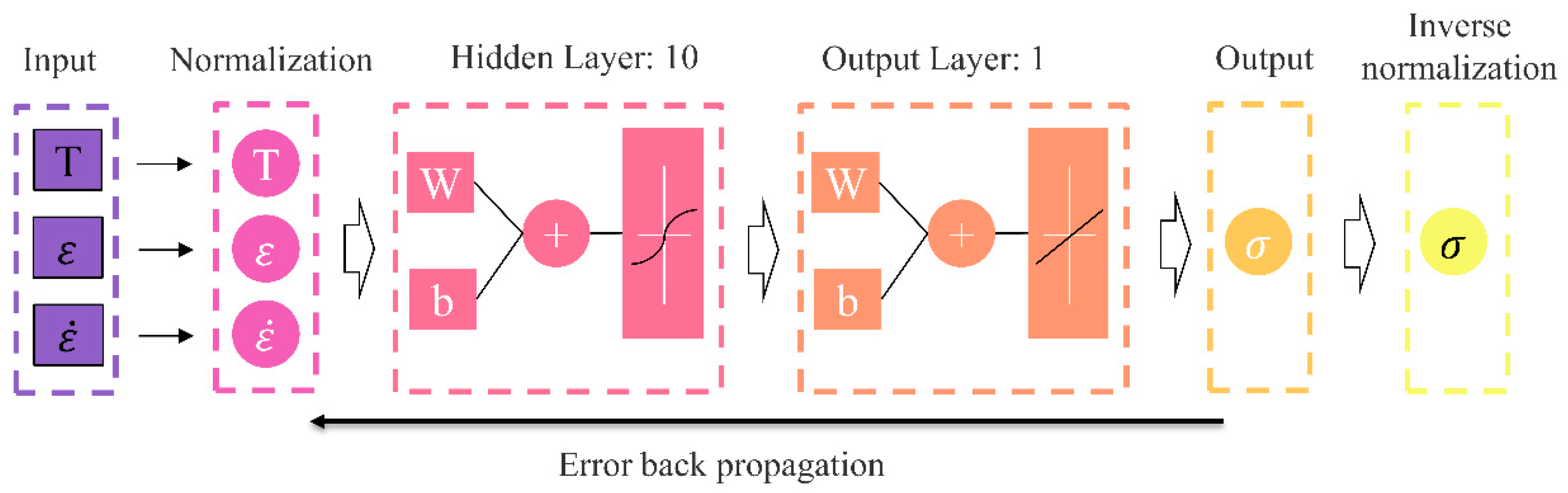
The back propagation artificial neural network constitutive (BP ANN) has been an excellent solution for complex nonlinear problems [30]. To better describe the flow stress of 42CrMo, the BP ANN model was employed in this research. A typical ANN consists of three units connected by weight values, namely, input layer, output layer, and hidden layer.
The ANN model with three input neurons, T, , and , and one output neuron, , is shown in Figure 5. The learning process of the BP ANN model is to continuously adjust the weights of neurons through error back propagation process. Neurons are equivalent to material parameters in conventional fitting methods, and weights are equivalent to parameter coefficients. The hidden layer contains 10 neurons. A logistic sigmoid function was employed as the activation function. The learning is based on the Levenberg–Marquardt algorithm. The learning rate is set as 0.001. The mean square error (MSE) was selected as the training objective function. MSE is expressed as Equation (4). Before training, all data need to be normalized in the [−1, 1] interval according to Equation (5).
where and are experimental and predicted values, respectively.
where is the original data, is the normalized data, and and are the maximum and minimum values of X, respectively.
3.2.3. Performance Evaluation of Constitutive Models
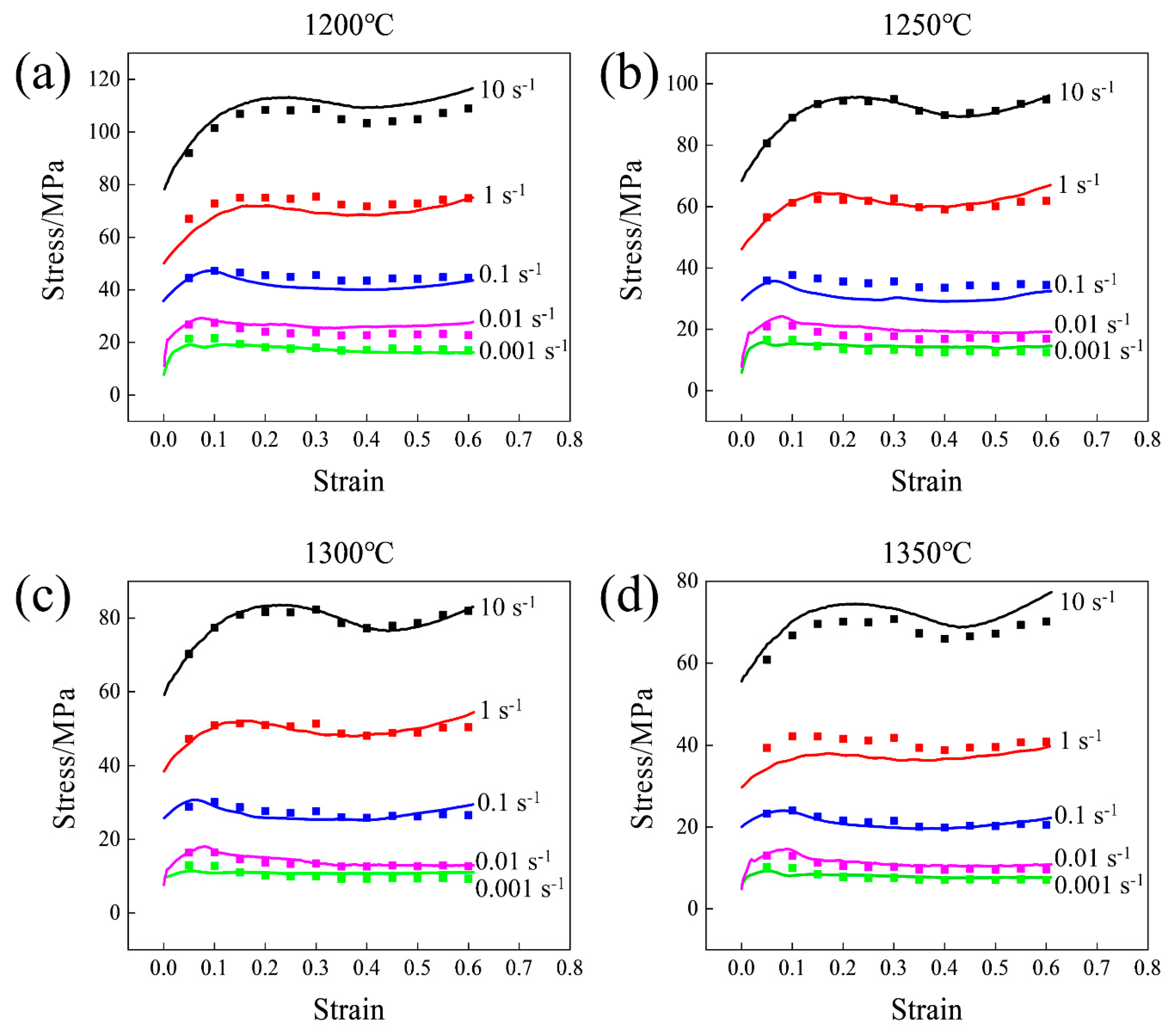
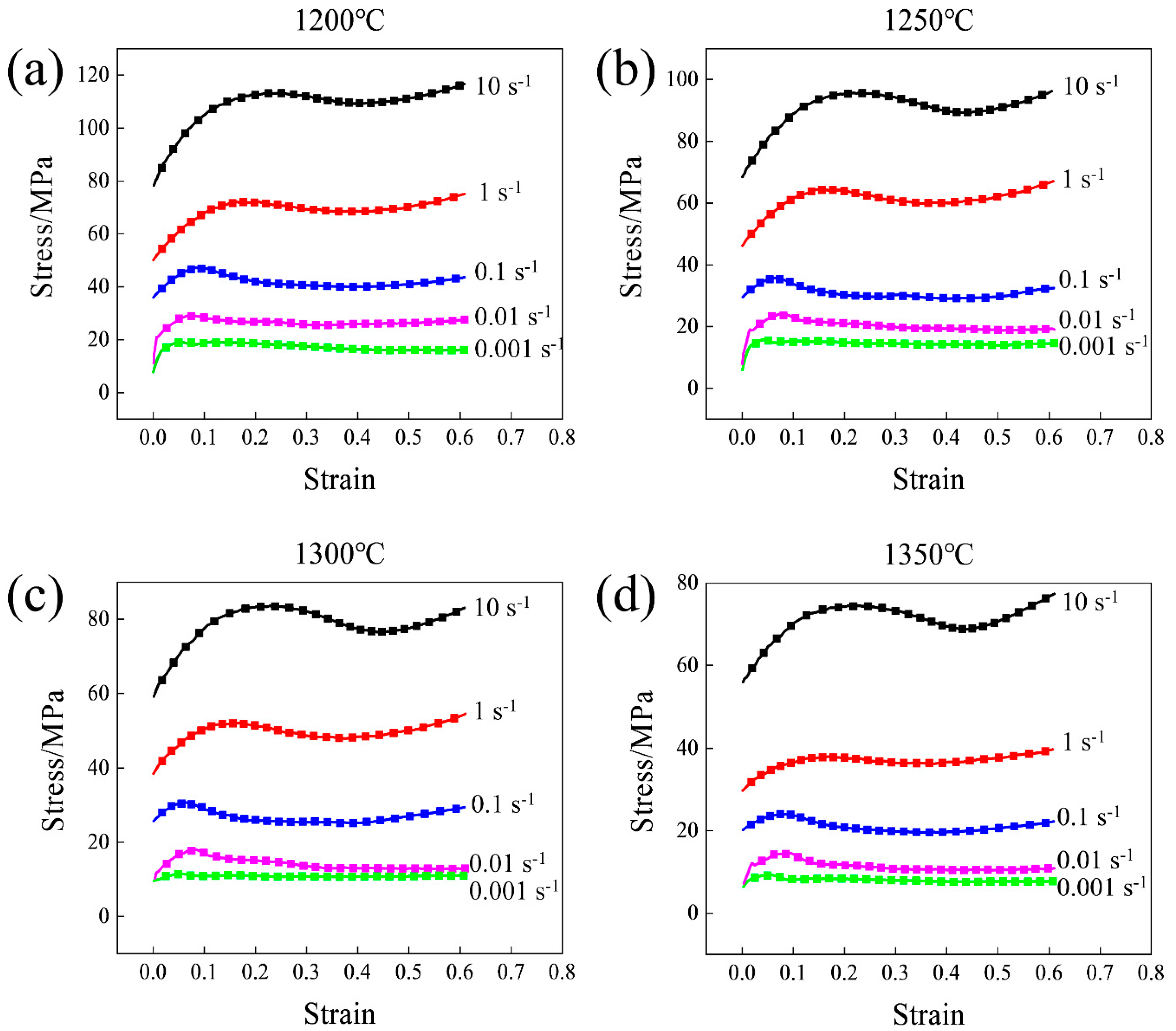
In this work, two models, i.e., the Arrhenius model and the BP ANN model, were employed to predict the strain-stress of 42CrMo at elevated temperatures. The comparison of experimental and predicted data from different models is shown in Figure 6 and Figure 7, respectively.
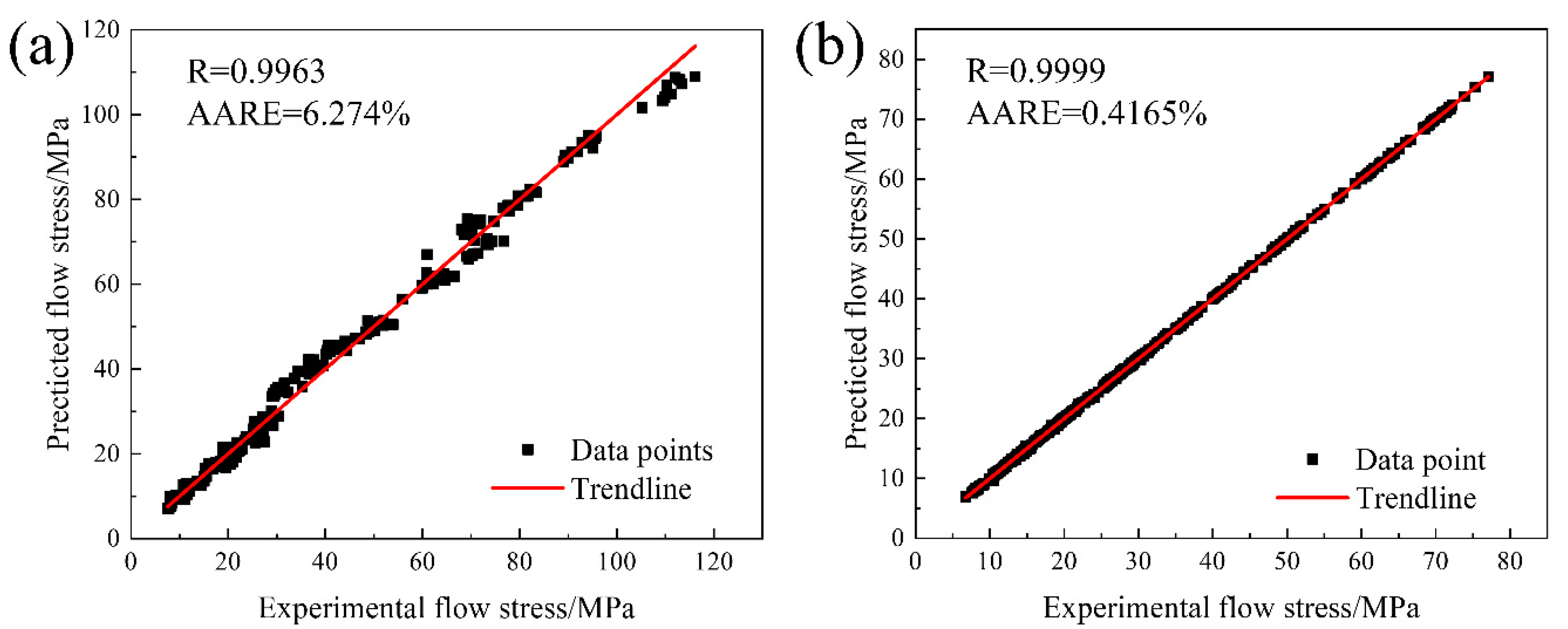
To quantitatively evaluate the performance of the above models, the R-value and average absolute relative error (AARE) value [4] are calculated by Equations (6) and (7), and the results are shown in Figure 8. The closer the R-value is to 1, the stronger the predictive ability is. The smaller the AARE value, the stronger the reliability of the prediction is [31].
where and are the experimental and predicted data, respectively, and E and P are the mean value.
It can be seen from Figure 6 and Figure 7 that the Arrhenius model has poor fitting results at large strain rates, while the BP ANN model has a better predictive ability. The R-value and AARE value of the BP ANN model are calculated to be 0.9999 and 0.4165%, respectively (Figure 8b), which are both lower than those of the strain-compensated Arrhenius model (Figure 8a), indicating that the BP ANN model has higher prediction accuracy and stability.
3.3. Hot Processing Maps
3.3.1. Hot Processing Maps Principles
To further clarify the DRX, DRV, and flow instability behavior of 42CrMo, the hot processing map was drawn according to the dynamic materials model (DMM) [32,33]. DMM defines that the total power of the input system, P, consists of two parts, namely the dissipation coordination J, and the dissipation G. Their relationship is Equation (8).
G and J represent the energy consumed by plastic deformation and by microstructure evolution, respectively. Strain rate sensitivity coefficient m decided their percent of P and can be expressed as.
J takes the maximum value Jmax when m = 1 under the ideal linear dissipation process. The energy consumption efficiency factor is defined as the ratio of the dissipation coefficient J to the ideal dissipation coefficient Jmax [34]. In general, the larger the η value is, the larger the energy proportion consumed by structural transformation is, and the better the working performance is. When drawing the thermal processing map, the instability region should also be avoided. Based on the maximum rate of entropy principle, the Prasad criterion was used to describe the flow instabilities (see Equation (11)).
3.3.2. Hot Processing Maps of 42CrMo
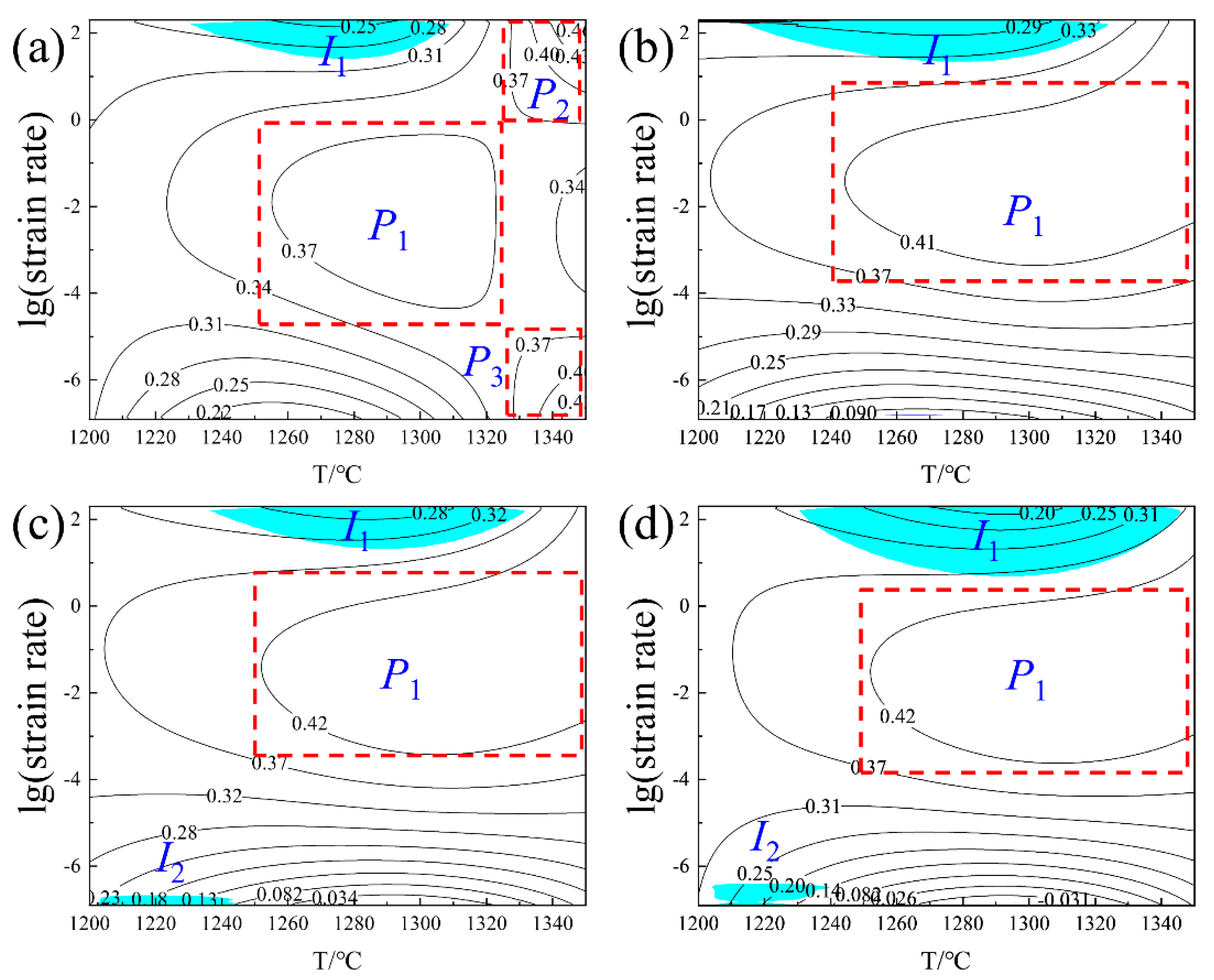
Figure 9 shows the processing maps of 42CrMo under different true strains. The contour lines represent the value of and the blue regions denote the flow instability. It is reported that a high value of indicates that the microstructure consumes more energy, and DRV, DRX, or phase transition may occur [35]. The regions of high values, which facilitate hot working, are marked with red lines. These regions are mainly distributed in the range of strain rate 0.01–1 s−1 and temperature greater than 1250 °C. Liu et al. [23] studied the dynamic recrystallization of the HR process by the multi-phase field method and found that a low strain rate promoted dynamic recrystallization, which could explain the areas where high values occur.
3.4. Dynamic Recrystallization Grain Analysis
3.4.1. Temperature Effect
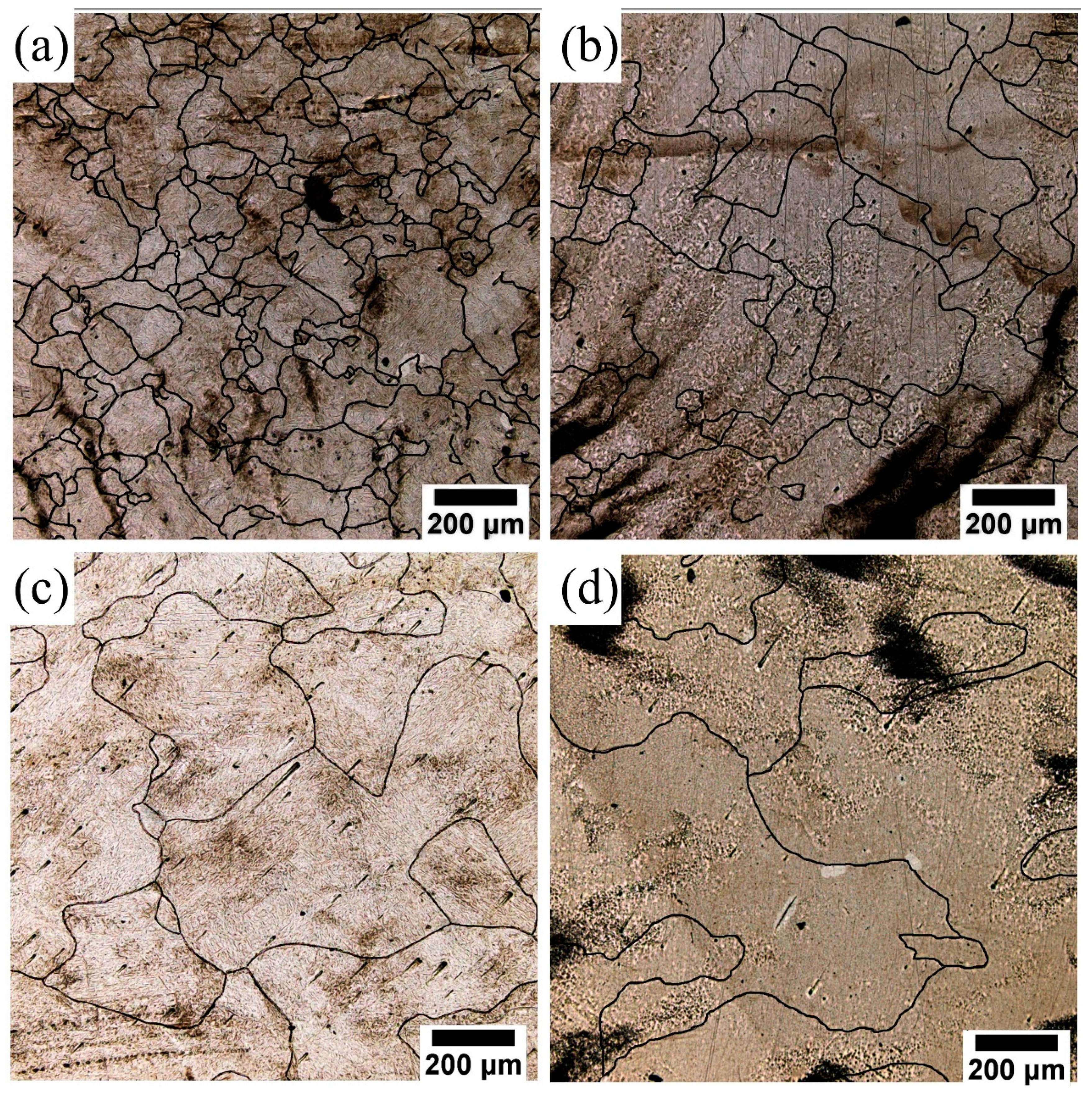
The samples were eroded in a supersaturated picric acid solution for an optical microscope (OM) observation to study the prior austenite grain boundaries. Deformation temperature affects recrystallized grains size. Figure 10 shows the prior austenite microstructure results at different temperatures under strain rate 0.01 s−1. The statistical results of Figure 10a–d are ~72 μm, ~112 μm, ~224 μm, and ~295 μm, respectively. High deformation temperature promotes grain boundary migration and increases grain size. The original grain was compressed along the deformation direction and elongated along the radial direction. Moreover, the deformed large grains are surrounded by newly generated DRX small grains, and the microstructure presents the characteristics of coexistence of original grains and recrystallization grains.
3.4.2. Strain Rate Effect
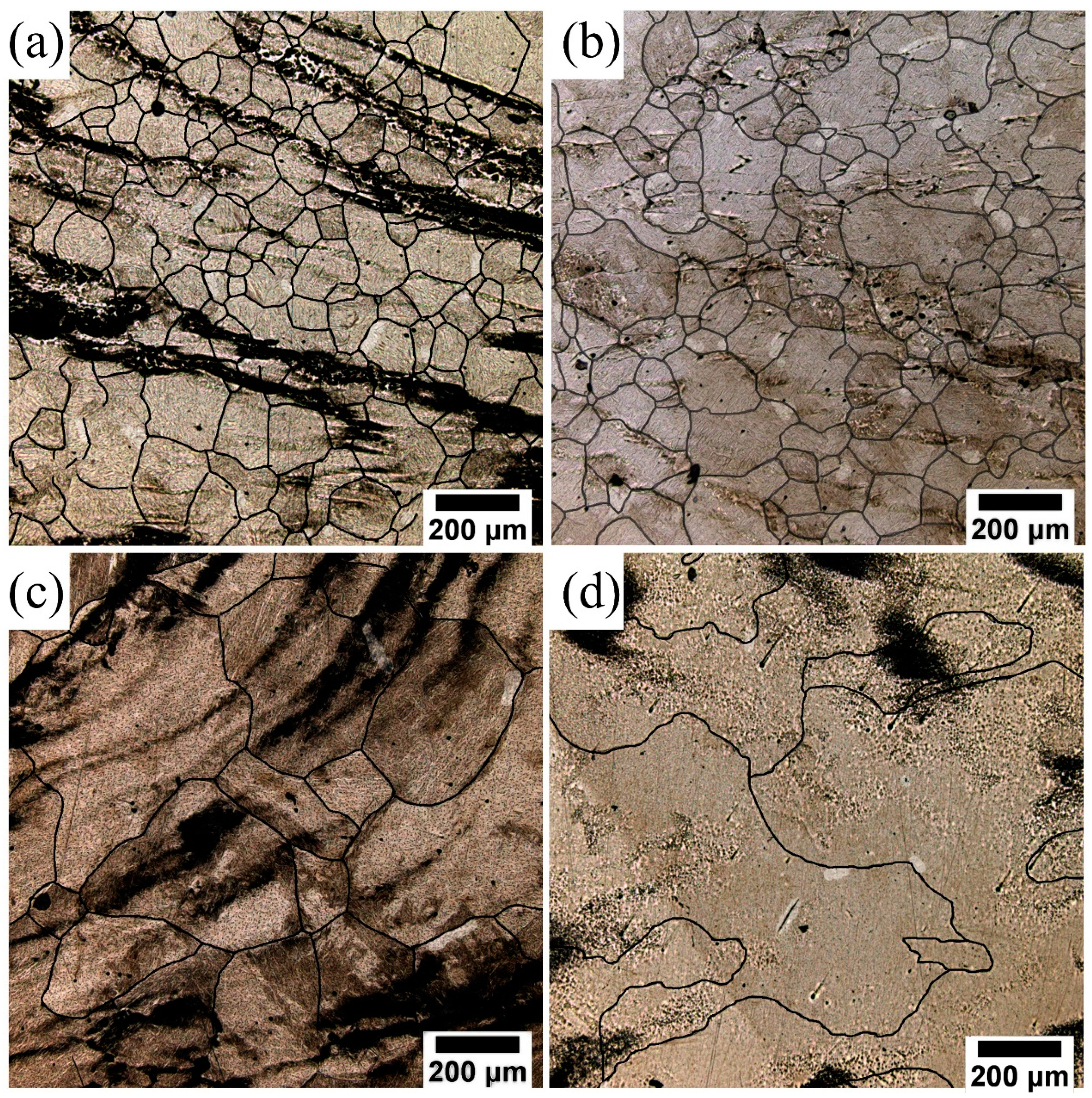
The strain rate also affects the recrystallized grains. Figure 11 shows the prior austenite microstructure results at different strain rates under 1350 °C. The statistical results of Figure 11a–d are ~60 μm, ~83 μm, ~183 μm, and ~295 μm, respectively. A large strain rate means large dislocation density and high deformation energy, which drives recrystallization. At the same time, a large strain rate means short recrystallization time, which hinders the subsequent recrystallization grain growth.
3.4.3. Grain Size Prediction Model
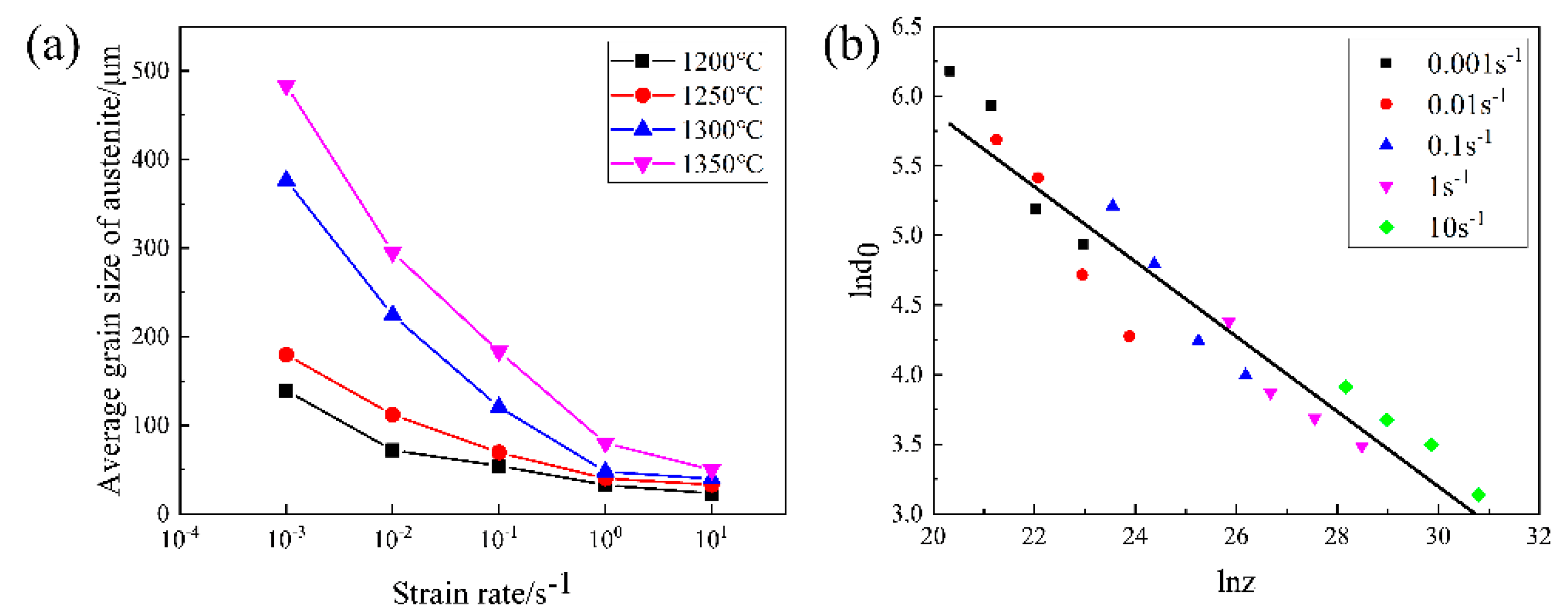
The average grain sizes of austenite at different strain rates were counted and shown in Figure 12a. The grain size decreases with the increase in strain rate at a specific temperature. Additionally, the grain size decreases with the decrease in temperature at a specific strain rate. The empirical equation can fit the relationship between austenite grain size and Z parameter . The fitting equation is shown in Equation (12), and the fitting curve is shown in Figure 12b.
4. Conclusions
- The flow stress of 42CrMo steel during hot compression deformation is mainly characterized by WH and a high temperature softening mechanism. The flow stress decreases with increasing temperatures and decreasing strain rates.
- Based on the strain compensation Arrhenius constitutive equation, the constitutive equation of 42CrMo steel at 1200–1350 °C and 0.01–10 s−1 was established. The mathematical form is
- 3.
- A single hidden layer BP ANN model with 10 hidden neurons was established to predict the flow behavior of 42CrMo, and the results showed that the BP ANN model has higher accuracy and stability to predict the curve than the Arrhenius model.
- 4.
- Based on the analysis of the thermal processing map, the optimal high reduction process parameter range of 42CrMo is obtained: the temperature range is 1250–1350 °C, and the strain rate range is 0.01–1 s−1.
Author Contributions
Conceptualization, W.Y. and Q.C.; methodology, W.Y.; software, J.Z. and G.W.; validation, H.L.; data curation, H.L.; writing—original draft preparation, H.L.; writing—review and editing, H.L. and Z.C. All authors have read and agreed to the published version of the manuscript.
Funding
This research received no external funding.
Institutional Review Board Statement
Not applicable.
Informed Consent Statement
Not applicable.
Conflicts of Interest
The authors declare no conflict of interest.
Appendix A. Friction Correction
In the metal forming process, friction affects a tools’ life cycle, the formability of workpiece material, and product quality. Friction increases the uneven deformation, resulting in fluctuations in the curve in hot compression process. Researchers reduce the harmful effects of friction by employing nickel-based lubricants and graphite sheets in hot compression experiments. However, the influence of friction increased with the increase in strain, and the phenomenon of ‘bulging’ would appear. Li et al. [36] analyzed friction coefficient evolution under large strain in the hot forging process and found that the friction coefficient was constant at low strain levels and exponential at high strain levels. Therefore, the measured flow stress needs to be corrected by the friction correction method proposed in previous research [37,38,39].
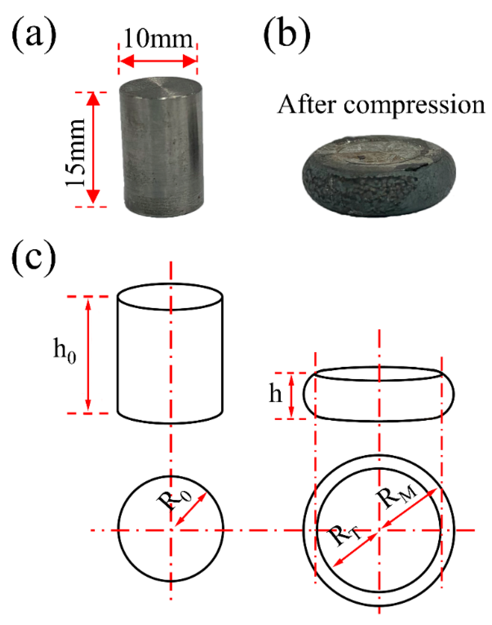
A simple representation of hot compression test is presented in Figure A1. The parameters, including initial radius R0, maximum radius RM, initial height h0, and final height h, can be directly measured, as shown in Figure A1c. The transformation from the measured stress to the corrected stress can be obtained from the following equation [36]:
where and are the corrected and measured flow stress, respectively, and is the correction coefficient, which could be evaluated by Equation (A2).
![Metals 11 01614 g0a1]() where R is the theoretical radius, which can be evaluated by Equation (A3) and m is the average friction coefficient of the entire working process varying from 0 (perfect sliding) to 1 (sticking), which can be evaluated by Equation (A4) [39].
where b is the barreling factor, which can be evaluated by Equation (A5).
where is the difference between the maximum radius RM and the top radius RT of the sample, respectively, which can be evaluated by Equations (A6) and (A7), respectively, and is the height difference before and after sample compression, which can be evaluated by Equation (A8).
where R is the theoretical radius, which can be evaluated by Equation (A3) and m is the average friction coefficient of the entire working process varying from 0 (perfect sliding) to 1 (sticking), which can be evaluated by Equation (A4) [39].
where b is the barreling factor, which can be evaluated by Equation (A5).
where is the difference between the maximum radius RM and the top radius RT of the sample, respectively, which can be evaluated by Equations (A6) and (A7), respectively, and is the height difference before and after sample compression, which can be evaluated by Equation (A8).
Figure A1.
Diagram of samples shape before (a) and after (b) hot compression, and (c) relevant parameters in friction correction.
Figure A1.
Diagram of samples shape before (a) and after (b) hot compression, and (c) relevant parameters in friction correction.

Appendix B. Derivation of Arrhenius Constitutive Equation
Under different stress states, Z parameter can be expressed as Equations (A9) and (A10) [21,40].
where Z is strain rate compensation factor; is strain rate; Q is deformation activation energy; R is gas constant; and T is deformation temperature.
where A, B, C, α, β, n1, and n are material constants.
The following formula can be obtained by taking logarithms on both sides of Equations (A9) and (A10), respectively.
The following parameters can be obtained by linear fitting from Equation (A11). Additionally, lnA was determined from the intercept of the lnZ-ln [sinh(ασ)] line.
References
- Zhang, J.; Liu, Z.; Sun, J.; Zhao, H.; Shi, Q.; Ma, D. Microstructure and mechanical property of electropulsing tempered ultrafine grained 42CrMo steel. Mater. Sci. Eng. A 2020, 782, 139213. [Google Scholar] [CrossRef]
- Li, Y.; Wang, Z.; Zhang, L.; Luo, C.; Lai, X. Arrhenius-Type Constitutive Model and Dynamic Recrystallization Behavior of V–5Cr–5Ti Alloy during Hot Compression. Trans. Nonferrous Met. Soc. China 2015, 25, 1889–1900. [Google Scholar] [CrossRef]
- Liu, G.; Zhang, D.; Yao, C. A Modified Constitutive Model Coupled with Microstructure Evolution Incremental Model for Machining of Titanium Alloy Ti–6Al–4V. J. Mater. Process. Technol. 2021, 297, 117262. [Google Scholar] [CrossRef]
- Yao, C.; Wang, B.; Yi, D.; Wang, B.; Ding, X. Artificial neural network modelling to predict hot deformation behaviour of as HIPed FGH4169 superalloy. Mater. Sci. Technol. 2014, 30, 1170–1176. [Google Scholar] [CrossRef]
- Lin, Y.C.; Zhang, J.; Zhong, J. Application of neural networks to predict the elevated temperature flow behavior of a low alloy steel. Comput. Mater. Sci. 2008, 43, 752–758. [Google Scholar] [CrossRef]
- Yu, R.; Li, X.; Li, W.; Chen, J.; Guo, X.; Li, J. Application of four different models for predicting the high-temperature flow behavior of TG6 titanium alloy. Mater. Today Commun. 2021, 26, 102004. [Google Scholar] [CrossRef]
- Stoian, E.V.; Bratu, V.; Enescu, C.M.; Rusanescu, C.O. Analysis of Internal Defects Appeared in the Continuous Casting. Sci. Bull. Valahia Univ. Mater. Mech. 2018, 16, 23–27. [Google Scholar] [CrossRef] [Green Version]
- Ali, N.; Zhang, L.; Zhou, H.; Zhao, A.; Zhang, C.; Fu, K.; Cheng, J. Effect of Soft Reduction Technique on Microstructure and Toughness of Medium Carbon Steel. Mater. Today Commun. 2021, 26, 102130. [Google Scholar] [CrossRef]
- Chu, R.; Li, Z.; Liu, J.; Fan, Y.; Liu, Y.; Ma, C. Effect of Soft Reduction Process on Segregation of a 400 mm Thick High-alloy Steel Slab. J. Iron Steel Res. Int. 2021, 28, 272–278. [Google Scholar] [CrossRef]
- Ning, Z.; Yu, W.; Liu, H.; Cai, Q. Effect of Reduction Pretreatment Process on Evolution of Micro-porosity in 42CrMo Billet. J. Iron Steel Res. Int. 2021, 28, 413–423. [Google Scholar] [CrossRef]
- Liu, H.; Cheng, Z.; Yu, W.; Zhou, Z.; Cheng, L.; Cai, Q. Effect of High-temperature Reduction Pretreatment on Internal Quality of 42CrMo Casting Billet. J. Iron Steel Res. Int. 2021, 28, 693–702. [Google Scholar] [CrossRef]
- Wang, Y.; Cai, Q.; Li, G.; Yu, W. Effects of Reduction Pretreatment on the Internal Quality of Casting Billets. Steel Res. Int. 2017, 88. [Google Scholar] [CrossRef]
- Liu, H.; Cheng, Z.; Yu, W.; Cai, Q. Recrystallization and Diffusion Mechanisms of Segregation Improvement in Cast Billets by High Temperature Reduction Pretreatment. Mater. Res. Express 2021, 8, 046539. [Google Scholar] [CrossRef]
- Kawamoto, M. Recent Development of Steelmaking Process in Sumitomo Metals. J. Iron Steel Res. Int. 2011, 18, 28–35. [Google Scholar] [CrossRef]
- Seiji, N.; Hakaru, N.; Tetsuya, F.; Tohsio, F.; Koichi, K.; Hisakazu, M. Control of Centerline Segregation in Continuously Cast Blooms by Continuous Forging Process. ISIJ Int. 1995, 35, 673–679. [Google Scholar] [CrossRef] [Green Version]
- Takubo, M.; Matsuoka, Y.; Miura, Y.; Higashi, H.; Kittaka, S. NSENGI’s New Developed Bloom Continuous Casting Technology for Improving Internal Quality of Special Bar Quality(NS Bloom Large Reduction). In Proceedings of the Symposium on Technology Innovation and Fine Production of Continuous Casting Equipment Meeting, Xi’an, China, 17 June 2015; pp. 307–318. [Google Scholar]
- Li, H.; Gong, M.; Li, T.; Wang, Z.; Wang, G. Effects of Hot-Core Heavy Reduction Rolling during Continuous Casting on Microstructures and Mechanical Properties of Hot-Rolled Plates. J. Mater. Process. Technol. 2020, 283, 116708. [Google Scholar] [CrossRef]
- Li, G.; Yu, W.; Cai, Q. Investigation of Reduction Pretreatment Process for Continuous Casting. J. Mater. Process. Technol. 2016, 227, 41–48. [Google Scholar] [CrossRef]
- Ji, C.; Wu, C.; Zhu, M. Thermo-Mechanical Behavior of the Continuous Casting Bloom in the Heavy Reduction Process. JOM 2016, 68, 3107–3115. [Google Scholar] [CrossRef] [Green Version]
- Lin, Y.; Chen, M.; Zhong, J. Prediction of 42CrMo Steel Flow Stress at High Temperature and Strain Rate. Mech. Res. Commun. 2008, 35, 142–150. [Google Scholar] [CrossRef]
- Ji, H.; Duan, H.; Li, Y.; Li, W.; Huang, X.; Pei, W.; Lu, Y. Optimization the working parameters of as-forged 42CrMo steel by constitutive equation-dynamic recrystallization equation and processing maps. J. Mater. Res. Technol. 2020, 9, 7210–7224. [Google Scholar] [CrossRef]
- Duan, H.; Huang, X.; Ji, H.; Li, Y. The Arrhenius constitutive model of steel 42CrMo for gear. Metalurgija 2020, 59, 63–66. [Google Scholar]
- Liu, H.; Ning, Z.; Yu, W.; Cheng, Z.; Wang, X.; Cai, Q. Dynamic Recrystallization Analysis of Reduction Pretreatment Process by Multi-Phase Field Method. Mater. Res. Express 2020, 7, 106501. [Google Scholar] [CrossRef]
- Sakai, T.; Belyakov, A.; Kaibyshev, R.; Miura, H.; Jonas, J.J. Dynamic and Post-Dynamic Recrystallization under Hot, Cold and Severe Plastic Deformation Conditions. Prog. Mater. Sci. 2014, 60, 130–207. [Google Scholar] [CrossRef] [Green Version]
- Sakai, T.; Jonas, J.J. Plastic Deformation: Role of Recovery and Recrystallization. In Encyclopedia of Materials: Science and Technology; Buschow, K.H.J., Cahn, R.W., Flemings, M.C., Ilschner, B., Kramer, E.J., Mahajan, S., Veyssière, P., Eds.; Elsevier: Oxford, UK, 2001; pp. 7079–7084. [Google Scholar] [CrossRef]
- Zener, C.; Hollomon, J.H. Effect of strain rate upon plastic flow of steel. J. Appl. Phys. 1944, 15, 22–32. [Google Scholar] [CrossRef]
- He, A.; Chen, L.; Hu, S.; Wang, C.; Huangfu, L. Constitutive analysis to predict high temperature flow stress in 20CrMo continuous casting billet. Mater. Des. 2013, 46, 54–60. [Google Scholar] [CrossRef]
- Cai, J.; Li, F.; Liu, T.; Chen, B.; He, M. Constitutive equations for elevated temperature flow stress of Ti–6Al–4V alloy considering the effect of strain. Mater. Des. 2011, 32, 1144–1151. [Google Scholar] [CrossRef]
- Lin, Y.; Chen, M.; Zhong, J. Constitutive modeling for elevated temperature flow behavior of 42CrMo steel. Comput. Mater. Ence 2008, 42, 470–477. [Google Scholar] [CrossRef]
- Murugesan, M.; Jung, D.W. Back Propagation Artificial Neural Network Approach to Predict the Flow Stress in Isothermal Tensile Test of Medium Carbon Steel Material. In Proceedings of the Materials Science Forum, Jeju Island, Korea, 30–31 July 2020; pp. 163–168. [Google Scholar]
- Zhu, Y.; Cao, Y.; Liu, C.; Luo, R.; Li, N.; Shu, G.; Huang, G.; Liu, Q. Dynamic behavior and modified artificial neural network model for predicting flow stress during hot deformation of Alloy 925. Mater. Today Commun. 2020, 25, 101329. [Google Scholar] [CrossRef]
- Prasad, Y. Author’s reply: Dynamic materials model: Basis and principles. Metall. Mater. Trans. A 1996, 27, 235–236. [Google Scholar] [CrossRef]
- Prasad, Y.V.R.K.; Seshacharyulu, T. Modelling of hot deformation for microstructural control. Int. Mater. Rev. 1998, 43, 243–258. [Google Scholar] [CrossRef]
- Dong, Y.; Zhang, C.; Zhao, G.; Guan, Y.; Gao, A.; Sun, W. Constitutive equation and processing maps of an Al–Mg–Si aluminum alloy: Determination and application in simulating extrusion process of complex profiles. Mater. Des. 2016, 92, 983–997. [Google Scholar] [CrossRef]
- Yang, Z.; Zhang, F.; Zheng, C.; Zhang, M.; Lv, B.; Qu, L. Study on hot deformation behaviour and processing maps of low carbon bainitic steel. Mater. Des. 2015, 66, 258–266. [Google Scholar] [CrossRef]
- Li, Y.; Onodera, E.; Matsumoto, H.; Chiba, A. Correcting the Stress-Strain Curve in Hot Compression Process to High Strain Level. Metall. Mater. Trans. A 2009, 40, 982–990. [Google Scholar] [CrossRef] [Green Version]
- Ebrahimi, R.; Najafizadeh, A. A New Method For Evaluation of Friction in Bulk Metal Forming. J. Mater. Process. Technol. 2004, 152, 136–143. [Google Scholar] [CrossRef]
- Lin, Y.; Xia, Y.; Chen, X.; Chen, M. Constitutive Descriptions for Hot Compressed 2124-T851 Aluminum Alloy over a Wide Range of Temperature and Strain Rate. Comput. Mater. Sci. 2010, 50, 227–233. [Google Scholar] [CrossRef]
- Li, Y.; Onodera, E.; Chiba, A. Friction Coefficient in Hot Compression of Cylindrical Sample. Mater. Trans. 2010, 51, 1210–1215. [Google Scholar] [CrossRef] [Green Version]
- Wei, T.; Wang, Y.; Tang, Z.; Xiao, S. The constitutive modeling and processing map of homogenized Al-Mg-Si-Cu-Zn alloy. Mater. Today Commun. 2021, 27, 102471. [Google Scholar] [CrossRef]
Figure 1.
(a) Hot compression experiment procedure diagram and (b) schematic illustration of the hot compression test.
Figure 1.
(a) Hot compression experiment procedure diagram and (b) schematic illustration of the hot compression test.

Figure 2.
True−stress/true−strain curve of 42CrMo steel after friction correction under different deformation conditions: (a) 0.001 s−1; (b) 0.01 s−1; (c) 0.1 s−1; (d) 1 s−1; and (e) 10 s−1.
Figure 2.
True−stress/true−strain curve of 42CrMo steel after friction correction under different deformation conditions: (a) 0.001 s−1; (b) 0.01 s−1; (c) 0.1 s−1; (d) 1 s−1; and (e) 10 s−1.

Figure 3.
Flow chart of Arrhenius constitutive model parameters solving.

Figure 4.
Linear fitting schematic between strain and material constants α (a), n (b), Q (c), and A (d).
Figure 4.
Linear fitting schematic between strain and material constants α (a), n (b), Q (c), and A (d).

Figure 5.
Schematic of the BP ANN with a single hidden layer.

Figure 6.
Predicted and experimental data of flow stress from Arrhenius model at various strain rates and temperatures: (a) 1200 °C; (b) 1250 °C; (c) 1300 °C; (d) 1350 °C.
Figure 6.
Predicted and experimental data of flow stress from Arrhenius model at various strain rates and temperatures: (a) 1200 °C; (b) 1250 °C; (c) 1300 °C; (d) 1350 °C.

Figure 7.
Predicted and experimental data of flow stress from BP ANN model at various strain rates and temperatures: (a) 1200 °C; (b) 1250 °C; (c) 1300 °C; (d) 1350 °C.
Figure 7.
Predicted and experimental data of flow stress from BP ANN model at various strain rates and temperatures: (a) 1200 °C; (b) 1250 °C; (c) 1300 °C; (d) 1350 °C.

Figure 8.
Comparison of predicted and experimental flow stress by (a) strain-compensated Arrhenius model and (b) BP ANN model.
Figure 8.
Comparison of predicted and experimental flow stress by (a) strain-compensated Arrhenius model and (b) BP ANN model.

Figure 9.
Hot processing maps under different true strains: (a) = 0.1; (b) = 0.2; (c) = 0.3; and (d) = 0.4.
Figure 9.
Hot processing maps under different true strains: (a) = 0.1; (b) = 0.2; (c) = 0.3; and (d) = 0.4.

Figure 10.
Austenite grain under strain rate 0.01 s−1 of (a) 1200 °C; (b) 1250 °C; (c) 1300 °C; and (d) 1350 °C.
Figure 10.
Austenite grain under strain rate 0.01 s−1 of (a) 1200 °C; (b) 1250 °C; (c) 1300 °C; and (d) 1350 °C.

Figure 11.
Austenite grain under temperature 1350 °C of (a) 10 s−1; (b) 1 s−1; (c) 0.1 s−1; and (d) 0.01 s−1.
Figure 11.
Austenite grain under temperature 1350 °C of (a) 10 s−1; (b) 1 s−1; (c) 0.1 s−1; and (d) 0.01 s−1.

Figure 12.
The relationship between d0 and Z parameters (a) statistical results of dynamic recrystallization grain size; (b) ln -lnZ.
Figure 12.
The relationship between d0 and Z parameters (a) statistical results of dynamic recrystallization grain size; (b) ln -lnZ.


Table 1.
Chemical composition of experimental 42CrMo steels (wt.%).
| C | Mn | Si | P | S | Ni | Cr | Mo | Ti | Fe |
|---|---|---|---|---|---|---|---|---|---|
| 0.39 | 0.72 | 0.24 | 0.014 | 0.005 | 0.009 | 1.12 | 0.189 | 0.0039 | Balance |
Table 2.
Coefficients of the polynomial for material constants α, n, Q, and A.
| Coefficient | α | n | A | Q |
|---|---|---|---|---|
| 0 | 0.03744 | 1.38678 | 5.99 × 10¹¹ | 314,383.9372 |
| 1 | −0.57203 | 111.8692 | 9.93 × 10¹³ | 3,500,920 |
| 2 | 8.36659 | −1919.02 | −2.37 × 10¹⁵ | −64,276,000 |
| 3 | −64.3572 | 15,697.7 | 2.30 × 10¹⁶ | 558,432,000 |
| 4 | 285.862 | −72,404.1 | −1.19 × 10¹⁷ | −2,752,800,000 |
| 5 | −756.918 | 198,419 | 3.54 × 10¹⁷ | 8,058,170,000 |
| 6 | 1180.568 | −320,115 | −6.08 × 10¹⁷ | −13,772,100,000 |
| 7 | −1002.47 | 280,571.3 | 5.59 × 10¹⁷ | 12,636,300,000 |
| 8 | 357.8014 | −102,991 | −2.12 × 10¹⁷ | −4,797,100,000 |
Publisher’s Note: MDPI stays neutral with regard to jurisdictional claims in published maps and institutional affiliations. |
© 2021 by the authors. Licensee MDPI, Basel, Switzerland. This article is an open access article distributed under the terms and conditions of the Creative Commons Attribution (CC BY) license (https://creativecommons.org/licenses/by/4.0/).
Share and Cite
MDPI and ACS Style
Liu, H.; Cheng, Z.; Yu, W.; Wang, G.; Zhou, J.; Cai, Q. Deformation Behavior and Constitutive Equation of 42CrMo Steel at High Temperature. Metals 2021, 11, 1614. https://doi.org/10.3390/met11101614
AMA Style
Liu H, Cheng Z, Yu W, Wang G, Zhou J, Cai Q. Deformation Behavior and Constitutive Equation of 42CrMo Steel at High Temperature. Metals. 2021; 11(10):1614. https://doi.org/10.3390/met11101614
Chicago/Turabian StyleLiu, Hongqiang, Zhicheng Cheng, Wei Yu, Gaotian Wang, Jie Zhou, and Qingwu Cai. 2021. "Deformation Behavior and Constitutive Equation of 42CrMo Steel at High Temperature" Metals 11, no. 10: 1614. https://doi.org/10.3390/met11101614
Note that from the first issue of 2016, this journal uses article numbers instead of page numbers. See further details here.