Detection of Corrosion-Indicating Oxidation Product Colors in Steel Bridges under Varying Illuminations, Shadows, and Wetting Conditions

Abstract

Early detection of corrosion in steel bridges is essential for strategizing the mitigation of further corrosion damage. Although various image-based approaches are available in the literature for corrosion detection, most of these approaches are tested on images acquired under uniform natural daylight illuminations i.e., inherent variations in the ambient lighting conditions are ignored. Owing to the fact that varying natural daylight illuminations, shadows, water wetting, and oil wetting are unavoidable in real-world scenarios, it is important to devise a robust technique for corrosion identification. In the current study, four different color spaces namely ‘RGB’, ‘rgb’, ‘HSV’ and ‘CIE La*b*’ along with a multi-layer perceptron (MLP) is configured and trained for detecting corrosion under above-mentioned real-world illumination scenarios. Training (5000 instances) and validation (2064 instances) datasets for this purpose are generated from the images of corroded steel plates acquired in the laboratory under varying illuminations and shadows, respectively. Each combination of color space and an MLP configuration is individually assessed and the best suitable combination that yields the highest ‘Recall’ value is determined. An MLP configuration with a single hidden layer consisting of 4 neurons (1st Hidden Layer (HL)(4N)) in conjunction with ‘rgb’ color space is found to yield the highest ‘Accuracy’ and ‘Recall’ (up to 91% and 82% respectively). The efficacy of the trained MLP to detect corrosion is then demonstrated on the test image database consisting of both lab-generated partially corroded steel plate images and field-generated images of a bridge located in Moorhead (Minnesota). Lab-generated images used for testing are acquired under varying illuminations, shadows, water wetting, and oil wetting conditions. Based on the validation studies, ‘rgb’ color space and an MLP configuration consisting of single hidden layer with 4 neurons (1st HL(4N)) trained on lab-generated corroded plate images identified corrosion in the steel bridge under ambient lighting conditions.

1. Introduction

Corrosion damage is found to play a vital role in the overall maintenance cost of the steel structures [1,2,3]. In the United States, the average annual cost of corrosion damage for steel bridges is estimated to be ~$10.15 billion [3]. Detection of corrosion in its early stages not only results in the reduction of maintenance costs but also increases the life of the structures [4]. Currently, either human inspection or non-destructive techniques such as eddy current technique [5], ultrasonic inspection [6,7], acoustic emission technique [8,9], vibration analysis [10], radiography [11], thermography [12], optical inspection [13], etc. are employed to monitor and identify the corrosion damage in the steel structures. Although each of the above-mentioned techniques have their own advantages, the optical inspection technique is most commonly preferred owing to its simplicity and ease of interpretation.

In optical inspection, digital images of structures are first acquired on-site and are then analyzed using image processing techniques off-site to detect the corrosion. Recently, various approaches have been proposed by researchers to detect the corrosion in steel structures using digital images [14,15,16]. Most of these approaches included either acquisition of grayscale images or a color image of the corroded steel structure under uniform illumination conditions (i.e., same time of the day, without shadows). Color is defined as a small portion of the electromagnetic spectrum that is visible to the human eye and covers wavelength in the range of 380 nm to 740 nm [17]. When compared to grayscale images, color images have more information i.e., chromaticity and luminosity [18]. Chromaticity refers to the combination of the dominant wavelength of the visible light (known as hue) reflected from the material surface and the purity (saturation) associated with it, and luminosity refers to the intensity of light per unit area of the light source. For identifying corroded portions in the color images the distinguishable features such as color [19], texture [20], and edge are extracted from the images. For instance, in the study conducted by Shen et al. [16] color components extracted from 19 different color spaces were considered. ‘CIE La*b*’ color space was reported to yield a satisfactory result. In another study, conducted by Medeiros et al. [21], both color and textural features were included, and linear discriminant analysis (LDA) classifier was employed to identify corrosion. Ranjan et al. [22] proposed an edge-based corrosion identification wherein various edge filters were employed to detect boundaries between corroded and non-corroded regions in the images. Lee, et al. [23] performed a multivariate statistical analysis of three color channels Red (R), Green (G) and Blue (B) to identify the corrosion in steel bridges coated in blue paint.

Further Chen, et al. [14,15,16,24] investigated the effect of artificially generated non-uniform illumination on corrosion detection. Three different approaches were proposed by the authors. In the first approach, a neuro-fuzzy recognition algorithm (NFRA) was implemented which automatically generates three optimal threshold values for later image thresholding artificial neural network (ANN) and a fuzzy adjustment system. In the second approach, the authors have investigated the use of 14 different color spaces for corrosion detection and proposed an adaptive ellipse to segment background coating and corrosion rust. ‘CIE La*b*’ was identified as the best color space. In the third approach, the authors have integrated color image processing, Fourier transforms and Support Vector Machines (SVM) to identify the corrosion in the bridges with a red and brown color background. In another set of studies, both Ghanta, et al. [25] and Nelson, et al. [26] implemented a wavelet transforms-based approach to identify corrosion in steel bridges and shipboard ballast tanks, respectively. Son, et al. [27] used ‘HSV’ color space and C4.5 decision tree algorithm to identify corrosion. It is important to note that in reality, the illumination of natural daylight does not remain the same for the entire day. Moreover, the steel structures have self-shadows (shadows from the structural components) and oil/ water wetted spots (for example, bridges). In the recent study carried out by Liao, et al. [28], both ‘RGB’ and ‘HSV’ color spaces were adopted in conjunction with the least squares-support vector machine (LS-SVM)-based technique to identify corrosion under shaded area generated by natural light. However, the proposed approach had a few limitations as reported by the authors: (1) the inefficiency of the approach to predict dark corroded areas and (2) the proposed threshold values may vary for other images that are not considered in their study. From a practical perspective, there is a need to develop a more robust technique that can be used to identify the corrosion in steel structures using images taken under varying illuminations, dark shadows, water, and oil wetting.

The aim of the current study is to detect corrosion in steel structures under ambient lighting conditions such as varying illuminations, shadows, and water and oil wetting. To this end, four different color spaces are employed, and a multi-layer perceptron (MLP) is configured and trained with the color features extracted from the lab-generated corrosion images. Subsequently, the trained MLP is deployed on the field-generated images (i.e., a steel bridge) and the corrosion is detected. Note that the scope of this study is only limited to the corrosion identification on the surface of the steel and not the cross-section. The main emphasis of the current study is to determine the most suitable combination of color space and an MLP configuration from the laboratory-generated image dataset which can yield correct predictions in the case of images acquired in a real-world scenario. Rest of the manuscript is organized as follows: materials and methods used to generate images of corroded plates in the laboratory is described in Section 2, extracting the color features of corroded/non-corroded pixels and building a training, validation, and test dataset is described in Section 3, details of MLP configuration is provided in Section 4, performance assessment and efficacy of the trained model is discussed in Section 5, and conclusions are provided in Section 6.

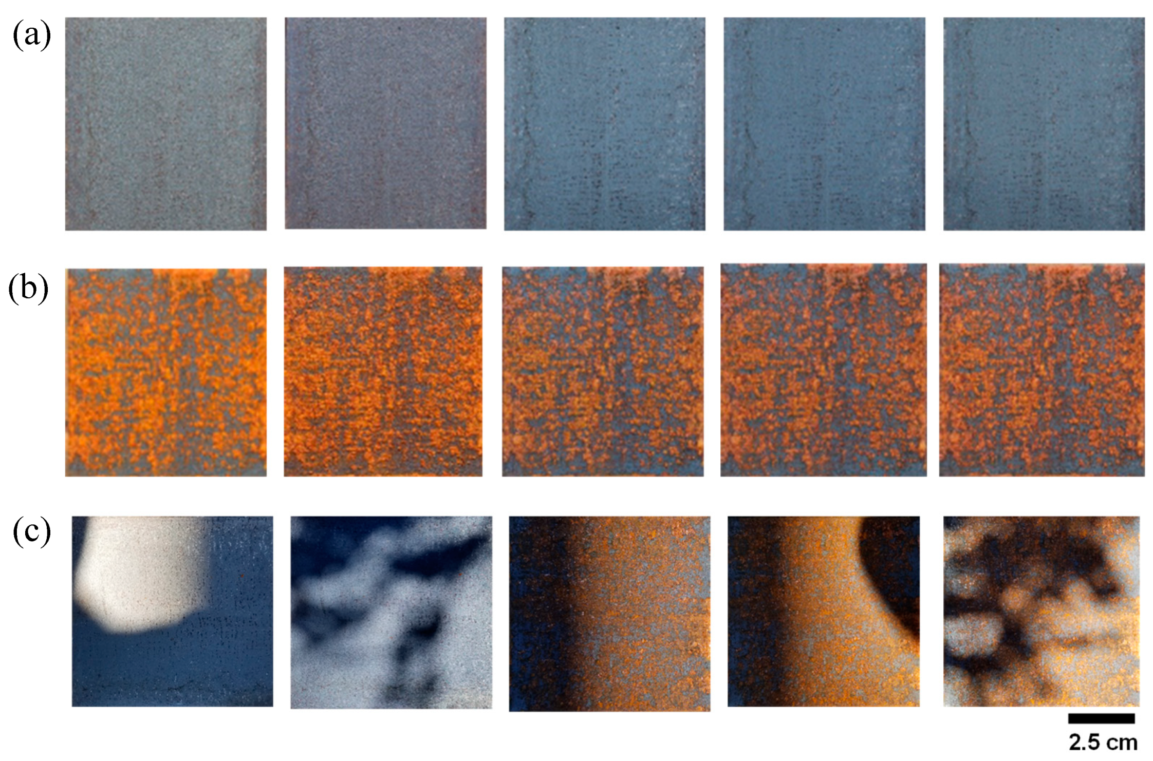
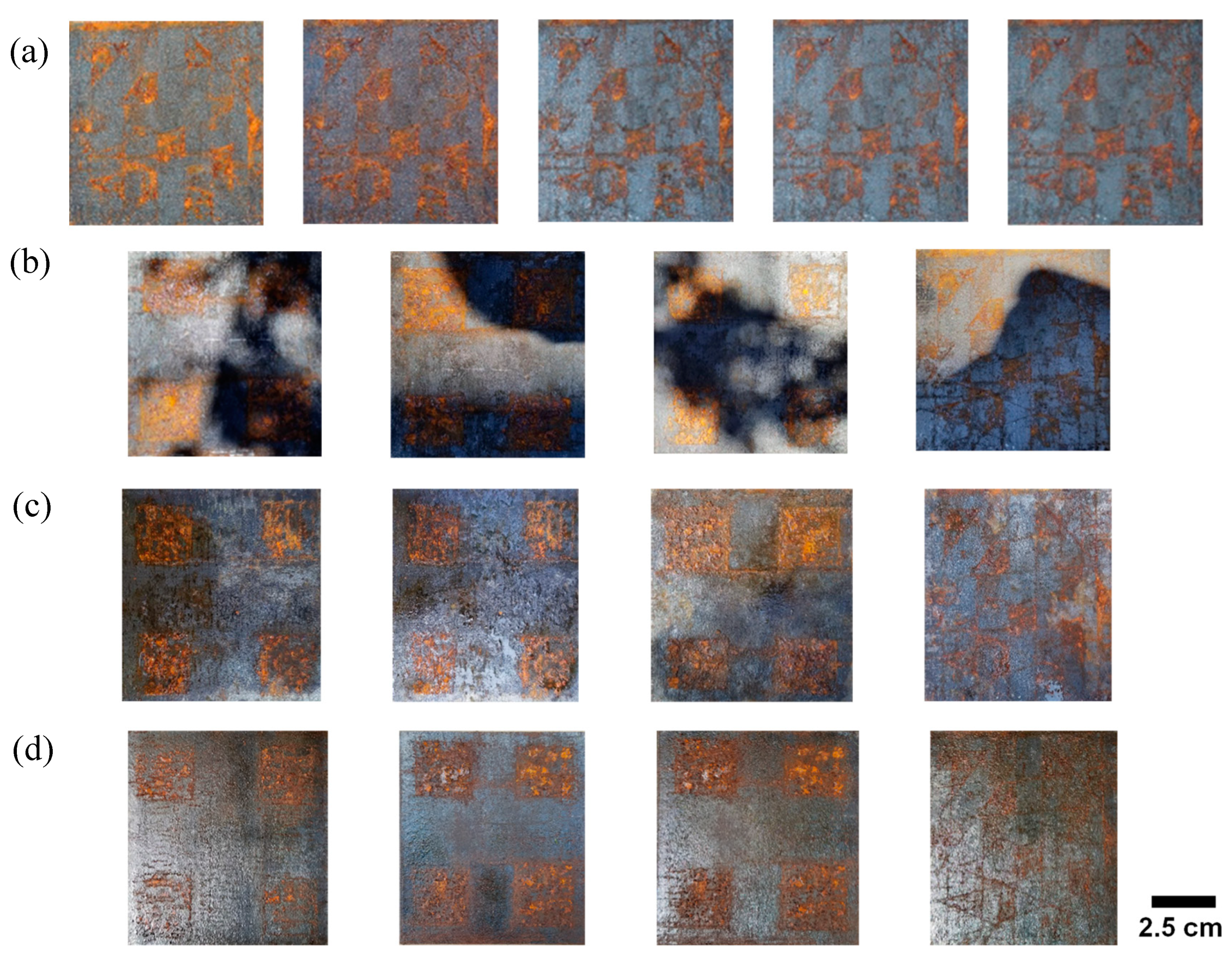
2. Laboratory Generated Corrosion Images

In this section, the procedure adopted for acquiring the lab generated corrosion images is described.

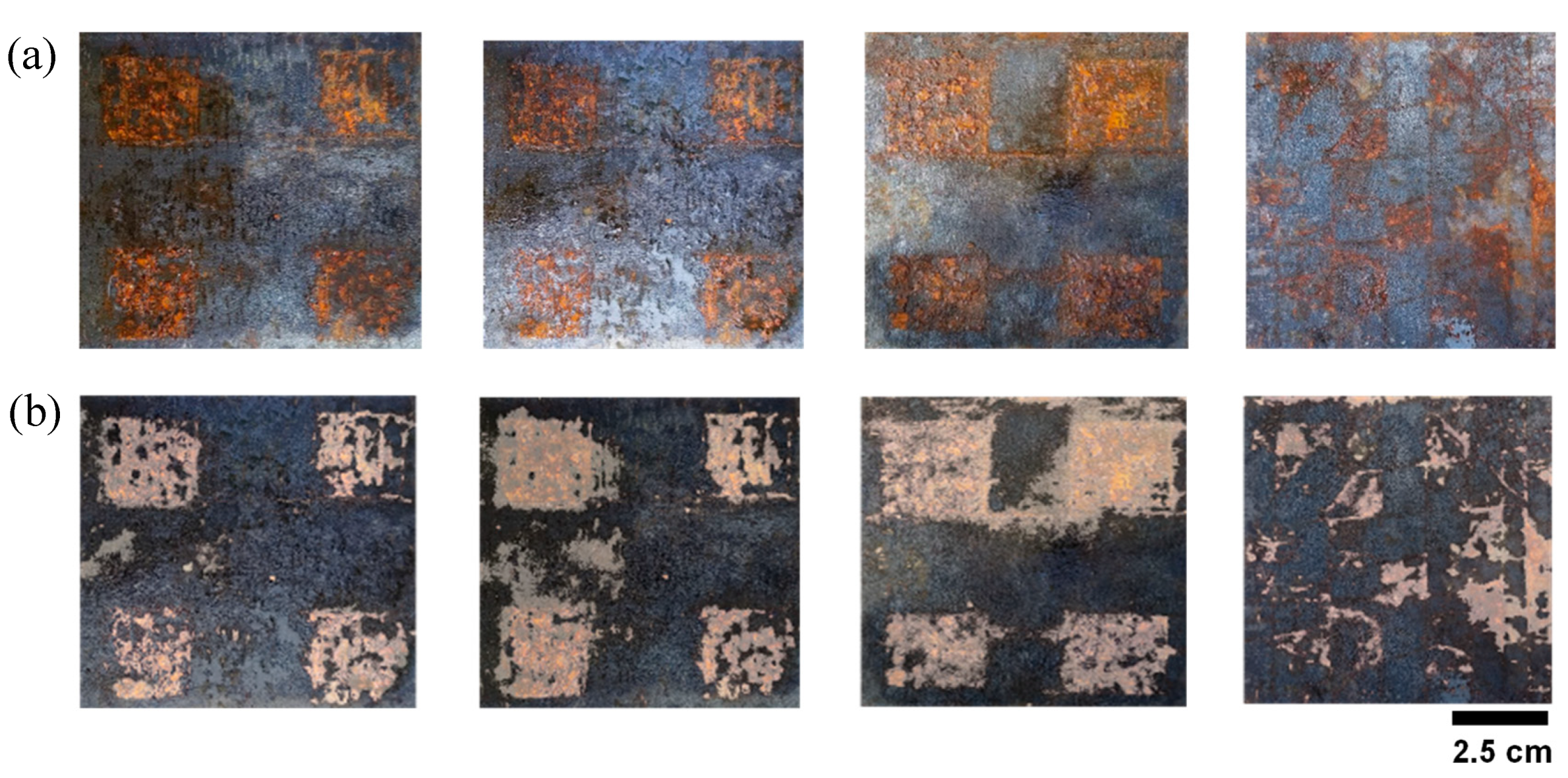
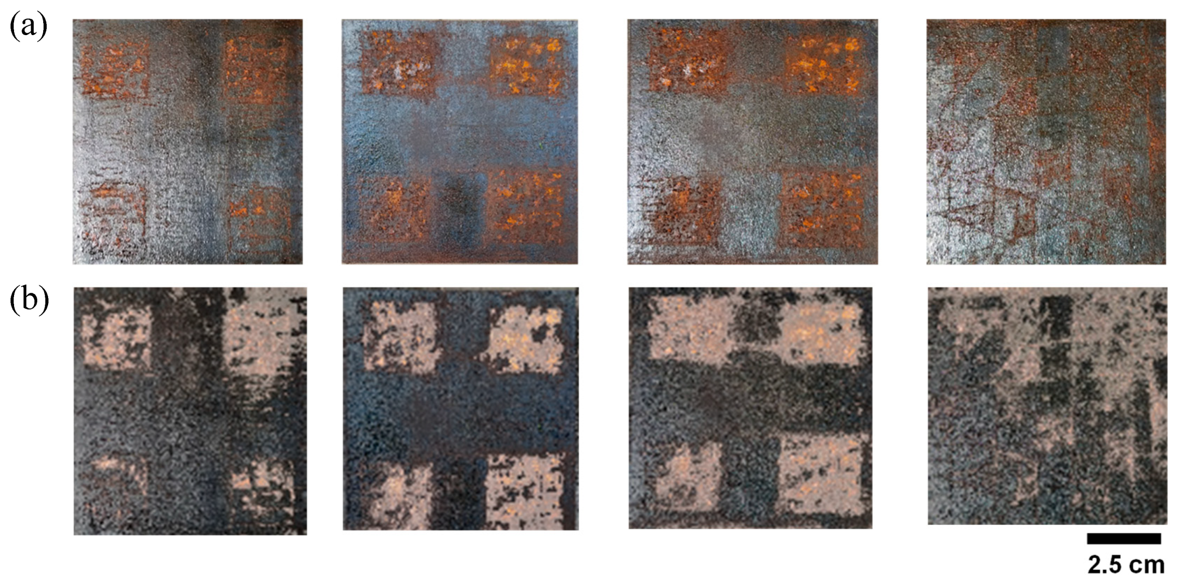
Accelerated Corrosion Tests and Image Acquisition

Six ASTM A36 structural steel plates (see

Table 1. ASTM A36 composition [29].

Composition	Symbol	wt. %
Carbon	C	0.25–0.29
Iron	Fe	98
Copper	Cu	0.2
Manganese	Mn	1.03
Phosphorous	P	0.04
Silicon	Si	0.28
Sulfur	S	0.05

[29]) with dimensions 7.6 cm $\times$ 7.6 cm $\times$ 0.4 cm are subjected to accelerated corrosion. To this end, ASTM A36 structural steel plates are placed inside a salt spray chamber at an angle of 20° to the vertical and are continuously exposed to 3.5 wt. % sodium chloride (NaCl) solution mist for 12 h. The corroded steel plates are then removed from the salt spray chamber and are gently cleaned with warm water to remove the excess salt traces and then air-dried. The detailed description of the accelerated corrosion protocol can be found elsewhere [30]. While the surfaces of two of the plates are completely exposed to corrosion (see Figure 1), the surfaces of rest of the plates are only partially exposed to corroded (see Figure 2) i.e., random patches of corrosion are induced on the plate by preventing the interaction between the corrosive media and the surface with the help of adhesive tapes. At this juncture, it is important to note that the plate surfaces completely exposed to corrosion are used for generating training and validation datasets and the plate surfaces partially exposed to corrosion are reserved for generating a test image database (see Section 3.4). Here on the plate surfaces completely exposed to corrosion will be referred to as fully corroded plates and the plate surfaces partially exposed to corrosion will be referred to as partially corroded plates. Details of generating training and test dataset are provided in Section 3.

A mobile camera (Samsung Electronics America Inc., Ridgefield Park, NJ, USA) with a digital resolution of 12 MP (4032 × 3024) is employed to acquire the images of the lab corroded steel plates. Note that the images were acquired outdoors while the corroded plates are directly exposed to sunlight. As per the manufacturer specifications, the size of the sensor and the size of the image pixel are 1/3.6" and 1.0 µm, respectively and the camera’s angular field of view (FOV) is 45°. For image acquisition, the camera is mounted on a small tripod and is placed parallel to the target surface (corroded plate) at a fixed distance of 8.0 inches. The camera was then operated with a fixed setting of ISO 400 and a shutter speed of 1/350th of a second. In addition to this, the color tone was set to a standard color tone and white balance was set to 5500 K (daylight). The images of the corroded steel plates are then acquired at different time intervals during the day i.e., 5:00 AM, 9:00 AM, 12:00 PM, 3:00 PM and 6:00 PM such that varying illuminations of daylight are captured in the images (see Figure 1a,b) Furthermore, the images of fully and partially corroded plates under shadows, water wetting, and oil wetting are also acquired. Shadows, water wetting, and oil wetting are commonly observed in steel structures such as bridges, water tanks, bunkers, and silos. Shadows are formed by blocking the light falling on the structure by surrounding vegetation, constructions, or the structural components that are being monitored. The water and oil wetting may occur due to rainfall and oil leak from cargo, respectively. The images of fully and partially corroded plates with shadows are acquired by blocking the light falling on the plate with an opaque object (see Figure 1c).

For acquiring the images of the fully and partially corroded plates wetted with water, the corroded steel plates are sprayed with the water using a spray jug obtained from a local store. Enough distance between corroded plates and spray jug is maintained such that only a drizzle of fine droplets of water is sprayed on the plate and sufficient care is exercised to avoid the formation of bigger water droplets on the surface of the plate. A similar procedure is then adopted for acquiring the images of fully and partially corroded plates under oil wetting except that oil is used in the place of water as a wetting agent. The images of all the corroded steel plates acquired using the mobile camera are shown in Figure 1 and Figure 2. Note that the images are not directly used as the input to the MLP in this study i.e., the images are not directly considered to be the training and validation datasets. Instead, color features of corroded and non-corroded pixels of the plate are extracted from the images to generate a training dataset and then used to train various MLP configurations. For instance, if the color features of 1000 corroded pixels are chosen from one image, then the training dataset is said to have 1000 observations. The color feature extraction process is described next.

3. Color Feature Extraction and Dataset Generation

In this study, we hypothesize that the color features alone can be used to identify corrosion in steel bridges. Hence color features are extracted from the lab-generated images to generate training, validation, and test datasets that will be used to train, validate, and demonstrate the performance of MLP, respectively. In this section, a brief overview of color spaces used in this study is provided and the process of generating training, validation, and test datasets is described.

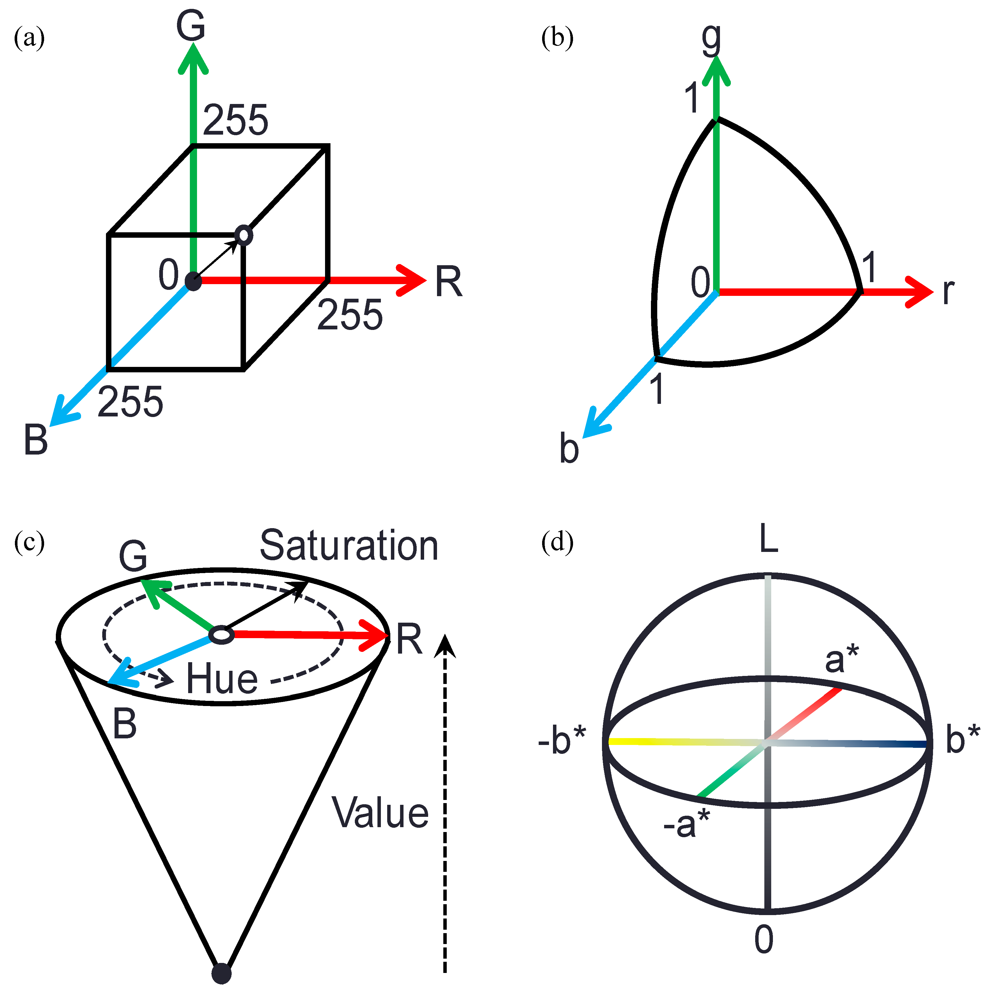
3.1. Color Spaces and Color Features

Color space is a mathematical abstraction introduced by Commission Internationale de l’éclairage (CIE) [31] to numerically express color as a tuple of numbers. It is regarded as the color coordinate system wherein each color feature is plotted along a coordinate axis. In this study, four-color spaces namely ‘RGB’ (also known as primary color space), ‘rgb’ (also known as normalized color space), ‘HSV’ (also known as perceptual color space) and ‘CIE La*b*’ (also known as uniform color space) are considered. A brief description of these four-color spaces is provided next.

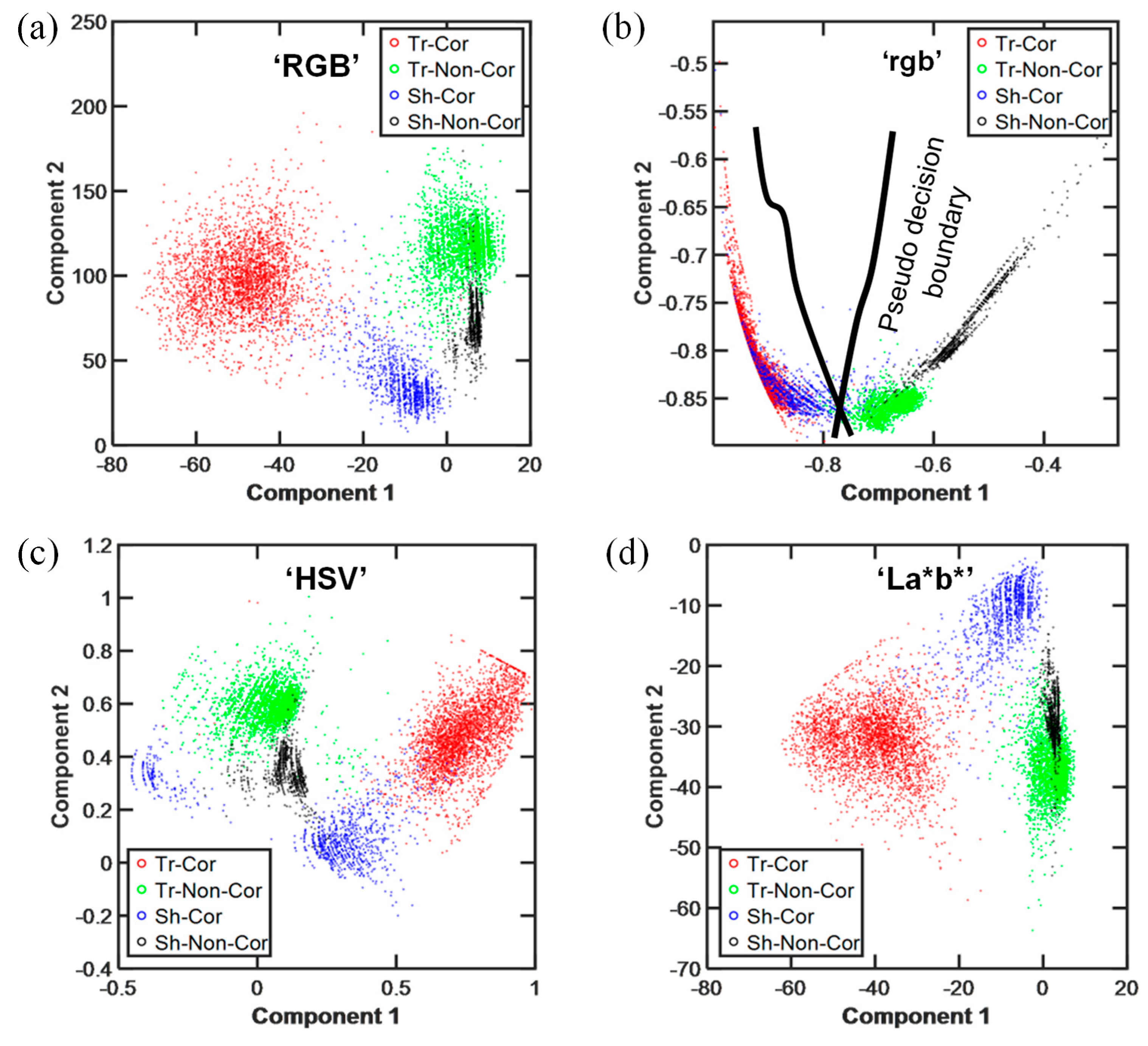
3.1.1. ‘RGB’ Color Space

In ‘RGB’ color space, the primary colors Red (R), Green (G) and Blue (B) are considered to be the color features whose intensities range from 0 to 255. These three-color intensities when plotted in a three-dimensional Cartesian coordinate system with primary colors $\left(\mathrm{R},\mathrm{G},\mathrm{B}\right)$ as the $x,y$ and $z$ axis, respectively, forms the ‘RGB’ color space. In the ‘RGB’ color space, all possible colors are encompassed in a cube with dimensions $\left(255 \times 255 \times 255\right)$ in the first positive octant of the coordinate system (see Figure 3a). Each point enclosed in this cube represents a unique color. While the point $\left(0,0,0\right)$ represents the black color, the point $\left(255, 255, 255\right)$ represents the white color. The points that fall on the line that joins origin $\left(0, 0, 0\right)$ and its diagonally opposite point $\left(255, 255, 255\right)$ represent different gray shades. Note that the color images obtained from the mobile or Digital Single-Lens Reflex (DSLR) cameras generally have intensities of R, G, and B as the pixel values. In the ‘RGB’ color space the chromaticity is coupled with the luminosity in the R, G, and B features and are sensitive to non-uniform illuminations.

3.1.2. ‘rgb’ Color Space

Unlike ‘RGB’ color space, in ‘rgb’ color space the normalized intensities of primary colors Red, Green and Blue are considered to be the color features. The magnitude of their intensities range from 0 to 1 and when plotted in a three-dimensional Cartesian coordinate system in which the normalized primary colors $\left(\mathrm{r},\mathrm{g},\mathrm{b}\right)$ are the $x,y$ and $z$ axis, respectively, each point represents a single unique color. In the ‘rgb’ color space, all possible colors are encompassed with-in the surface of a sphere in the first octant of the coordinate system where the radius of a sphere is 1 (see Figure 3b). To determine the values of ‘r’, ‘g’ and ‘b’, from ‘R’, ‘G’, and ‘B’ Equation (A1) (see Appendix A) is used. In ‘rgb’ color space the chromaticity and luminosity are decoupled from the r, g, and b features and, unlike ‘RGB’ color space the ‘rgb’ color space is insensitive to non-uniform illuminations [32].

3.1.3. ‘HSV’ Color Space

In ‘HSV’ color space, hue (H), Saturation (S) and Value (V) are considered to be the color features. Hue is defined as the pure color, and its magnitude ranges from 0 to 1. Saturation is defined as the amount of impurity or white color added to hue and its magnitude also ranges from 0 to 1. Value is defined as the brightness or intensity of light, and its magnitude ranges from 0 to 255. On a cylindrical coordinate system these color features i.e., Hue, Saturation and Value, represents the angle $(\mathsf{\theta }),$radius$\left(\mathrm{r}\right)$and vertical height $\left(\mathrm{z}\right)$, respectively. All the colors in the HSV color space fit in an inverted cone (see Figure 3c) [33]. Given, the intensities of R, G, and B, the magnitude of H, S, and V can be evaluated using Equations (A2)–(A5) (see Appendix A). Similar to ‘rgb’ color space, the chromaticity and luminosity are decoupled in the ‘HSV’ color space and is robust to non-uniform illuminations. However, in ‘HSV’ color space the chromaticity is represented as two separate features ‘Hue’ and ‘Saturation’. Moreover, ‘Hue’ is undefined when the intensities of R, G and, B are same.

3.1.4. ‘CIE La*b*’ Color Space

In ‘CIE La*b*’ color space, Lightness (L), and opponent colors (a* and b*) are considered to be the color features. While L represents the intensity of light and its magnitude ranges from 0 (white) to 100 (black), a* and b* represents the opponent colors red-green and blue-yellow respectively and its magnitude ranges from −128 to +128. The negative most value of a*, i.e., −128, represents the red color and positive most value of a*, i.e., 128, represents the green color. Similarly, the negative most value of b*, i.e., −128, represents the blue color and positive most value of b*, i.e., 128, represents the yellow color. These three-color features when plotted in a three-dimensional Cartesian coordinate system with $\left({\mathrm{a}}^{*},{\mathrm{b}}^{*},\mathrm{L}\right)$ as the $x,y$ and $z$ axis, respectively, forms the ‘La*b*’ color space. In the ‘CIE La*b*’ color space, all possible colors are encompassed in an ellipsoid (see Figure 3d) [34]. Each point enclosed in the ellipsoid represents a unique color. Given, the intensities of R, G, and B, the magnitude of L, a* and b*can be evaluated using Equation (A6) (see Appendix A). Similar to ‘rgb’ and ‘HSV’ color space, the chromaticity and luminosity are decoupled in ‘CIE La*b*’ color space and are insensitive to non-uniform illuminations. In addition to this, note that the ‘CIE La*b*’ color space is device independent and mimics the way humans perceive the colors [32].

3.2. Training Dataset

To obtain the training dataset the color features of corroded and non-corroded pixels are extracted from the lab generated images. Specifically, fully corroded steel plate images acquired under varying illuminations are considered for this purpose (see Section 2). For the extraction of color features the pixel information i.e., the intensity of primary colors R, G and B of the image is obtained in the MATLAB^® (MathWorks, Inc., Natick, MA, USA) and the Equations (A1)–(A6) provided in Appendix A is used to determine the color features in the other color spaces. A total of 5000 instances are generated for the training dataset among which 50% of the instances belonged to the ‘corrosion’ class and the rest of them belonged to the ‘non-corrosion’ class. Labelling of the instances as corrosion/non-corrosion is solely based on visual observation and judgement of the authors. As both ‘Non-corrosion’ and ‘Corrosion’ exhibit distinguishable color for trained human vision, the reproducibility of labeling can be assured. However, a slight chance for subjectivity cannot be ruled out. The overall goal of this body of research is to automate the optical corrosion detection by addressing the challenges associated with identifying corrosion under ambient lighting conditions. Hence, no corrosion characterization tests were performed to cross-validate the corrosion/non-corrosion pixels.

3.3. Validation Dataset

The validation dataset is used to validate a MLP that is trained using the color features extracted from lab acquired images of corroded plates under different illuminations (training dataset). The validation dataset is generated by extracting the color features of corroded and non-corroded pixels from the lab acquired images of corroded plates under shadows i.e., fully corroded steel plate images acquired under the shadow (see Figure 1c). Evaluation of the performance of the trained MLP on the validation dataset is seen as the first line of validation in this study and is used to identify an appropriate combination of MLP configuration and color features that can be ultimately used to detect corrosion in more challenging real-world scenarios. Note that none of the data instances in the validation dataset are used for training purposes. A total of 2064 instances are generated for the validation dataset, among which 50% of instances belong to ‘corrosion’ class and the rest of them belong to ‘non-corrosion’ class.

3.4. Test Image Database

The test image database will be used to test and demonstrate the efficacy of the trained and validated MLP to detect corrosion in digital images that have dark shadows and are acquired by a different imaging sensor. In other words, the generalization capability of the trained MLP to predict corrosion will be verified. The test image database generated herein includes the lab acquired images of partially corroded steel plates exposed to natural daylight illuminations (different from the ones used for training dataset), shadows and, water and oil wetting conditions and the images of a steel girder bridge located in Fargo-Moorhead (Minnesota) area acquired on-site. Note that the sensor employed for acquiring images in the laboratory and on-site bridge images are not the same. A Digital Single-Lens Reflex (DSLR) camera is used for acquiring the on-site bridge images. The DSLR camera has a resolution of 18 MP (5184 × 3456) with a pixel size of 4.3 µm and a 22.3 mm × 14.9 mm sensor size, and a sensor ratio of 3:2. The bridge images acquired on-site consist of the steel plate girders with naturally varying illumination and self-shadows. In particular, the images of the bottom side of the deck of the bridge had dark self-shadows. Note that in order to detect corrosion portions in the test images, the color features of each pixel in the test image have to be extracted first and then labeled by the trained MLP.

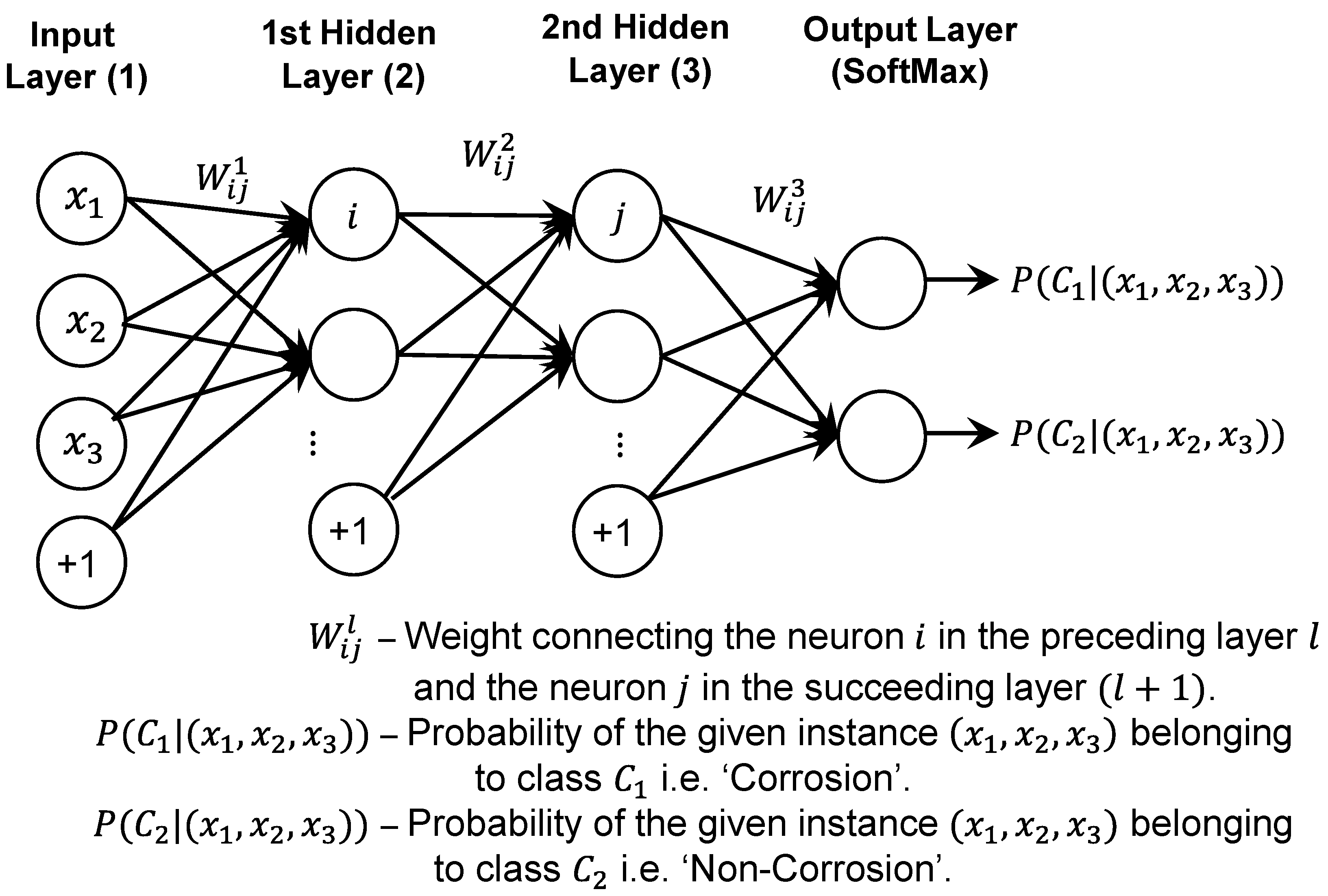
4. Multi-Layer Perceptron

A multi-layer feed-forward neural network, also referred to as multi-layer perceptron (MLP), is programmed in MATLAB^® (MathWorks, Inc., Natick, MA, USA) and is trained, validated, and tested in this study. The mathematical underpinnings and detailed description of multi-layer feed-forward neural network can be found elsewhere [35,36,37,38]. The MLP employed herein receives the color features of a pixel (see Section 3) as an input and delivers its class label (corrosion/non-corrosion) as an output (see Figure 4). Since the suitable configuration of MLP is not known apriori, four different configurations are explored: (1) one hidden layer (HL) with 2 neurons (1st HL(2N)), (2) one hidden layer with 4 neurons (1st HL(4N)), (3) two hidden layers with 2 neurons in each layer (1st HL(2N)-2nd HL(2N)) and (4) three hidden layers with 50 neurons in first layer, 10 neurons in second layer and 4 neurons in third layer (1st HL(50N)-2nd HL(10N)-3rd HL(4N)). Note that the selection of these configurations is based on thumb rules provided in the following references [39,40]. Sigmoid function is chosen as an activation function for all the neurons in the MLP except the output layer wherein SoftMax function is used and the maximum number of epochs is fixed to 1000. The maximum number of epochs is not exceeded in any case during the training phase. Furthermore, the MLP is trained only once (until the weights converged), and no re-training is required when used on in-house generated validation dataset or test image database. The back-propagation algorithm is used for determining the weights of the MLP.

5. Results

In this section, the best combination of the color space and an MLP configuration that can detect corrosion accurately under ambient lighting conditions is determined, and its efficacy in the real-world scenario is demonstrated. Test images described in Section 3.4 are employed for the purpose of demonstrating the efficacy i.e., the corroded portions in the lab generated images and steel bridge images are detected and provided.

5.1. Determining the Best Combination of Color Space and MLP

Sixteen combinations of MLP configurations and color spaces are assessed for determining the best combination i.e., the capability of each combination to predict the class labels (corrosion/ non-corrosion) accurately is evaluated. All the combinations are first trained with the training dataset (see Section 3.2) and then simultaneously deployed to predict the class labels in the validation dataset. The predicted class labels are cross-validated with the actual known class labels in the validation dataset and the summary of correct and incorrect classifications are provided in the form of a confusion matrix ($C$). The confusion matrix is a square matrix of size $m \times m$, where $m$ (=2) represents the number of class labels and the elements $C_{ij}$ represents the frequency of instances from the validation dataset that are assigned class label $j$ by the classifier which in reality they belong to class label $i$. Given the confusion matrix $C$, the performance of each combination is assessed by evaluating the four metrics namely ‘Accuracy’, ‘Precision’, ‘Recall’ and ‘F Measure’. ‘Accuracy’ is defined as the ratio of the total number of instances whose class labels are correctly identified to the total number of instances present in the validation dataset and is expressed as [20,41,42].

$$A=\frac{{\sum }_{i=1}^m{C}_{ii}}{{\sum }_{i=1}^m{\sum }_{j=1}^m{C}_{ij}}\times 100\%$$

(1)

‘Precision (O)’ is defined as the ratio of the number of observations whose class label $i$ is correctly predicted by the classifier to the total number of observations that are assigned to the class $i$ by the classifier, and ‘Recall (R)’ is defined as the proportion of observations of class $i$ that are correctly predicted as class $i$ by the classifier [41].

$$\mathrm{O}=\frac{1}{m}{\displaystyle \sum }_{i=1}^m\frac{C_{ii}}{{\sum }_{j=1}^m{C}_{ji}}\times 100\% \mathrm{R}=\frac{1}{m}{\displaystyle \sum }_{i=1}^m\frac{C_{ii}}{{\sum }_{j=1}^m{C}_{ij}}\times 100\%$$

(2)

Here, $m=2$ represents the number of class labels. While overall precision and overall recall are also used as the measures of performance assessment for classifiers, F-measure ($F$) combines the trade-off between both overall precision and overall recall and is evaluated as

$$\mathrm{F}=\frac{2\times O\times R}{O+R}\times 100\%$$

(3)

The confusion matrix and ‘Accuracy’ evaluated for each combination of MLP configuration and color space are summarized in

Table 2. Confusion matrix of the results predicted by various MLP configurations.

Color Space	Confusion Matrix
	2N		4N		2N-2N		50N-10N-4N
‘RGB’	0.33	0.67	0.35	0.65	0.36	0.64	0.61	0.39
	0	1	0	1	0	1	0	1
Acc.	66.50		67.50		68		80.50
‘rgb’	0.79	0.21	0.81	0.19	0.81	0.19	0.82	0.18
	0	1	0	1	0	1	0.03	0.97
Acc.	89.50		90.50		90.50		89.50
‘HSV’	0.66	0.34	0.68	0.32	0.70	0.30	0.60	0.40
	0.38	0.62	0.28	0.72	0	1	0.04	0.96
Acc.	64		70		85		78
‘La*b*’	0.39	0.61	0.51	0.49	0.54	0.46	0.31	0.69
	0	1	0	1	0	1	0	1
Acc.	69.50		75.50		77		65.50

Note: Acc.–Accuracy; Confusion matrix $\left[\begin{array}{cc}{c}_{11}& c_{12}\\ c_{21}& c_{22}\end{array}\right]$ where $c_{11 }and c_{22}$ represents the correct predictions corresponding to class labels corrosion and non-corrosion respectively, $c_{12 }and c_{21}$ represents the incorrect predictions corresponding to class labels corrosion and non-corrosion respectively.

. From Table 2, it can be inferred that the color spaces ‘RGB’ and ‘CIE La*b*’ resulted in a higher fraction of misclassification of ‘corrosion’ class label when compared to ‘rgb’ and ‘HSV’ color space i.e., on an average 65% of the instances in the training dataset belonging to ‘corrosion’ class are misclassified as ‘non-corrosion’ in the case of ‘RGB’ and ‘CIE La*b*’ color space (see also Figure 5). However, it is interesting to note that in the case of ‘RGB’ color space the accuracy improved when an additional hidden layer is added to the two-layer MLP configuration (see also Figure 5). The improvement in the accuracy of the ‘RGB’ color space may be attributed to the increased non-linearity or complexity in the decision boundary resulting from the addition of a hidden layer [43]. In other words, the decision boundary of a three-layer MLP maybe partitioning the training instances such that more fraction of the instances belonging to ‘corrosion’ class are on the same side of the boundary. Among the four-color spaces, the ‘rgb’ color space is found to yield a maximum prediction accuracy (91%). Despite the increase in the number of hidden layers the accuracy for the ‘rgb’ color space did not vary significantly (see Figure 5). To understand why the ‘rgb’ color space resulted in higher accuracy even without the addition of hidden layers, the color feature data is plotted as 2D scatter plots after dimensional reduction is performed on the training and validation datasets.

In the context of the current study, the dimensional reduction will facilitate visualizing a three-dimensional data (color features) in a two-dimensional space. Visualizing data in two-dimensional space will not only reveal the spatial distribution of instances belonging to ‘corrosion’ and ‘non-corrosion’ class but also aids in understanding the decision boundaries that can partition the instances with different class labels. Linear discriminant analysis (LDA) technique is used to perform dimensional reduction [44,45]. The results obtained after dimensional reduction for all four-color spaces are shown in Figure 6. Figure 6 consists of a scatterplot of four isolated groups that are labeled as ‘Tr_Corrosion’, ‘Tr_Non-corrosion’, ‘Sh_Corrosion’ and ‘Sh_Non-corrosion’. Note that the groups labeled as ‘Tr_Corrosion’ and ‘Tr_Non-corrosion’ correspond to the instances with class labels ‘corrosion’ and ‘non-corrosion’, respectively that are obtained from the training dataset and the groups ‘Sh_Corrosion’ and ‘Sh_Non-corrosion’ correspond to the instances with class labels ‘corrosion’ and ‘non-corrosion’, respectively obtained from the validation dataset. A trained MLP is anticipated to predict the class labels correctly when the instances of the ‘Tr_Corrosion’ and ‘Sh_Corrosion’ group remain on the same side of the decision boundary. In other words, the color features of the corroded pixels obtained from shaded regions (validation dataset) and varying illuminations (training dataset) should be on the same side of the decision boundary. In the case of ‘rgb’ color space, it may be true that the higher number of instances from ‘Tr_Corrosion’ and ‘Sh_Corrosion’ always remained on the same side of decision boundary irrespective of change in the shape of the boundary. For the sake of illustrating this point, the pseudo decision boundaries that may be resulting from two different MLP configurations are plotted in Figure 6b. From Figure 6b it can be understood that the instances partitioned by both the pseudo decision boundaries remains more or less similar.

Besides ‘Accuracy’, the other performance metrics ‘Precision’, ‘Recall’ and ‘F-measure’ are also evaluated and provided in

Table 3. Performance metrics of various MLP configurations.

Color Space		Performance Metrics (%)
		Accuracy	Recall	Precision	F-Measure
‘RGB’	2N	66.5	33	100	49.62
	4N	67.5	35	100	51.85
	2N-2N	68	36	100	52.94
	50N-10N-4N	80.5	61	100	75.78
‘rgb’	2N	89.5	79	100	88.27
	4N	90.5	81	100	89.50
	2N-2N	90.5	81	100	89.50
	50N-10N-4N	89.5	81	100	90.11
‘HSV’	2N	64	66	63	64.47
	4N	70	68	70	68.99
	2N-2N	85	70	100	82.35
	50N-10N-4N	78	60	100	75.00
‘La*b*’	2N	69.5	39	100	56.12
	4N	75.5	51	100	67.55
	2N-2N	77	54	100	70.13
	50N-10N-4N	65.5	31	100	47.33

. For most of the combinations of MLP and color spaces the ‘Precision’ value is 100%. This can be attributed to the zero false positive value of the ‘Corrosion’ class label i.e., no ‘Non-corrosion’ class labels are incorrectly predicted as ‘Corrosion’. However, the ‘Recall’ and ‘F-measure’ value varied for different combinations. Note that the ‘Recall’ with a higher magnitude is preferred instead of ‘Accuracy’ for choosing the best combination of MLP and color space. ‘Recall’ measures the ability of a model to predict the actual ‘Corrosion’ class label as ‘Corrosion’ which is highly desired. Based on the assessment of ‘Recall’ values for all the combinations i.e., a single hidden layer with 4 neurons (1st HL (4N)) MLP configuration with ‘rgb’ color space is chosen as the best combination in this study.

5.2. Detection of Corrosion in Lab Generated Test Images

An MLP configuration consisting of single hidden layer with 4 neurons (1st HL (4N)) trained on ‘rgb’ color features and is deployed to detect corroded portions in the lab generated test images and the results obtained are shown in Figure 7, Figure 8, Figure 9 and Figure 10. Note the corroded portions are represented as a bright mask in the Figure 7b, Figure 8b, Figure 9b and Figure 10b. For qualitative comparison, the ground truth images are also provided along with the corrosion detected images (see Figure 7a, Figure 8a, Figure 9a and Figure 10a). While Figure 7 and Figure 8 consists of test images acquired under varying illuminations and cast shadows, respectively, Figure 9 and Figure 10 consists of test images acquired under water and oil wetting, respectively. From Figure 7, Figure 8, Figure 9 and Figure 10, it is evident that the trained MLP detects corrosion accurately in the test images that are acquired under varying illuminations, shadows, water wetting, and oil wetting conditions. Despite the presence of light shadows and dark shadows found in Figure 8 and the wetting conditions found in Figure 9 and Figure 10, the single hidden with 4 neurons (4N) MLP trained with ‘rgb’ color features predicted corrosion accurately. However, in the case of water and oil wetted test images some specular reflections are observed, and it is highly unlikely to detect corrosion under such a scenario. Specular reflections are the mirror-like reflections commonly observed on smooth surfaces of bodies where the angle of incidence of light is equal to the angle of reflection [46].

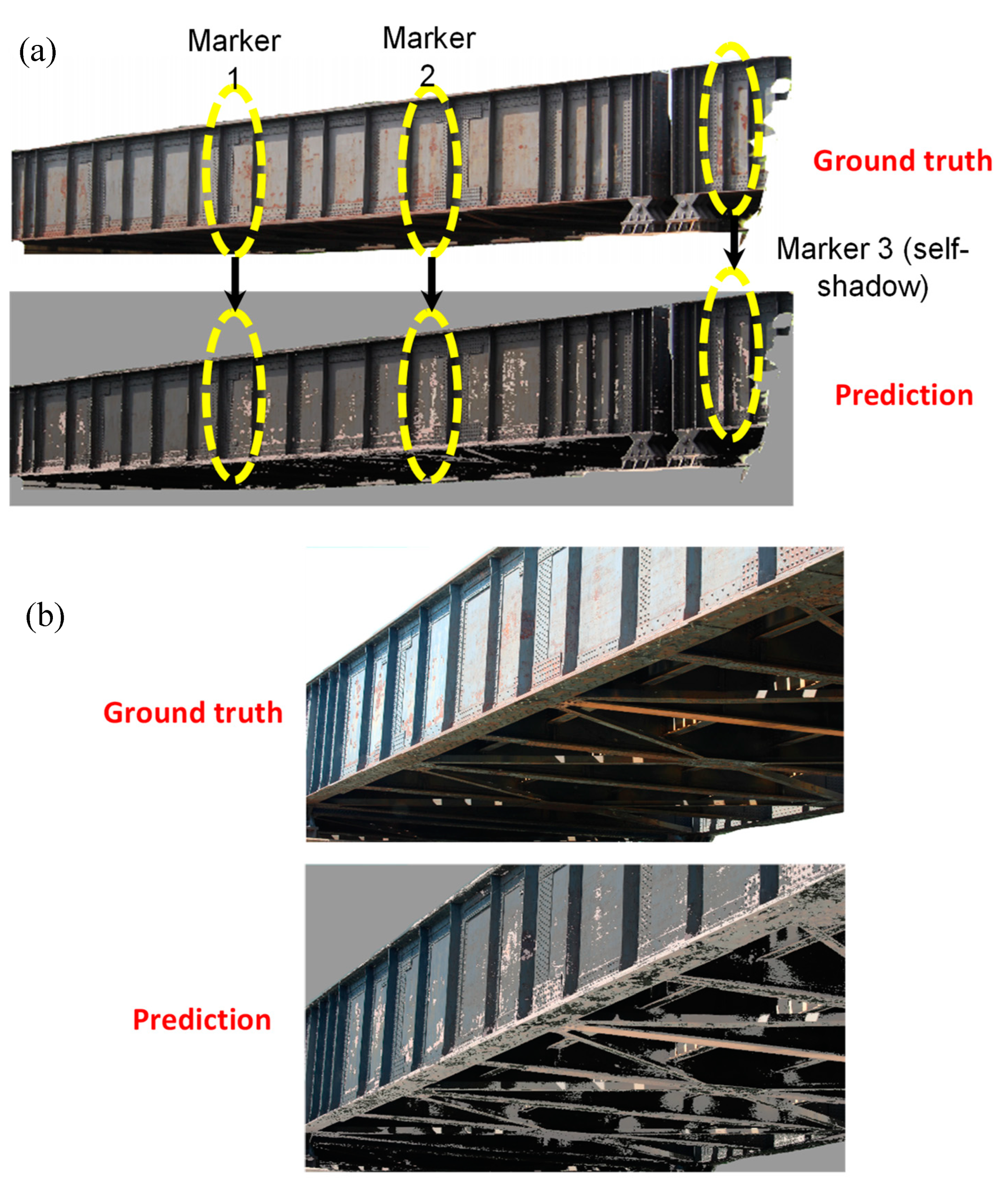
5.3. Detection of Corrosion in Steel Bridge

An MLP configuration consisting of single hidden layer with 4 neurons (1st HL (4N)) trained on ‘rgb’ color features is finally deployed to detect corroded portions in the steel bridge images and the results obtained are shown in Figure 11. Similar to Figure 7, Figure 8, Figure 9 and Figure 10, the corroded portions of the bridge are highlighted as a bright mask in Figure 11 and the ground truth images are provided for a qualitative comparison. From Figure 11, it can be observed that the trained MLP detects corrosion accurately in the steel girder bridges under naturally varying illuminations and self-shadows. While ‘Marker 1′ and ‘Marker 2′ shown in Figure 11a reveals the ability of the trained MLP to detect corrosion under brighter illumination, ‘Marker 3′ indicates the ability of the trained MLP to detect corrosion under comparatively darker illuminations and self-shadows. Further from Figure 11b it is also evident that the trained MLP configuration of single hidden layer with 4 neurons (1st HL (4N)) is able to predict corrosion in the bottom side of the deck of the bridge that has a dark shadow. At this juncture, it is important to emphasize the fact that it is highly unlikely for a human vision to detect corrosion under dark shadows. Keeping in view that a greater portion of corrosion is found in the bottom side of the deck of the bridge, the proposed method will be very useful.

6. Conclusions and Limitations

Color spaces in conjunction with different MLP configurations are explored to detect corrosion initiation in steel structures under ambient lighting conditions. To this end, 16 different combinations of color spaces and MLP configurations are explored. The performance of each combination is then assessed through the validation dataset obtained from lab generated images and the best combination is determined. Subsequently, the obtained combination is deployed on the test image database and the efficacy of trained MLP to detect corrosion in real-world scenarios is demonstrated.

From the current study following conclusions can be drawn.

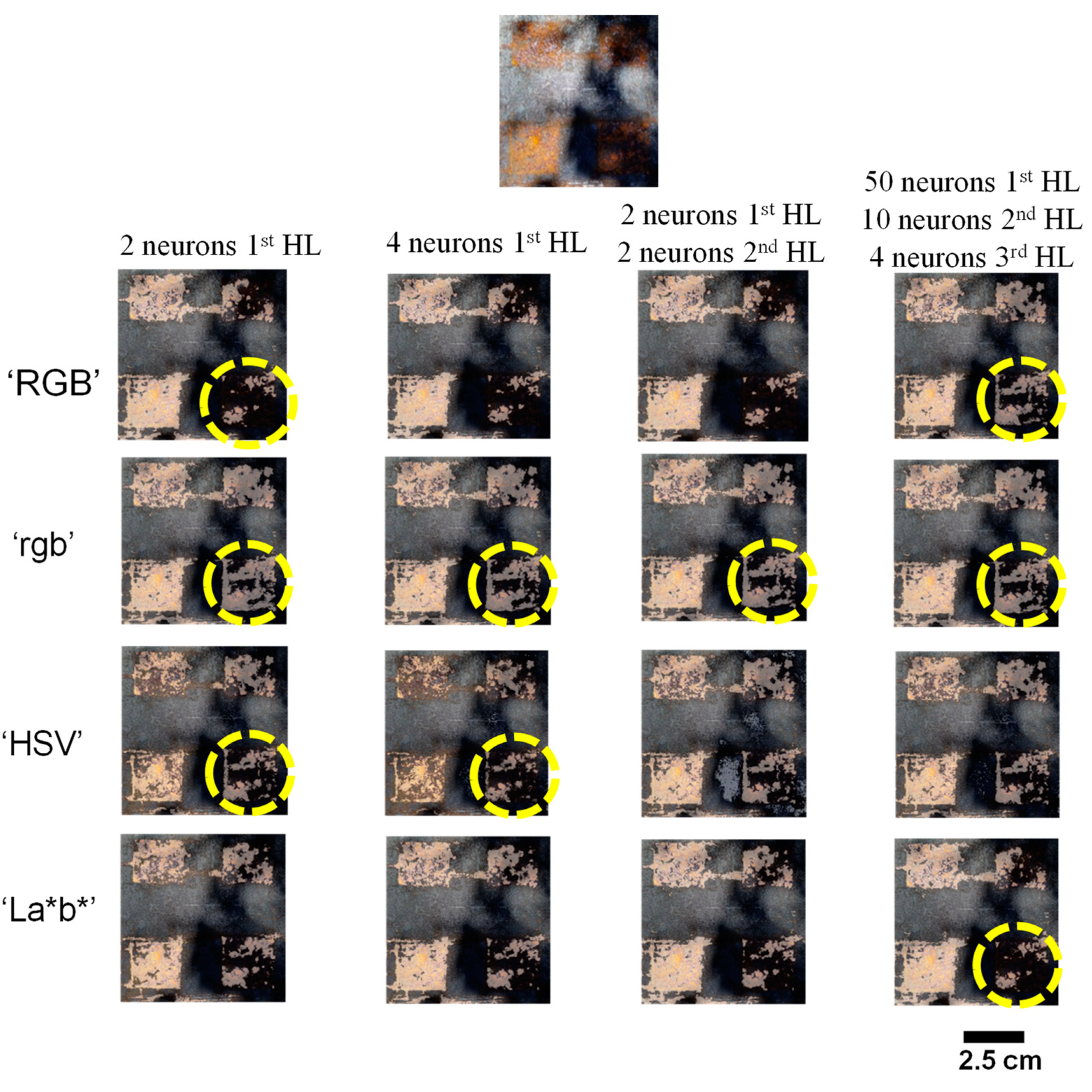
• Among all 16 combinations of color space and an MLP configuration, the combination of ‘rgb’ color space and an MLP configuration of a single hidden layer with 4 neurons (1st HL (4N)) yielded the highest ‘Recall’ of 81% and hence chosen as the best combination.
• While the accuracy (up to 91%) of ‘rgb’ color space is found to be more or less similar for all the MLP configurations, the accuracy of ‘RGB’ color space is observed to increase from 68% to 81% with the addition of third hidden layer. Improved accuracy in the case of ‘RGB’ color space can be attributed to the increased non-linearity of the decision boundary generated by the MLP which will ultimately lead to overfitting issues.
• Under shadows and wetting conditions, the trained MLP is still found to yield correct predictions when ‘rgb’ color features are used. In particular, the detection of corrosion in the bottom side of the deck of a bridge under dark shadows is noteworthy.
• The proposed method is insensitive to the camera sensor employed for the image acquisition i.e., irrespective of images being acquired from a mobile camera or a DSLR camera the efficacy of trained MLP to detect corrosion was not affected.
• MLP trained on varying illumination dataset alone is sufficient for detecting the corrosion under shadows and wetting conditions.

Although the efficacy of color spaces for corrosion detection is demonstrated in this study, it is important to note that the employment of color features alone may have some limitations. One case where this technique is not applicable is when the objects in the acquired images possess hue values similar to that of a corroded surface. For instance, coatings, dirt, or some vegetation in the background may be misclassified as corrosion. This limitation will be addressed in future work by the authors.

References

1. Troitsky, M.S. Planning and Design of Bridges; John Wiley & Sons, Inc.: New York, NY, USA, 1994. [Google Scholar]
2. Haas, T. Are Reinforced Concrete Girder Bridges More Economical Than Structural Steel Girder Bridges? A South African Perspective. Jordan J. Civ. Eng. 2014, 159, 1–15. [Google Scholar] [CrossRef]
3. Sastri, V.S. Challenges in Corrosion: Costs, Causes, Consequences, and Control; John Wiley & Sons: Hoboken, NJ, USA, 2015. [Google Scholar]
4. Chen, W.-F.; Duan, L. Bridge Engineering Handbook: Construction and Maintenance; CRC Press: Boca Raton, FL, USA, 2014. [Google Scholar]
5. García-Martín, J.; Gómez-Gil, J.; Vázquez-Sánchez, E. Non-Destructive Techniques Based on Eddy Current Testing. Sensors 2011, 11, 2525–2565. [Google Scholar] [CrossRef] [PubMed] [Green Version]
6. Pavlopoulou, S.; Staszewski, W.; Soutis, C. Evaluation of instantaneous characteristics of guided ultrasonic waves for structural quality and health monitoring. Struct. Control Health Monit. 2012, 20, 937–955. [Google Scholar] [CrossRef]
7. Sharma, S.; Mukherjee, A. Ultrasonic guided waves for monitoring corrosion in submerged plates. Struct. Control Health Monit. 2015, 22, 19–35. [Google Scholar] [CrossRef]
8. Nowak, M.; Lyasota, I.; Baran, I. The test of railway steel bridge with defects using acoustic emission method. J. Acoust. Emiss. 2016, 33, 363–372. [Google Scholar]
9. Cole, P.; Watson, J. Acoustic emission for corrosion detection. In Advanced Materials Research; Trans Tech Publications Ltd.: Stafa-Zurich, Switzerland, 2006; pp. 231–236. [Google Scholar]
10. Deraemaeker, A.; Reynders, E.; De Roeck, G.; Kullaa, J. Vibration-based structural health monitoring using output-only measurements under changing environment. Mech. Syst. Signal Process. 2008, 22, 34–56. [Google Scholar] [CrossRef] [Green Version]
11. McCrea, A.; Chamberlain, D.; Navon, R. Automated inspection and restoration of steel bridges—A critical review of methods and enabling technologies. Autom. Constr. 2002, 11, 351–373. [Google Scholar] [CrossRef]
12. Doshvarpassand, S.; Wu, C.; Wang, X. An overview of corrosion defect characterization using active infrared thermography. Infrared Phys. Technol. 2019, 96, 366–389. [Google Scholar] [CrossRef]
13. Jahanshahi, M.R.; Kelly, J.S.; Masri, S.F.; Sukhatme, G.S. A survey and evaluation of promising approaches for automatic image-based defect detection of bridge structures. Struct. Infrastruct. Eng. 2009, 5, 455–486. [Google Scholar] [CrossRef]
14. Chen, P.-H.; Chang, L.-M. Artificial intelligence application to bridge painting assessment. Autom. Constr. 2003, 12, 431–445. [Google Scholar] [CrossRef]
15. Chen, P.-H.; Yang, Y.-C.; Chang, L.-M. Automated bridge coating defect recognition using adaptive ellipse approach. Autom. Constr. 2009, 18, 632–643. [Google Scholar] [CrossRef]
16. Shen, H.-K.; Chen, P.-H.; Chang, L.-M. Automated steel bridge coating rust defect recognition method based on color and texture feature. Autom. Constr. 2013, 31, 338–356. [Google Scholar] [CrossRef]
17. Gevers, T.; Gijsenij, A.; Van De Weijer, J.; Geusebroek, J.-M. Color in Computer Vision: Fundamentals and Applications; John Wiley & Sons: Hoboken, NJ, USA, 2012. [Google Scholar]
18. Koschan, A.; Abidi, M. Digital Color Image Processing; John Wiley & Sons: Hoboken, NJ, USA, 2008. [Google Scholar]
19. Zhang, Z.; Flores, P.; Igathinathane, C.; Naik, D.L.; Kiran, R.; Ransom, J.K. Wheat Lodging Detection from UAS Imagery Using Machine Learning Algorithms. Remote Sens. 2020, 12, 1838. [Google Scholar] [CrossRef]
20. Naik, D.L.; Kiran, R. Identification and characterization of fracture in metals using machine learning based texture recognition algorithms. Eng. Fract. Mech. 2019, 219, 106618. [Google Scholar] [CrossRef]
21. Medeiros, F.N.; Ramalho, G.L.B.; Bento, M.P. On the Evaluation of Texture and Color Features for Nondestructive Corrosion Detection. Eurasip J. Adv. Signal Process. 2010, 2010, 817473. [Google Scholar] [CrossRef] [Green Version]
22. Ranjan, R.; Gulati, T. Condition assessment of metallic objects using edge detection. Int. J. Adv. Res. Comput. Sci. Softw. Eng. 2014, 4, 253–258. [Google Scholar]
23. Lee, S.; Chang, L.-M.; Skibniewski, M. Automated recognition of surface defects using digital color image processing. Autom. Constr. 2006, 15, 540–549. [Google Scholar] [CrossRef]
24. Chen, P.-H.; Shen, H.-K.; Lei, C.-Y.; Chang, L.-M. Support-vector-machine-based method for automated steel bridge rust assessment. Autom. Constr. 2012, 23, 9–19. [Google Scholar] [CrossRef]
25. Ghanta, S.; Karp, T.; Lee, S. Wavelet domain detection of rust in steel bridge images. In Proceedings of the 2011 IEEE International Conference on Acoustics, Speech and Signal Processing (ICASSP), Prague, Czech Republic, 22–27 May 2011. [Google Scholar]
26. Nelson, B.N.; Slebodnick, P.; Lemieux, E.J.; Singleton, W.; Krupa, M.; Lucas, K.; Ii, E.D.T.; Seelinger, A. Wavelet processing for image denoising and edge detection in automatic corrosion detection algorithms used in shipboard ballast tank video inspection systems. In Proceedings of the Wavelet Applications VIII: International Society for Optics and Photonics, Orlando, FL, USA, 26 March 2001. [Google Scholar]
27. Son, H.; Hwang, N.; Kim, C.; Kim, C. Rapid and automated determination of rusted surface areas of a steel bridge for robotic maintenance systems. Autom. Constr. 2014, 42, 13–24. [Google Scholar] [CrossRef]
28. Liao, K.-W.; Lee, Y.-T. Detection of rust defects on steel bridge coatings via digital image recognition. Autom. Constr. 2016, 71, 294–306. [Google Scholar] [CrossRef]
29. Sajid, H.U.; Naik, D.L.; Kiran, R. Microstructure–Mechanical Property Relationships for Post-Fire Structural Steels. J. Mater. Civ. Eng. 2020, 32, 04020133. [Google Scholar] [CrossRef]
30. Sajid, H.U.; Kiran, R. Influence of corrosion and surface roughness on wettability of ASTM A36 steels. J. Constr. Steel Res. 2018, 144, 310–326. [Google Scholar] [CrossRef]
31. Delgado-González, M.J.; Carmona-Jiménez, Y.; Rodríguez-Dodero, M.C.; García-Moreno, M.V. Color Space Mathematical Modeling Using Microsoft Excel. J. Chem. Educ. 2018, 95, 1885–1889. [Google Scholar] [CrossRef]
32. Garcia-Lamont, F.; Cervantes, J.; López, A.; Rodriguez, L. Segmentation of images by color features: A survey. Neurocomputing 2018, 292, 1–27. [Google Scholar] [CrossRef]
33. Smith, A.R. Color gamut transform pairs. ACM Siggraph Comput. Graph. 1978, 12, 12–19. [Google Scholar] [CrossRef]
34. Liu, G.-H.; Yang, J.-Y. Exploiting Color Volume and Color Difference for Salient Region Detection. IEEE Trans. Image Process. 2018, 28, 6–16. [Google Scholar] [CrossRef]
35. Shanmuganathan, S. Artificial Neural Network Modelling: An Introduction. In Intelligent Distributed Computing VI; Springer Science and Business Media LLC: Cham, Switzerland, 2016; pp. 1–14. [Google Scholar]
36. Priddy, K.L.; Keller, P.E. Artificial Neural Networks: An Introduction; SPIE Press: Bellingham, WA, USA, 2005. [Google Scholar]
37. Aggarwal, C.C. Neural Networks and Deep Learning; Springer International Publishing: Cham, Switzerland, 2018. [Google Scholar]
38. Daniel, G. Principles of Artificial Neural Networks; World Scientific: Hoboken, NJ, USA, 2013. [Google Scholar]
39. Leva, S.; Ogliari, E. Computational Intelligence in Photovoltaic Systems. Appl. Sci. 2019, 9, 1826. [Google Scholar] [CrossRef] [Green Version]
40. Engel, T.; Gasteiger, J. Chemoinformatics: Basic Concepts and Methods; Wiley-VCH: Weinheim, Germany, 2018. [Google Scholar]
41. Naik, D.L.; Sajid, H.U.; Kiran, R. Texture-Based Metallurgical Phase Identification in Structural Steels: A Supervised Machine Learning Approach. Metals 2019, 9, 546. [Google Scholar] [CrossRef] [Green Version]
42. Naik, D.L.; Kiran, R. Naïve Bayes classifier, multivariate linear regression and experimental testing for classification and characterization of wheat straw based on mechanical properties. Ind. Crop. Prod. 2018, 112, 434–448. [Google Scholar] [CrossRef]
43. Sethi, I.K.; Jain, A.K. Artificial Neural Networks and Statistical Pattern Recognition: Old and New Connections; Elsevier: Amsterdam, The Netherlands, 2014. [Google Scholar]
44. Li, C.; Wang, B. Fisher Linear Discriminant Analysis. Available online: https://www.ccs.neu.edu/home/vip/teach/MLcourse/5_features_dimensions/lecture_notes/LDA/LDA.pdf (accessed on 27 October 2020).
45. Gu, Q.; Li, Z.; Han, J. Linear discriminant dimensionality reduction. In Joint European Conference on Machine Learning and Knowledge Discovery in Databases; Springer: Berlin/Heidelberg, Germany, 2011; pp. 549–564. [Google Scholar]
46. Tan, K.; Cheng, X. Specular Reflection Effects Elimination in Terrestrial Laser Scanning Intensity Data Using Phong Model. Remote. Sens. 2017, 9, 853. [Google Scholar] [CrossRef] [Green Version]
47. Lee, H.-C. Introduction to Color Imaging Science; Cambridge University Press: Cambridge, UK, 2005. [Google Scholar]
48. Mestha, L.K.; Dianat, S.A. Control of Color Imaging Systems: Analysis and Design; CRC Press: Boca Raton, FL, USA, 2009. [Google Scholar]
Figure 1. Non-corroded and corroded steel plates used for training purposes. (a) top row (left to right) includes images of non-corroded plates acquired at varying illuminations under natural daylight, (b) second row (left to right) includes images of corroded plates acquired under illuminations similar to that of non-corroded plates and, (c) third row (left to right) includes images of both corroded and non-corroded plates acquired under casted shadows.
Metals 10 01439 g001
Figure 2. Images of partially corroded steel plates used for testing: (a) acquired at different illuminations of natural daylight, (b) shadows, (c) water wetting, and (d) oil wetting.
Metals 10 01439 g002
Figure 3. Color spaces in three-dimensional coordinate systems: (a) ‘RGB’, (b) ‘rgb’, (c) ‘HSV’ and (d) ‘CIE La*b*’.
Metals 10 01439 g003
Figure 4. Schematic of a multi-layer perceptron configuration for the classification of the labeled data. Note that the input features x 1 , x 2 and x 3 represent three color features associated with ‘RGB’, ‘rgb’, ‘HSV’ and ‘La*b*’ color spaces respectively.
Metals 10 01439 g004
Figure 5. Prediction of corrosion in a test image (with shadow) using four different color spaces and four different ANN configurations. Markers for ‘RGB’–accuracy improved for three-layer MLP; Markers for ‘rgb’–accuracy remained almost same; Markers for ‘HSV’–accuracy is poor for 2 and 4 neurons MLP configuration; Markers for ‘CIE La*b*’–accuracy is poor for three-layer MLP configuration. Note HL–hidden layer.
Metals 10 01439 g005
Figure 6. Dimensional reduction using LDA. Training dataset encompassing 4 class labels namely corrosion (Tr-Cor), non-corrosion (Tr-Non-Cor), corrosion in shadow (Sh-Cor) and non-corrosion (Sh-Non-Cor) in shadow are visualized in a 2-dimensional space. (a) RGB, (b) rgb, (c) HSV and (d) La*b*.
Metals 10 01439 g006
Figure 7. Test images of partially corroded steel plates acquired at different illuminations of natural daylight. (a) ground truth images, (b) MLP-based corrosion prediction.
Metals 10 01439 g007
Figure 8. Test images of partially corroded steel plates with shadows cast in natural daylight. (a) ground truth images, (b) MLP-based corrosion prediction.
Metals 10 01439 g008
Figure 9. Test images of partially corroded steel plates wetted in water and acquired in natural daylight. (a) ground truth images, (b) MLP-based corrosion prediction.
Metals 10 01439 g009
Figure 10. Test images of partially corroded steel plates wetted in oil and acquired in natural daylight. (a) ground truth images, (b) MLP-based corrosion prediction.
Metals 10 01439 g010
Figure 11. Identification of corrosion in the steel bridges using the single hidden layer with 4 neurons (1st HL(4N)) MLP Configuration. (a) steel plate girders with naturally varying illumination and self-shadows, (b) bottom side of the deck of the bridge with dark self-shadows.
Metals 10 01439 g011