
A New Material Model for Agglomerated Cork
by
 , and
, and
Gabriel Thomaz de Aquino Pereira
1,
Ricardo J. Alves de Sousa
2,3 ,
,
I-Shih Liu
4,
Marcello Goulart Teixeira
1,* and
Fábio A. O. Fernandes
2,3
1
Intitute of Computing, Federal University of Rio de Janeiro, Rio de Janeiro 21941-853, Brazil
2
TEMA—Centre for Mechanical Technology and Automation, Department of Mechanical Engineering, University of Aveiro, 3810-193 Aveiro, Portugal
3
LASI—Intelligent Systems Associate Laboratory, 4800-058 Guimarães, Portugal
4
Intitute of Mathematics, Federal University of Rio de Janeiro, Rio de Janeiro 21941-853, Brazil
*
Author to whom correspondence should be addressed.
Math. Comput. Appl. 2022, 27(6), 92; https://doi.org/10.3390/mca27060092
Submission received: 3 September 2022
/
Revised: 5 November 2022
/
Accepted: 7 November 2022
/
Published: 9 November 2022
(This article belongs to the Collection Feature Papers in Mathematical and Computational Applications)
Abstract
:It is increasingly necessary to promote means of production that are less polluting and less harmful to the environment following the UN 2030 agenda for sustainable development. Using natural cellular materials in structural applications can be essential for enabling a future in this direction. Cork is a natural cellular material with an excellent energy absorption capacity. Its use in engineering applications and products has grown over time, so predicting its mechanical response through numerical tools is crucial. Classical cork modeling uses a model developed for foam material, including an adjustment function that does not have a clear physical interpretation. This work presents a new material model for an agglomerated cork based solely on well-known hypotheses of continuum mechanics using fewer parameters than the classical model and further a finite element framework to validate the new model against experimental data.
1. Introduction
The use of cellular materials in engineering applications has been established worldwide. This kind of material has excellent crashworthiness and insulation properties. Styrofoam (expanded polystyrene), derived from oil, is widely present in packaging and safety apparel, with excellent cost/performance ratios but with well-known recyclability and biodegradability issues after usage. Cork, the outer bark of Quercus suber L. tree, is a natural cellular material by excellence, allying crashworthiness and insulation properties. Compared with its synthetic counterparts, it is a sustainable and eco-friendly solution.
Dart and Eugene [1] made one of the first attempts to characterize cork mechanical behavior under compression loading. They found that each stress–time curve for various compressions can be obtained from each other by scaling. Such scalability was justified by the shape of the stress–strain compression curve. A highly non-linear stress–strain response curve characterizes agglomerated cork under compression. This curve is divided into three parts: a small elastic linear behavior at the beginning, followed by a plateau, and finished with a highly non-linear densification part.
All types of cork, natural, agglomerated, and expanded, are characterized by this compression behavior. The material properties vary with density, cellular dimensions, and porosity, as seen in [2,3]. The Poisson effect in natural cork compression was studied by [4]. They found that for compression in axial and tangential directions, the Poisson’s ratio is almost null, while in the radial direction, cork presents a Poisson’s ratio of 0.3. The cell geometry of the cork explained this effect.
Unlike natural cork, which presents the natural material anisotropy [5], cork agglomerates are obtained by compressing together randomly oriented cork grains [6]. This manufacturing procedure promotes a fairly regular isotropic mechanical behavior in cork agglomerates.
The authors performed experimental tests to obtain the Young and shear modulus in [7,8]. To determine the Young modulus, a tensile test was conducted, and, in the case of the shear modulus, they performed a torsion test on a cork cylinder. Ref. [8] also concluded that the amount of strain necessary to fracture in the radial direction is much larger than in the other directions. More recently, agglomerated cork is being used as an ideal core material for sandwich components of lightweight structures [9,10,11,12,13,14]. This structure is interesting because cork is used as an energy dissipator.
Usually, a material characterized by a mechanical behavior similar to cork’s under compression is numerically modeled as a foam material model [15]. The Ogden-Hill hyperelastic model, [16,17], is a well-known numerical model for elastomeric polymer foams and hence a good model for agglomerated cork. More recently, in [18], an investigation was carried out to determine the influence of the variability related to the material properties of natural cork based on a numerical homogenization approach to predict the temperature-dependent equivalent elastic properties. These approaches consider only the elastic behavior of the material since the plastic period is only reached through substantial deformation and high strain energies.
This work focuses on the modeling of the mechanical response of cork. We present a new material model for cork agglomerates based on an extension of the Mooney–Rivlin material. The material parameterization will be made through an optimization problem using uniaxial and equibiaxial experimental results and the analytical solutions for these compression tests. To the authors’ best knowledge, it is also the first time that experimental data from biaxial compressions of cork has been reported. After the parameterization, a finite element framework is used to validate this new material model against experimental data.
Due to the non-linear nature of both the material model and the large deformation, we use the successive linear approximation method for numerical simulation purposes to deal with the problem. This method calculates the constitutive equations at each state, with the reference configuration updated for each time step. The new reference configuration is the current configuration of the body. Assuming that in each time step that occurs, a small deformation is added, both the constitutive equations and the PDE system are linearized.
In Section 2, we briefly present the Successive Linear Approximation method used in this work, and in Section 3, the hyperelastic material model is considered. Section 4 presents the parameter fitting for the cork agglomerates model, and finally, in Section 5, we show the comparison between numerical results, obtained by a finite element code against analytical and experimental results.
2. Successive Linear Approximation Method
The Successive Linear Approximation (SLA) Method [19], a relative Lagrangian formulation based on the “small-on-large” idea, allows implementing the solution to large deformation in a successive incremental manner. In other words, at each time step, the constitutive function is calculated at the present state of deformation, which will be regarded as the reference configuration for the next state. From this point of view, it is considered a relative motion description; see, for example [20]. Assuming that the deformation to the next state is small, the constitutive function and the partial differential equation can be linearized. This procedure for large deformation problems was presented in [21].
This approach has significant fields of application, such as salt tectonics [22]. In [23], the influence of temperature in salt domes, a thermoviscoelastic material, was studied.
2.1. Relative Motion Description
Let be the preferred reference configuration of an elastic body , , and , with be the motion of the body, see Figure 1. The configuration with specific material symmetries, such as isotropy, is usually chosen as the reference configuration. Such material symmetries may be lost in the deformed configuration in general.
In this paper, we consider the time t as the present time. Thus, is the deformed configuration at time t, . Now, we can calculate the deformation gradient with respect to configuration as
Now, let be the deformed configuration at time . The deformation from can be described in the current configuration at the present time t by
where is called relative deformation. With these in mind we can define the relative displacement vector as
Taking the gradient relative to X and , respectively, we have
where , and are the identity tensor, relative displacement gradient and relative deformation gradient, respectively. We can rewrite the above equations as
With all these equations, we can define the motions of a body, and it is called relative description formulation.
2.2. Linearized Constitutive Equation
Consider . By taking small enough, we can assume that the gradient of the displacement is small, and for simplicity, we denote
moreover, from (4), we have
Without loss of generality, the Cauchy stress tensor of an elastic body in the preferred reference configuration is given by
where, for compressible bodies, . We shall assume that this dependence is only through the determinant, or equivalently, from the mass balance, depending only on the mass density, i.e., where .
For time , we have
where in the passages, (5) and (7) were used. Using Taylor series expansion in (8) and (9), it follows that
or
where is a material parameter and
defines the fourth-order elasticity tensor, relative to the current configuration . Furthermore, the first Piola–Kirchhoff stress tensor at time relative to the current configuration, is given by
and we write the linearized first Piola–Kirchhoff as
where
is the fourth-order elasticity tensor for the first Piola–Kirchhoff stress tensor.
To define the fourth-order elasticity tensor we have to define the material model. In Section 3 we will propose one based on Mooney–Rivlin hyperelastic material model.
3. Hyperelastic Material Model
To obtain a constitutive model for large strains of an isotropic elastic solid, we shall start with the free energy function , and the Cauchy stress given by
where is the left Cauchy–Green strain tensor and are the first, second and third invariants of . By Taylor series expansion, we can write
where for which stands for the expansion up to the second order for moderate strains.
From (16), by the use of the relations
we obtain
where terms with the identity tensor are lumped into the pressure .
By the use of the Cayley–Hamilton theorem,
it becomes
in which the term is absorbed into the indeterminate pressure .
We can rewrite the above equation with the definition of the parameters,
and propose an isotropic elastic model as:
An extended Mooney–Rivlin material.The constitutive equation
is an extended version of Mooney–Rivlin model for isotropic solids at large strain. We shall assume that six parameters are material constants, and the pressure is a function of mass density only, so that
is a material parameter.
With the proposed constitutive equation, from (12) we can derive the fourth-order elastic tensor. Therefore, in Einstein notation, it follows that
Remark on value for cork: Since, in this paper, we are considering the cork agglomerated as a material, from the definition of and the compressibility of cork, it follows that .
Remarks on linear model: Let , hence and , for small linear strain , then
and, using a Taylor expansion of , the stress becomes
where
are the elastic Lamé constants. Note that we have the relation from linear elasticity,
where is the Poisson ratio.
4. Parameter Fitting for Cork Agglomerates
Cork agglomerate can be modeled as a hyperelastic material. As any other hyperelastic material, to parametrize an agglomerated cork we need at least two different deformation modes to capture the correct material behavior [24].
In this paper, we will use the uniaxial and the equibiaxial compression tests, schematically represented in Figure 2, to parametrize the extended Mooney–Rivlin model proposed before. For the parametrization procedure adopted we need the experimental data, the analytical solutions for both deformation modes and a good minimization function.
4.1. Uniaxial Compression
The uniaxial extension is given by
where is the stretch along the loading. For agglomerated cork, in uniaxial extension, the transversal stretches have the same value and they are near 1, which is why we are not considering them. Therefore, the gradient deformation, the left Cauchy–Green strain tensor and its inverse are given, respectively, by
and from that, the first, second and third invariants of are
Since there is no stretch in the second and third direction we have . Therefore, and the principal stress in the first direction is defined by:
4.2. Equibiaxial Compression
The equibiaxial extension is given by
Therefore, the deformation gradient, the left Cauchy–Green strain tensor and its inverse are given, respectively, by
and from that, the first, second and third invariants of are
Since there is no stretch in the third direction, we have . Therefore, and the principal stress in the first and second directions are defined by:
4.3. Experimental Tests
To parameterize our model, we have to collect some experimental data for both tests, uniaxial, and equibiaxial compression. The quasi-static uniaxial compression tests were performed in a universal testing machine, the Shimadzu AGS-X-10 kN. The equibiaxial compression tests were performed in an in-house built biaxial machine developed and properly validated in [25]. Both types of experiments were carried out at room temperature.
For uniaxial compression tests, 60 mm agglomerated cork cubes were manufactured, as shown in Figure 3. For the equibiaxial tests, 30 mm thick octagon-shaped samples were produced. The other dimensions are shown in Figure 4.
In the equibiaxial compression tests, we consider the values of stretch and stress at the central part of sample, a square with a 70 mm side. The values for stress and stretch for both tests are presented in Table 1.
4.4. Curve Fitting
To parametrize the material we use the Wolfram Mathematica software through the function Nminimize. This function implements four methods that don’t need derivatives for minimization: Nelder–Mead, Simulated Annealing, Differential Evolution and Random Search. The results presented by the four were very similar with a slight advantage for the Nelder–Mead, used in this work.
This algorithm tries to find a maximum or minimum of an objective function by doing a direct search. This search uses simplexes as input data for the objective function and evaluates how close the minimum of this function is. One of its features is that the derivatives of the function may not be known.
As we have to consider both, uni and equibiaxial tests, our objective function has to take both experiments into account. Let us define , , , as stress and stretch in uniaxial test and stress and stretch in equibiaxial test, respectively. Therefore, our objective function is given by
with,
where are the number of experimental data for each case and and are the uniaxial and biaxial stress calculated, respectively, by (38) and (42), considering experimental deformations and . and are the normalized error function for each of the tests and both depend on the parameters . This objective function was based on that used in the [24].
5. Linearized Partial Differential Equations
Let be the region occupied by the body at the present configuration , and let be the disjoint unions of its boundary. Let be the exterior unit normal to at the present time.
At time , we shall consider an initial boundary value problem in Lagrangian formulation, with the present state at time t as the reference configuration, given by
The body is subjected to the surface traction , the boundary displacement on the respective parts of at time , and the initial velocity in at the present time t. Note that unlike the explicit time dependence in the above expressions, the spatial dependence is implicitly understood and is not explicitly indicated for simplicity.
In these relations, for simplicity, stands for the divergence operator relative to the coordinate , which is the same as the operator for the reference configuration in this case.
Together with the constitutive Equation (23), the mechanical problem is to be solved for the relative displacement vector . Since the constitutive function in (23) is generally nonlinear for finite deformations, the partial differential equation of this problem is genuinely nonlinear. However, in the relative Lagrangian formulation, for small enough incremental time , we can easily linearize the constitutive equations relative to the present state at time t, so that the boundary value problem becomes linear.
By regarding the present state as the reference state, it is assumed that the state variables are all known functions at the present time t. Those include the deformation gradient and the stress .
By use of the linearization (14), the partial differential equation of the problem become [26]
where the relevant material function is defined in (15) and (25).
The Equation (49) is a linear partial differential equation for the relative displacement vector to be solved with the corresponding initial boundary conditions in the problems (45), for which the state variables of the body at time t are known and the external supplies is given so that the right-hand side of the Equation (49) is known quantity.
In this linearization, we do not assume the deformation is small, rather only the relative displacement gradient with respect to the present state is assumed to be small. This is the idea of “small-on-large”, the same as the well-known problem of small deformations superposed on finite deformation in the literature [27]. Therefore, the overall deformation may be of finite values, in contrast to the usual theory of linear elasticity which linearizes the problem with respect to the fixed reference configuration assuming a small deformation gradient.
6. Variational Formulation
Consider
Lets . By multiplying Equation (49) for v, integrating it by parts over and using the definition of the inner product of second-order tensors (if A and B are second-order tensors, ), we have, ,
By the boundary condition,
Replacing (51) in (50) and using, again, integration by parts, we have the weak formulation,
or we can rewrite this in terms of the bilinear forms
Now consider a basis of the subspace , that is, all elements can be expressed as
7. Numerical Validation
For the numerical simulation, as the two cases studied are examples of large deformations, the SLA method that was presented in Section 2 was used. We consider the material model developed in Section 3 with the parameters defined in Section 4, Table 2. In both cases, we are interested in the deformation after each loading step. Thereby, we are considering quasi-static, time-independent problems.
Regarding the implementation, all the finite element codes were developed by the author. The solver of the linear algebra problem that naturally arises in the finite element context was also implemented by the author. This decision was taken, principally, to solve the linear system with a good algorithm that takes into account the finite element matrix. The Gaussian quadrature was the integration method adopted. All the code is developed in an object-oriented programming language, C++.
For uniaxial compression, we consider a mesh of 50 mm × 100 mm, with 10 elements in the x-direction and 10 elements in the y-direction. The boundary condition applied considered that a displacement was prescribed on the upper surface and the lateral surface is free, while the base is free horizontally but not vertically. It applied a prescribed displacement equal to 7 mm in each load step.
In the case of the equibiaxial test, we consider a mesh of 200 mm × 200 mm, with 10 elements in the x-direction and 10 elements in the y-direction. The symmetry of the problem on the x and y axes was considered, and with only a quarter of the model was modeled. Still considering the symmetry, equal displacements were prescribed on both x and y surfaces on the top and the right side, while the left was free to move vertically and the bottom was free to move horizontally. In this case, the prescribed displacement in each load step is equal to 10 mm both in x and y directions.
For both tests, we use 100 steps of SLA and Q4 element, a bilinear quadrilateral element which combines two sets of Lagrange polynomials, i.e., linear isoparametric quadrilateral elements with four nodes. Figure 6 shows the finite element mesh and the boundary conditions for both cases.
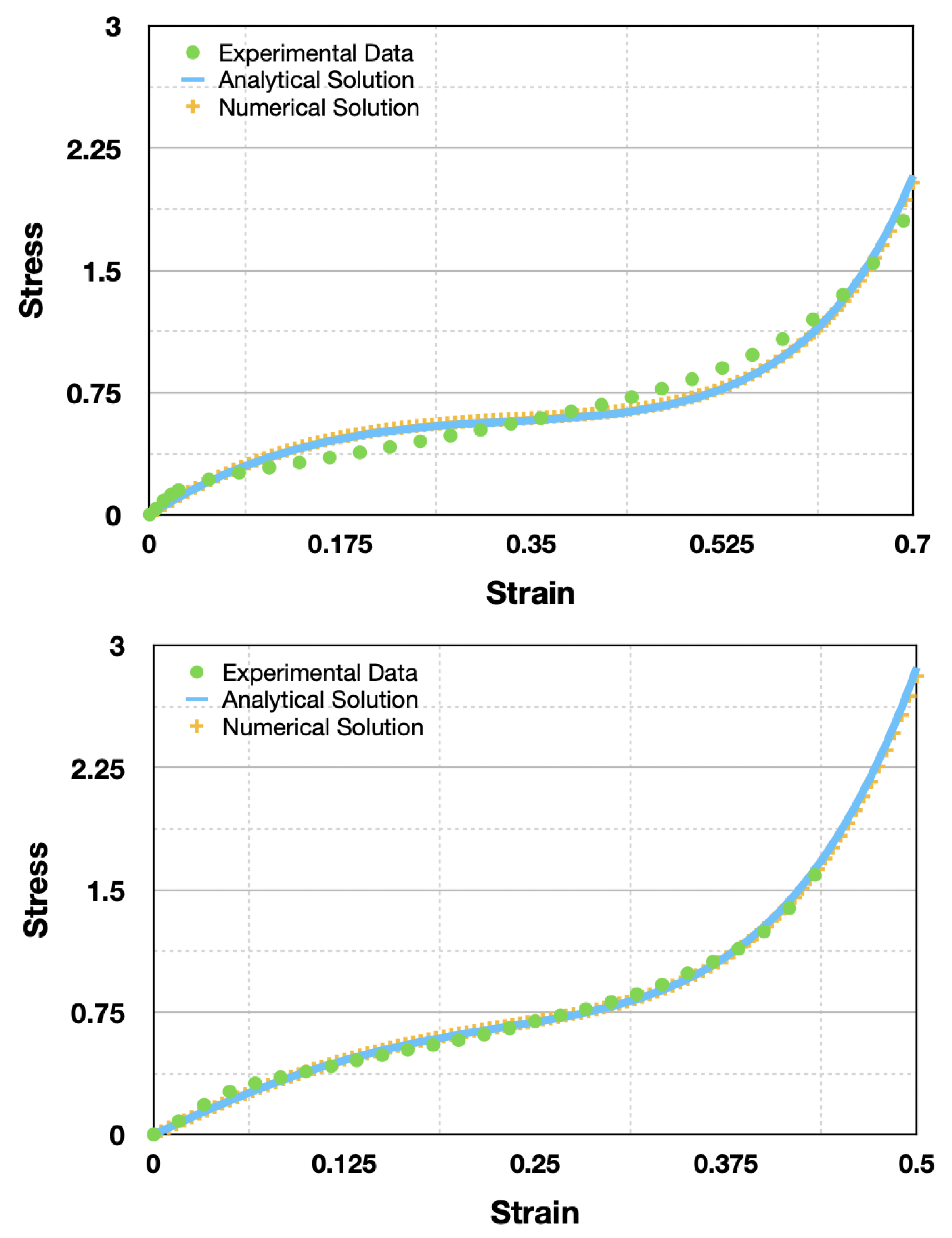
In Figure 7, we can see the results obtained for the two cases studied. From left to right, we can see the comparison between the numerical and analytical results of the equibiaxial and uniaxial tests. As expected, the equibiaxial test has a smaller plateau area and densification occurs earlier than in the uniaxial test.
These two simulations show that the agglomerated cork model presented represents with good accuracy the real behavior of the material, and therefore, it is a good option to be studied from now on.
8. Conclusions and Future Work
In this paper, we present a new material model for agglomerated cork. This model is based on the Mooney–Rivlin hyperelastic model and, as the cork agglomerate has a Poisson ratio near zero, has six material parameters. Analytical solutions for uniaxial and equibiaxial tests were developed and used for parameterization. To parameterize, the Nelder–Mead algorithm was used.
We also describe and use the successive linear approximation method (SLA) for the numerical simulation. The description of the SLA was quite general, and can be used for any material.
Our results show that the presented model is a good model and was validated through numerical simulation. One of the advantages of our model is the mathematical simplicity in relation to the classical model [16,17], being a direct extension of a Mooney–Rivlin model.
For future work, it will be interesting to try to relate the parameters , , , , and with physical parameters of the material, as was performed directly with the and the Poisson ratio. Another interesting approach to test the efficiency of the SLA will be the study of a contact-impact problem.
Author Contributions
Conceptualization, G.T.d.A.P., R.J.A.d.S., I.-S.L., M.G.T. and F.A.O.F.; methodology, G.T.d.A.P., R.J.A.d.S., I.-S.L., M.G.T. and F.A.O.F.; formal analysis, G.T.d.A.P., I.-S.L. and M.G.T.; investigation, G.T.d.A.P. and M.G.T.; resources, R.J.A.d.S., M.G.T. and F.A.O.F.; data curation, G.T.d.A.P.; writing—original draft preparation, G.T.d.A.P.; writing—review and editing, G.T.d.A.P., R.J.A.d.S., I.-S.L., M.G.T. and F.A.O.F.; visualization, I.-S.L. and F.A.O.F.; supervision, R.J.A.d.S., I.-S.L. and M.G.T.; project administration, M.G.T. All authors have read and agreed to the published version of the manuscript.
Funding
The author GTAP would like to thank Coordenação de Aperfeiçoamento de Pessoal de Nível Superior (CAPES) for their support (grant number 88881.188598/2018-01). The authors FAOF and RJAS acknowledge the support given by Fundação para a Ciência e a Tecnologia (FCT), through the projects UIDB/00481/2020 and UIDP/00481/2020. In addition, CENTRO-01-0145-FEDER-022083—Centro Portugal Regional Operational Programme (Centro2020) under the PORTUGAL 2020 Partnership Agreement through the European Regional Development Fund.
Data Availability Statement
All data is reported within the article.
Conflicts of Interest
The authors declare no conflict of interest.
References
- Dart, S.L.; Eugene, G. Elastic properties of cork. I. stress relaxation of compressed cork. J. Appl. Phys. 1946, 17, 314–318. [Google Scholar] [CrossRef]
- Anjos, O.; Pereira, H.; Rosa, M.E. Effect of quality, porosity and density on the compression properties of cork. Holz Als-Roh-Und Werkst. 2008, 66, 295–301. [Google Scholar] [CrossRef]
- Pereira, H.; Graça, J.; Baptista, C. The effect of growth-rate on the structure and compressive properties of cork. IAWA Bull. 1992, 13, 389–396. [Google Scholar] [CrossRef]
- Fortes, M.A.; Nogueira, M.T. The Poisson effect in cork. Mater. Sci. Eng. A 1989, 122, 227–232. [Google Scholar] [CrossRef]
- Delucia, M.; Catapano, A.; Montemurro, M.; Pailhes, J. Pre-stress state in cork agglomerates: Simulation of the compression moulding process. Int. J. Mater. Form. 2021, 14, 485–498. [Google Scholar] [CrossRef]
- Delucia, M.; Catapano, A.; Montemurro, M.; Pailhès, J. Determination of the effective thermoelastic properties of cork-based agglomerates. J. Reinf. Plast. Compos. 2019, 38, 760–776. [Google Scholar] [CrossRef]
- Rosa, M.E.; Osorio, J.; Gree, V. Torsion of cork under compression. Mater. Sci. Forum 2004, 455–456, 235–238. [Google Scholar] [CrossRef]
- Rosa, M.E.; Fortes, M.A. Deformation and fracture of cork in tension. J. Mater. Sci. 1991, 26, 341–348. [Google Scholar] [CrossRef]
- Castro, O.; Silva, J.M.; Devezas, T.; Silva, A.; Gil, L. Cork agglomerates as an ideal core material in lightweight structures. Mater. Des. 2010, 31, 425–432. [Google Scholar] [CrossRef] [Green Version]
- Sarasini, F.; Tirillò, J.; Lampani, L.; Sasso, M.; Mancini, E.; Burgstaller, C.; Calzolari, A. Static and dynamic characterization of agglomerated cork and related sandwich structures. Compos. Struct. 2019, 212, 439–451. [Google Scholar] [CrossRef]
- Ivañez, I.; Sánchez-Saez, S.; Garcia-Castillo, S.K.; Barbero, E.; Amaro, A.; Reis, P.N.B. High-velocity impact behaviour of damaged sandwich plates with agglomerated cork core. Compos. Struct. 2020, 248, 112520. [Google Scholar] [CrossRef]
- Lakreb, N.; Bezzazi, B.; Pereira, H. Mechanical strength properties of innovative sandwich panels with expanded cork agglomerates. Eur. J. Wood Wood Prod. 2015, 73, 46–473. [Google Scholar] [CrossRef]
- Sergi, C.; Tirillò, J.; Sarasini, F.; Barbero Pozuelo, E.; Sanchez-Saez, S.; Burgstaller, C. The Potential of Agglomerated Cork for Sandwich Structures: A Systematic Investigation of Physical, Thermal, and Mechanical Properties. Polymers 2019, 11, 2118. [Google Scholar] [CrossRef] [PubMed] [Green Version]
- Pernas-Sánchez, J.; Artero-Guerrero, J.A.; Varas, D.; Teixeira-Dias, F. Cork Core Sandwich Plates for Blast Protection. Appl. Sci. 2020, 10, 5180. [Google Scholar] [CrossRef]
- Gomez, A.; Barbero, E.; Sanchez-Saez, S. Modelling of carbon/epoxy sandwich panels with agglomerated cork core subjected to impact loads. Int. J. Impact Eng. 2022, 159, 104047. [Google Scholar] [CrossRef]
- Ogden, R.W. Large deformation isotropic elasticity – on the correlation of theory and experiment for incompressible rubberlike solids. Proc. R. Soc. Lond. Ser. A Math. Phys. Sci. 1972, 326, 565–584. [Google Scholar] [CrossRef]
- Hill, R. Aspects of invariance in solid mechanics. Adv. Appl. Mech. 1978, 18, 1–75. [Google Scholar]
- Delucia, M.; Catapano, A.; Montemurro, M.; Pailhés, J. A stochastic approach for predicting the temperature-dependent elastic properties of cork-based composites. Mech. Mater. 2020, 145, 103399. [Google Scholar] [CrossRef]
- Liu, I.-S.; Cipolatti, R.; Rincon, M.A. Sucessive Linear Approximation for Finite Elasticity. Comput. Appl. Math. 2010, 3, 465–478. [Google Scholar]
- Truesdell, C.; Noll, W. The Non-Linear Field Theories of Mechanics, 3rd ed.; Springer: Berlin, Germany, 2004. [Google Scholar]
- Liu, I.-S. Successive Linear Approximation for Boundary Value Problems of Nonlinear Elasticity in Relative-Descriptional Formulation. Int. J. Eng. Sci. 2011, 49, 635–645. [Google Scholar] [CrossRef]
- Liu, I.-S.; Cipolatti, R.; Rincon, M.A.; Palermo, L.A. Successive Linear Approximation for Large Deformation—Instability of Salt Migration. J. Elast. 2014, 114, 19–39. [Google Scholar] [CrossRef]
- Teixeira, M.G.; Liu, I.-S.; Rincon, M.A.; Cipolatti, R.A.; Palermo, L.A. The Influence of temperature on the formation of salt domes. Int. J. Model. Simul. Pet. Ind. 2014, 8, 35–41. [Google Scholar]
- Kossa, A.; Berezvai, S. Novel strategy for the hyperelastic parameter fitting procedure of polymer foam materials. Polym. Test. 2016, 53, 149–155. [Google Scholar] [CrossRef]
- Pereira, A.B.; Fernandes, F.A.O.; de Morais, A.B.; Maio, J. Biaxial Testing Machine: Development and Evaluation. Machines 2020, 8, 40. [Google Scholar] [CrossRef]
- Teixeira, M.G.; Pereira, G.T.A.; Liu, I.-S. Relative lagrangian formulation in thermo-viscoelastic solid bodies. Contin. Mech. Thermodunamics 2021, 33, 2263–2277. [Google Scholar] [CrossRef]
- Green, A.E.; Rivlin, R.S.; Shield, R.T. General theory of small elastic deformations superposed on finite deformations. Arch. Ration. Mech. Anal 1952, 211, 128–154. [Google Scholar]
Figure 1.
The deformation and deformation gradient diagram.

Figure 2.
Uniaxial and equibiaxial compression tests schemes.

Figure 3.
Agglomerated cork sample positioned for uniaxial compression testing at quasi-static strain rates.
Figure 3.
Agglomerated cork sample positioned for uniaxial compression testing at quasi-static strain rates.

Figure 4.
Dimensions of the octagon-shaped sample and the experimental setup for the equibiaxial compression tests.
Figure 4.
Dimensions of the octagon-shaped sample and the experimental setup for the equibiaxial compression tests.

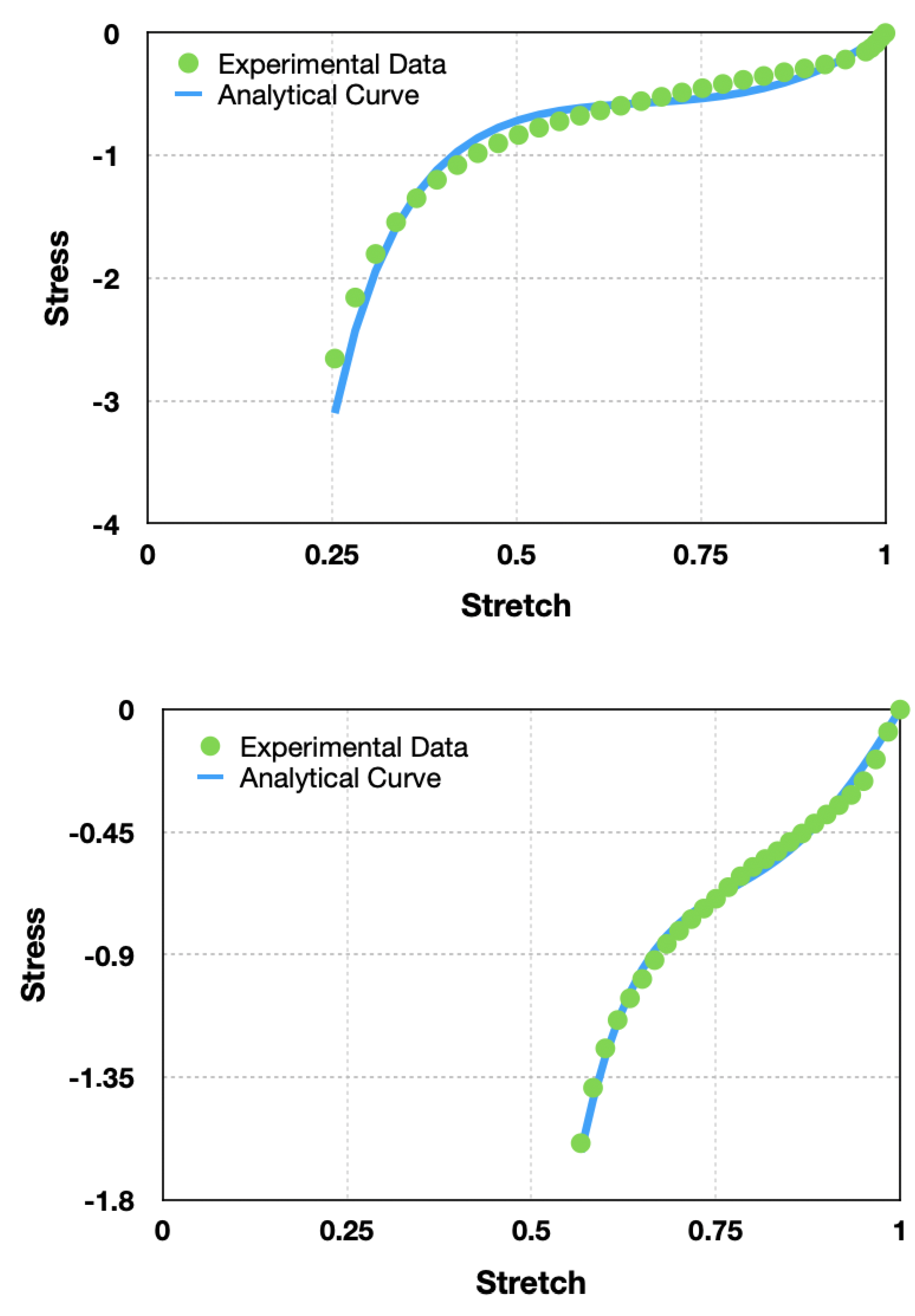
Figure 5.
Comparison between analytical and experimental results for uniaxial and equibiaxial tests, respectively.
Figure 5.
Comparison between analytical and experimental results for uniaxial and equibiaxial tests, respectively.

Figure 6.
Finite element mesh and boundary condition for both tests, uniaxial (left) and equibiaxial (right).
Figure 6.
Finite element mesh and boundary condition for both tests, uniaxial (left) and equibiaxial (right).

Figure 7.
Comparison between numerical, analytical and experimental solutions for uniaxial and equibiaxial compression tests, respectively.
Figure 7.
Comparison between numerical, analytical and experimental solutions for uniaxial and equibiaxial compression tests, respectively.


Table 1.
Values of experimental tests of uniaxial and equibiaxial compression.
| Uniaxial Compression | Equibiaxial Compression | ||
|---|---|---|---|
| Stretch | Stress [MPa] | Stretch | Stress [MPa] |
| 0.99990 | −0.00267 | 0.99983 | −0.00154 |
| 0.98716 | −0.08793 | 0.96683 | −0.18431 |
| 0.97331 | −0.15326 | 0.93350 | −0.31465 |
| 0.91794 | −0.25836 | 0.90016 | −0.38643 |
| 0.86256 | −0.32187 | 0.86683 | −0.45608 |
| 0.80718 | −0.38418 | 0.83350 | −0.52095 |
| 0.77949 | −0.41763 | 0.81683 | −0.54994 |
| 0.72411 | −0.48701 | 0.78350 | −0.61324 |
| 0.69642 | −0.52242 | 0.76683 | −0.65323 |
| 0.64104 | −0.59524 | 0.73350 | −0.73154 |
| 0.61335 | −0.63417 | 0.71683 | −0.77041 |
| 0.55797 | −0.72245 | 0.68350 | −0.86132 |
| 0.53028 | −0.77436 | 0.66683 | −0.92065 |
| 0.47490 | −0.90147 | 0.63350 | −1.06085 |
| 0.44721 | −0.98206 | 0.61683 | −1.14073 |
| 0.39183 | −1.19875 | 0.58350 | −1.38921 |
| 0.36414 | −1.34949 | 0.56683 | −1.59243 |
| 0.33645 | −1.54421 | ||
| 0.30876 | −1.80366 | ||
| 0.25339 | −2.65663 | ||
Table 2.
Obtained material parameters.
| Parameter | Value |
|---|---|
| −25.860100 | |
| 2.7356100 | |
| 19.317400 | |
| 0.0407647 | |
| −8.3524100 | |
| −2.5714300 |
Publisher’s Note: MDPI stays neutral with regard to jurisdictional claims in published maps and institutional affiliations. |
© 2022 by the authors. Licensee MDPI, Basel, Switzerland. This article is an open access article distributed under the terms and conditions of the Creative Commons Attribution (CC BY) license (https://creativecommons.org/licenses/by/4.0/).
Share and Cite
MDPI and ACS Style
Pereira, G.T.d.A.; Sousa, R.J.A.d.; Liu, I.-S.; Teixeira, M.G.; Fernandes, F.A.O. A New Material Model for Agglomerated Cork. Math. Comput. Appl. 2022, 27, 92. https://doi.org/10.3390/mca27060092
AMA Style
Pereira GTdA, Sousa RJAd, Liu I-S, Teixeira MG, Fernandes FAO. A New Material Model for Agglomerated Cork. Mathematical and Computational Applications. 2022; 27(6):92. https://doi.org/10.3390/mca27060092
Chicago/Turabian StylePereira, Gabriel Thomaz de Aquino, Ricardo J. Alves de Sousa, I-Shih Liu, Marcello Goulart Teixeira, and Fábio A. O. Fernandes. 2022. "A New Material Model for Agglomerated Cork" Mathematical and Computational Applications 27, no. 6: 92. https://doi.org/10.3390/mca27060092