Data-Driven Bayesian Network Learning: A Bi-Objective Approach to Address the Bias-Variance Decomposition

Abstract

We present a novel bi-objective approach to address the data-driven learning problem of Bayesian networks. Both the log-likelihood and the complexity of each candidate Bayesian network are considered as objectives to be optimized by our proposed algorithm named Nondominated Sorting Genetic Algorithm for learning Bayesian networks (NS2BN) which is based on the well-known NSGA-II algorithm. The core idea is to reduce the implicit selection bias-variance decomposition while identifying a set of competitive models using both objectives. Numerical results suggest that, in stark contrast to the single-objective approach, our bi-objective approach is useful to find competitive Bayesian networks especially in the complexity. Furthermore, our approach presents the end user with a set of solutions by showing different Bayesian network and their respective MDL and classification accuracy results.

1. Introduction

Bayesian Network (BN) [1] is a preferred formalism to represent knowledge under uncertainty using efficient reasoning. BN stands as a popular tool for prediction, diagnosis, decision-making, control, and to attain a better understanding of phenomena amenable to modeling. Nevertheless, building a BN comes with inherent difficulties, such as deciding on the specific graph structure, and corresponding parameter values. Two traditional ways to build a BN structure are through (i) domain expertise and (ii) a data-driven inductive approach. The induction of a BN from data is subsequently classified into two types (i) methods searching for conditional-dependencies, also known as constraint-based methods and (ii) search and scoring based methods [2,3,4,5]. This study is based on the latter case, where the learning task is framed as a combinatorial optimization problem with two main components: (1) a metric to assess the quality of each BN candidate, and (2) a search procedure to move intelligently through the space of candidate networks.

In data-driven BN learning, it is common to implement metrics in the form of a penalized log-likelihood (LL) function. LL is the log probability of the data given a network structure. While adding an edge to a BN never decreases the likelihood -and hence irrelevant edges may be added– adding extra edges leads to two main problems: the overfitting problem [6], where good performance in the training data comes with poor performance on the testing data and the construction of a densely connected network, which involves an increase in the running time and a poor description of the phenomenon being modelled when the network is being used for data analysis [7]. In order to deal with these problems, a penalty term is used to avoid complex networks. Such, complex networks may have a low LL score value but overfit the model while a high penalty term may incur in models that, on the other hand, underfit. The balance between the goodness of fit (measured as LL) and the complexity of a model is known as the bias-variance dilemma, decomposition or trade-off [8,9,10,11].

There are several decomposable penalized LL (DPLL) scoring functions for learning BN and are represented by the Akaike’s information criteria (AIC) [12], the Bayesian Dirichlet with score equivalence and uniforms priors (BDeu) [13], the factorized normalized maximum likelihood (fNML) [14], the Bayesian information criterion (BIC), and the minimum description length (MDL) [15]. These metrics differ mainly in their penalty function. Additionally, for the latest two cases, the MDL objective is to determine the model that provides the shortest description of the data set and, although the principles of BIC are different in the practice, some authors assure that MDL is simply the additive inverse of the BIC [5,16].

This work is based on crude MDL as the scoring metric, which is a popular metric used to learn BN structures [17,18,19,20,21]. Grünwald [15] defines the crude MDL as the two-part version of MDL, where “crude” means that the complexity of a model is calculated considering its parameters but not its functional form. Some researches consider that crude MDL is able to recover a network with a good bias-variance tradeoff; however, other works consider that this version of MDL is not complete and it will not work as expected [4,10,15,22]. Some researchers point out that to the trade-off between accuracy, measured in terms of the LL, and complexity should be featured as a multi-objective problem [23,24,25,26,27]; however, in the context of BN, the study of this approach has not been extensively studied. Motivated by this, our work addresses the comparison of a single-objective versus a multi-objective approach for learning BN from data. The single-objective Genetic algorithm (GA) uses crude MDL whereas NS2BN is used to find an appropriate selection of networks with a trade-off between accuracy and complexity.

The remainder of this paper is structured as follows: Section 2 describes related work and motivates the work conducted in this paper. In Section 3, the background is described. Section 4 describes our approach in detail. Section 5 presents the experiments setup. Section 6 discusses the results. The concluding section summarizes the findings and gives an account for future work.

2. Related Work

There exist two main approaches to the use of crude MDL to learn BN: (i) crude MDL to find the true model (that has given rise to the data), in our context it is the gold-standard network, and (ii) crude MDL to find a model with a good trade-off between the accuracy and complexity. Regarding the first approach, some of the most representative works are [4,28,29,30,31]. Regarding the second approach, some researchers assure that crude MDL is capable of finding a BN with a trade-off between the LL and the complexity, but not the gold-standard network [10,15,22,32,33]. As recent work in this approach, Cruz-Ramírez et al. [34], performed an exhaustive experiment with four-node networks. Therefore, even though these results show how crude MDL produces well-balanced models in terms of complexity and log-likelihood, those experiments have a limited scope and they left for future work to explore the search procedure, which is an important factor that affects the final selection of the model.

Previous studies have tackled the BN model selection problem using evolutionary algorithms. In [35] a Genetic Algorithm (GA) with genotype representation was proposed. The algorithm uses MDL as the fitness function and the results were based on evaluating several new recombination operators that helped to evolve BNs in a Directed Acyclic Graph (DAG) search space. In [36], the performance of GAs with two univariate Exploratory Data Analysis (EDA) based algorithms were compared. Three different scoring functions were used and the results showed that EDAs are able to recuperate structure similar to the gold-standard network. Wong’s works [37,38] are based on evolutionary programming to induce BN in a two-phase constraint-based method that yields models that predict more accurately in comparison with the previous work of Wong based on MDL as the fitness function. In [39], a novel algorithm based on immune binary particle swarm optimization and MDL as the fitness function was proposed. The experiments show advantages in the quality of the fitness function in a comparison between a Particle Swarm Optimization algorithm (PSO) and a GA. In [40], a hybrid algorithm between the maximal information coefficient and binary PSO was proposed. The experimental results show that without a given node ordering, this algorithm has better performance than the other five of the state of the art algorithms.

Lastly, the work of Ross and Zuviria [41] uses a multi-objective genetic approach to learn dynamic Bayesian networks from data with a trade-off between likelihood and complexity. This work is focused on the modeling of biological phenomena that typically require low-connectivity networks. However, to the best of our knowledge, this work is the only one with multi-objective criteria learning. Although, it is in the context of dynamic BN.

In summary, crude MDL uses a weighted sum to combine the log-likelihood and the structural complexity, thus, the learning problem of BN using MDL as a metric has been dealt mainly as a single-objective problem. However, we proved that one objective tends to dominate the search procedure and also add bias to the kind of result obtained [26].

3. Background

This section presents the main concepts that supports this investigation: the BN mathematical representation, the minimum description length principle, and the multi-objective problem.

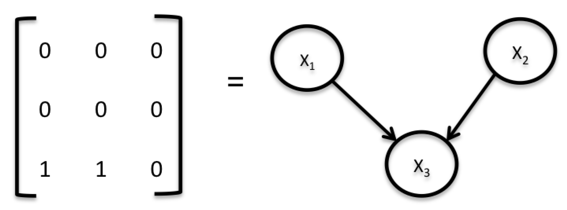
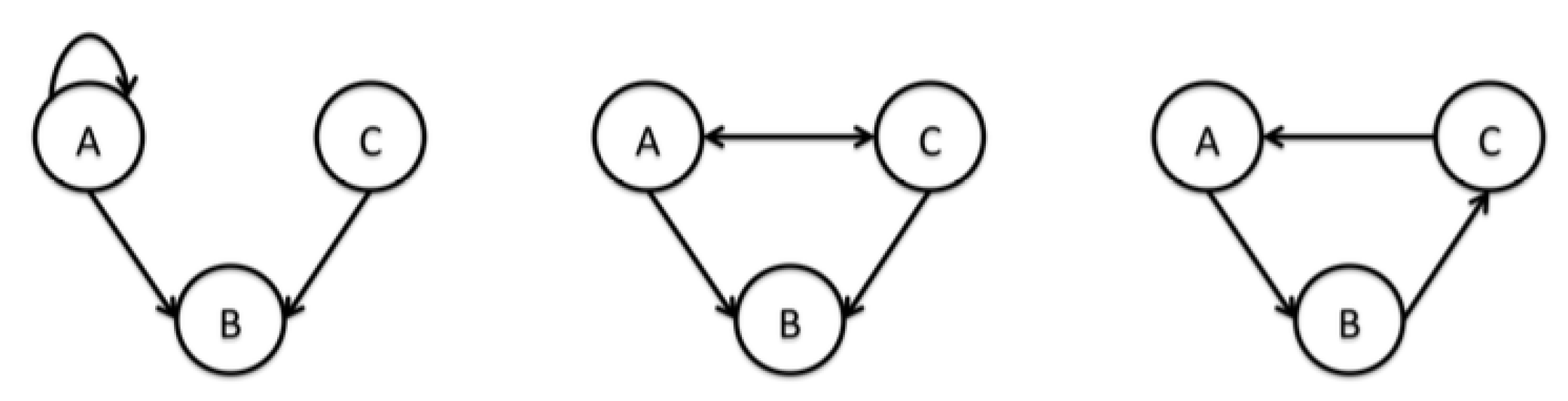
3.1. Bayesian Networks

A BN is a graphical model that represents a joint probability distribution over a set of random variables $\{X_1,\dots ,X_n\}$. BNs are represented as a pair $(G,\Theta )$, where the directed acyclic graph (DAG) is represented by $G=(U,E_G)$; U is the set of nodes or random variables, and $E_G$ is the set of arcs that represent the probabilistic relationship among these variables. The parents of $X_i$ are denoted $P{A}_i;X_i$ is independent of its non-descendant variables given its parents. Thus, $\Theta$ is a set of parameters which quantifies the network. The joint probability distribution can be recovered from local conditional probability distributions as is shown in Equation (1).

$$P\left(X_1,\dots ,X_n\right)=\prod _{i=1}^{n}P\left(X_i\right|P{A}_i)$$

(1)

Bayesian network structure learning is the problem of learning a network structure from dataset $\left(D\right)$, where the data set is a particular instantiation of all the variables $\{X_1,\dots ,X_n\}$. MDL is a well-known score used to measure the goodness of a BN candidate [15]. The model learned under the MDL principle is expected to exhibit a trade-off between model accuracy and complexity, thus avoiding data overfitting. In this work, the Bayesian learning problem is treated as a multi-objective optimization problem that consists of searching for potential solutions exhibiting a balanced trade-off between accuracy and the complexity (defined formally in the next subsection).

3.2. Minimum Description Length

The crude definition of MDL [15] is of the form:

$$MDL=-logP\left(D\right|\Theta )+\frac{k}{2}logn$$

(2)

$$k=\sum _{i=1}^m{q}_i(r_i-1)$$

(3)

where D is the dataset, $\Theta$ represents the parameters of the model, k is the dimension of the model, and n is the sample size. The parameter $\Theta$ is the corresponding local probability distribution for each node in the network. The dimension of the model (k) is given by Equation (3).

For the case of Equation (3), m is the number of variables, $q_i$ is the number of possible configurations of $P{A}_i$ and $r_i$ is the number of values of the variable.

The first term of Equation (2) measures the accuracy of the model using $-logP\left(D\right|\Theta )$ (represented as $f_1$ in the next section) and the second term measures the complexity using $\frac{k}{2}logn$ (represented as $f_2$ in the next section). The complexity of a BN is proportional to the number of arcs, as shown in Equation (3).

Hence, metrics that incorporate these two terms are dealing with a multi-objective problem which may represent that while the accuracy is better the complexity increases.

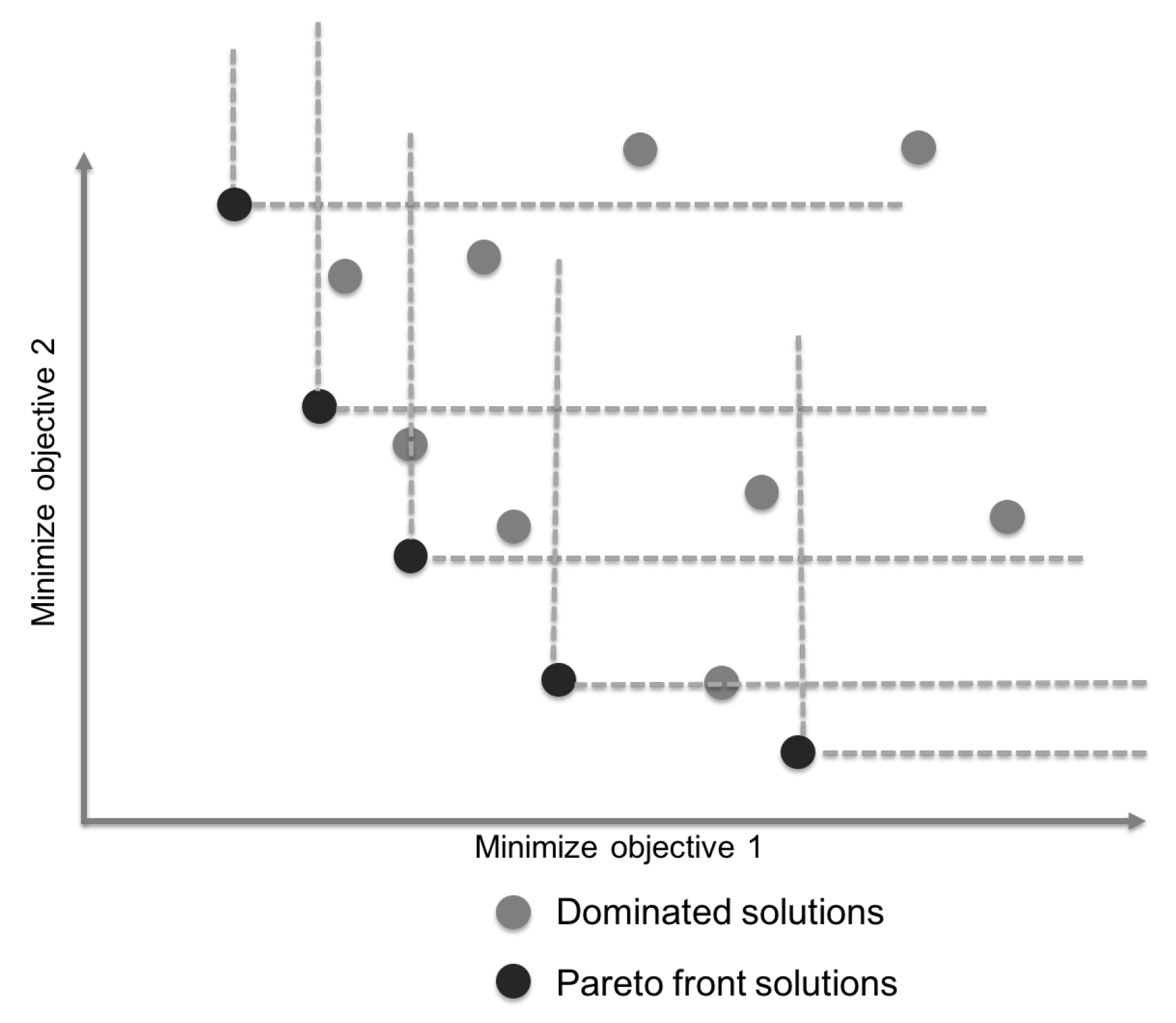
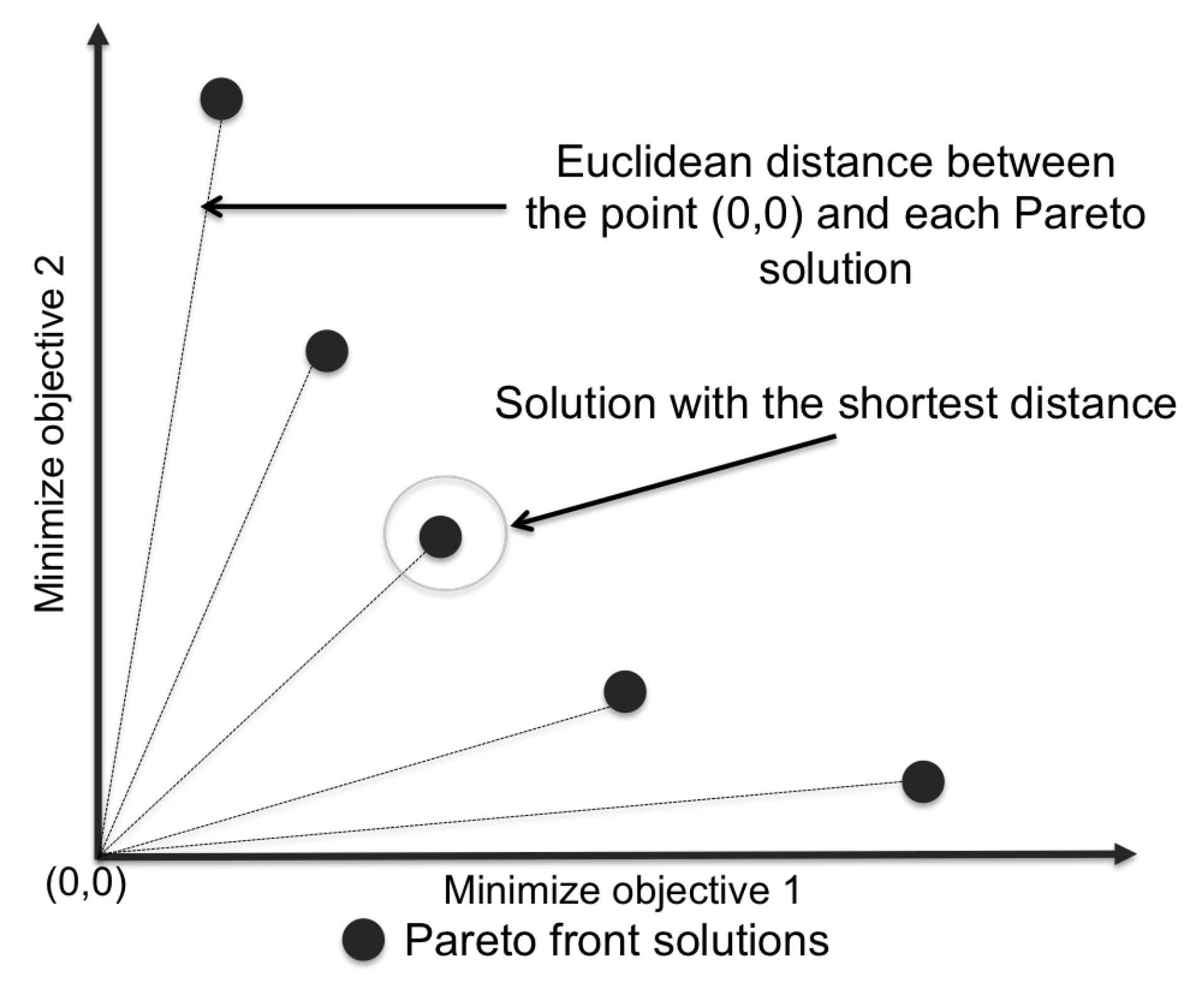
3.3. Multi-Objective Optimization Problem

According to Deb [42], a multi-objective optimization problem (MOOP) can be seen as a search problem that aims to minimize or maximize two (or more) objectives that are usually in conflict. Without loss of generality, a MOOP can be defined as: $\overrightarrow{f}\left(\overrightarrow{x}\right)=[f_1\left(\overrightarrow{x}\right),f_2\left(\overrightarrow{x}\right),\dots ,f_l\left(\overrightarrow{x}\right)]$ where $\overrightarrow{x}=[x_1,\dots ,x_n]\in R$ is an n-variable decision vector, $\overrightarrow{f}$ is the set of objective functions to be minimized or maximized, and l is the number of objectives (in our case, we have two objectives: the LL $f_1$ and the complexity $f_2$).

According to this idea, the following definitions are provided: a solution $x_1$ dominates a solution $x_2$ (denoted by $x_1⪯x_2$) if the solution $x_1$ is not worse than $x_2$ in all objectives and it is better than $x_2$ in at least one objective. In MOOPs there is not a single optimal solution; conversely, we can find a set of solutions that have no other solution which dominates them when all objectives are currently considered. Hence, the set of non-dominated solutions is called Pareto optimal set, and the evaluations of each non-dominated solution in each objective function are known as the Pareto front.

Figure 1 shows a particular case of the Pareto front in the presence of two-objective functions.

Several techniques have been proposed to solve MOOP [43]. This work is based on an evolutionary algorithm, which has shown advantages over classical techniques.

4. Nondominated Sorting Genetic Algorithm for Learning Bayesian Networks (NS2BN)

NSGA-II is a fast elitist multi-objective evolutionary algorithm proposed by Deb et al. [42]. In NSGA-II the individuals are ordered into non-dominated sets called fronts. In the first front are those individuals that are not dominated by the solutions in the current population. Such solutions are removed from the population and the process is repeated so as to select the set of non-dominated solutions to get the second front, and so on. A rank based on the number of the front is assigned to each individual. Additionally, the crowding distance is computed for each individual. The crowding distance is used to know how close an individual is to its neighbors in the objective function space. The selection of parents is performed by using binary tournament based on the rank and the crowding distance. The selected parents generate offsprings through crossover and mutation operators.

This work presents a multi-objective approach by using NSGA-II. The aim is to deal with the BN learning structure problem as a multi-objective optimization problem. The likelihood and the complexity of the model are considered as the objectives to be optimized. The pseudocode of the proposed approach NS2BN is presented in the Algorithm 1.

Algorithm 1: NS2BN

1:  G = 0 {Generation}

2:  Generate a population P of random solutions $\overrightarrow{x_i},\forall i,i=1,\dots ,POP\_SIZE$

3:  Repair cycles of each ${\overrightarrow{x}}_i\forall i,i=1,\dots ,POP\_SIZE$

4:  Evaluate the fitness functions using the first and the second term of the Equation (2) of each ${\overrightarrow{p}}_i\forall i,i=1,\dots ,POP\_SIZE$

5:  while $G\le G_{max}$ do

6:   Create an offspring population Q using: binary tournament selection, one-point crossover and bit inversion mutation.

7:   Repair cycles

8:   Evaluate the fitness functions using the first and the second term of the Equation (2) of each ${\overrightarrow{x}}_i\forall i,i=1,\dots ,POP\_SIZE$

9:   Combine parents and offspring populations $R=P\cup Q$

10:   Sort using non-dominated criterio

11:   Replacement

12:   $G=G+1$

13:  end while

For the implementation of NS2BN, the following features are highlighted, (i) due to the nature of the problem, the representation of individuals (BNs) is an adjacency matrix as can be seen in Figure 2, (ii) due to this representation, a repair operator to avoid cycles inspired on [44] is used (see Figure 3). This repair operator identifies cycles in three kinds of processes: self-cycles, by-cycles, and regular cycles. In the first one, the repair strategy is to replace the value along the diagonal, when the value is 1 by 0. The second repair strategy fixes the bi-directional cycles that occurs when two nodes are seen to influence each other then the repair operator removes one of the arcs at random to resolve it; finally the regular cycles need to identify a path between nodes, the strategy is the same as the path-cyclic graphs, where one of the offending arcs is removed randomly. And, (iii) the fitness functions are defined by each term of Equation (2) and both are minimizations.

Regarding the total computational cost per iteration; to the cost of the base algorithm we add the cost of the repair operator, therefore our NS2BN algorithm is $\mathcal{O}\left(M{N}^2\right)+\mathcal{O}\left(ND\right)$, where; M is the number objectives, N is the population size and D is the dimensionality of the individuals [42].

5. Experimental Setup

This section presents the experimental setup used to compare the resultant BN models in terms of the trade-off between LL and complexity. A set of twelve databases was used: (i) four synthetic databases with 6-nodes, in which all the random variables are binary; do not produce any qualitative impact on the results in comparison to non-binary variables [45]. Two of these databases were generated using a random probability distribution and the next two were generated with distribution $p=0.1$ that according to [45] changing the parameters to be high or low tends to produce low-entropy distributions which have more potential for data compression. Tetrad IV software [46] was used to generate synthetic databases with a specific distribution. (ii) Three databases of a well-known benchmark [47] and (iii) five databases from the UCI repository [48].

Table 1. Databases used in the experiments.

No.	Name	Attributes	Instances	Arcs
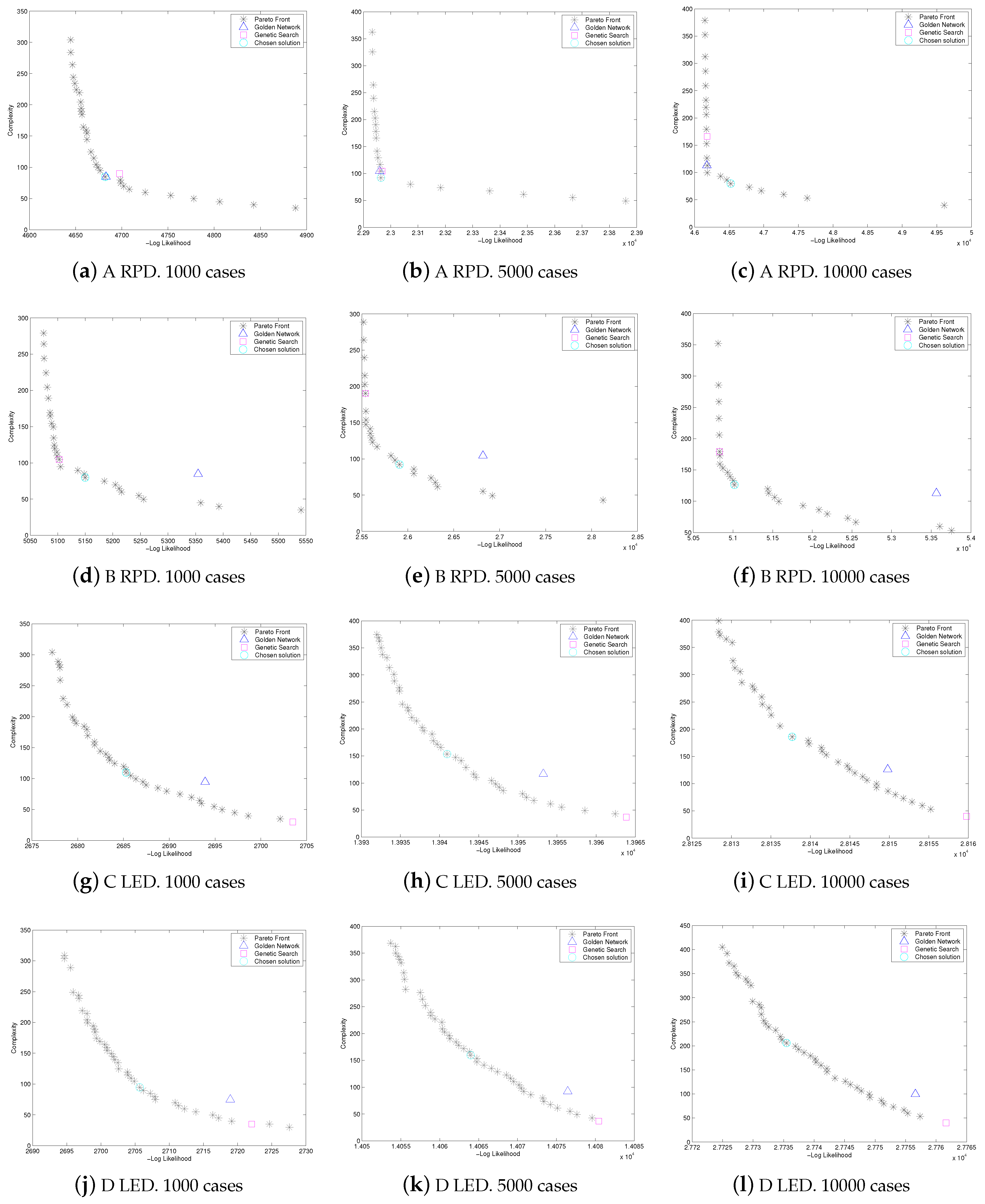
1.	A6 Nodes-random probability distribution	6	1000, 5000, 10000	8
2.	B6 Nodes-random probability distribution	6	1000, 5000, 10000	8
3.	C6 Nodes-low entropy probability distribution	6	1000, 5000, 10000	9
4.	D6 Nodes-low entropy probability distribution	6	1000, 5000, 10000	7
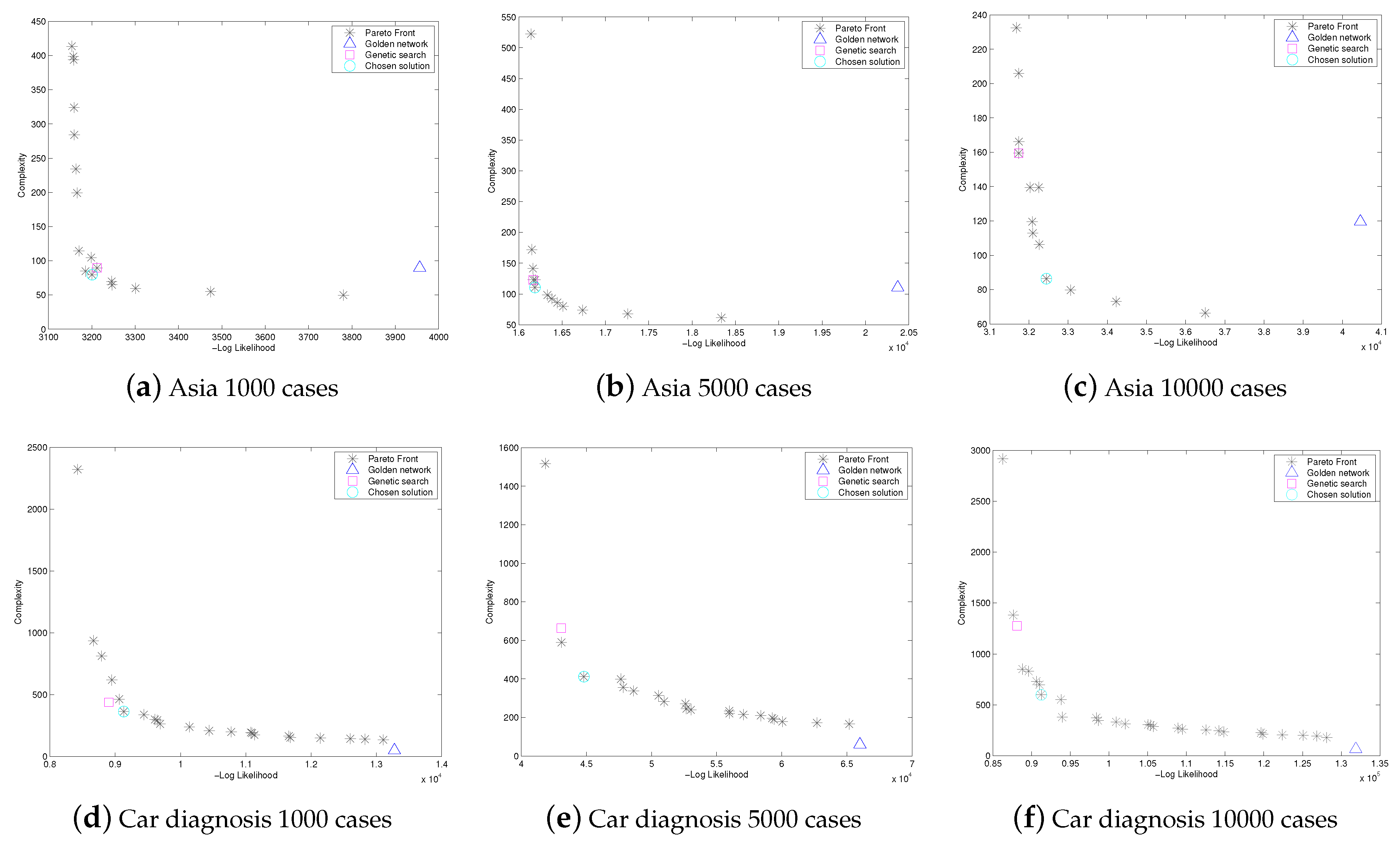
5.	Asia	8	1000, 5000, 10000	8
6.	Car Diagnosis	18	1000, 5000, 10000	20
7.	Child	20	1000, 3000	Unknown
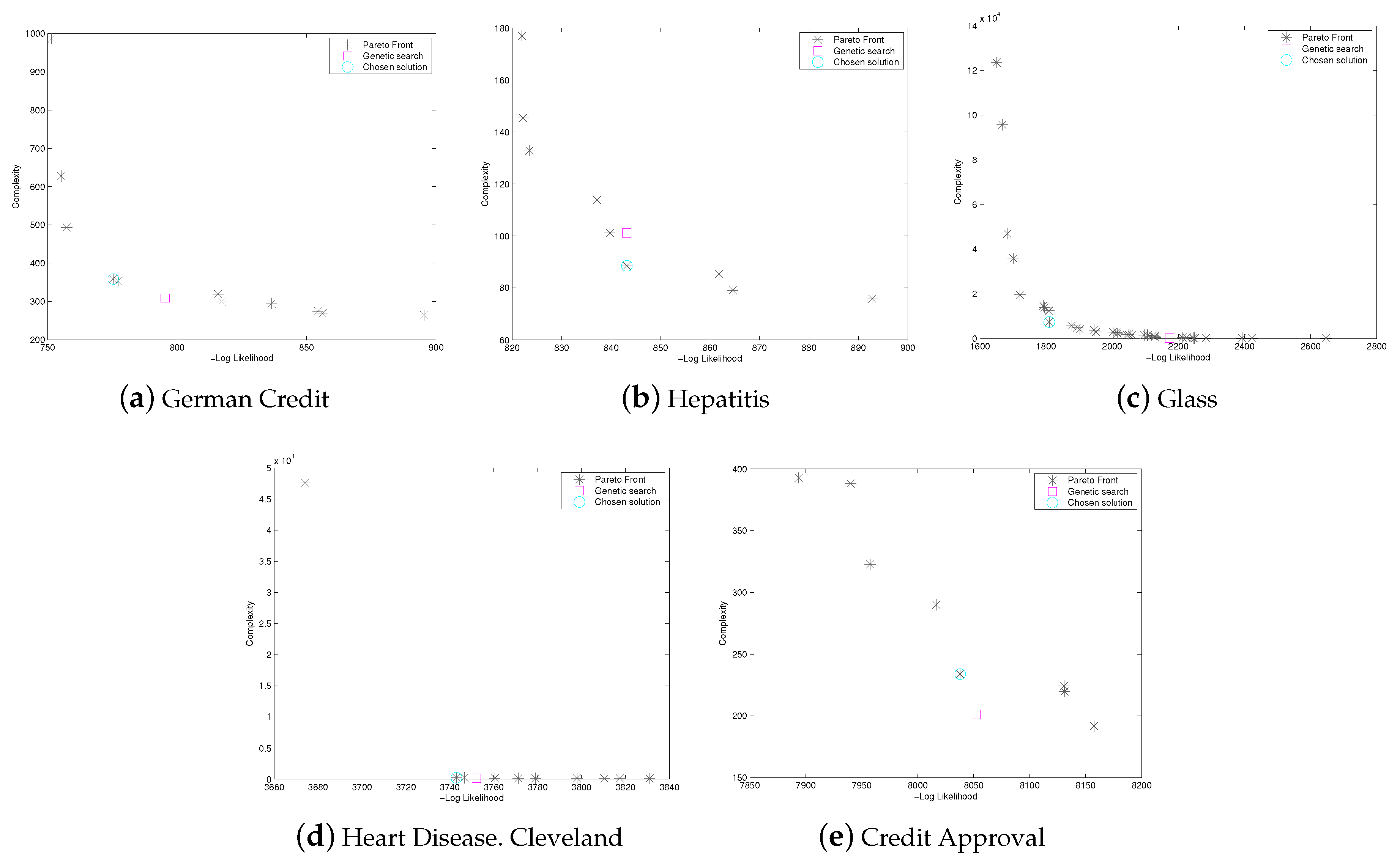
8.	German Credit	21	1000	Unknown
9.	Hepatitis	20	80	Unknown
10.	Glass	10	270	Unknown
11.	Heart Disease. Cleveland	14	298	Unknown
12.	Credit Approval	16	654	Unknown

shows a detailed description of each database.

A single objective Genetic Algorithm [49] (GABN) was adopted for comparison purposes. The individual representation consists of the same adjacency matrix above discussed; the fitness function is the crude MDL, as described in the previous Section 3.2. In this algorithm, binary tournament parent selection, one-point crossover and bit inversion mutation are employed.

Ten independent runs were made by each algorithm per database, with 20,000 evaluations each. The GABN finds a single network for each execution, the network with the best MDL is chosen as the “genetic solution”, meanwhile, in NS2BN the result of a run is a set of solutions with a variety of accuracy and structural complexity measurements. Based on the fact that all solutions in the Pareto front are optima, a decision making process based on expert knowledge in the modeling field is required to choose the most suitable solution.

To carry out a comparison between the multi-objective approach and the single-objective approach the linear programming technique for multidimensional analysis of preference (LINMAP) was used [50]. In the LINMAP decision approach criterion, from the accumulated Pareto front of ten executions, the solution nearest to a reference point which is (0, 0) is chosen. To find this solution all the solutions were normalized and the Euclidean distances were computed between the reference point and each Pareto solution as is shown in Figure 4. The solution with the shortest Euclidean distance is referred to as the chosen solution in this work.

The experimentation is presented in three parts: (1) the chosen solution obtained by NS2BN and the single solution from the Genetic algorithm are compared in terms of their complexity, likelihood, MDL and the classification accuracy using 10-fold-cross-validation (See Equation (5), where CV is test error on kth fold), (2) for the case of the databases in Table 1 from 1 to 6, we measure how the probability distribution of the gold-standard network is different from the genetic solution; for this computation the formulation of the Kullback Leibler distance (KLD) was used, see Equation (4). Finally, (3) the analysis of the plots of the accumulated Pareto fronts are discussed.

$$D_{KL}\left(p\right|\left|q\right)=\sum _{i=0}^N\left(x_i\right)lo{g}_2\left(\frac{p\left(x_i\right)}{q\left(x_i\right)}\right)$$

(4)

where $q\left(x\right)$ is the approximation and $p\left(x\right)$ is the gold-standard network distribution that we are interested in matching $q\left(x\right)$. If the obtained value is equal to 0 means that the distributions perfectly match, otherwise, it can take values between 0 and ∞.

$$CV=\frac{1}{K}\sum _{k=1}^{K}C{V}_k$$

(5)

The parameter setting employed by NS2BN and the GA were tuning empirically. The parameters are as follows: $POP\_SIZE$ = 100, $G_{max}$ = 200, C = 0.9 and M = 0.3.

6. Results

Table 2. Comparison between the NS2BN and the GABN solutions. Values in parentheses represent the standard deviation, for the case of -Log-Likelihood, complexity, and MDL the minimum value is in boldface. For the case of the CV, we carry out the t-test and values in boldface mean the significant best value found.

Model	Trade-off		MDL	CV
	−Log Likelihood	Complexity
A6-Nodes random probability distribution. 1000 cases
Chosen solution	4682.057654	84.70916642	4766.76682	71.25(±3.25)
Genetic solution	4697.44594	89.69205856	4787.137998	72.10(±2.86)
A6-Nodes random probability distribution. 5000 cases
Chosen solution	22964.2851	92.15784285	23056.44294	72.42(±1.55)
Genetic solution	22968.59399	104.4455552	23073.03954	71.88(±1.93)
A6-Nodes random probability distribution. 10000 cases
Chosen solution	46522.66474	79.72627428	46602.39101	70.37(±0.76)
Genetic solution	46181.77888	166.0964047	46347.87529	70.29(±0.81)
B6-Nodes random probability distribution. 1000 cases
Chosen solution	5149.786108	79.72627428	5229.512382	85.59(±3.32)
Genetic solution	5102.720574	104.640735	5207.361309	85.75(±3.34)
B6-Nodes random probability distribution. 5000 cases
Chosen solution	25909.78695	92.15784285	26001.94479	83.58(±1.45)
Genetic solution	25540.93739	190.4595419	25731.39693	84.23(±1.41)
B6-Nodes random probability distribution. 10000 cases
Chosen solution	51018.73479	126.2332676	51144.96806	84.62(±0.96)
Genetic solution	50830.79577	179.3841171	51010.17989	84.71(±0.98)
C6-Nodes low-entropy probability distribution. 1000 cases
Chosen solution	2685.283382	109.6236271	2794.907009	89.70(±0.54)
Genetic solution	2703.478277	29.89735285	2733.37563	89.60(±0.49)
C6-Nodes low-entropy probability distribution. 5000 cases
Chosen solution	13940.96186	153.5964047	14094.55826	90.22(±0.09)
Genetic solution	13963.84415	36.86313714	14000.70728	90.24(±0.08)
C6-Nodes low-entropy probability distribution. 10000 cases
Chosen solution	28137.70083	186.0279733	28323.7288	90.21(±0.03)
Genetic solution	28159.77242	39.86313714	28199.63556	90.21(±0.03)
D6-Nodes low-entropy probability distribution. 1000 cases
Chosen solution	2705.676276	94.6749507	2800.351227	91.40(±0.49)
Genetic solution	2722.059767	34.880245	2756.940012	91.40(±0.49)
D6-Nodes low-entropy probability distribution. 5000 cases
Chosen solution	14063.96978	159.7402609	14223.71004	90.76(±0.08)
Genetic solution	14080.43878	36.86313714	14117.30192	90.76(±0.08)
D6-Nodes low-entropy probability distribution. 10000 cases
Chosen solution	27735.47963	205.9595419	27941.43917	90.27(±0.05)
Genetic solution	27761.63739	39.86313714	27801.50053	90.27(±0.05)
Asia. 1000 cases
Chosen solution	3200.726031	79.72627428	3280.452306	94.30(±1.87)
Genetic solution	3211.984813	89.69205856	3301.676872	94.30(±1.87)
Asia. 5000 cases
Chosen solution	16188.02485	110.5894114	16298.61427	94.10(±0.81)
Genetic solution	16167.19634	122.8771238	16290.07347	94.10(±0.81)
Asia. 10000 cases
Chosen solution	32444.35458	86.37013047	32530.72471	94.12(±0.52)
Genetic solution	31738.67533	159.4525486	31898.12788	94.12(±0.52)
Car diagnosis. 1000 cases
Chosen solution	9130.727267	363.7511264	9494.478394	71.10(±0.30)
Genetic solution	8903.130665	438.4945085	9341.625174	69.33(±1.52)
Car diagnosis. 5000 cases
Chosen solution	44811.82111	411.6383647	45223.45948	75.10(±1.64)
Genetic solution	43066.63622	663.5364685	43730.17269	76.12(±1.86)
Car diagnosis. 10000 cases
Chosen solution	91244.39425	597.9470571	91842.34131	76.76(±1.34)
Genetic solution	88106.54485	1275.620388	89382.16524	72.44(±1.46)
German Credit
Chosen solution	775.3134767	358.7682342	1134.081711	70.00(±0.00)
Genetic solution	795.3572652	308.9393128	1104.296578	70.00(±0.00)
Hepatitis
Chosen solution	843.1819384	88.50699333	931.6889318	83.75(±5.76)
Genetic solution	843.1298695	101.1508495	944.280719	83.75(±5.76)
Glass
Chosen solution	1809.775474	7335.03997	9144.815443	76.58(±7.29)
Genetic solution	2174.033877	170.3122737	2344.346151	35.51(±2.08)
Heart Disease. Cleveland
Chosen solution	3743.020428	250.5367332	3993.557162	56.89(±5.06)
Genetic solution	3752.086989	151.9649037	3904.051893	53.89(±0.85)
Credit Approval
Chosen solution	8037.915455	233.7734795	8271.688934	72.90(±5.29)
Genetic solution	8052.242078	201.0451924	8253.287271	60.49(±5.03)

shows the results in terms of LL, complexity, and MDL for the chosen solution and the genetic solution. Additionally, the results in terms of the 10-fold-cross-validation rate are presented in the column named “CV”. A parametric t-test with $95\%$-confidence was applied between the chosen solution and the genetic solution in terms of classification accuracy. Numbers in bold-face letters indicate that the difference between accuracies is significant and this accuracy is the best.

According to such a test, in five databases there were significant differences in favor of the NS2BN chosen solution. The rest of the results did not show significant differences, which means that genetic solutions do not have advantages or disadvantages in terms of classification. Since the genetic algorithm is searching the minimum value of MDL, the genetic solutions show a minor MDL in sixteen databases. However, one of the objectives is clearly affected in those results.

Figure 5d–f show how the genetic solution tends to choose solutions with a smaller log-likelihood but more complex, and a similar situation occurs in Figure 5g–i where the GABN chooses solutions less complex but with a worse log-likelihood value.

It is important to notice the prominence of the search procedure and all the elements associated with this. It may be necessary, in the case where the genetic algorithm tends to choose solutions with a smaller LL but more complex, to find the balance in the configuration parameters to have a balance between exploration and exploitation. Other components that could be explored include genetic diversity, reinitialization, or self-adaptation, which we will leave for future work.

Regarding the sample size, Grünwald [15] points that crude MDL does not work well when the sample size is small or moderate and Hastie et al. [16] point out that a metric like crude MDL, in a finite sample, tends to select less complex models. Our results agree with Grünwald and in contrast to Hastie’s et al, our work shows a bias when the sample size is greater in the Genetic Solution, which is used a weighted sum, since this solution tends to select a more complex model (see Figure 5b,c,e,f, Figure 6f and Figure 7b,c).

The experiments generated by a low-entropy distribution show, as was pointed by Cruz-Ramírez et al. [34] that the presence of noise rate affects the behavior of MLD, which tends to prefer the less complex models, even a network with no arcs. However, the results of the experiments with low entropy distribution show, regardless the sample size, solutions with better values in both terms in comparison with the solution provided by NS2BN (see Figure 5g–l).

Finally,

Table 3. Kullback–Leibler divergence computed between the gold-standard network with the GABN solution and the gold-standard network with the chosen solution of the NS2BN Pareto front. Values in boldface mean the best value found.

Golden-Network	GABN	NS2BN
A RPD. 1000 cases	0.006256036	0.000412874
A RPD. 5000 cases	0.000735484	0.000166667
A RPD. 10000 cases	0.000622825	0.010558429
B RPD. 1000 cases	0.5008542	0.512832286
B RPD. 5000 cases	0.50817743	0.527715617
B RPD. 10000 cases	0.501635069	0.506660672
C LED. 1000 cases	0.006859061	0.000558415
C LED. 5000 cases	0.001254388	8.84927E-06
C LED. 10000 cases	0.000630321	0.000231126
D LED. 1000 cases	0.005505678	0.001674059
D LED. 5000 cases	0.001196043	0.0007695
D LED. 10000 cases	0.000561088	0.000529102
Asia 1000 cases	0.184669176	0.183903387
Asia 5000 cases	0.279944777	0.277977466
Asia 10000 cases	0.272191288	0.262362486
Car diagnosis 1000 cases	0.161505741	0.278079726
Car diagnosis 5000 cases	0.160725004	0.192815203
Car diagnosis 10000 cases	0.200548739	0.223971025

shows the results of the KLD computation. According to such a test, there were significant differences in ten databases in favor of the solution obtained by NS2BN, which means that the chosen solution is closest to the gold-standard network concerning the underlying distribution.

7. Conclusions and Future Work

In this paper, a novel evolutionary bi-objective optimization approach for model selection of BN was presented. The accuracy and the complexity, which are related to bias and variance respectively, were adopted as the objectives to be optimized so as to obtain models with an acceptable generalization performance. A set of trade-off solutions was obtained per database. A solution nearest to the origin was chosen as a competitive solution with a suitable trade-off between the objectives. This chosen solution was compared with a single-objective solution. The chosen solution achieved competitive results, especially in complexity. It is important to note, that one of the main advantages of this approach is the set of trade-off solutions and that the selection of a model can be a high-level decision and must be performed by a domain expert of the modeling phenomenon. Additional advantages are that the proposed method can be applied to a databases from different domains and can be extended to other models such as artificial neural networks. As future work, different methods can be used to control (adapt or self-adapt) the algorithms parameters. Also, alternatives to reduce the computational cost of the algorithm can be included.

References

- Pearl, J. Bayesian networks: A model of self-activated memory for evidential reasoning. In Proceedings of the 7th Conference of the Cognitive Science Society, Irvine, CA, USA, 15–17 August 1985; pp. 329–334. [Google Scholar]
- Buntine, W. A Guide to the Literature on Learning Probabilistic Networks from Data. IEEE Trans. Knowl. Data Eng. 1996, 8, 195–210. [Google Scholar] [CrossRef] [Green Version]
- Rónán, D.; Qiang, D.; Stuart, A. Learning Bayesian networks: Approaches and issues. Knowl. Eng. Rev. 2011, 26, 99–157. [Google Scholar]
- Heckerman, D. A Tutorial on Learning with Bayesian Networks. In Learning in Graphical Models; Jordan, M.I., Ed.; MIT Press: Cambridge, MA, USA, 1999; pp. 301–354. [Google Scholar]
- Neapolitan, R.E. Learning Bayesian Networks; Prentice-Hall, Inc.: Upper Saddle River, NJ, USA, 2003. [Google Scholar]
- Domingos, P. Bayesian Averaging of Classifiers and the Overfitting Problem. In Proceedings of the 17th International Conference on Machine Learning, Stanford, CA, USA, 29 June–2 July 2000; pp. 223–230. [Google Scholar]
- Liu, Z.; Malone, B.; Yuan, C. Empirical Evaluation of Scoring Functions for Bayesian Network Model Selection. In Proceedings of the Ninth Annual MCBIOS Conference, Oxford, MS, USA, 17–18 February 2012; pp. 1–16. [Google Scholar]
- Geman, S.; Bienenstock, E.L.; Doursat, R. Neural Networks and the Bias/Variance Dilemma. Neural Comput. 1992, 4, 1–58. [Google Scholar] [CrossRef]
- Friedman, J.H. On Bias, Variance, 0’/1 Loss, and the Curse-of-Dimensionality. Data Min. Knowl. Discov. 1997, 1, 55–77. [Google Scholar] [CrossRef]
- Myung, I.J. The Importance of Complexity in Model Selection. J. Math. Psychol. 2000, 44, 190–204. [Google Scholar] [CrossRef] [PubMed] [Green Version]
- Hastie, T.; Tibshirani, R.; Friedman, J. Model Assessment and Selection. In The Elements of Statistical Learning; Springer New York Inc.: New York, NY, USA, 2001; pp. 219–227. [Google Scholar]
- Akaike, H. Information Theory and an Extension of the Maximum Likelihood Principle. In Selected Papers of Hirotugu Akaike; Springer: New York, NY, USA, 1998; pp. 199–213. [Google Scholar] [CrossRef]
- Cooper, G.F.; Herskovits, E. A Bayesian Method for the Induction of Probabilistic Networks from Data. Mach. Learn. 1992, 9, 309–347. [Google Scholar] [CrossRef]
- Silander, T.; Roos, T.; Myllymäki, P. Learning locally minimax optimal Bayesian networks. Int. J. Approx. Reason. 2010, 51, 544–557. [Google Scholar] [CrossRef] [Green Version]
- Grünwald, P.D. The Minimum Description Length Principle. Adaptive Computation and Machine Learning. In The Minimum Description Length Principle. Adaptive Computation and Machine Learning; The MIT Press: Cambridge, MA, USA, 2007; p. 703. [Google Scholar]
- Hastie, T.; Tibshirani, R.; Friedman, J. Unsupervised Learning. In The Elements of Statistical Learning; Springer: New York, NY, USA, 2001; p. 533. [Google Scholar]
- Ye, S.; Cai, H.; Sun, R. An Algorithm for Bayesian Networks Structure Learning Based on Simulated Annealing with MDL Restriction. In Proceedings of the 2008 Fourth International Conference on Natural Computation, Jinan, China, 18–20 October 2008; Volume 3, pp. 72–76. [Google Scholar]
- Kuo, S.; Wang, H.; Wei, H.; Chen, C.; Li, S. Applying MDL in PSO for learning Bayesian networks. In Proceedings of the 2011 IEEE International Conference on Fuzzy Systems (FUZZ-IEEE 2011), Taipei, Taiwan, 27–30 June 2011; pp. 1587–1592. [Google Scholar]
- Suzuki, J. Bayesian Network Structure Estimation Based on the Bayesian/MDL Criteria When Both Discrete and Continuous Variables Are Present. In Proceedings of the 2012 Data Compression Conference, Snowbird, UT, USA, 10–12 April 2012; pp. 307–316. [Google Scholar]
- Zhong, X.; You, W. Combining MDL and BIC to Build BNs for System Reliability Modeling. In Proceedings of the 2015 2nd International Conference on Information Science and Security (ICISS), Seoul, Korea, 14–16 December 2015; pp. 1–4. [Google Scholar]
- Chen, C.; Yuan, C. Learning Diverse Bayesian Networks. In Proceedings of the AAAI Conference on Artificial Intelligence, Honolulu, HI, USA, 27 January–1 February 2019; Volume 33, pp. 7793–7800. [Google Scholar]
- Grünwald, P.D. Model Selection Based on Minimum Description Length. J. Math. Psychol. 2000, 44, 133–152. [Google Scholar] [CrossRef] [PubMed]
- Liu, G.; Kadirkamanathan, V. Learning with multi-objective criteria. In Proceedings of the Fourth International Conference on Artificial Neural Networks, Cambridge, UK, 26–28 June 1995; pp. 53–58. [Google Scholar]
- Braga, A.P.; Takahashi, R.H.C.; Costa, M.A.; Teixeira, R.d.A. Multi-Objective Algorithms for Neural Networks Learning. In Multi-Objective Machine Learning; Springer: Berlin/Heidelberg, Germany, 2006; pp. 151–171. [Google Scholar] [CrossRef]
- Gräning, L.; Jin, Y.; Sendhoff, B. Generalization improvement in multi-objective learning. In Proceedings of the International Joint Conference on Neural Networks, Vancouver, BC, Canada, 16–21 July 2006; pp. 9893–9900. [Google Scholar]
- Yaman, S.; Lee, C.H. A Comparison of Single- and Multi-Objective Programming Approaches to Problems with Multiple Design Objectives. J. Signal Process. Syst. 2010, 61, 39–50. [Google Scholar] [CrossRef]
- Rosales, A.; Escalante, H.J.; Gonzalez, J.A.; Reyes, C.A.; Coello, C.A. Bias and Variance Optimization for SVMs Model Selection. In Proceedings of the Iberian Conference on Pattern Recognition and Image Analysis, Madeira, Portugal, 5–7 June 2013; pp. 108–116. [Google Scholar]
- Bouckaert, R.R. Probabilistic Network Construction Using the Minimum Description Length Principle. In Proceedings of the European Conference on Symbolic and Quantitative Approaches to Reasoning and Uncertainty, Granada, Spain, 8–10 November 1993. [Google Scholar]
- Lam, W.; Bacchus, F. Learning Bayesian Belief Networks: An Approach Based on the MDL Principle. Comput. Intell. 1994, 10, 269–293. [Google Scholar] [CrossRef] [Green Version]
- Suzuki, J. Learning Bayesian Belief Networks Based on the Minimum Description Length Principle: An Efficient Algorithm Using the B & B Technique. In Proceedings of the Thirteenth International Conference on International Conference on Machine Learning, Bari, Italy, 3–6 July 1996; pp. 462–470. [Google Scholar]
- Suzuki, J. Learning Bayesian Belief Networks Based on the Minimum. Description Length Principle: Basic Properties. IEICE Trans. Fundam. Electron. Commun. Comput. Sci. 1999, E82-A, 2237–2245. [Google Scholar]
- Grünwald, P.D. A Tutorial Introduction to the Minimum Description Length Principle. In Advances in Minimum Description Length: Theory and Applications; The MIT Press: Cambridge, MA, USA, 2005. [Google Scholar]
- Zou, Y.; Roos, T.; Ueno, M. On Model Selection, Bayesian Networks, and the Fisher Information Integral. In Advanced Methodologies for Bayesian Networks; Springer International Publishing: Cham, Switzerland, 2015; pp. 122–135. [Google Scholar] [CrossRef]
- Cruz-Ramírez, N.; Acosta-Mesa, H.G.; Mezura-Montes, E.; Guerra-Hernández, A.; Hoyos-Rivera, G.d.J.; Barrientos-Martínez, R.E.; Gutiérrez-Fragoso, K.; Nava-Fernández, L.A.; González-Gaspar, P.; Novoa-del Toro, E.M.; et al. How good is crude MDL for solving the bias-variance dilemma? An empirical investigation based on Bayesian networks. PLoS ONE 2014, 9. [Google Scholar] [CrossRef] [PubMed] [Green Version]
- Cotta, C.; Muruzábal, J. Towards a More Efficient Evolutionary Induction of Bayesian Networks; Springer: London, UK, 2002; pp. 730–739. [Google Scholar]
- Blanco, R.; Inza, I.; Larrañaga, P. Learning Bayesian networks in the space of structures by estimation of distribution algorithms. Int. J. Intell. Syst. 2003, 18, 205–220. [Google Scholar] [CrossRef]
- Wong, M.L.; Lam, W.; Leung, K.S. Using Evolutionary Programming and Minimum Description Length Principle for Data Mining of Bayesian Networks. IEEE Trans. Pattern Anal. Mach. Intell. 1999, 21, 174–178. [Google Scholar] [CrossRef]
- Wong, M.L.; Lee, S.Y.; Leung, K.S. Data Mining of Bayesian Networks Using Cooperative Coevolution. Decis. Support Syst. 2004, 38, 451–472. [Google Scholar] [CrossRef]
- Li, X.L.; He, X.D.; Chen, C.M. A Method for Learning Bayesian Networks by Using Immune Binary Particle Swarm Optimization. In Database Theory and Application; Slezak, D., Kim, T.H., Zhang, Y., Ma, J., Chung, K.I., Eds.; Springer: Berlin/Heidelberg, Germany, 2009; Volume 64, pp. 115–121. [Google Scholar] [CrossRef]
- Li, G.; Xing, L.; Chen, Y. A New BN Structure Learning Mechanism Based on Decomposability of Scoring Functions. In Bio-Inspired Computing—Theories and Applications; Springer: Berlin/Heidelberg, Germany, 2015; pp. 212–224. [Google Scholar] [CrossRef]
- Ross, B.J.; Zuviria, E. Evolving dynamic Bayesian networks with Multi-objective genetic algorithms. Appl. Intell. 2007, 26, 13–23. [Google Scholar] [CrossRef] [Green Version]
- Deb, K.; Pratap, A.; Agarwal, S.; Meyarivan, T. A Fast Elitist Multi-Objective Genetic Algorithm: NSGA-II. IEEE Trans. Evol. Comput. 2000, 6, 182–197. [Google Scholar] [CrossRef] [Green Version]
- Keller, A. Multi-Objective Optimization in Theory and Practice II: Metaheuristic Algorithms; Bentham Science Publishers: Sharjah, UAE, 2019. [Google Scholar]
- Cowie, J.; Oteniya, L.; Coles, R. Particle Swarm Optimisation for Learning Bayesian Networks. Available online: https://core.ac.uk/reader/9050000 (accessed on 19 June 2020).
- Allen, T.V.; Greiner, R. Model Selection Criteria for Learning Belief Nets: An Empirical Comparison. In Proceedings of the Seventeenth International Conference on Machine Learning, Stanford, CA, USA, 29 June–2 July 2000; pp. 1047–1054. [Google Scholar]
- Ramsey, J. Tetrad IV. Available online: http://www.phil.cmu.edu/tetrad (accessed on 19 June 2020).
- Scutari, M. Learning Bayesian Networks with the bnlearn R Package. J. Stat. Softw. 2010, 35, 1–22. [Google Scholar] [CrossRef] [Green Version]
- Dua, D.; Graff, C. UCI Machine Learning Repository. 2019. Available online: http://archive.ics.uci.edu/ml/index.php (accessed on 19 June 2020).
- Holland, J. Adaptation in Natural and Artificial Systems; University of Michigan Press: Ann Arbor, MI, USA, 1975. [Google Scholar]
- Jing, R.; Wang, M.; Zhang, Z.; Liu, J.; Liang, H.; Meng, C.; Shah, N.; Li, N.; Zhao, Y. Comparative study of posteriori decision-making methods when designing building integrated energy systems with multi-objectives. Energy Build. 2019, 194, 123–139. [Google Scholar] [CrossRef]