Article

A Predictive Control Strategy for Aerial Payload Transportation with an Unmanned Aerial Vehicle

by
Norberto Urbina-Brito
1,
María-Eusebia Guerrero-Sánchez
2,
Guillermo Valencia-Palomo
1,*,
Omar Hernández-González
2,
Francisco-Ronay López-Estrada
3 and
José Antonio Hoyo-Montaño
1
1
Tecnológico Nacional de México-IT Hermosillo, Hermosillo, Ave. Tecnológico S/N, Hermosillo 83170, Mexico
2
Cátedras Conacyt-Tecnológico Nacional de México-IT Hermosillo, Ave. Tec. S/N, Hermosillo 83170, Mexico
3
TURIX-Dynamics Diagnosis and Control Group, Tecnológico Nacional de México-IT Tuxtla Gutiérrez, Carr. Panam. km 1080, A.P. 599, Tuxtla Gutierrez 29050, Mexico
*
Author to whom correspondence should be addressed.
Mathematics 2021, 9(15), 1822; https://doi.org/10.3390/math9151822
Submission received: 21 June 2021 / Revised: 27 July 2021 / Accepted: 29 July 2021 / Published: 1 August 2021
(This article belongs to the Special Issue Mathematics and Its Applications in Science and Engineering)

Abstract

:
This paper presents the results of a model-based predictive control (MPC) design for a quadrotor aerial vehicle with a suspended load. Unlike previous works, the controller takes into account the hanging payload dynamics, the dynamics in three-dimensional space, and the vehicle rotation, achieving a good balance between fast stabilization times and small swing angles. The mathematical model is based on the Euler–Lagrange formulation and considers the dynamics of the vehicle, the cable, and the load. Then, the mathematical model is represented as an input-affine system to obtain the linear model for the control design. A constrained MPC strategy was designed and compared with an unconstrained MPC and an algorithm from the literature for the case of study. The constraints to be considered include the limits on the swing angles and the quadrotor position. The constrained control algorithm was constructed to stabilize the aerial vehicle. It aims to track a trajectory reference while attenuating the load swing, considering a maximum swing range of ± 10 . Numerical simulations were carried out to validate the control strategy.

1. Introduction

In recent years, the development of aerial robotics has been rapid via both scientific and commercial research, since the use of these autonomous systems is now not restricted to the military field. The versatility of unmanned aerial vehicles (UAVs), together with recent technological advances, has allowed the development of new devices that have a higher degree of autonomy; hence, they considered for different types of applications, mainly in those where the user’s safety may be compromised or where the areas of interest are difficult to access. The transport of a load suspended by a cable is one of the most common activities with unmanned aerial vehicles. The modeling and design of control strategies for these systems is a topic that has attracted the attention of researchers in recent decades; this is because there is a variety of tasks where fast and efficient handling of a load is required, which leads to aggressive movements that generate oscillations in the load that when not controlled can cause accidents. The works focused on the use of UAVs for payload transport are relatively recent [1].
There are several devices reported in the literature that are used to attach a load to such a vehicle. For example, in [2,3] a clamp-type mechanical device with only one degree of freedom that keeps the load attached to the structure of the UAV was used. In [4] the use of a manipulator with a robotic arm was mentioned. In these configurations, the load is closer to the vehicle’s center of gravity, which causes increases in weight and rotational inertia that affect the maneuverability of the vehicle in flight. Another approach, which is widely used in transportation, consists of suspending the payload through a rope or cable connected directly to the vehicle’s structure, allowing fast and agile movements. This approach adds degrees of freedom to the system, and a swinging motion of the payload that acts as a pendulum that can transmit oscillations through the cable and negatively affect the operations and stability of the vehicle in flight [5].
In the literature, different control strategies have been proposed to address the general problem of transporting a payload suspended by a cable from a UAV. For example, in [6] the effect of dynamic load disturbances introduced by instantaneously increased load mass and how those affect UAVs under PID flight control was studied. Ref. [7] introduced the use of dynamic programming to generate an optimal trajectory and adaptive control for maneuvering without swinging effects. Ref. [8] presented a nonlinear dynamic model and two IDA-PBC control algorithms for a quadrotor with a cable-suspended payload that explicitly incorporate total energy-shaping; however, the vehicle travels only in the xz plane and then in the yz plane to achieve control in three-dimensional space. Additionally, ref. [9] proposed a mathematical model of the interconnected multi-body system using Kane’s equations and a tracking controller based on the backstepping technique. Ref. [10] considered a hierarchical scheme combining energy-based control (translational dynamics) and a nonlinear state feedback controller based on a linear matrix inequality (rotational dynamics) to solve the problem of transporting a cable-suspended payload by a UAV. Meanwhile, in [11] two novel nonlinear control algorithms for controlling a quadcopter’s position and attenuating the swing angle of the payload were designed. The controllers take advantage of the natural coupling existing between the horizontal quadcopter movement and the payload oscillation; however, the vehicle only travels in one plane at a time. Ref. [12] shows a nonlinear control approach with an elaborately constructed integral term for an aerial transportation systems. This method achieves satisfactory anti-swing and positioning performance and reduces steady errors during real flight. A model of a quadrotor with a suspended payload was derived in [13]. The hierarchical control structure of inner-loop attitude and outer-loop position using PID was adopted in the design of trajectory tracking of the quadrotor transporting a payload. Ref. [14] presents a quadrotor with the payload connected to the vehicle through a cable. The payload swing is rejected by using a nonlinear controller based on a system model derived using the Euler–Lagrange equations. However, the payload is considered a disturbance. Ref. [15] presents a model and a proportional-derivative control of a quadrotor with payload uncertainties; the payload is also considered a disturbance. A mathematical model of the payload and quadrotor was presented in [16] through the Euler–Lagrange formulation. In addition, a robust sliding mode control was designed for the transitional movements to cope with both disturbances such as wind, and payload swings. Ref. [17] proposes an adaptive control technique to control the velocity of a volumetric payload with unknown mass, which is transported by a quadrotor in the presence of rotor down-wash.
Optimal control techniques have also been applied. For example, ref. [18] developed an iterative linear quadratic regulator (iLQR) optimal strategy of a mathematical model for a quadrotor with a cable-suspended heavy rigid body. The algorithm considers an anti-swinging load in a transporting task; however, the stabilization times are very long compared to the results of works found in the literature and to those obtained in the present article. Reference [19] explores a trajectory planning method based on predictive control for a quadrotor with a suspended payload. The authors contemplated the anti-swing and obstacle avoidance in the flight path. However, this research did not consider the rotational dynamics of the vehicle and treated the quadrotor as a three-dimensional overhead crane. Moreover, ref. [20] presented a linear quadratic Gaussian control method for a quadrotor transporting an unknown suspended load: the load parameters were unknown, and the load state was not available. This paper also did not consider the rotational dynamics of the vehicle. Reference [21] presents a cascade control strategy with anti-disturbance functionality and a predictive optimal function to control the rotation of a quadrotor carrying unknown payloads. However, the translational control was not realized and the payload was considered a disturbance.
The primary mission of aerial transportation is to maintain the hanging load within the desired operating and safety limits. Therefore, the prime aim is to design control algorithms that ensure minimal swing angles without sacrificing response times. However, some works listed above presented swing angles between ± 12 and ± 35 , or in order to achieve small angles, they employed very conservative control laws, resulting in long settling times—e.g., [18,22]. Thus, motivated by the previous works—where the authors dealt with the hanging payload transportation problem by (i) considering the payload as a disturbance; (ii) including the payload dynamics, but considering only a longitudinal translation of the UAV; (iii) considering three-dimensional dynamics but neglecting the rotation of the vehicle; or (iv) reducing the payload swing by sacrificing performance—in this paper, we offer an alternative approach to stabilize a quadrotor transporting a payload by using a predictive control strategy. Here, the quadrotor-payload system model includes the hanging payload dynamics, and the predictive controller considers both the system’s translation dynamics in three-dimensional space and the vehicle’s rotation. Constraints on the load swing angles are to keep the vehicle transporting a load within the desired operating and safety limits. Considering constraints on the quadrotor positioning in x and y allows one to avoid overshoot in the transient responses of this positioning and thus to evade further oscillations of the load angles. Predictive control was chosen for its inherent ability to handle constraints on the system’s output, which are applied to restrict the maximum swing angle of the load, guaranteeing the safe flight of the aircraft. An additional contribution of this work is the linear model representation of the quadrotor-payload system used in the design of the model-based predictive control (MPC) strategy; although a modest contribution on its own, it is valuable within the controller design methodology. Moreover, as evidenced in the results section, this strategy achieves a good balance between fast stabilization times and small swing angles.
The article is organized as follows: Section 2 describes the nonlinear model of the quadrotor with the suspended load; in the same section, the linearized model used for the controller design is presented. Section 3 introduces the theoretical basis of the predictive controller. Section 4 shows the numerical results obtained. Section 5 presents the conclusions and future work. Finally, due to the many of variables used, the nomenclature is summarized in Appendix A.

2. Dynamic Model

This section aims to present the dynamic model that describes the complete system, including the coupling problem between the load suspended by means of a cable and the aerial vehicle as an integral problem and not as a disturbance. For this purpose, the following assumptions are made:
(a) 
The multi-rotor fuselage is considered rigid and symmetrical.
(b) 
The cable that connects to the load is attached to the center of mass of the air vehicle.
(c) 
The cable is considered rigid, inelastic, and massless. Its length is constant and is known.
(d) 
The payload is considered to be a point-mass.
(e) 
Aerodynamic effects on the load are neglected.
Consider a quadcopter type multirotor vehicle evolving in three dimensions, capable of carrying a suspended payload by means of a cable as shown in Figure 1. The inertial coordinate system fixed to ground is represented by O and the body-fixed frame is defined by B .
The generalized coordinates of the model can be written as:
q = ξ η μ T R 8
where ξ = x y z T R 3 represents linear positions and η = ψ θ ϕ T R 3 represents angular positions of the vehicle. μ = α β T R 2 represents the oscillation angles of the suspended load. l is the length of the cable, d is the distance between the motors and the center of mass, the gravitational acceleration constant is represented by g, the mass of the quadrotor is defined by M, and the payload is m. The vector of control inputs is represented by u = u 1 τ T R 4 , where u 1 = f P 1 + f P 2 + f P 3 + f P 4 is the total propulsive force and τ = τ ψ τ θ τ ϕ T are the input torques.

2.1. Euler–Lagrange Methodology

The Euler–Lagrange equations of motion represent an adequate and convenient analytical method to obtain the dynamic model of the system. Their mathematical structure allows one to analyze and study in detail all the physical phenomena of the plant quadrotor-payload, since the dynamic nature of the system is highly nonlinear, underactuated, and multivariable, and the subsystems are strongly coupled.
The Euler–Lagrange formulation is based on the energy of the system; therefore, the kinetic energy has to be calculated as the potential energy to obtain the Lagrangian of the system. The total kinetic energy T Q S P ( q ˙ ) of the plant is represented by the following expression:
T Q S P ( q ˙ ) = 1 2 M ξ ˙ T ξ ˙ + 1 2 η ˙ T J η ˙ Q u a d r o t o r + 1 2 m ξ ˙ p T ξ ˙ p + 1 2 I p ( α ˙ 2 + β ˙ 2 ) P a y l o a d
where J is the inertia matrix and I p contains the mass moments of inertia of the payload. The positions relative to the center of the load in Cartesian coordinates are described by:
ξ p = ξ + l r ,
where ξ p = x p y p z p T and r = s α c β s α s β c α T , to simplify the presentation, we have used the short notation s α = s i n ( α ) and c α = c o s ( α ) . The potential energy is due to the position or the configuration of the body with respect to a reference frame, so the total potential energy is described by:
V ( q ) = M g z + m g ( z l c α )
The Lagrangian L, which is what we are interested in calculating, is obtained by subtracting the kinetic energy T Q S P from the potential energy V ( q ) , as shown in the following expression:
L = 1 2 M ξ ˙ T ξ ˙ + 1 2 η ˙ T J η ˙ + 1 2 m ξ ˙ p T ξ ˙ p + 1 2 I p ( α ˙ 2 + β ˙ 2 ) M g z m g ( z l c α )
By applying the Euler–Lagrange formulation,
d d t L q ˙ L q = B u ,
we obtain the non-linear model of the quadrotor system with a suspended load by means of a cable represented by the following equations:
x ¨ = u 1 ( ( s ϕ s ψ + c ϕ c ψ s θ ) ( m l c α α ¨ + l m s α α ˙ 2 ) ) / ( m + M ) ;
y ¨ = u 1 ( ( c ϕ s θ s ψ c ψ s ϕ ) ( m l c β β ¨ + l m s β β ˙ 2 ) ) / ( m + M ) ;
z ¨ = ( u 1 ( c θ c ϕ ) ( m + M ) g m l ( s α c β α ¨ m l ( s β c α β ¨ m l β ˙ 2 c α m l β ˙ 2 c β + 2 M l s β s α α ˙ β ˙ ) ) ) / ( m + M ) ;
ψ ¨ = ( τ ψ θ ¨ ( I y I z c θ s ϕ c ϕ c θ s ϕ c ϕ ) + I x ϕ ¨ s θ ψ ˙ ( I x θ ˙ s θ c θ + I y ( θ ˙ s θ c θ s ϕ 2 + ϕ ˙ c θ 2 s ϕ c ϕ ) I z ( θ ˙ s θ c θ c ϕ 2 + ϕ ˙ s ϕ c ϕ c θ 2 ) θ ˙ ( I x ψ ˙ s θ c θ I y ( θ ˙ s θ s ϕ c ϕ + ϕ ˙ c θ s ϕ 2 ϕ ˙ c θ c ϕ 2 + ψ ˙ s θ c θ s ϕ 2 + I z ( ϕ ˙ c θ s ϕ 2 ϕ ˙ c θ c ϕ 2 ψ ˙ s θ c θ c ϕ 2 + θ ˙ s θ s ϕ c ϕ ) ) + ϕ ˙ ( I x θ ˙ c θ I y ψ ˙ c θ 2 s ϕ c ϕ + I z ψ ˙ c θ 2 s ϕ c ϕ ) ) / ( I x s θ 2 + I y c θ 2 s ϕ 2 + I z c θ 2 c ϕ 2 ) ;
θ ¨ = ( τ θ ψ ¨ ( I y c θ s ϕ c ϕ I z c θ s ϕ c ϕ ) ψ ˙ ( I x ψ ˙ s θ c θ + I y ψ ˙ s θ c θ s ϕ 2 + I z ψ ˙ s θ c θ ( c ϕ ) 2 ) + θ ˙ ( I y ϕ ˙ s ϕ c ϕ I z ϕ ˙ s ϕ c ϕ ) ϕ ˙ ( I x ψ ˙ c θ + I y ( θ ˙ s ϕ c ϕ + ψ ˙ c θ c ϕ 2 ψ ˙ c θ s ϕ 2 ) + I z ( ψ ˙ c θ s ϕ 2 ψ ˙ c θ c ϕ 2 ) + θ ˙ s ϕ c ϕ ) + θ ˙ ( I y ϕ ˙ s ϕ c ϕ I z ϕ ˙ s ϕ c ϕ ) ) / ( I y c ϕ 2 + I z s ϕ 2 ) ;
ϕ ¨ = ( τ ϕ + ψ ¨ I x s θ + ψ ˙ ( I y ψ ˙ c θ 2 s ϕ c ϕ I z ψ ˙ s ϕ c ϕ c θ 2 θ ˙ ( I x ψ ˙ c θ + I y ( θ ˙ s ϕ c ϕ + ψ ˙ c θ s ϕ 2 ψ ˙ c θ c ϕ 2 ) I z ( ψ ˙ c θ s ϕ 2 ψ ˙ c θ c ϕ 2 + θ ˙ s ϕ c ϕ ) ) ) / ( I x ) ;
α ¨ = ( m l c α x ¨ m l c β s α z ¨ m l 2 c α c β s α s β β ¨ g m l s α c β + m l 2 α ˙ 2 c α s α m l 2 c β 2 s α c α α ˙ 2 + 2 m l 2 s α 2 c β s β α ˙ β ˙ m l 2 c β 2 s α c α β ˙ 2 ) / ( m l 2 ( c α 2 + c α 2 c β 2 ) + I p ) ;
β ¨ = ( m l c β y ¨ m l c α s β z ¨ m l 2 c α c β s α s β α ¨ g m l s β c α + m l 2 β ˙ 2 c β s α m l 2 c α 2 s β c β β ˙ 2 + 2 m l 2 s β 2 c α s α α ˙ β ˙ m l 2 c α 2 s β c β α ˙ 2 ) / ( m l 2 ( c β 2 + c β 2 c α 2 ) + I p ) .
In the previous expressions, I x , I y , and I z represented the inertias of the quadrotor, and I p represented the inertia of the suspended load.

2.2. Linear Model

In this subsection, the equations of motion of the quadrotor with a suspended load are linearized around the equilibrium points considering the state vector χ = x x ˙ y y ˙ z z ˙ ψ ψ ˙ θ θ ˙ ϕ ϕ ˙ α α ˙ β β ˙ T and the output vector y c = x y z ψ θ ϕ α β T . In order to determine them, the system is considered to be fixed in an equilibrium coordinate; i.e., the UAV is in a hover position. There is also an assumption of smooth movements, so the rotation and swing angles are relatively small. The translational and rotational system of the quadrotor with suspended load is linearized around the equilibrium point:
χ e q = x e q 0 y e q 0 z e q 0 0 0 0 0 0 0 0 0 0 0 T ,
and for control inputs:
u e q = ( m + M ) g 0 0 0 T .
Then, equations can be represented in state space as follows:
χ ˙ = A c χ + B c u y c = C c χ
By means of the Taylor series expansion and evaluating the equilibrium point, the linear model (17) is obtained with:
A c = 0 1 0 0 0 0 0 0 0 0 0 0 0 0 0 0 0 0 0 0 0 0 0 0 a 2 , 9 0 0 0 a 2 , 13 0 0 0 0 0 0 1 0 0 0 0 0 0 0 0 0 0 0 0 0 0 0 0 0 0 0 0 0 0 a 4 , 11 0 0 0 a 4 , 15 0 0 0 0 0 0 1 0 0 0 0 0 0 0 0 0 0 0 0 0 0 0 0 0 0 0 0 0 0 0 0 0 0 0 0 0 0 0 0 0 1 0 0 0 0 0 0 0 0 0 0 0 0 0 0 0 0 0 0 0 0 0 0 0 0 0 0 0 0 0 0 0 0 0 1 0 0 0 0 0 0 0 0 0 0 0 0 0 0 0 0 0 0 0 0 0 0 0 0 0 0 0 0 0 0 0 0 0 1 0 0 0 0 0 0 0 0 0 0 0 0 0 0 0 0 0 0 0 0 0 0 0 0 0 0 0 0 0 0 0 0 0 1 0 0 0 0 0 0 0 0 0 0 a 14 , 9 0 0 0 a 14 , 13 0 0 0 0 0 0 0 0 0 0 0 0 0 0 0 0 0 0 1 0 0 0 0 0 0 0 0 0 0 a 16 , 11 0 0 0 a 16 , 15 0 ;
B c = 0 0 0 0 0 1 M + m 0 0 0 0 0 0 0 0 0 0 0 0 0 0 0 0 0 1 I z 0 0 0 0 0 0 0 0 0 0 0 0 0 0 0 0 0 1 I y 0 0 0 0 0 0 0 0 0 0 0 0 0 0 0 0 0 1 I x 0 0 0 0 T ;
C c = 1 0 0 0 0 0 0 0 0 0 0 0 0 0 0 0 0 0 1 0 0 0 0 0 0 0 0 0 0 0 0 0 0 0 0 0 1 0 0 0 0 0 0 0 0 0 0 0 0 0 0 0 0 0 1 0 0 0 0 0 0 0 0 0 0 0 0 0 0 0 0 0 1 0 0 0 0 0 0 0 0 0 0 0 0 0 0 0 0 0 1 0 0 0 0 0 0 0 0 0 0 0 0 0 0 0 0 0 1 0 0 0 0 0 0 0 0 0 0 0 0 0 0 0 0 0 1 0 ;
where a 2 , 9 = g ( 2 l 2 m 2 + M l 2 m + I p m + I p M ) / ( M + m ) ( m l 2 + I p ) ; a 4 , 11 = g ( 2 l 2 m 2 + M l 2 m + I p m + I p M / ( M + m ) ( m l 2 + I p ) , a 2 , 13 = a 4 , 15 = g l 2 m 2 ( 2 l 2 m 2 + M l 2 m + I p m + I p M ) / ( M + m ) 2 / ( m l 2 + I p ) 2 ; a 14 , 9 = g l m ( 2 l 2 m 2 + M l 2 m + I p m + I p M ) / ( M + m ) ( m l 2 + I p ) 2 = a 14 , 13 = a 16 , 11 ; a 16 , 15 = g l m ( 2 l 2 m 2 + M l 2 m + I p m + I p M ) / ( M + m ) ( m l 2 + I p ) 2 .

3. Model-Based Predictive Control

Predictive control makes explicit use of a model of the plant to predict the output of the process in future instants, and based on the minimization of a cost function, a strategy is proposed to obtain the optimal control signal. The minimization of the cost function can be obtained explicitly if the model is linear and there are no constraints; otherwise, an iterative optimization method must be used.

3.1. State Space Model and Input Increments

The behavior of the plant considering the system in discrete-time without disturbances and without measurement errors with n states, l outputs, and m inputs can be described by the following model in state space:
x k + 1 = A d x k + B d u k y k = C d x k
where x k + 1 x ( k + 1 ) , x k R n represents the sate vector, y k R l the output vector, u k R m the input vector, and k the time-step. For convenience, the increment in the control signal is considered an input variable as follows:
Δ u k = u k u k 1
resulting in an augmented plant model:
ζ k + 1 = A ζ ζ k + B ζ Δ u k y k = C ζ ζ k
where
ζ k + 1 = x k + 1 u k ; A ζ = A d B d 0 I ; B ζ = B d I ; C ζ = C d 0 .

3.2. Predictions

The future evolution of the states can be calculated by iterating over the model (23):
ζ k + 1 ζ k + 2 ζ k + 3 ζ k + n y ζ k = A ζ A ζ 2 A ζ 3 A ζ n y P ζ ζ ζ k + B ζ 0 0 A ζ B ζ B ζ 0 A ζ 2 B ζ A ζ B ζ B ζ A ζ n y 1 B ζ A ζ n y 2 B ζ A ζ n y n u B ζ P ζ Δ u Δ u k Δ u k + 1 Δ u k + n u 1 Δ u k 1
where the arrow notation denotes prediction and is defined as x k = x k + 1 T x k + 2 T T . n y is the prediction horizon and n u the control horizon—it is generally chosen by n u n y . The state predictions can be obtained by extracting them from the augmented states:
x k = d i a g I 0 P x ζ ζ k .
By substituting the state prediction into the output equation, the output predictions can be obtained:
y k = P y ζ ζ k + P y Δ u Δ u k 1 ,
where P y ζ = d i a g ( C ) P ζ ζ and P y Δ u = d i a g ( C ) P ζ Δ u .
Finally, the input predictions are
u k 1 = I 0 0 I I 0 I I I P u Δ u Δ u k 1 + c o l 0 I P u ζ ζ k .
Our paper adopts an independent model approach to prediction [23,24]. Then, by defining y ^ k as the output vector of the independent model (given by simulating model (21) in parallel with the plant), the model’s residual estimate is d ^ k = y k y ^ k and it is assumed to be constant over the prediction horizon. This value is subtracted from the reference to compensate for disturbances or model mismatches.

3.3. Cost Function

The most common cost function for obtaining the control law consists of penalizing the squared errors multiplied by a weight, that is, penalizing the difference between the reference minus the squared output plus the control effort multiplied by a weight, along a prediction and control horizon. The general expression of this function is:
J M P C = i = 1 n y y k + i r ^ T Q y k + i r ^ + i = 0 n u 1 Δ u k + i T R Δ u k + i
Q and R are tuning parameters that impact future behavior and r ^ is the setpoint. By substituting the model of the predictions within the objective function by differentiating and setting it to zero, the optimal control sequence is obtained:
Δ u k 1 * = P y Δ u T d i a g ( Q ) P y Δ u + d i a g ( R ) 1 P y Δ u T d i a g ( Q ) P y ζ ζ k r ^
where * denotes optimality. Additionally, the control input u k is formed by adding to the previous input u k 1 , the first element of Δ u k 1 * —that is, Δ u k 1 * .

3.4. The Constrained MPC Algorithm

Constraints help to keep the process within desired operating limits or conditions. Constraints have to be fulfilled for all the prediction horizon:
d i a g ( A x ) x k c o l ( b x ) ; d i a g ( A y ) y k c o l ( b y ) ; d i a g ( A u ) u k 1 c o l ( b u ) ; d i a g ( A Δ u ) Δ u k 1 c o l ( b Δ u ) .
where A x , A y , A u , A Δ u = [ I , I ] T and b x , b y , b u , b Δ u are vectors that contain the maximum and minimum values allowed in the form [ m a x m i n ] T .
The cost function (28) and constraints (30) can be expressed in terms of the desicion variable Δ u k 1 , and the following quadratic programming optimization problem is obtained:
Δ u k 1 * = arg min Δ u k 1 1 2 Δ u k 1 T P y Δ u T d i a g ( Q ) P y Δ u + d i a g ( R ) Δ u k 1 + P y Δ u d i a g ( Q ) ( P y ζ ζ k r ^ k ) T Δ u k 1
s . t . d i a g ( A x ) P x ζ P ζ Δ u d i a g ( A y ) P ζ Δ u d i a g ( A u ) P u Δ u d i a g ( A Δ u ) M a Δ u k 1 c o l ( b x ) c o l ( b y ) c o l ( b u ) c o l ( b Δ u ) d i a g ( A x ) P x ζ P ζ ζ d i a g ( A y ) P y ζ d i a g ( A u ) P u ζ 0 q a ( ζ k )
and the control law is:
u k = u k 1 + Δ u k * ,
where Δ u k * is the first element of Δ u k 1 * .

3.5. MPC for a Quadrotor with a Suspended Load

This subsection presents the design and configuration with to implement the predictive control algorithm for a quadrotor carrying a suspended load. We start from a continuous state space model representation (17) to obtain a discretized and augmented version of the system (23) represented by the matrices A ζ R 20 x 20 , B ζ R 20 x 4 and C ζ R 8 x 20 that are used to calculate the prediction matrices P ζ ζ , P ζ Δ u , P y ζ , P y Δ u , P x , ζ , P u , Δ u , P u , ζ to form the unconstrained control law (29) and the optimization problem (31) and (32) for the constrained case. To solve the optimization problem, Matlab’s q u a d p r o g function was used. It is worth mentioning that for this particular process, only constraints on the positions of the quadrotor x, y, and z, and on the oscillation angles of the suspended load α and β were considered.
The physical parameters of the suspended-load quadrotor system are presented in Table 1 and were taken from [8]. Predictive control tuning parameters are the prediction n y and control n u horizons, and the weights Q and R. To select the horizons, the tuning guidelines provided by [25] were used. In general, for stable open-loop models, the literature suggests that n y should be larger than the settling time plus n u . For unstable open-loop models, as this is the case, large values of n y are preferred, and then the value is detuned until the system achieves the desired robustness. Here, intermediate values of n y result in an adequate performance. The control horizon n u was chosen to be as small as possible to get the required behavior while minimizing computational load (although a higher value of n u should improve performance if the processing capabilities allow it). Finally, Q and R were heuristically adjusted—a compromise between response time and input rate (aggressiveness). Alternatively, a global search could be done to achieve better performance, as suggested by [26]. The tuning parameters of the predictive controller are presented in Table 2.

4. Numerical Simulations and Results

This section presents the numerical results of the simulations performed to validate the achievement of the designed MPC controller. The main goal was to bring the quadcopter to the desired reference position while the suspended load oscillation was restricted to a maximum swing of ± 10 = ± 0.175   rad . For the model’s linearization, the values of M , m , and g were constant and are defined in Table 1. The values of x e q , y e q , z e q were zero, which is an arbitrary point in three-dimensional space located well above the ground.

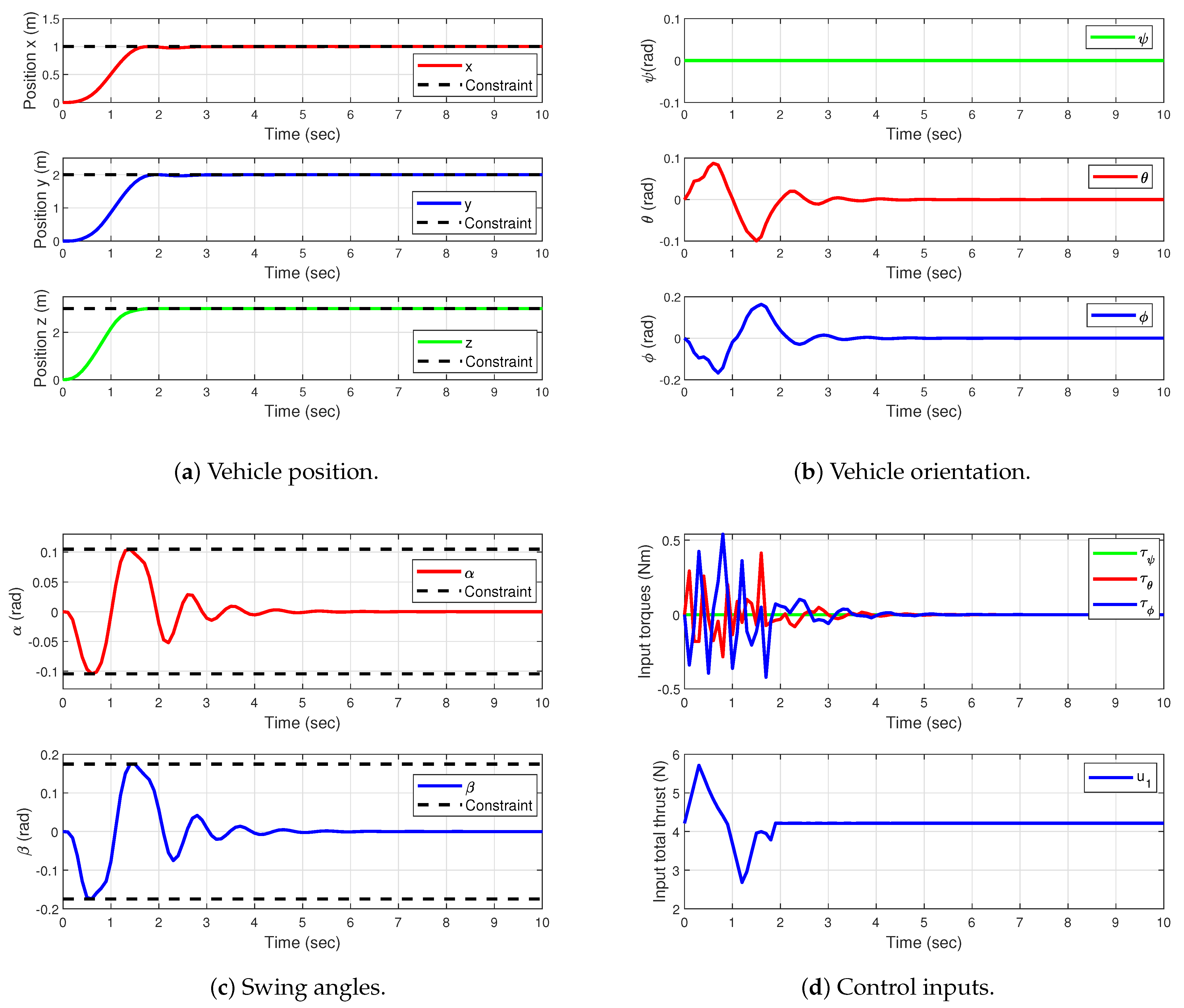
4.1. MPC Performance

In transport operations with multirotors, rapid handling of loads is required, which can be dangerous because the load can generate unwanted oscillations that can vary the flight conditions—the process must be kept within limits. In this particular process, the use of constraints for positions x and y of the vehicle and in the oscillation angles of the load were considered to avoid overshoots that can cause damage to the transported payload and guarantee safety in operations. The results that correspond to the constrained predictive controller are presented in Figure 2.
Figure 2a displays the positions x, y, and z of the quadrotor with their respective constraints 0 x 1 , 0 y 2 , and 0 z 3 . The signals responded quickly to reach the reference in no longer than 3 s. The controller kept each constrained position x and y at its reference value without any overshoots in the transient responses to avoid further oscillations of the load angles.
In Figure 2b the attitude of the quadrotor is shown. No constraint was applied; however, lower values in θ and ϕ angles occurred in comparison to the unconstrained predictive control.
Figure 2c presents the swing angles of the suspended load with their respective constraints, for 0.1047 α 0.1047 and 0.1745 β 0.1745 . As can be seen, the predictive controller kept the oscillation within the established values, demonstrating good performance.
Figure 2d shows the variations of the control inputs in the quadrotor, which ensured that the oscillations of the suspended load did not exceed the values established in the constraints and that the air vehicle could stabilize quickly. In the bottom plot of this figure, we can see the force u 1 in the z axis that stabilized at ( m + M ) g maintain hovering, and in the top plot the control torques τ ψ , τ θ , and τ ϕ .
In summary, numerical simulations have been presented that demonstrate good performance by the predictive controller when considering the constraints to attenuate the oscillations of the suspended load. It is possible to place the quadrotor at a desired position while the oscillations of the load do not exceed the proposed limits. Next, the results of not considering the constraints are shown, for comparative purposes.

4.2. Comparative Results

In Figure 3, a direct comparison of the performance of the proposed MPC algorithm with respect to a nonlinear controller based on the feedback linearization proposed in Equation (16) of [22] has been added. The control law in [22] was chosen because it manages to achieve small swing angles of the payload.
For a better understanding of the figures, know that the subscript “c” means the constrained MPC controller and the subscript “l” the algorithm in [22]. In order to contrast the results with a more aggressive strategy, we also added the unconstrained MPC control law, which is referred to with the subscript “u”. The performance responses of all controllers are displayed in Figure 3. In Figure 3c we can observe the swing angles. It is clear that [22] achieved smaller maximum angles, but the oscillation times for α and β were longer than in the MPC strategy. Moreover, by analyzing Figure 3a, it is possible to appreciate better performance in the vehicle position response of the proposed constrained MPC controller with respect to [22], because the settling time of the vehicle position obtained from control law u l was larger than that obtained with the MPC law. In summary, ref. [22] achieveed small swing angles of the payload but at the cost of poor performance in the vehicle positioning and settling time of the payload swing. In contrast, this proposal produced shorter settling times for the payload and vehicle positioning while still meeting the constraints imposed on the payload swing angles.
In order to quantify the comparisons, Table 3 summarizes the results of the proposed controller and those of the algorithm in [22] with respect to performance measures and oscillation angles. We computed for α and β , the setting time (Ts) and the maximum swing (MS). The superior performance of the proposed scheme over the one in [22] is evidenced by the running-time cost J M P C .

5. Conclusions

This work presents the formulation of a model-based predictive controller meant to solve the problem of transporting a payload suspended by a cable from a multi-rotor-type unmanned aerial vehicle. This strategy considers the three-dimensional translation and rotation of the aerial vehicle, and the payload dynamics. The dynamic model was obtained by formulating a Euler–Lagrange in a global approach that mathematically describes the relationship of the vehicle, the load, and the cable. Next, an affine representation of the input of the model was derived to obtain a linear model for the MPC design. It is worth mentioning that the steps carried out to obtain the linear model of the quadrotor-payload are specific for this system, and the linear model was used as a prediction model for the control strategy. Finally, we evaluated the dynamic model of the UAV with a suspended load, and the proposed controller, using a numerical simulation software. The simulations showed excellent performance by the MPC in comparison to a nonlinear controller based on feedback linearization from the literature. Therefore, the proposed controller demonstrated its ability to precisely control the multi-rotor and achieve rapid attenuation of the oscillation of the suspended load while keeping it within the limits of the constraints. Future work will include considering a flexible cable in the mathematical model and an MPC with variable constraints.

Author Contributions

Conceptualization, G.V.-P. and M.-E.G.-S.; methodology, N.U.-B. and O.H.-G.; software, F.-R.L.-E. and J.A.H.-M.; validation, N.U.-B. and O.H.-G.; writing—original draft preparation, G.V.-P. and M.-E.G.-S.; writing—review and editing, N.U.-B., O.H.-G., F.-R.L.-E. and J.A.H.-M. All authors have read and agreed to the published version of the manuscript.

Funding

This research was funded by Tecnológico Nacional de México grant number 9992.21-P.

Institutional Review Board Statement

Not applicable.

Informed Consent Statement

Not applicable.

Conflicts of Interest

The authors declare no conflict of interest.

Appendix A. Nomenclature

Table A1 and Table A2 show the lists of variables used in the mathematical model and controller derivations.
Table A1. Mathematical model variables.
VariableDescription
O : x O , y O , z O Inertial frame
B : x B , y B , z B Body-fixed frame for quadrotor
ξ : x, y, zQuadrotor linear positions
η : ψ , θ , ϕ Quadrotor angular positions (yaw, pitch, roll)
μ : α , β Oscillations angles of the payload
ξ p : x p , y p , z p Payload position
qGeneralized coordinates vector
rUnit vector of vehicle center of mass to payload
lCable length
dDistance from motors to center of mass
M , m Quadrotor and payload masses
gGravitational acceleration constant
u: u 1 , τ Control inputs
u 1 Total propulsive force
f P i Propulsion force provided by the motor i
τ : τ ψ , τ θ , τ ϕ Input torques
LLagrangian
T Q S P , V q Total kinetic and potential energy
I x , I y , I z Moments of inertia in x, y and z
I p Moment of inertia of the suspended payload
χ State vector
χ e q , u e q Equilibrium state and input vectors
y c Output vector
A c , B c , C c Continuous-time model matrices
Table A2. Predictive control variables.
VariableDescription
A d , B d , C d Discrete-time model matrices
ζ Augmented state
A ζ , B ζ , C ζ Augmented model matrices
x k , u k , y k Discrete state, input and output vectors
Δ u k Increment in control signal
n y , n u Prediction and control horizons
P ζ ζ , P ζ Δ u Augmented state prediction matrices
P y ζ , P y Δ u Output prediction matrices
P x ζ State prediction matrix
P u Δ u , P u , ζ Input prediction matrices
x Column vector of prediction of x
Q , R State and input penalty matrices
y ^ k Independent model output
d ^ Model residual estimate
J M P C Cost function
x * Optimal value of x.
r ^ Setpoint
c o l ( A i ) Block column vector of A i matrices
d i a g ( A i ) Block diagonal matrix of A i matrices
m a x , m i n Maximum and minimum bound of a variable
T s Sampling time
M a , q a ( ζ k ) Constraints matrices

References

  1. Bernard, M.; Kondak, K. Generic slung load transportation system using small size helicopters. In Proceedings of the 2009 IEEE International Conference on Robotics and Automation, Kobe, Japan, 12–17 May 2009; pp. 3258–3264. [Google Scholar]
  2. Ghadiok, V.; Goldin, J.; Ren, W. Autonomous indoor aerial gripping using a quadrotor. In Proceedings of the 2011 IEEE/RSJ International Conference on Intelligent Robots and Systems, San Francisco, CA, USA, 25–30 September 2011; pp. 4645–4651. [Google Scholar]
  3. Mellinger, D.; Lindsey, Q.; Shomin, M.; Kumar, V. Design, modeling, estimation and control for aerial grasping and manipulation. In Proceedings of the 2011 IEEE/RSJ International Conference on Intelligent Robots and Systems, San Francisco, CA, USA, 25–30 September 2011; pp. 2668–2673. [Google Scholar]
  4. Baizid, K.; Giglio, G.; Pierri, F.; Trujillo, M.A.; Antonelli, G.; Caccavale, F.; Viguria, A.; Chiaverini, S.; Ollero, A. Experiments on behavioral coordinated control of an unmanned aerial vehicle manipulator system. In Proceedings of the 2015 IEEE International Conference on Robotics and Automation (ICRA), Seattle, WA, USA, 26–30 May 2015; pp. 4680–4685. [Google Scholar]
  5. Cruz, P.J.; Oishi, M.; Fierro, R. Lift of a cable-suspended load by a quadrotor: A hybrid system approach. In Proceedings of the 2015 American Control Conference (ACC), Chicago, IL, USA, 1–3 July 2015; pp. 1887–1892. [Google Scholar]
  6. Pounds, P.E.; Bersak, D.R.; Dollar, A.M. Stability of small-scale UAV helicopters and quadrotors with added payload mass under PID control. Auton. Robot. 2012, 33, 129–142. [Google Scholar] [CrossRef]
  7. Palunko, I.; Cruz, P.; Fierro, R. Agile load transportation: Safe and efficient load manipulation with aerial robots. IEEE Robot. Autom. Mag. 2012, 19, 69–79. [Google Scholar] [CrossRef]
  8. Guerrero-Sánchez, M.E.; Mercado-Ravell, D.A.; Lozano, R.; García-Beltrán, C.D. Swing-attenuation for a quadrotor transporting a cable-suspended payload. ISA Trans. 2017, 68, 433–449. [Google Scholar] [CrossRef] [PubMed]
  9. Klausen, K.; Fossen, T.I.; Johansen, T.A. Nonlinear control with swing damping of a multirotor UAV with suspended load. J. Intell. Robot. Syst. 2017, 88, 379–394. [Google Scholar] [CrossRef]
  10. Guerrero-Sánchez, M.E.; Hernández-González, O.; Lozano, R.; García-Beltrán, C.D.; Valencia-Palomo, G.; López-Estrada, F.R. Energy-Based Control and LMI-Based Control for a Quadrotor Transporting a Payload. Mathematics 2019, 7, 1090. [Google Scholar] [CrossRef] [Green Version]
  11. Guerrero-Sánchez, M.; Lozano, R.; Castillo, P.; Hernández-González, O.; García-Beltrán, C.; Valencia-Palomo, G. Nonlinear control strategies for a UAV carrying a load with swing attenuation. Appl. Math. Model. 2021, 91, 709–722. [Google Scholar] [CrossRef]
  12. Liang, X.; Lin, H.; Zhang, P.; Wu, S.; Sun, N.; Fang, Y. A Nonlinear Control Approach for Aerial Transportation Systems with Improved Antiswing and Positioning Performance. IEEE Trans. Autom. Sci. Eng. 2020. [Google Scholar] [CrossRef]
  13. Ren, Z.; Hu, C.; Wu, H.; Sun, B.; Guo, Y. Obstacle Avoidance-based Control System Design of UAV with Suspended Payload. In Proceedings of the 2020 39th Chinese Control Conference (CCC), Shenyang, China, 27–29 July 2020; pp. 6839–6844. [Google Scholar]
  14. Pizetta, I.H.B.; Brandão, A.S.; Sarcinelli-Filho, M. Load Transportation by Quadrotors in Crowded Workspaces. IEEE Access 2020, 8, 223941–223951. [Google Scholar] [CrossRef]
  15. Pratama, G.N.P.; Masngut, I.; Cahyadi, A.I.; Herdjunanto, S. Robustness of PD control for transporting quadrotor with payload uncertainties. In Proceedings of the 2017 3rd International Conference on Science and Technology-Computer (ICST), Yogyakarta, Indonesia, 11–12 July 2017; pp. 11–15. [Google Scholar]
  16. Rezaei Lori, A.A.; Danesh, M.; Amiri, P.; Ashkoofaraz, S.Y.; Azargoon, M.A. Transportation of an Unknown Cable-Suspended Payload by a Quadrotor in Windy Environment under Aerodynamics Effects. In Proceedings of the 2021 7th International Conference on Control, Instrumentation and Automation (ICCIA), Tabriz, Iran, 23–24 February 2021; pp. 1–6. [Google Scholar]
  17. Lv, Z.; Li, S.; Wu, Y.; Wang, Q.G. Adaptive Control for a Quadrotor Transporting a Cable-suspended Payload with Unknown Mass in the Presence of Rotor Downwash. IEEE Trans. Veh. Technol. 2021. [Google Scholar] [CrossRef]
  18. Alothman, Y.; Gu, D. Quadrotor transporting cable-suspended load using iterative Linear Quadratic regulator (iLQR) optimal control. In Proceedings of the 2016 8th Computer Science and Electronic Engineering (CEEC), Colchester, UK, 28–30 September 2016; pp. 168–173. [Google Scholar]
  19. Sun, B.; Chaofang, H.; Cao, L.; Wang, N.; Zhou, Y. Trajectory Planning of Quadrotor UAV with Suspended Payload Based on Predictive Control. In Proceedings of the 2018 37th Chinese Control Conference (CCC), Wuhan, China, 25–27 July 2018; pp. 10049–10054. [Google Scholar]
  20. Erasmus, A.; Jordaan, H. Linear Quadratic Gaussian Control of a Quadrotor with an Unknown Suspended Payload. In Proceedings of the 2020 International SAUPEC/RobMech/PRASA Conference, Cape Town, South Africa, 29–31 January 2020; pp. 1–6. [Google Scholar]
  21. Wang, Y.; Cai, H.; Zhang, J.; Li, X. Disturbance Attenuation Predictive Optimal Control for Quad-Rotor Transporting Unknown Varying Payload. IEEE Access 2020, 8, 44671–44686. [Google Scholar] [CrossRef]
  22. Pizetta, I.H.B.; Brandão, A.S.; Sarcinelli-Filho, M. Modelling and control of a PVTOL quadrotor carrying a suspended load. In Proceedings of the 2015 International Conference on Unmanned Aircraft Systems (ICUAS), Denver, CO, USA, 9–12 June 2015; pp. 444–450. [Google Scholar]
  23. Valencia-Palomo, G.; Rossiter, J.A. Auto-tuned predictive control based on minimal plant information. IFAC Proc. Vol. 2009, 42, 554–559. [Google Scholar] [CrossRef]
  24. Rossiter, J. A First Course in Predictive Control; CRC Press: Boca Raton, FL, USA, 2018. [Google Scholar]
  25. Garriga, J.L.; Soroush, M. Model predictive control tuning methods: A review. Ind. Eng. Chem. Res. 2010, 49, 3505–3515. [Google Scholar] [CrossRef]
  26. Gutiérrez-Urquídez, R.; Valencia-Palomo, G.; Rodríguez-Elias, O.M.; Trujillo, L. Systematic selection of tuning parameters for efficient predictive controllers using a multiobjective evolutionary algorithm. Appl. Soft Comput. 2015, 31, 326–338. [Google Scholar] [CrossRef]
Figure 1. Three-dimensional quadrotor with a cable-suspended payload.
Mathematics 09 01822 g001
Figure 2. Results for the proposed predictive controller.
Mathematics 09 01822 g002
Figure 3. Comparison results for the proposed MPC with the controller of [22].
Mathematics 09 01822 g003
Table 1. System parameters.
ParameterValueUnits
M 0.4 m
m 0.03 m
d 0.1 m
l 0.35 m
g 9.8 m/s 2
I x 1.77 × 10 3 kgm 2
I y 1.77 × 10 3 kgm 2
I z 3.54 × 10 3 kgm 2
I p 1.00 × 10 6 kgm 2
Table 2. Controller parameters.
ParameterValueUnits
T s 0.1 s
n y 10
n u 3
QI
R 0.00001 × I
Table 3. Performances of the proposed control and the controller in [22].
ControllerCost J MPC Swing AngleTs (s)MS (Rad)
u c 624.8 α 3.50.1
β 3.50.175
u u 985.1 α 3.50.28
β 3.50.5
u l 1997.3 α 7.20.05
β 7.20.15
Publisher’s Note: MDPI stays neutral with regard to jurisdictional claims in published maps and institutional affiliations.

