Three-Dimensional Numerical Study of the Effect of Protective Barrier on the Dispersion of the Contaminant in a Building

Abstract

The finite volume method and potential-vorticity vector formalism in their three-dimensional form were used to numerically study the impact of an adiabatic and impermeable vertical barrier on the dispersion of a local aero-contaminant due to the double-diffusive Rayleigh–Benard convection inside a cubic container. Different governing parameters such as the Rayleigh number, buoyancy ratio and barrier height were analyzed for Le = 1.2 and Pr = 0.7, representing an air-contaminant mixture. The potential-vector-vorticity formalism in the three-dimensional form allowed the elimination of the pressure terms appearing in the Navier–Stokes equations. It was found that the heat and mass transfer as well as the effectiveness of the barrier in reducing contaminant dispersion are strongly influenced by the buoyancy ratio, the barrier size and the Rayleigh number. In addition, the barrier effectiveness is more than 70% for a height of half the building height.

1. Introduction

Improving air quality has been one of the most important objectives of scientific research in recent years, particularly in view of the spread of viruses. The assessment of air quality is based on the measurement and identification of all types of air pollutants, without attempting to distinguish between pollutants of natural origin and those resulting from human activity or virus circulation. An air monitoring system or solution can be used to manage exposure to air pollutants when the source strength is local and moderate, such as smoke, dust or sprays. Several researchers have investigated air quality monitoring using analytical, experimental and numerical models.

Many dangerous chemical pollutants are present in the indoor environment that adversely affect people’s comfort and health [1]. Formaldehyde and volatile organic compounds (VOCs) are the main pollutants emitted from building materials that humans may be exposed to through inhalation [2,3]. Several authors have investigated the emission characteristics of formaldehyde and volatile organic compounds from building materials and the associated health risks in order to achieve an effective source control and create a sustainable built environment. The researchers focused on creating analytical or numerical solutions to predict the concentration of pollutants in a room or indoor environment based on the mass transfer analysis [4,5,6,7,8]. Wiglusz et al. [9] examined an experimental study of the effect of temperatures on emissions of formaldehyde and volatile organic compounds (VOCs) from relevant plates. They showed that at 23 and 29 °C, there are no formaldehyde emissions and they observed very low emissions of VOCs. But at 50 °C, the authors noticed high initial emissions of formaldehyde and VOCs, which decreased over time. Xiong et al. [10] theoretically studied the overall effect of temperature and relative humidity on the emission rate of pollutants from building materials. In addition, the authors proposed a new approach to assess the impact on human health due to pollutants emitted at varying temperatures and relative humidity and concluded that there is a correlation between the likelihood of human cancer (HCP) and environmental factors. Deng et al. [11] numerically examined the double diffusive mixed convection in a bidimensional cavity with contaminant. They noticed that the flow structure due to a double-diffusive convection can detect indoor airflow, heat transfer structures and pollutants. Yu-Shu et al. [12] numerically studied the forced and mixed convection in a cavity filled with a porous medium with a local contaminant source. They found a critical factor in terms of the Reynolds number and Darcy number for a flow structure transition from vortex-free to multi-vortexes. Zhao et al. [13] numerically studied the double diffusive convection in the cavity saturated by porous media with local heat and a contaminant source. The authors concluded that the permeability of porous medium strongly affects the heat and mass transfer in the cavity. A numerical investigation of double diffusive convection in the enclosure with local CO₂ source was studied by Arellano et al. [14]. The authors noted that the Nusselt number is directly affected by the location of the contaminant’s source. Li et al. [15] numerically studied the double diffusive convection and radiation effect on the dispersion of gas contaminant in a cavity. They noticed that surface radiation represents about 37–71% of the heat transfer from the heat sources. They also remarked that the diffusion of the contaminants is dependent on the temperature. Consequently, the contaminants exhibit different distribution patterns in the air.

Several numerical and mathematical methods have been used in recent years to solve the convection-diffusion differential equation. Abolhasani et al. [16] introduced a resolution method based on the variational iteration method (VIM). Geiser et al. [17] applied parallel iterative splitting methods, allowing an acceleration of the solver and subsequently a reduction of the computation time.

Emissions and dispersion of viruses or other volatile organic compounds (VOCs) inside buildings is a major problem that has needed to be addressed in recent years. This is because airflow near walls and under the influence of thermal gradient plays an important role in the transport of pollutants from the emitting source to the ambient air and because recirculating air in forced convection can be dangerous in terms of increasing the dispersion of pollutants. Therefore, for these reasons, an effective prediction of the manner in which contaminants are emitted and dispersed in natural convection allows us to control their hazards.

The main objective of this work is to analyze the flow pattern of the natural 3D double-diffusive convection in an air-filled building with a local source of contaminants, using the finite volume method and the vector potential-vorticity formalism in three-dimensional form, to analyze the mode of dispersion of the contaminants, and to examine the efficiency of the placement of a barrier to avoid contamination of the whole building volume for different Rayleigh numbers and buoyancy ratios.

2. Physical Configuration and Governing Equations

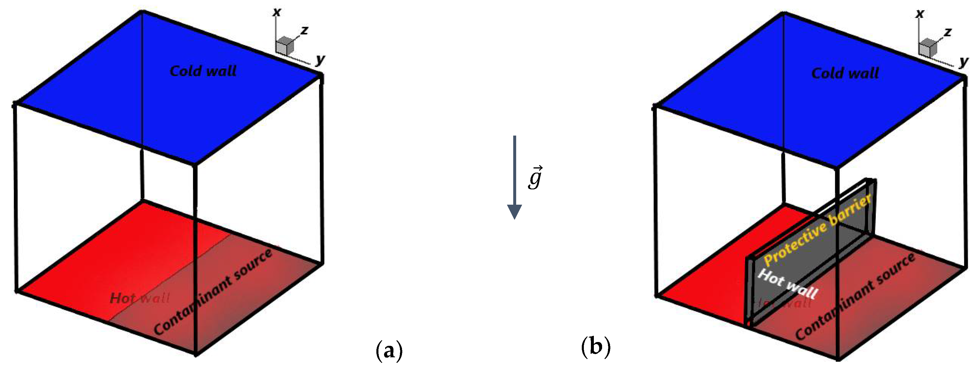
In this section, the physical configuration, the assumptions and the governing equations are described. The studied configuration, illustrated in Figure 1, represents an air-filled cavity with a local source of contamination located at the bottom surface. The air-contaminant mixture in the cavity is characterized by the Lewis and Prandtl numbers Le = 1.2 and Pr = 0.72, respectively. The bottom wall is hot (T′_H) and the top wall is cold (T′_c). However, the source of contamination is located in half of the surface of the bottom wall with a high concentration (C′_h). The other half of the bottom wall and the top wall have a zero concentration (C′_l). The remaining walls (vertical lateral sides) are considered adiabatic, impermeable. The cavity is a cubic of width L. The impact of the insertion of an adiabatic, impermeable vertical barrier, positioned in the middle of the bottom wall, on the dispersion of the contaminant in the whole cavity was investigated. The effect of the height (H’) of this wall as well as the ratio of the volume forces (N) and the Rayleigh number (Ra) were studied, while the thickness of the barrier was fixed at 0.05 × L.

In this study, the following assumptions were adopted to simplify the formulation of the mathematical model:

• The fluid in the cavity is assumed to be Newtonian and incompressible.
• The flow is assumed to be laminar.
• Heat transfer by radiation is negligible.
• There is no heat or mass source and no chemical reaction
• Soret and Dufour effects are negligible
• The thermo-physical properties of the fluid are assumed to be constant and the Boussinesq approximation is adopted.

The last approximation assumes that the density is constant in all terms of the transfer equations except in the gravitational term, where it varies linearly with temperature and concentration by the following relation:

$$\rho ={\rho }_0\left[1-{\beta }_T\left(T^{\prime }-T_0\right)-{\beta }_C\left(C^{\prime }-C_0\right)\right]$$

(1)

where $T^{\prime }$ is the temperature of the fluid mixture and $C^{\prime }$ is the concentration of the contaminant at a given point in the cavity. ${\rho }_0$, $T_0$ and $C_0$ are respectively the reference density, temperature and concentration. ${\beta }_T$ and ${\beta }_C$ represent the thermal and solutal expansion coefficients of the fluid. They are defined by:

$${\beta }_T=-\frac{1}{{\rho }_0}{\left(\frac{\partial \rho }{\partial T^{\prime }}\right)}_{P^{\prime },C^{\prime }}\mathrm{and}{\beta }_C=-\frac{1}{{\rho }_0}{\left(\frac{\partial \rho }{\partial C^{\prime }}\right)}_{P^{\prime },T^{\prime }}.$$

(2)

The fluid motion in the cavity is induced by density variations due to temperature and concentration gradients. Considering the simplifying assumptions, the general equations governing the fluid flow in double diffusion convection are, respectively, the continuity equation, the conservation of momentum, the conservation of energy and the conservation of mass, which can be written in the following vector form:

$$\mathrm{Continuity}\nabla \overrightarrow{V}{}^{\prime }=0$$

(3)

$$\mathrm{Momentum}\frac{\partial {\overrightarrow{V}}^{\prime }}{\partial t^{\prime }}+\left(\overrightarrow{V}\times {}^{\prime }\overrightarrow{\nabla }\right){\overrightarrow{V}}^{\prime }=-\frac{1}{{\rho }_0}\overrightarrow{\nabla }{P}^{\prime }+\nu \Delta {\overrightarrow{V}}^{\prime }+\left[1-{\beta }_T\left(T^{\prime }-T_0\right)-{\beta }_C\left(C^{\prime }-C_0\right)\right]\overrightarrow{g}$$

(4)

$$\mathrm{Energy}\frac{\partial T^{\prime }}{\partial t^{\prime }}+{\overrightarrow{V}}^{\prime }\times \nabla T^{\prime }=\alpha \Delta T^{\prime }$$

(5)

$$\mathrm{Mass}\frac{\partial C^{\prime }}{\partial t^{\prime }}+{\overrightarrow{V}}^{\prime }\times \nabla C^{\prime }=D\Delta C^{\prime }.$$

(6)

3. Resolution Method Based on the Vorticity-Potential Vector Formalism and Non-Dimensioning of Equations

To solve the Navier–Stokes equations, vector potential-vorticity formalism is used, which in a three-dimensional configuration eliminates the pressure term from the momentum equation. This method of resolution was adopted by Mallinson and de Vahl Davis [18] and Wakashima and Saitoh [19]. The vector potential and vorticity are defined by the following two relations, respectively:

$${\overrightarrow{\omega }}^{\prime }=\overrightarrow{\nabla }\times {\overrightarrow{V}}^{\prime }\mathrm{and}{\overrightarrow{V}}^{\prime }=\overrightarrow{\nabla }\times {\overrightarrow{\psi }}^{\prime }.$$

(7)

The dimensionless formulation of the problem is performed by defining a dimensionless space variable, dimensionless time, dimensionless velocity, vector potential, vorticity, dimensionless temperature and concentration as:

$$\begin{array}{cc}X=x/LY=y/L& Z=z/LH=H^{\prime }/L\\ \omega =\alpha {\omega }^{\prime }/L^{2}t=\alpha t^{\prime }/L^2& V=L{V}^{\prime }/\alpha \psi ={\psi }^{\prime }/\alpha \\ T=\frac{T^{\prime }-{T^{\prime }}_c}{{T^{\prime }}_H-{T^{\prime }}_c}& C=\frac{C^{\prime }-{C^{\prime }}_l}{{C^{\prime }}_h-{C^{\prime }}_l}.\end{array}$$

(8)

After using the dimensionless variables, the system of equations governing the problem becomes:

$$\frac{\partial V_x}{\partial X}+\frac{\partial V_y}{\partial Y}+\frac{\partial V_z}{\partial Z}=0$$

(9)

$$-\overrightarrow{\omega }={\nabla }^2\overrightarrow{\psi }$$

(10)

$$\frac{\partial \overrightarrow{\omega }}{\partial t}+\left(\overrightarrow{V}\times \overrightarrow{\nabla }\right)\overrightarrow{\omega }-\left(\overrightarrow{\omega }\times \overrightarrow{\nabla }\right)\overrightarrow{V}=Pr\times {\nabla }^2\overrightarrow{\omega }+RaPr\left[\frac{\partial T}{\partial z},0,-\frac{\partial T}{\partial x}\right]-RaPrN\left[\frac{\partial C}{\partial z},0,-\frac{\partial C}{\partial x}\right]$$

(11)

$$\frac{\partial T}{\partial t}+\overrightarrow{V}\times \nabla T={\nabla }^{2}T$$

(12)

$$\frac{\partial C}{\partial t}+\overrightarrow{V}\times \overrightarrow{\nabla }C=\frac{1}{Le}{\overrightarrow{\nabla }}^{2}C.$$

(13)

The dimensionless parameters appearing in the equations are:

$$N=\frac{{\beta }_C\left({C^{\prime }}_h-{C^{\prime }}_l\right)}{{\beta }_T\left({T^{\prime }}_H-{T^{\prime }}_c\right)}Ra=\frac{g{\beta }_T\left({T^{\prime }}_h-{T^{\prime }}_c\right)L^3}{\nu \alpha }Pr=\frac{\nu }{\alpha }Le=\frac{\alpha }{D}.$$

(14)

N represents the ratio of the solutal volume forces to the thermal volume forces, also called the buoyancy ratio. Ra, Pr and Le represent the thermal Rayleigh number, Prandtl number and Lewis number, respectively.

The local Nusselt and Sherwood numbers are written as follows:

$$Nu={\frac{\partial T}{\partial x}|}_{x=0,1}Sh={\frac{\partial C}{\partial x}|}_{x=0,1}.$$

(15)

The average Nusselt and Sherwood numbers on the walls are:

$$\overline{N}u={{\displaystyle \int }}_0^1{{\displaystyle \int }}_0^{1}Nu\times \partial y\partial z\overline{S}h={{\displaystyle \int }}_0^1{{\displaystyle \int }}_0^{1}Sh\times \partial y\partial z.$$

(16)

The boundary conditions are as follows:

$$\mathrm{Temperature}:T=1\mathrm{at}X=0,T=0\mathrm{at}x=1,\frac{\partial T}{\partial n}=0\mathrm{on}\mathrm{the}\mathrm{remaining}\mathrm{walls}(\mathrm{adiabatic})$$

(17)

$$\mathrm{Concentration}:C=1\mathrm{at}X=0,Y>0.5,C=0\mathrm{at}X=1\mathrm{and}X=0,Y<0.5,\frac{\partial C}{\partial n}=0\mathrm{on}\mathrm{the}\mathrm{other}\mathrm{walls}(\mathrm{impermeable})$$

(18)

$$\mathrm{Vorticity}:\begin{array}{c}{\omega }_x=0,{\omega }_y=-\frac{\partial V_z}{\partial X},{\omega }_z=\frac{\partial V_y}{\partial X}\mathrm{at}X=0\mathrm{and}1\\ {\omega }_x=\frac{\partial V_z}{\partial Y},{\omega }_y=0,{\omega }_z=-\frac{\partial V_x}{\partial Y}\mathrm{at}Y=0\mathrm{and}1\\ {\omega }_x=-\frac{\partial V_y}{\partial Z},{\omega }_y=\frac{\partial V_x}{\partial Z},{\omega }_z=0\mathrm{at}Z=0\mathrm{and}1\end{array}$$

(19)

$$\mathrm{Vector\; potential}:\begin{array}{c}\frac{\partial {\psi }_x}{\partial X}={\psi }_y={\psi }_z=0\mathrm{at}X=0\mathrm{and}1\\ {\psi }_x=\frac{\partial {\psi }_y}{\partial Y}={\psi }_z=0\mathrm{at}Y=0\mathrm{and}1\\ {\psi }_x={\psi }_y=\frac{\partial {\psi }_z}{\partial Z}=0\mathrm{at}Z=0\mathrm{and}1\end{array}$$

(20)

$$\mathrm{Velocity}:V_x=V_y=V_z=0\mathrm{On}\mathrm{all}\mathrm{walls}.$$

(21)

The boundary conditions of the adiabatic and impermeable barrier are:

$$V_x=V_y=V_z=0,\frac{\partial T}{\partial n}=0,\frac{\partial C}{\partial n}=0.$$

(22)

4. Numerical Modeling, Discretization, Grid Sensitivity Study and Code Verification

4.1. Finite Volume Method

The numerical code developed during this work was based on the finite volume method. This method consists of subdividing the three-dimensional computational domain into a number of control volumes [20]. The dependent variable considered is calculated at each of these points. The algebraic equations defined at these nodes are obtained by integrating the conservation equations through the control volumes for each node.

4.2. Meshing

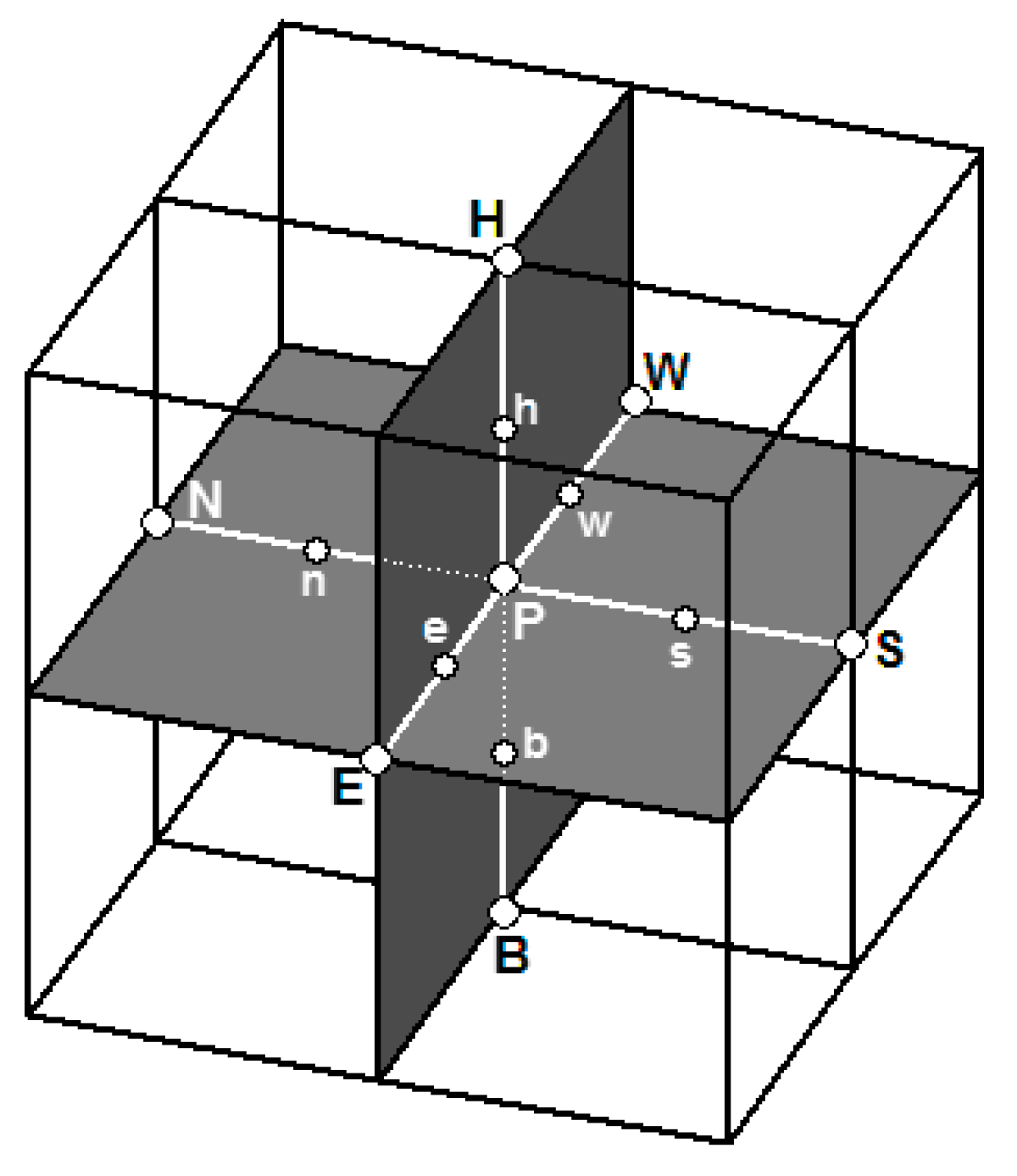
As shown in Figure 2, a rectangular mesh was considered with Nx nodes on the (x) axis, Ny nodes on the (y) axis and Nz nodes on the (z) axis.

The discrete variables t, x and y are written as follows:

• i: node index on the (x) axis
• j: node index on the (y) axis
• k: node index on the (z) axis

$$x_1=0,x_2=0+\frac{\Delta x}{2},i=3,Nx-1,x_i=0+\left(i-1\right)\Delta x\mathrm{and}{x}_{Nx}=1$$

(23)

$$y_1=0,y_2=0+\frac{\Delta y}{2},j=3,Ny-1,y_j=0+\left(j-1\right)\Delta y\mathrm{and}{y}_{Ny}=1$$

(24)

$$z_1=0,z_2=0+\frac{\Delta z}{2},k=3,Nz-1,z_k=0+\left(k-1\right)\Delta z\mathrm{and}{z}_{Nz}=1$$

(25)

• Δx is the space step size on the (x) axis
• Δy is the space step size on the (y) axis
• Δz is the space step size on the (z) axis
• And Δt is the time step

Δx, Δy and Δz were defined by the following relations:

$$\Delta x=\frac{1}{Nx-1},\Delta y=\frac{1}{Ny-1}\mathrm{and}\Delta z=\frac{1}{Nz-1}.$$

(26)

4.3. Equations Discretization

The transfer Equations (11)–(13) can be written in the following general form:

$$\frac{\partial \mathrm{\Phi }}{\partial t}+\frac{\partial }{\partial x}\left(V_x·\mathrm{\Phi }-{\mathrm{\Gamma }}_{\mathrm{\Phi }}\frac{\partial \mathrm{\Phi }}{\partial x}\right)+\frac{\partial }{\partial y}\left(V_y·\mathrm{\Phi }-{\mathrm{\Gamma }}_{\mathrm{\Phi }}\frac{\partial \mathrm{\Phi }}{\partial y}\right)+\frac{\partial }{\partial z}\left(V_z·\mathrm{\Phi }-{\mathrm{\Gamma }}_{\mathrm{\Phi }}\frac{\partial \mathrm{\Phi }}{\partial z}\right)=S_{\mathrm{\Phi }}$$

(27)

with $\mathrm{\Phi }$: T, C, ${\omega }_x$, ${\omega }_y$ or ${\omega }_z$, ${\mathrm{\Gamma }}_{\mathrm{\Phi }}$: dimensionless coefficient and $S_{\mathrm{\Phi }}$: source term.

Table 1. Overview of the dimensionless equations.

$\Phi$	${\Gamma }_{\Phi }$	$S_{\Phi }$
${\omega }_x$	Pr	${\omega }_x\frac{\partial V_x}{\partial X}+{\omega }_y\frac{\partial V_x}{\partial Y}+{\omega }_z\frac{\partial V_x}{\partial Z}+RaPr\frac{\partial T}{\partial Z}$
${\omega }_y$	Pr	${\omega }_x\frac{\partial V_y}{\partial X}+{\omega }_y\frac{\partial V_y}{\partial Y}+{\omega }_z\frac{\partial V_y}{\partial Z}$
${\omega }_z$	Pr	${\omega }_x\frac{\partial V_z}{\partial X}+{\omega }_y\frac{\partial V_z}{\partial Y}+{\omega }_z\frac{\partial V_z}{\partial Z}-RaPr\frac{\partial T}{\partial Z}$
T	1	0
C	$\frac{1}{Le}$	0

summarizes all the transfer equations, momentum, energy and mass.

Equation (27) can be written as:

$$\frac{\partial \mathrm{\Phi }}{\partial t}+\frac{\partial L_x}{\partial X}+\frac{\partial L_y}{\partial Y}+\frac{\partial L_z}{\partial Z}=S_{\mathrm{\Phi }}$$

(28)

where $L_x,L_y\mathrm{and}{L}_z$ are the total convection and diffusion fluxes in the x, y and z directions, respectively, and are defined by:

$$L_x=V_x\mathrm{\Phi }-{\mathrm{\Gamma }}_{\mathrm{\Phi }}\frac{\partial \mathrm{\Phi }}{\partial X},L_y=V_y\mathrm{\Phi }-{\mathrm{\Gamma }}_{\mathrm{\Phi }}\frac{\partial \mathrm{\Phi }}{\partial Y}\mathrm{and}{L}_z=V_z\mathrm{\Phi }-{\mathrm{\Gamma }}_{\mathrm{\Phi }}\frac{\partial \mathrm{\Phi }}{\partial Z}.$$

(29)

The integration of Equation (27) on a control volume gives (Patankar [21]):

$$\left({\mathrm{\Phi }}_p-{\mathrm{\Phi }}_p^{°}\right)\Delta x\Delta y\Delta z+\left(L_{xe}-L_{xw}\right)\Delta y\Delta z\Delta t+\left(L_{yn}-L_{ys}\right)\Delta x\Delta z\Delta t+\left(L_{zh}-L_{zb}\right)\Delta x\Delta y\Delta t=\overline{S}\Delta x\Delta y\Delta z\Delta t.$$

(30)

The superscript ° indicates that it is the previous time (according to the explicit scheme).

Equation (29) can be written as:

$$\left({\mathrm{\Phi }}_p-{\mathrm{\Phi }}_p^{°}\right)\frac{\Delta x\Delta y\Delta z}{\Delta t}+\left(L_e-L_w\right)+\left(L_n-L_s\right)+\left(L_h-L_b\right)=\overline{S}\Delta x\Delta y\Delta z$$

(31)

where:

$$L_e=L_{xe}\Delta y\Delta z,L_w=L_{xw}\Delta y\Delta z,L_n=L_{yn}\Delta x\Delta z,L_s=L_{ys}\Delta x\Delta z,L_h=L_{zh}\Delta x\Delta y\mathrm{and}{L}_b=L_{zb}\Delta x\Delta y.$$

(32)

The source term $\overline{S}$ is linearized as:

$$\overline{S}=S_c+S_p{\mathrm{\Phi }}_p$$

(33)

Notably, $S_p$ must be negative to provide stability for numerical simulations.

Integrating the continuity of Equation (9) written in a dimensionless form on to the same control volume, we obtained:

$$\left(V_{xe}\Delta y\Delta z-V_{xw}\Delta y\Delta z\right)+\left(V_{yn}\Delta x\Delta z-V_{ys}\Delta x\Delta z\right)+\left(V_{zh}\Delta x\Delta y-V_{zb}\Delta x\Delta y\right)=0.$$

(34)

We considered:

$$F_e=V_{xe}\Delta y\Delta z\mathrm{and}{F}_w=V_{xw}\Delta y\Delta z;F_n=V_{yn}\Delta x\Delta z\mathrm{and}{F}_s=V_{ys}\Delta x\Delta z;F_h=V_{zs}\Delta x\Delta y\mathrm{and}{F}_b=V_{zb}\Delta x\Delta y$$

(35)

Equation (34) becomes:

$$\left(F_e-F_w\right)+\left(F_n-F_s\right)+\left(F_h-F_b\right)=0$$

(36)

where $F_e,F_w,F_n,F_s,F_h$ and $F_b$ represent the mass flow rates through the faces of the control volume.

Multiplying the discretized continuity Equation (36) by ${\mathrm{\Phi }}_p$ and subtracting it from the general discretized Equation (31) then gives:

$$\begin{array}{c}{\mathrm{\Phi }}_p\left(\frac{\Delta x\Delta y\Delta z}{\Delta t}-S_p\Delta x\Delta y\Delta z\right)+\left(L_e-F_e{\mathrm{\Phi }}_p\right)-\left(L_w-F_w{\mathrm{\Phi }}_p\right)+\left(L_n-F_n{\mathrm{\Phi }}_p\right)-\left(L_s-F_s{\mathrm{\Phi }}_p\right)+\left(L_h-F_h{\mathrm{\Phi }}_p\right)\\ -\left(L_b-F_b{\mathrm{\Phi }}_p\right)=\left(S_c\Delta x\Delta y\Delta z+{\mathrm{\Phi }}_p^{°}\frac{\Delta x\Delta y\Delta z}{\Delta t}\right).\end{array}$$

(37)

We considered the following expressions [21]:

$$\begin{array}{c}\left(L_n-F_n{\mathrm{\Phi }}_p\right)=a_N\left({\mathrm{\Phi }}_p-{\mathrm{\Phi }}_N\right),\left(L_s-F_s{\mathrm{\Phi }}_p\right)=a_S\left({\mathrm{\Phi }}_S-{\mathrm{\Phi }}_p\right),\left(L_e-F_e{\mathrm{\Phi }}_p\right)=a_E\left({\mathrm{\Phi }}_p-{\mathrm{\Phi }}_E\right),\\ \left(L_w-F_w{\mathrm{\Phi }}_p\right)=a_W\left({\mathrm{\Phi }}_W-{\mathrm{\Phi }}_p\right),\left(L_h-F_h{\mathrm{\Phi }}_p\right)=a_H\left({\mathrm{\Phi }}_p-{\mathrm{\Phi }}_H\right),\left(L_b-F_b{\mathrm{\Phi }}_p\right)=a_B\left({\mathrm{\Phi }}_B-{\mathrm{\Phi }}_p\right).\end{array}$$

(38)

Equation (37) becomes:

$$a_p{\mathrm{\Phi }}_p=a_E{\mathrm{\Phi }}_E+a_W{\mathrm{\Phi }}_W+a_N{\mathrm{\Phi }}_N+a_S{\mathrm{\Phi }}_S+a_H{\mathrm{\Phi }}_H+a_B{\mathrm{\Phi }}_B+b_p$$

(39)

where:

$$a_p=a_E+a_W+a_N+a_S+a_H+a_B+\frac{\Delta x\Delta y\Delta z}{\Delta t}-S_p\Delta x\Delta y\Delta z\mathrm{and}{b}_p=S_c\Delta x\Delta y\Delta z+{\mathrm{\Phi }}_p^{°}\frac{\Delta x\Delta y\Delta z}{\Delta t}.$$

(40)

By substituting the function ${\mathrm{\Phi }}_p$ with the temperature T in the general discretized Equation (39), we obtained the discretized energy equation:

$$a_p{T}_p=a_E{T}_E+a_W{T}_W+a_N{T}_N+a_S{T}_S+a_H{T}_H+a_B{T}_B+b_p\mathrm{with}{b}_p=T_p^{°}\frac{\Delta x\Delta y\Delta z}{\Delta t}$$

(41)

By substituting the function ${\mathrm{\Phi }}_p$ with the concentration C in the general discretized Equation (39), we obtained the discretized mass equation:

$$a_p{C}_p=a_E{C}_E+a_W{C}_W+a_N{C}_N+a_S{C}_S+a_H{C}_H+a_B{C}_B+b_p\mathrm{with}{b}_p=C_p^{°}\frac{\Delta x\Delta y\Delta z}{\Delta t}.$$

(42)

To develop the vorticity equation, we replaced the function ${\mathrm{\Phi }}_p$ for each component ${\omega }_x,{\omega }_y\mathrm{and}{\omega }_z$, respectively, and obtained the following equations:

• According to x-direction, ${\mathrm{\Phi }}_p={\omega }_x$:

  $$a_p{\omega }_{xp}=a_E{\omega }_{xE}+a_W{\omega }_{xW}+a_N{\omega }_{xN}+a_S{\omega }_{xS}+a_H{\omega }_{xH}+a_B{\omega }_{xB}+b_p$$

  (43)

  with

  $$\begin{array}{c}{b}_p={\omega }_{xp}^{°}\frac{\Delta x\Delta y\Delta z}{\Delta t}+{\omega }_{xp}\left(\frac{V_{xE}-V_{xw}}{2}\right)\Delta y\Delta z+{\omega }_{yp}\left(\frac{V_{xS}-V_{xN}}{2}\right)\Delta x\Delta z+{\omega }_{zp}\left(\frac{V_{xH}-V_{xB}}{2}\right)\Delta x\Delta y\\ +RaPr\left(\frac{T_H-T_B}{2}\right)\Delta x\Delta y-RaPrN\left(\frac{C_H-C_B}{2}\right)\Delta x\Delta y.\end{array}$$

  (44)
• According to y-direction, ${\mathrm{\Phi }}_p={\omega }_y$:

  $$a_p{\omega }_{xp}=a_E{\omega }_{yE}+a_W{\omega }_{yW}+a_N{\omega }_{yN}+a_S{\omega }_{yS}+a_H{\omega }_{yH}+a_B{\omega }_{yB}+b_p$$

  (45)

  with

  $$b_p={\omega }_{yp}^{°}\frac{\Delta x\Delta y\Delta z}{\Delta t}+{\omega }_{yp}\left(\frac{V_{yE}-V_{yw}}{2}\right)\Delta y\Delta z+{\omega }_{yp}\left(\frac{V_{yS}-V_{yN}}{2}\right)\Delta x\Delta z+{\omega }_{zp}\left(\frac{V_{yH}-V_{yB}}{2}\right)\Delta x\Delta y.$$

  (46)
• According to z-direction, ${\mathrm{\Phi }}_p={\omega }_z$:

  $$a_p{\omega }_{zp}=a_E{\omega }_{zE}+a_W{\omega }_{zW}+a_N{\omega }_{zN}+a_S{\omega }_{zS}+a_H{\omega }_{zH}+a_B{\omega }_{zB}+b_p$$

  (47)

  with

  $$\begin{array}{c}{b}_p={\omega }_{zp}^{°}\frac{\Delta x\Delta y\Delta z}{\Delta t}+{\omega }_{zp}\left(\frac{V_{zE}-V_{zw}}{2}\right)\Delta y\Delta z+{\omega }_{zp}\left(\frac{V_{zS}-V_{zN}}{2}\right)\Delta x\Delta z+{\omega }_{zp}\left(\frac{V_{zH}-V_{zB}}{2}\right)\Delta x\Delta y\\ -RaPr\left(\frac{T_E-T_W}{2}\right)\Delta y\Delta z+RaPrN\left(\frac{C_E-C_W}{2}\right)\Delta y\Delta z.\end{array}$$

  (48)

The potential vector Equation (10) was discretized using centered differences, and three equations were obtained for each component: x, y and z.

$${\Psi }_{xp}=\frac{1}{2\left(\frac{1}{\Delta x^2}+\frac{1}{\Delta y^2}+\frac{1}{\Delta z^2}\right)}\left(\frac{{\Psi }_{xE}+{\Psi }_{xW}}{\Delta x^2}+\frac{{\Psi }_{xN}+{\Psi }_{xS}}{\Delta y^2}+\frac{{\Psi }_{xH}+{\Psi }_{xB}}{\Delta z^2}+{\omega }_{xp}\right)$$

(49)

$${\Psi }_{yp}=\frac{1}{2\left(\frac{1}{\Delta x^2}+\frac{1}{\Delta y^2}+\frac{1}{\Delta z^2}\right)}\left(\frac{{\Psi }_{yE}+{\Psi }_{yW}}{\Delta x^2}+\frac{{\Psi }_{yN}+{\Psi }_{yS}}{\Delta y^2}+\frac{{\Psi }_{yH}+{\Psi }_{yB}}{\Delta z^2}+{\omega }_{yp}\right)$$

(50)

$${\Psi }_{zp}=\frac{1}{2\left(\frac{1}{\Delta x^2}+\frac{1}{\Delta y^2}+\frac{1}{\Delta z^2}\right)}\left(\frac{{\Psi }_{zE}+{\Psi }_{zW}}{\Delta x^2}+\frac{{\Psi }_{zN}+{\Psi }_{zS}}{\Delta y^2}+\frac{{\Psi }_{zH}+{\Psi }_{zB}}{\Delta z^2}+{\omega }_{zp}\right)$$

(51)

4.4. Algorithm Solving Steps

The equations system obtained was solved by an iterative method with successive relaxations [22]. The power law scheme was used to treat the convection-diffusion terms and the time step was taken to 10⁻⁴.

A numerical code was developed using the FORTRAN programming language. In this numerical code, the following steps were followed:

• Initialization;
• Solving the Energy equation;
• Solving the mass equation
• Solving the vorticity equation and calculating the boundary vorticity;
• Solving the velocity potential-vector equation.

Steps 2 to 5 were repeated until a convergence criterion was satisfied. The solution was considered to be acceptable when the maximum residuals of the mass, momentum, energy and diffusion equations of the control volume of the network are less than 10⁻⁵.

The following convergence criterion was achieved for each time step and for each dependent variable ($\Delta )$:

$$\frac{\mathit{max}\left|{\Delta }^m-{\Delta }^{m-1}\right|}{\mathit{max}\left|{\Delta }^m\right|}\le {10}^{-5},\mathrm{where}\mathrm{the}\mathrm{exponent}(\mathrm{m})\mathrm{refers}\mathrm{to}\mathrm{the}\mathrm{temporal}\mathrm{iteration}.$$

(52)

4.5. Grid Dependency Study and Code Verification

A grid sensitivity test was conducted (

Table 2. Grid sensitivity test for reference case (a), N = 0 and Ra = 5 × 10⁴.

Grid Size	$\overline{\mathit{N}}\mathit{u}$	Percentage Increase	Incremental Increase
413	2.8199911	-	-
513	2.9932441	6.143743	-
613	3.0344111	7.60357	1.459827
713	3.0385622	7.750773	0.147203

) for N = 0 and Ra = 5 × 10⁴. Four distinct grid sizes were investigated (41³, 51³, 61³ and 71³). The average Nusselt number was taken as the sensitive variable. The incremental rise in the average Nusselt number from grid size 61³ to grid size 71³ was approximately 0.15%. Thus, considering the computing efficiency and reliability, a grid size of 61³ was retained.

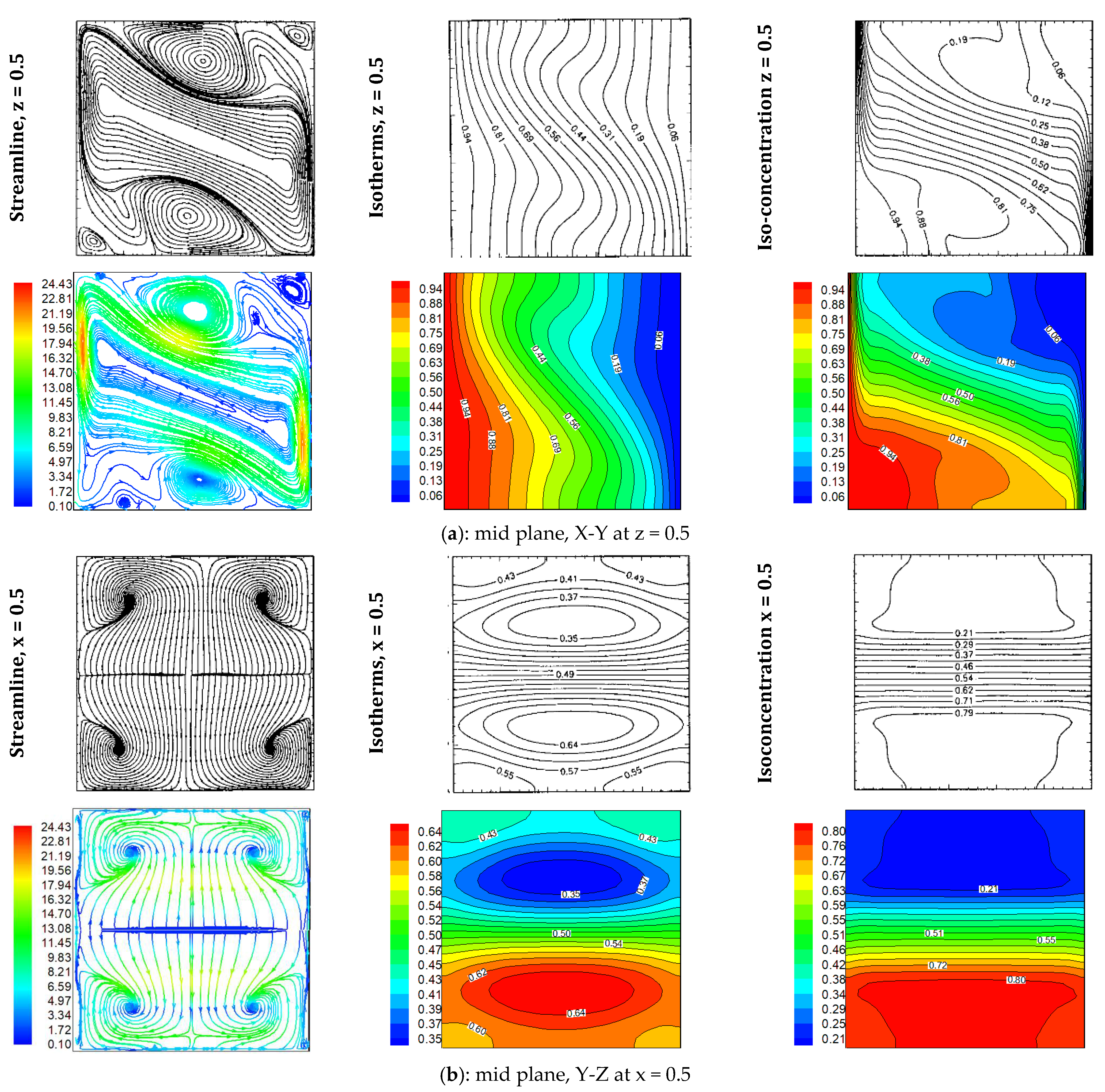
The numerical code was then verified by comparing the results with those obtained in two different simulation cases: the first case concerns a three-dimensional cavity with a horizontal gradient of temperature and concentration filled with an aqueous solution Pr = 10, Le = 10 and Ra = 10⁵ developed by Sezai and Mohamad [23], and the second one is related to a square cavity of dimension L filled with nanofluids containing a square hot obstacle centered in the cavity with a width W. The Prandtl number is equal to 6.2 and the Rayleigh number is equal to 10⁶. The nanofluid is water-Cu with a fraction of 0.04 [24] (

Table 3. Comparison of the obtained average Nusselt number with the results of Rahmati et al. [24] at Ra = 10⁶.

W/L	Nusselt Average, Rahmati et al. Works	Nusselt Average, Present Works	Error %
0.2	13	12.883	0.9
0.3	13.5	13.316	1.36
0.4	14	13.732	1.91
0.5	14.25	13.974	1.93
0.6	13.8	13.675	0.91

). It is clear that the results of our code are in good agreement with those proposed by Rahmati and Tahery [24]. Indeed, the maximum deviation is of the order of 1.8%. The flow structure, iso-concentration and iso-temperature obtained by our code are similar to those obtained by Sezai and Mohamad [23] in the two planes z = 0.5 and x = 0.5 (Figure 3).

5. Results and Discussion

The results presented in this paper were obtained for ranges of governing parameters: Rayleigh numbers (10³ to 10⁵), buoyancy (−2 to 2) and a barrier height (0.1 to 0.75). The Prandtl number was fixed at Pr = 0.7 and the Lewis number was Le = 1.2. Iso-concentration, iso-temperature and particle trajectories are presented to illustrate the dispersion of the contaminant, the effectiveness of the barrier and the heat and mass transfer in the building. Interesting results were seen for fluid flow and heat and mass transfer through the cavity, depending on the chosen values of the governing parameters, the sign of the buoyancy ratio and the height of the barrier.

5.1. Flow Patterns in Reference Case

The flow patterns in the reference case are studied in this subsection. The reference case is the case involving the building without a barrier.

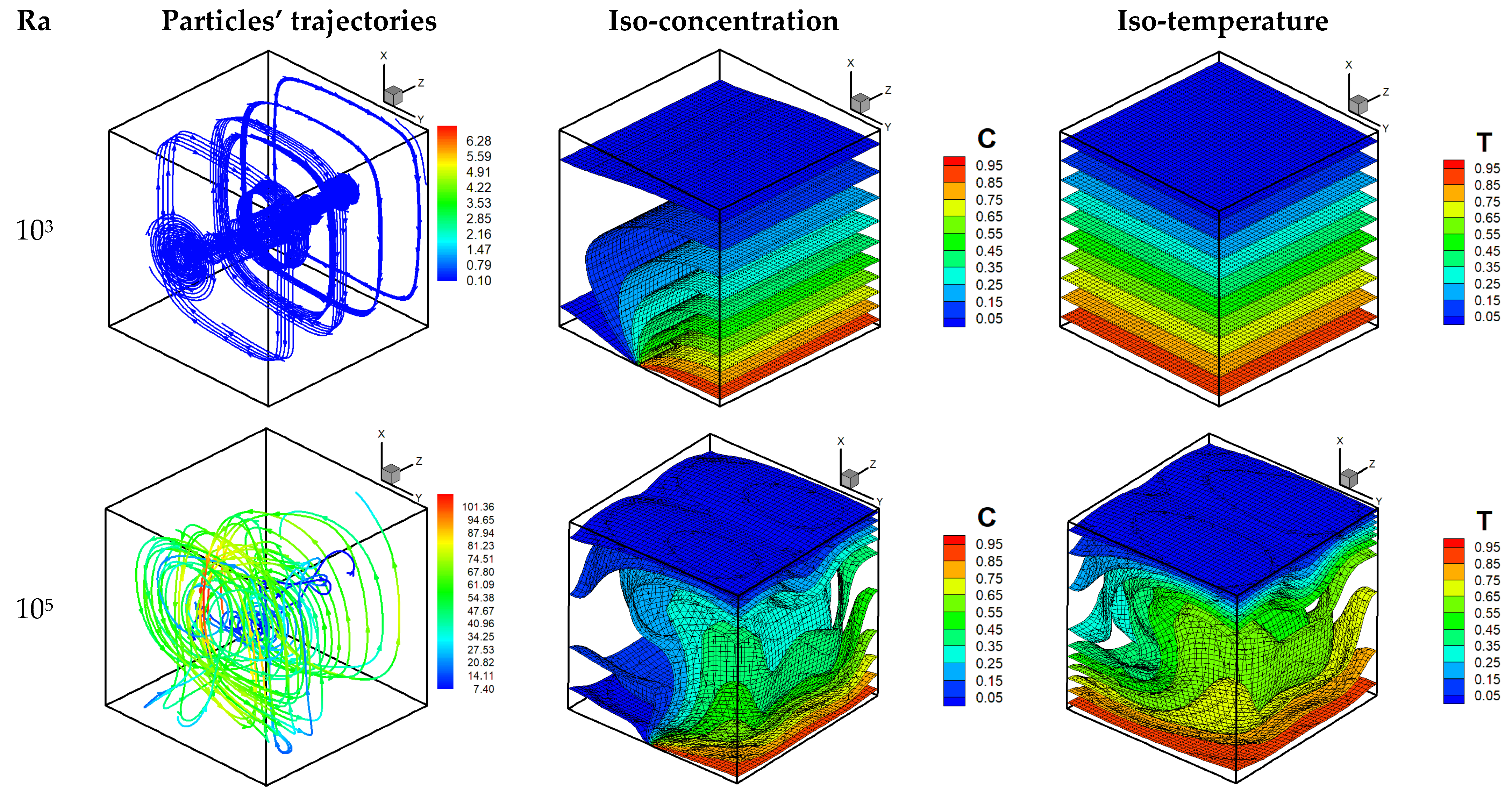
Figure 4 presents the particles trajectories, iso-concentrations and iso-temperatures at N = 0 for Ra = 10³ and 10⁵. The flow structure is characterized by a single clockwise rotating vortex. The contaminant particles move from the part at high concentration in the right bottom wall to the whole of the cavity due to the buoyancy forces. The increase of Rayleigh numbers increases the magnitude of fluid velocity without tangible variation of the flow structure. The distribution of iso concentration shows a diffusive dispersion on contaminant when Ra = 10³ is localized in the right side of the cavity due to the high concentration of the contaminant in the right building floor. The dispersion of the contaminant becomes convective when Ra = 10⁵. The dispersion of the contaminant is mainly directed upwards at the corners of the building and to the left in the core of the building. The iso-temperature structure shows that the conductive mode is dominant in case of Ra = 10³. When Ra = 10⁵, the thermal gradient increases and the convective mode becomes dominant.

5.2. Effect of Rayleigh, Barrier Height and Boyancy Ratio on the Dispersion of the Contaminant

5.2.1. Effect of Rayleigh and Barrier Height for N = 0

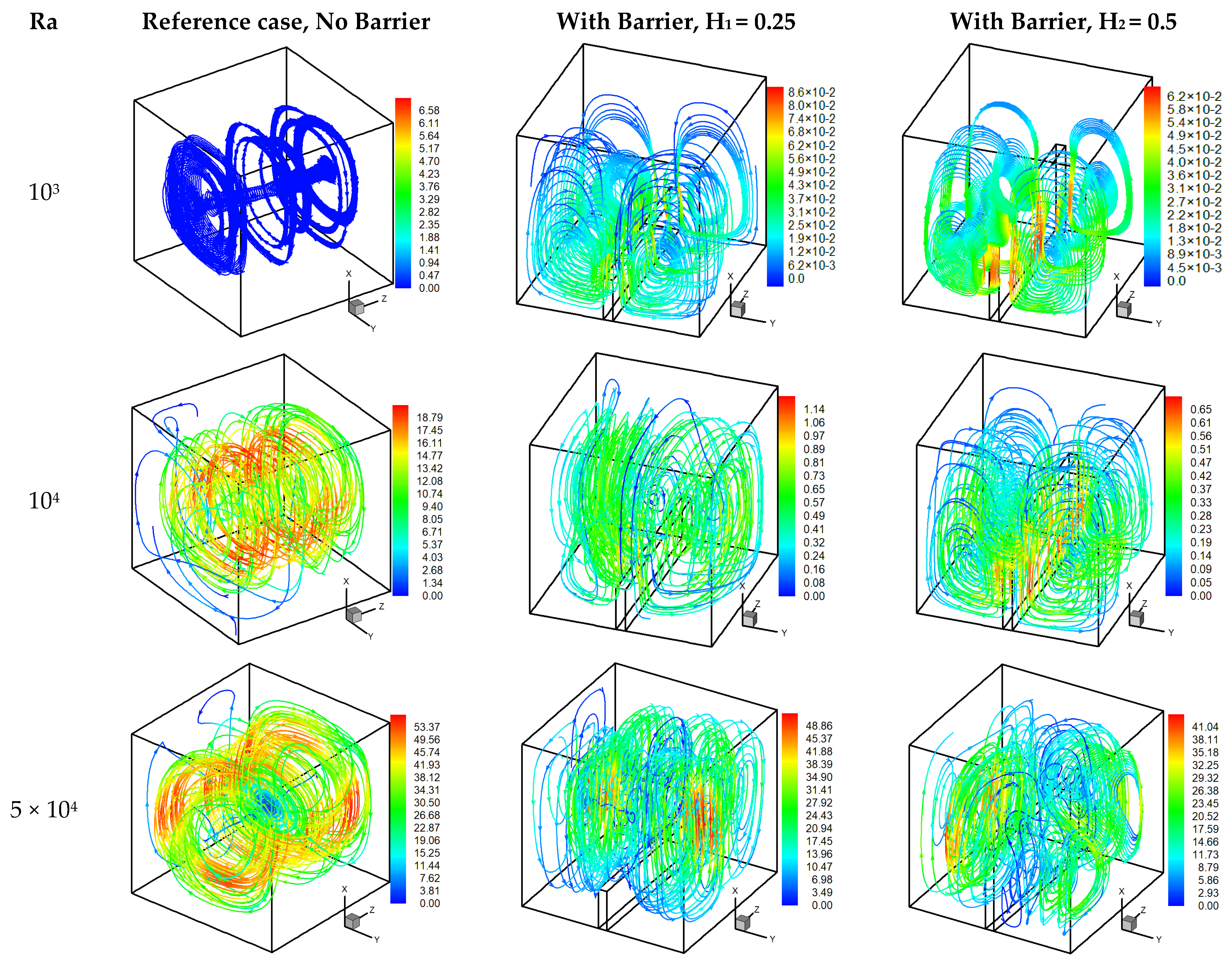
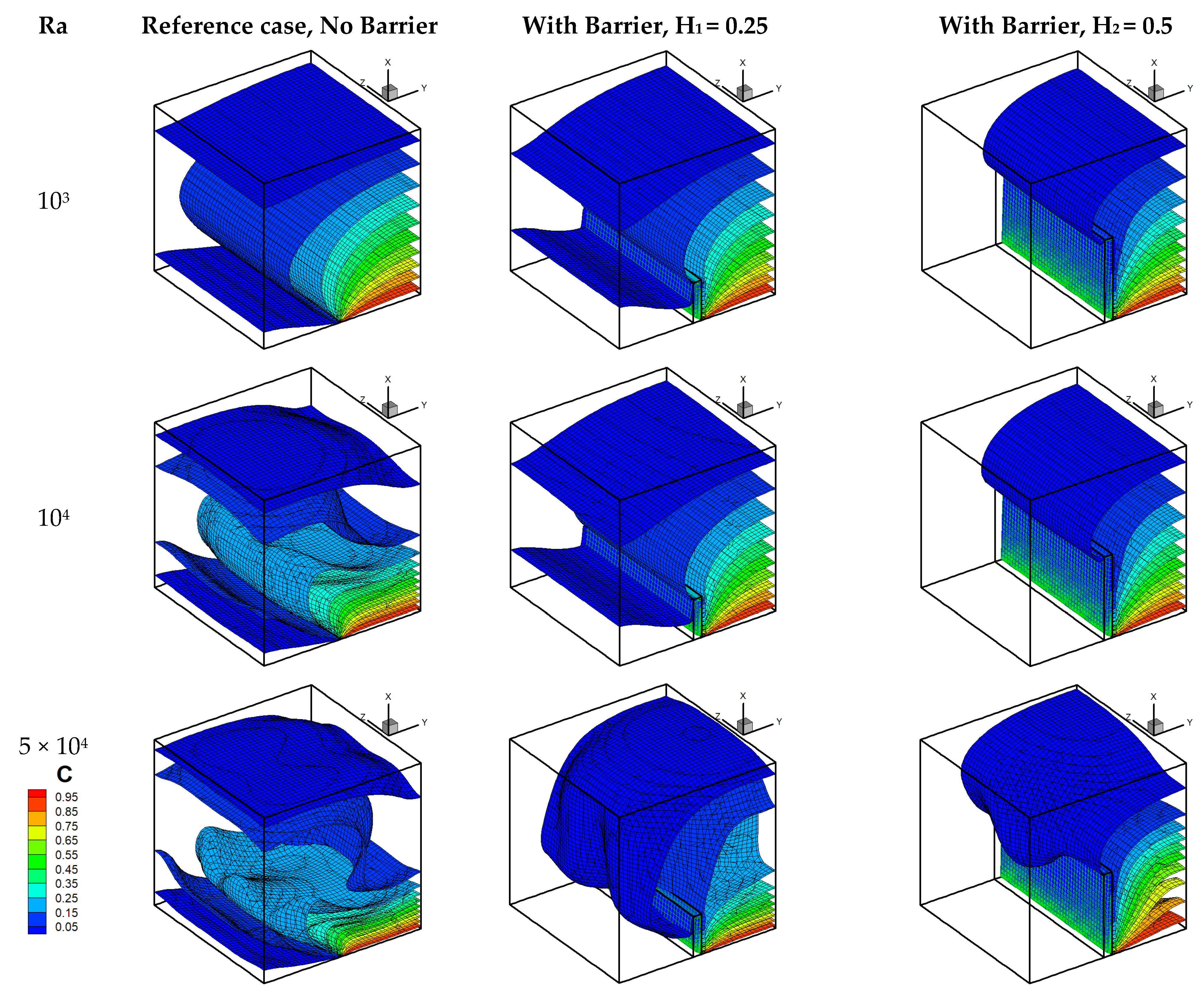
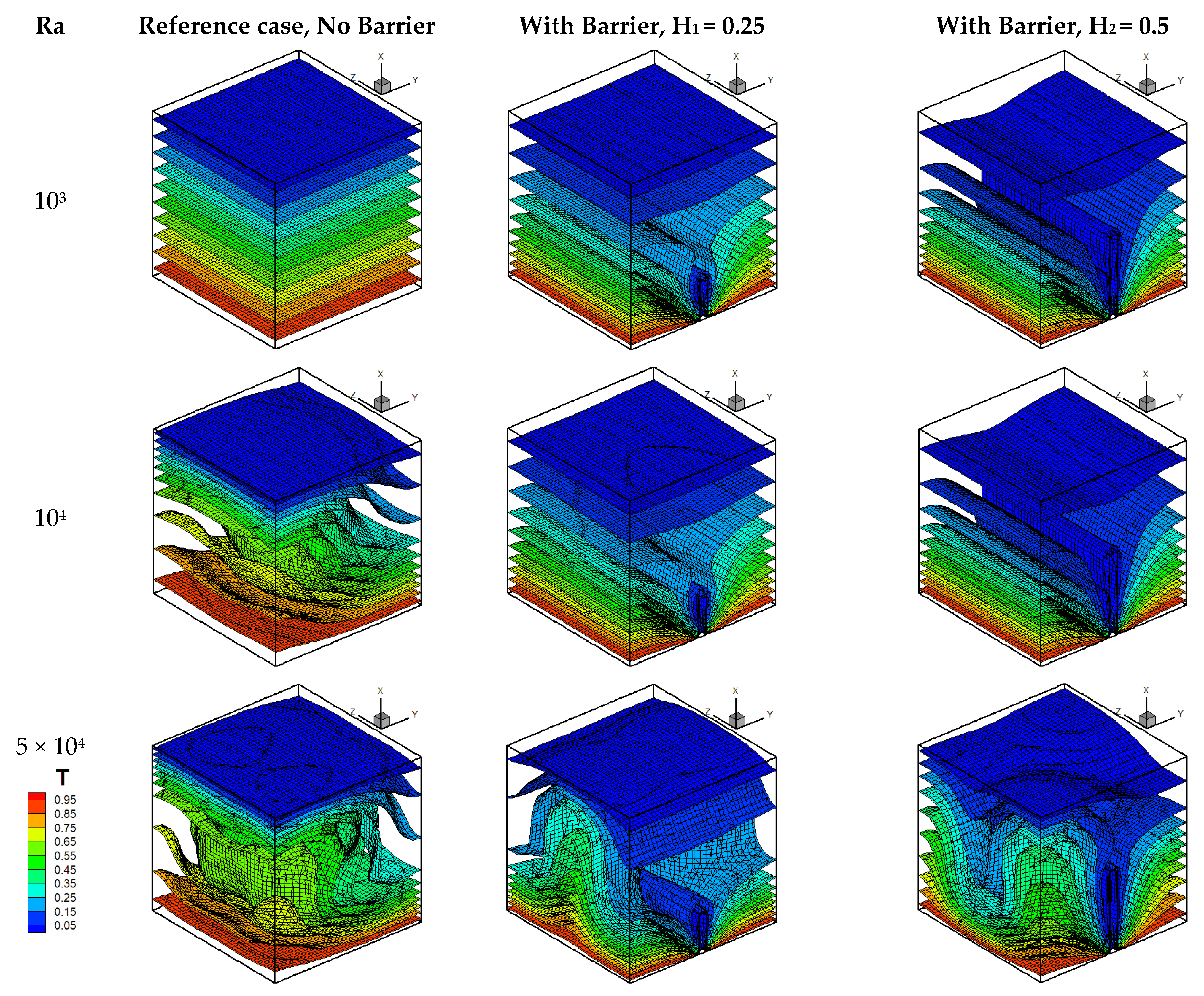
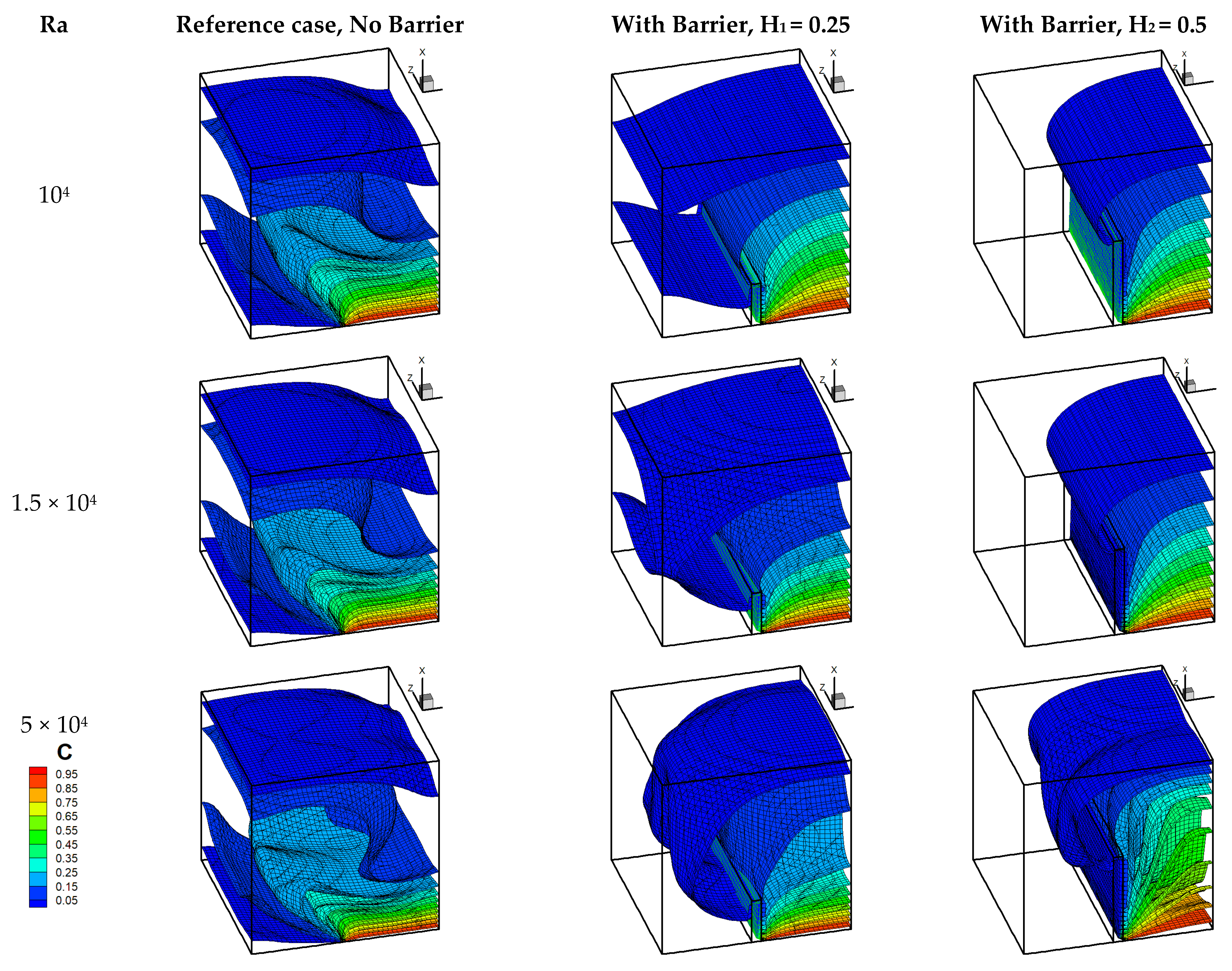
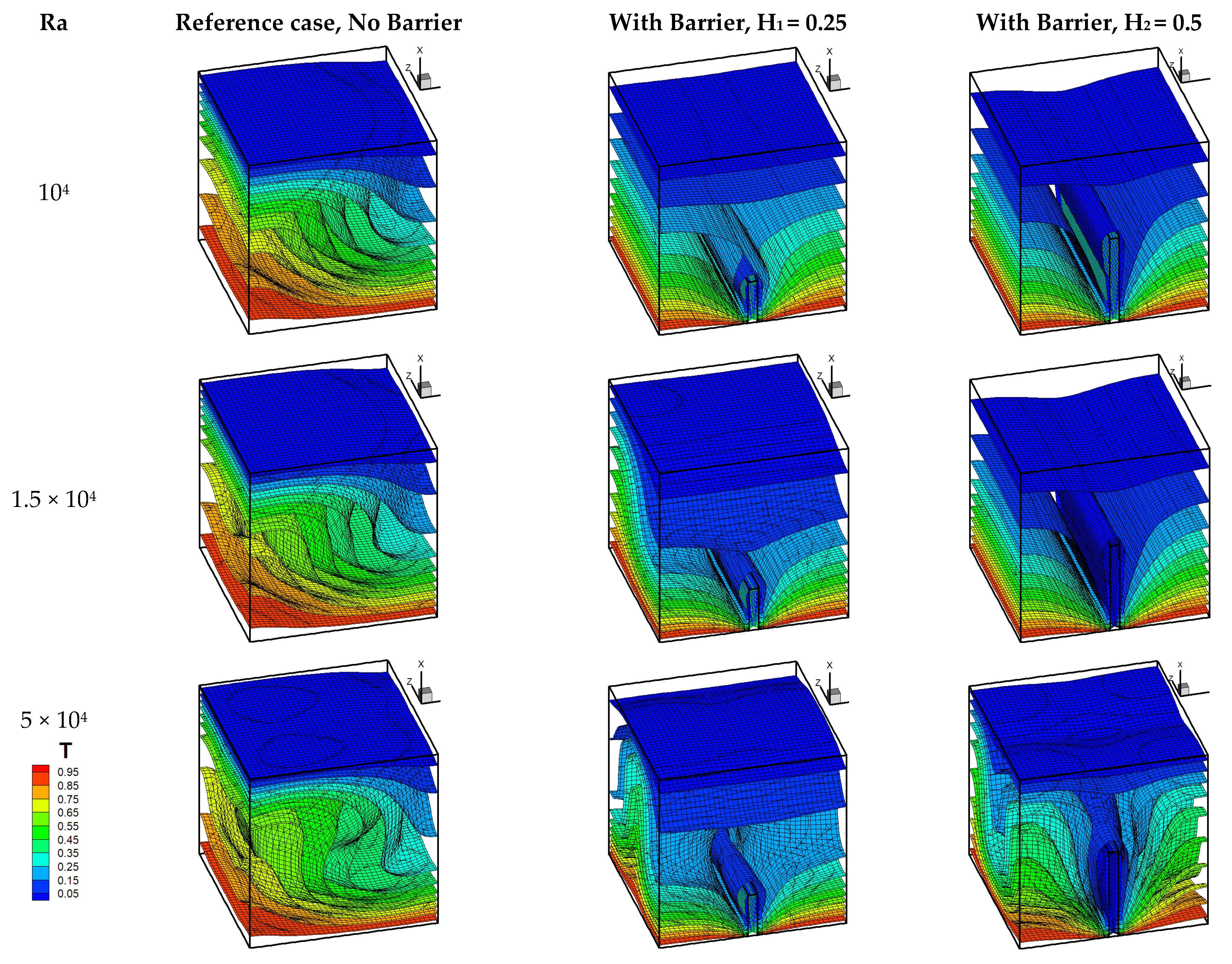
Figure 5, Figure 6 and Figure 7 presents the effect of barrier height on the contaminant flow dispersion, iso-concentrations and the iso-temperatures, respectively, for different Rayleigh numbers and N = 0. When the barrier is placed in the base wall of the cavity, the flow of fluid in the area to the right of the barrier is governed by thermal and solutal buoyancy forces. However, in the area to the left of the barrier, only thermal buoyancy forces govern the flow. Two heights of the barrier were studied in this work. The first height is 0.25 of the height of the cavity and the second is 0.5.

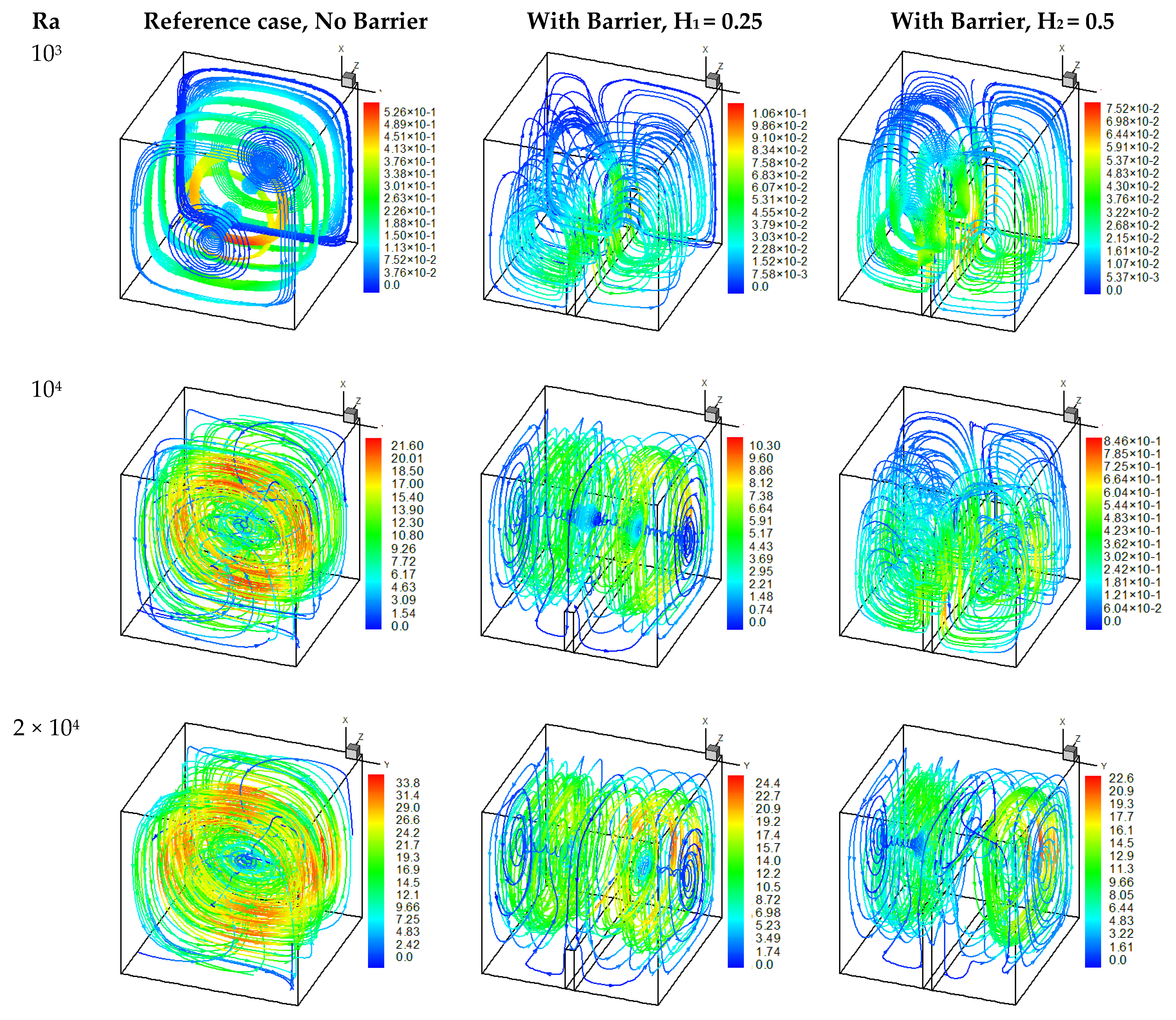
Figure 5 shows the effect of Rayleigh numbers on the flow structure in the building in three cases when N = 0; the first case represented in the first column is the barrier-free case (the reference case), the second case with the first height (0.25) whose results are presented in the middle column and the third case with the second height (0.5) in the third column. When Ra = 10³, it can be noticed that the presence of the barrier limited the dispersal of the contaminant throughout the cavity and that the magnitude of the velocity decreased remarkably compared to the case without the barrier (the reference case). It is also noticed that parallel flow rollers in the X-Y plane appeared when the barrier is installed. Additionally, at this Ra number, the effect of the barrier height cannot observed at the flow structure. However, a slight decrease in velocity can be observed when the barrier height is at its maximum. For Ra = 10⁴, there is a noticeable change in the flow structure for the first obstacle height, and the flow structure is characterized by parallel rotating vortices in the X-Z plane. The flow structure is almost similar on both sides of the obstacle with slight differences, which is represented by the presence of small vortices positioned at the bottom in the right side of the cavity. On the other hand, for the second height of the obstacle, the flow structure is not changed, and only a slight increase in the velocity can be noticed.

When Ra = 5 × 10⁴, it can be observed that the velocity of the flow is further increased and in the absence of the barrier, the contaminant is dispersed in the whole cavity. Thus, the main flow always comprises of a single central vortex that encloses the entire volume with a spiral flow. The increase in the Rayleigh number for the case of the first barrier height induced a second change in the flow structure compared to the Ra = 10⁴. In this case, the flow pattern is recognized by two vortices rotating in opposite directions in the X-Z plane. The flow structure is similar on both sides of the barrier. The increase in the Rayleigh number in the cavity with the second height of the barrier also induced a change in the flow structure compared to Ra = 10³ and Ra = 10⁴. In this case too, the flow structure is characterized by two counter-rotating vortices in the X-Z plane on the right side of the barrier, while it is a single vortex on the left side. Such differences in the flow structure between the two sides of the barrier may be related to the combined effects of the thermal and solutal volume forces on the right side compared to the single thermal effect on the left side.

Figure 6 illustrates the effect of Rayleigh numbers on the iso-surfaces of contaminant concentration in the building in the three cases studied. When Ra = 10³, the concentration iso-surfaces are distributed from the contaminant emitting area. They are parallel and located in the right part of the cavity. The solutal gradient is low and the diffusive regime is dominant. The diffusion of the contaminant is mainly directed towards the top of the cavity by migration under the influence of the side walls. For Rayleigh numbers equal 10⁴ and 5 × 10⁴, on the one hand an increase in the solutal gradient can be noticed while on the other hand a convective effect appears. The contaminant starts to disperse horizontally towards the left part of the cavity and contaminates the remaining parts of the cavity too. The implementation of the barrier shows an effect limiting the horizontal dispersion of the contaminant. For both Rayleigh numbers i.e., 10⁴ and 5 × 10⁴, it can be concluded that the second height strongly opposes the dispersion of the contaminant. The convective effect is attenuated by the presence of the barrier and pushes the contaminant to only migrate vertically near the side walls.

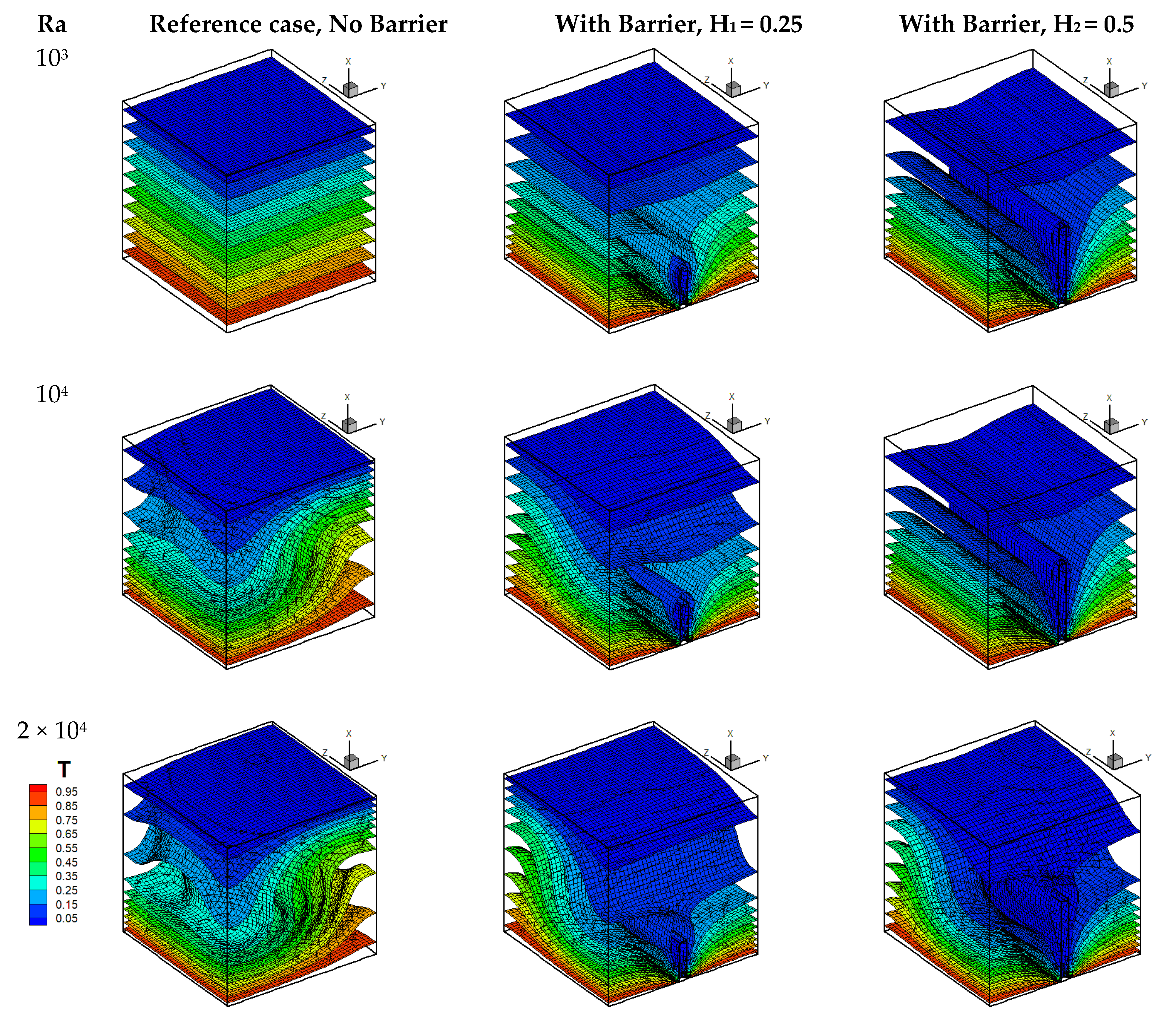
Figure 7 shows the effect of Rayleigh numbers on temperature iso-surfaces. In the absence of a barrier and when Ra = 10³, it can be noticed that the temperature iso-surfaces are parallel and that the conductive regime is dominant. The thermal convective regime appears from the value of Ra = 10⁴, as evidenced by the distribution of the temperature iso-surfaces that start to deform from the side in the cavity that has a higher thermal gradient with the source of contamination. For Ra = 5 × 10⁴, the temperature iso-surfaces form an S-shape, indicating the complete development of the thermal convective mode. In the presence of the barrier and for both Rayleigh numbers 10³ and 10⁴, it can be noticed that the distribution of temperature iso-surfaces is similar and characterized by a dominant conductive thermal regime. Also, the thermal gradient is weak on both sides of the barrier. When Ra = 5 × 10⁴, complete development of the thermally convective mode can be seen. It can further be observed that the structure of the temperature iso-surfaces depends on the height of the barrier. Indeed, for the first height of the barrier, the thermal gradients are high at the corners of the cavity and low in the middle part. However, for the second height, it can be noticed that they are low at the corners and high in the middle.

5.2.2. Effect of Rayleigh and Barrier Height for N = −0.2

The nature of the contaminant and its characteristics have a major effect on the manner of its dispersal. For the case where the contaminant is in a liquid sprayed phase loaded with viruses or bacteria and is bound to its environment during its emission and dispersion, the dispersion of this existing viral load in the pulverized liquid phase is then governed by gravity having a descending effect, which is opposed to the effect of natural convection. In this case, the effects of the forces of solutal and thermal volumes are then opposed. This situation can be modeled with the negative buoyancy ratio.

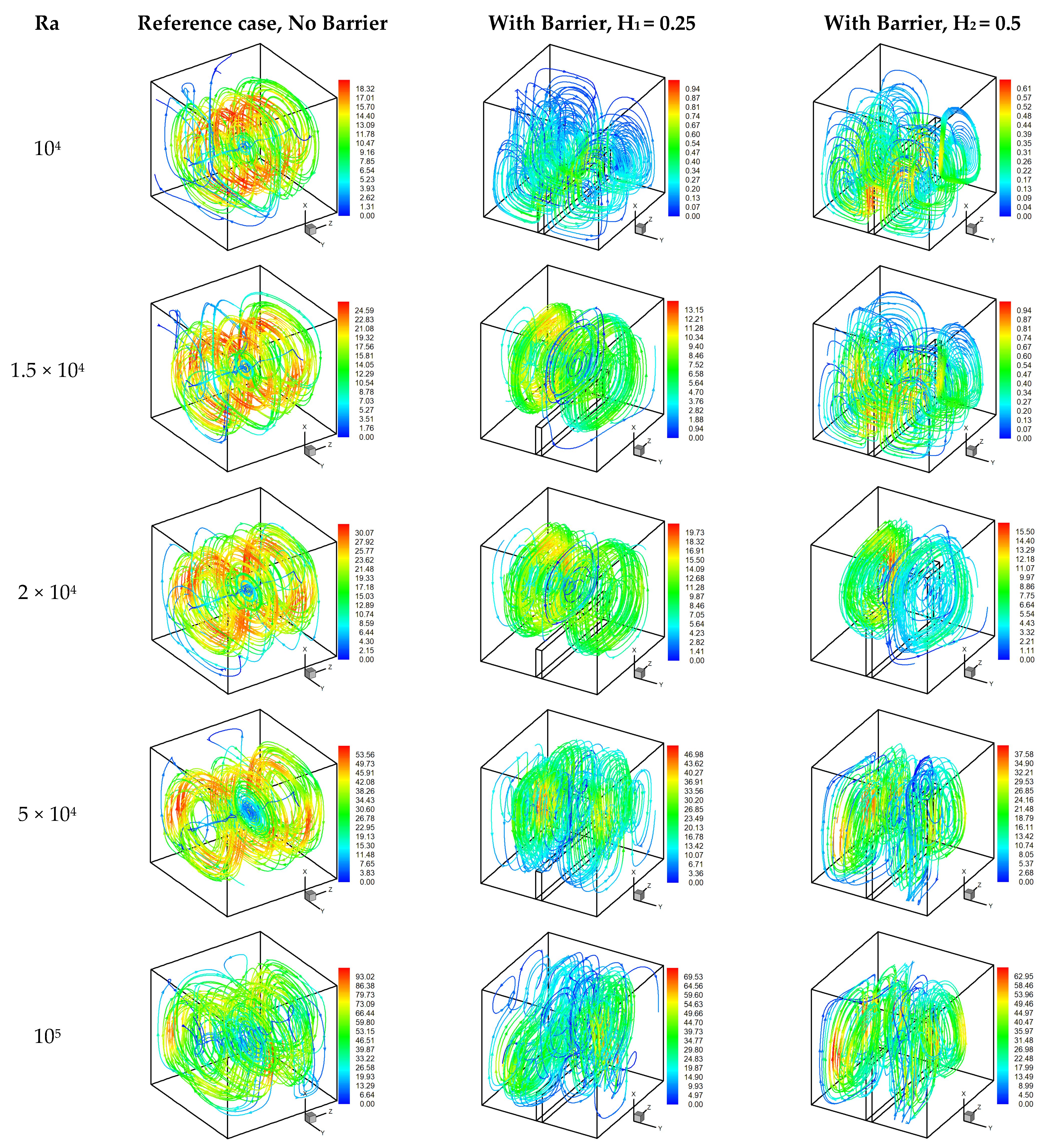
Figure 8 presents the effect of Rayleigh numbers on the flow structure represented by particles’ trajectories in the building in the three cases of this study when N = −0.2. For all Rayleigh numbers, the flow structure in the reference case is characterized by a single vortex in the X-Y plane rotating in a clockwise direction. Increasing the Rayleigh number increases the flow velocity. When the building is equipped with the barrier, it is noticed that the variation of the Rayleigh number has a double effect on the flow structure as well as on the flow velocity.

When Ra = 10⁴, the flow structure is similar in both cases, as shown by barrier height 1 and 2. Indeed, the flow is then characterized by two vortexes rotating in opposite directions: one on left of the barrier and the other on the right. The one on the right, where the contaminant’s emitting surface is, the vortex rotates in a counterclockwise direction. On the other hand, the vortex on the left rotates in a clockwise direction. The increase in the Rayleigh number to 1.5 × 10⁴ causes a change in the flow structure in the case of height 1 of the barrier, and this flow structure remains unchanged in the case of height 2. The flow structure is characterized by a vortex rotating in the core of the X-Z plane, turning counterclockwise. It is from Ra = 2 × 10⁴ that the flow structure in the second height of the barrier has this new structure. It can also be noticed that the magnitude of the particle velocity is lower on the right side of the barrier, on the side of the contaminant emitting surface when compared to the left side.

When Ra = 5 × 10⁴, the flow structure changes again in both cases and becomes characterized by two oppositely rotating vortexes carried by rollers in the Y-Z plane along the entire cavity. It can be noticed that the intensity of the velocity is lower on the side of the contaminant emitting surface compared to the region to the left of the barrier. This result can be explained by the competition between the thermal and solutal volume forces in the zone on the right side of the barrier, as the negative buoyancy ratio. In contrast, only the thermal volume forces govern the flow in the zone on the left side of the barrier. When Rayleigh number is equal to 10⁵, it can be noticed that the flow structure for the first case becomes multicellular. The flow velocity has increased in both cases and the maximum velocities are observed in the zone to the left of the barrier where only the forces of thermal volumes govern the flow.

Figure 9 presents the effect of Rayleigh numbers for N = −0.2 on the iso-surface of contaminant concentration in the building for the three cases in this study. The increase of the Rayleigh number in the reference case, the building without barriers, increases the concentration gradient close to the contaminant emitting surface. The structure of the iso-surfaces shows that the solutal convective effect is predominant. The increase of the Rayleigh number also increases the dispersal effect of the contaminant mainly in a horizontal way at the bottom of the building. It can be noticed that the placement of the barrier with height 1 reduces the dispersion of the contaminant towards the left zone. For the low Rayleigh number, the dispersion is horizontal, under the effect of diffusion, which is the dominant regime. For Ra = 5 × 10⁴, it can be noticed that the dispersion of the contaminant becomes governed by the solutal convection. It can be noticed that the second height of the barrier is more effective in terms of limiting the dispersion of the contaminant towards the left zone. However, it can be observed that this case has led to an increase in the vertical dispersion of the contaminant compared to the other studied cases.

Figure 10 shows the effect of Rayleigh numbers on temperature iso-surfaces. In the absence of a barrier, the thermal convective regime appears from the value of Ra = 10⁴, while increasing the Rayleigh number increases the thermal gradient. In the presence of barrier height 1, the convective regime appears from Rayleigh 1.5 × 10⁴, while for barrier height 2, the convective regime is observed for Ra = 5 × 10⁴.

5.2.3. Effect of Rayleigh and Barrier Height for N = 0.2

When the contaminant is a volatile organic compound (VOCs), then its emission and dispersion are caused by its volatilization having an ascendant effect. In this case, the thermal and solutal volume forces act in the same direction. This situation is modeled by a positive volume force ratio, which is the subject of this section. In this section, the flow structure, iso-concentration and iso-temperatures in the case of N = 0.2 are presented.

Figure 11 shows the effect of the barrier on the particle trajectory for three Rayleigh values. When the cavity is barrier-free, the flow structure is characterized by a vortex encompassing the cavity in the X-Y plane and rotating counterclockwise. Increasing the Rayleigh number increases the magnitude of the flow velocity. In general, and for all Rayleigh number values, the installation of the barrier decreases the flow velocity in the cavity. It can also be noticed that barrier 2 has a more pronounced effect on the flow attenuation. For Ra = 10³, for both cases of barrier height, the flow structure is characterized by two vortexes in the X-Y plane separated by the barrier and turning in the opposite direction.

A modification of the flow structure is observed for barrier 1 (the barrier with a height equal to H₁) from Ra = 10⁴ and for barrier 2 when Ra = 2 × 10⁴. In fact, the flow structure is characterized by a vortex with spiral character carried in the X-Z plane and turning counterclockwise.

It can also be noticed that in the presence of the barrier, the increase of the Rayleigh number has a double effect on the change of the flow structure and on the velocity magnitude. However, the increase of the velocity intensity is correlated to the direction and the plane of the vortex rotation. For barrier 1, it can be noticed that when Ra increases from 10³ to 10⁴, there is a change in the flow structure where the vortexes become located in the X-Y plane and a high increase in the velocity magnitude of up to 100 times occurs. The velocity magnitude is only 10 times in the case of barrier 2 where the flow structure has not undergone a great change. As Ra increases from 10⁴ to 2 × 10⁴, the change in the plane of rotation of the vortexes can be observed for barrier 2 and is associated with an increase in the velocity magnitude by 30 times. However, this increase is only by 2 times in the case of barrier 1 where the flow structure has not changed.

This correlation between the change of the plane carrying the vortices and the velocity magnitude can also be observed in the case of N = −0.2 (Figure 8) where the impact of the velocity increase is of the order of 15 times. This correlation can be observed for Ra = 1.5 × 10⁴ in barrier 1 and Ra = 2 × 10⁴ in barrier 2. These observations show that the flow has a strong three-dimensional character.

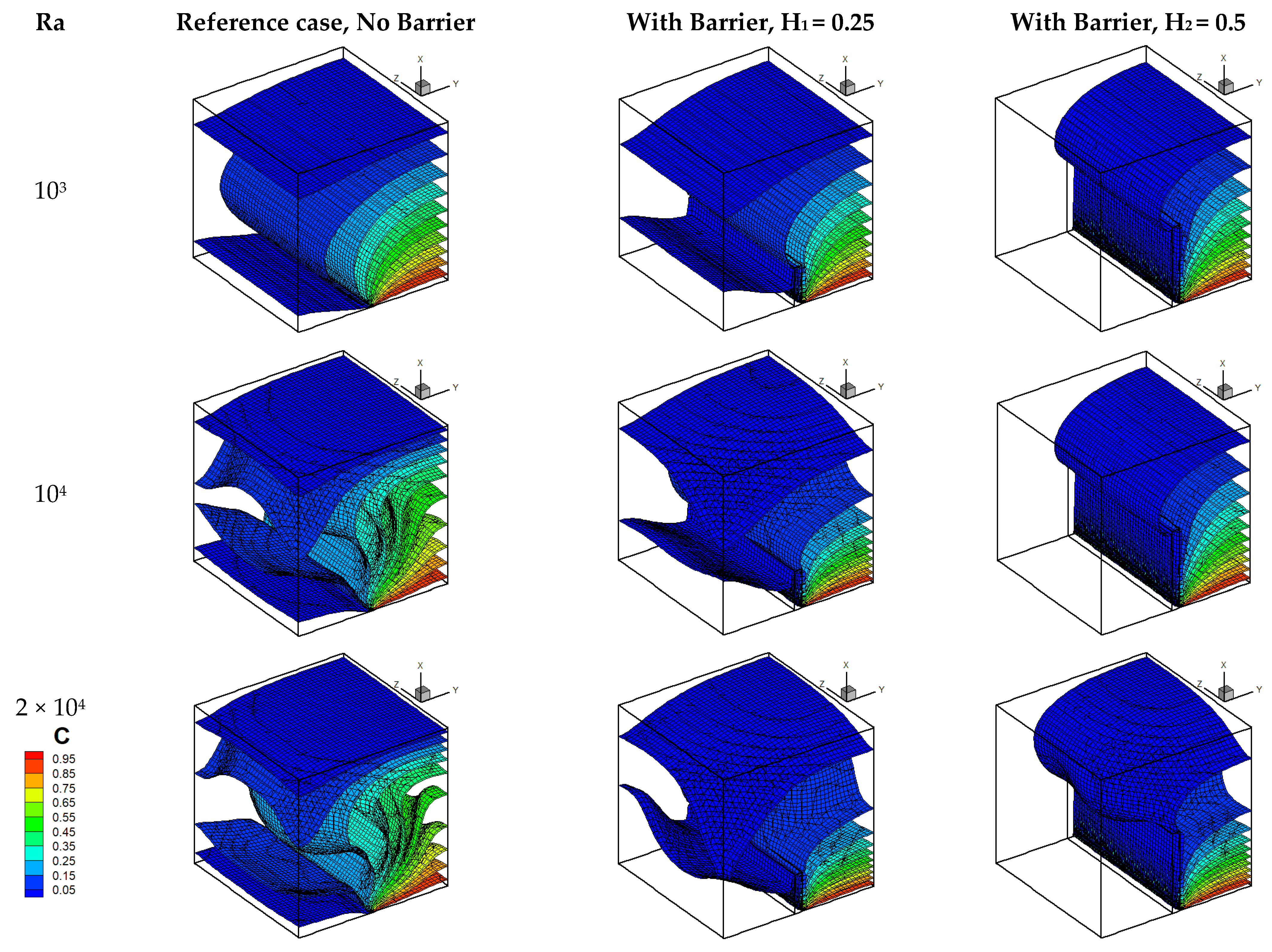
Figure 12 shows the effect of the barrier and Rayleigh number on the contaminant iso-surfaces of concentration. For Ra = 10³, the iso-concentrations are parallel, showing a dominant diffusive regime. The barrier has no significant effect on the solutal gradient. The height 2 allows an isolation of the dispersion of the concentration towards the left zone. The last finding is also observed when Ra = 10⁴. However, from this number of Ra = 10⁴, a convective solutal regime is noticed for the reference case, and the variation of the height of the barrier only affects the solutal gradient for Ra = 10⁴.

Figure 13 shows the isotherms for the case N = 0.2. It can be seen that the thermal convective effect appears in the cavity from Ra = 10⁴. The presence of the barrier has caused a change in the isotherm structure. Indeed, the variation of the thermal gradient is initially a function of y, though it becomes a variable according to z. It can also be observed that the thermal gradient is weaker on the side of the contaminant source compared to the other side.

5.3. Efficiency of Protective Barrier and Heat-Mass Transfer Ratios

5.3.1. Barrier Efficiency

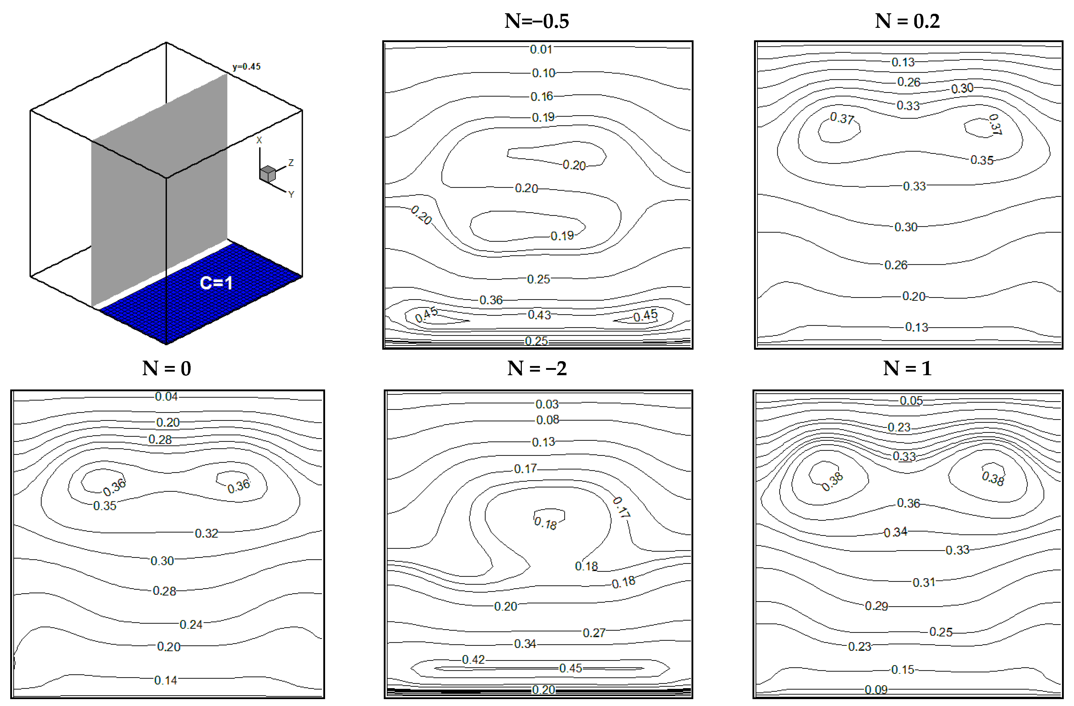
To study the efficiency of the barrier in reducing the dispersion of the contaminant from the region containing the contaminant source to the region on the left, the analysis focused on the evaluation of the concentration of the contaminant in the plane y = 0.45, where the plane is very close to the limit of the contamination surface (Figure 14). In this plane, we looked for the maximum contaminant concentration observed in the case of a building with and without a barrier. It can be noticed that the coordinates of the maximum concentration depend on the buoyancy ratio, Rayleigh number and time. For the positive buoyancy ratio, the maximum concentration is located at the top, but for the negative value, it is located at the bottom, and the concentration distributions have a three-dimensional character.

The barrier efficiency is defined by this relation $E_{ff}=1-\frac{c_{max}}{C_{max0}}$, where $c_{max}$ is the maximum contaminant concentration in the plane y = 0.45, for the building with a barrier. Also, $c_{max0}$ is the maximum contaminant concentration in the plane y = 0.45, for the reference building without a barrier.

Figure 15 shows the effect of the Rayleigh number on the efficiency of the barrier for two heights H₁ = 0.25 and H₂ = 0.5. A minimum efficiency equal to 36.22% can be observed for height 1, Ra = 10⁴ and N = 0.2. Meanwhile, the maximum efficiency (85.18%) can be observed for height 2, Ra = 1.5 × 10⁴ and N = −0.2. For height 1 and when N = 0.2, the increase in Ra decreases the efficiency up to Ra = 10⁴, reaching a minimum, then the increase in efficiency takes on a positive slope, and the percentages increase with the increase of Ra. When N = −0.2, it can be observed that going from Ra = 10³ to 10⁴, the efficiency increases from 50% to 60% and then decreases to 52% for Ra = 1.5 × 10⁴ before it resumes its positive slope and reaches more than 75% for Ra = 10⁵.

For height 2 and when N = 0.2, the increase of Ra from 10³ to 10⁴ has no effect on the efficiency of the barrier and it is starting from Ra = 1.5 × 10⁴ that we can observe a decrease reaching a minimum equal to 64%, which was observed for Ra = 2 × 10⁴. From this value, an increase in Ra increases the efficiency. When N = −0.2, a slight increase in efficiency is observed from Ra = 10³ to 1.5 × 10⁴, reaching a maximum equal to 85.18%. From this value, the increase in Ra values decreases the efficiency.

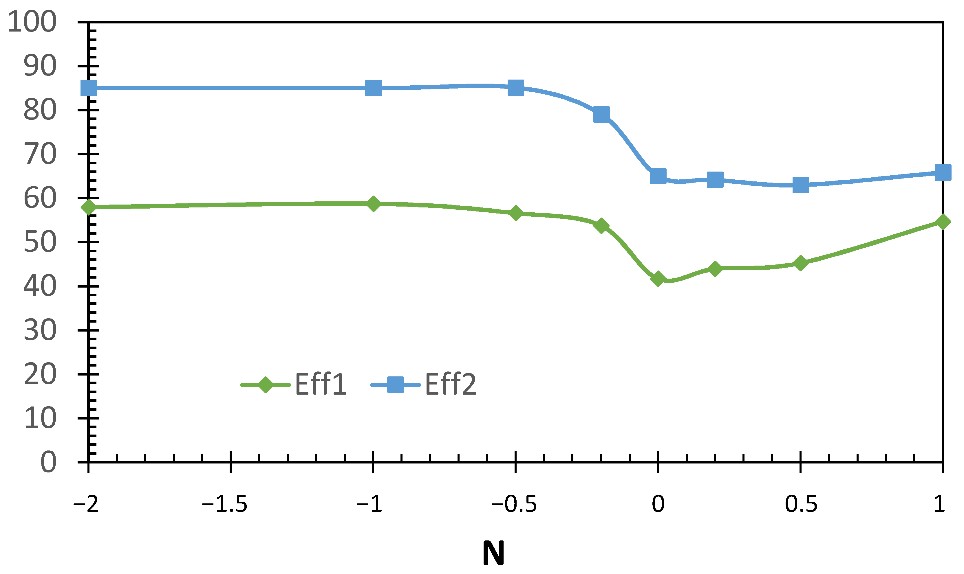
Figure 16 shows the effect of the buoyancy ratio on the efficiency of the barrier when Ra = 10⁴. It can be observed that the increase in the efficiency as a function of N is similar for the two heights of the barrier H₁ and H₂. The efficiency is 85% for H₂ and all negative values of N under −0.5, and it is 57% for H₁. From this value of N = −0.5, a decrease in the efficiency can be noticed, reaching a minimum equal to 41.67% at N = 0 for H₁ and 62.96% at N = 0.5 for H₂. Then the increase in the efficiency takes on a positive slope with the increase of N. The barrier efficiency percentages are higher for negative buoyancy ratios than for positive ones.

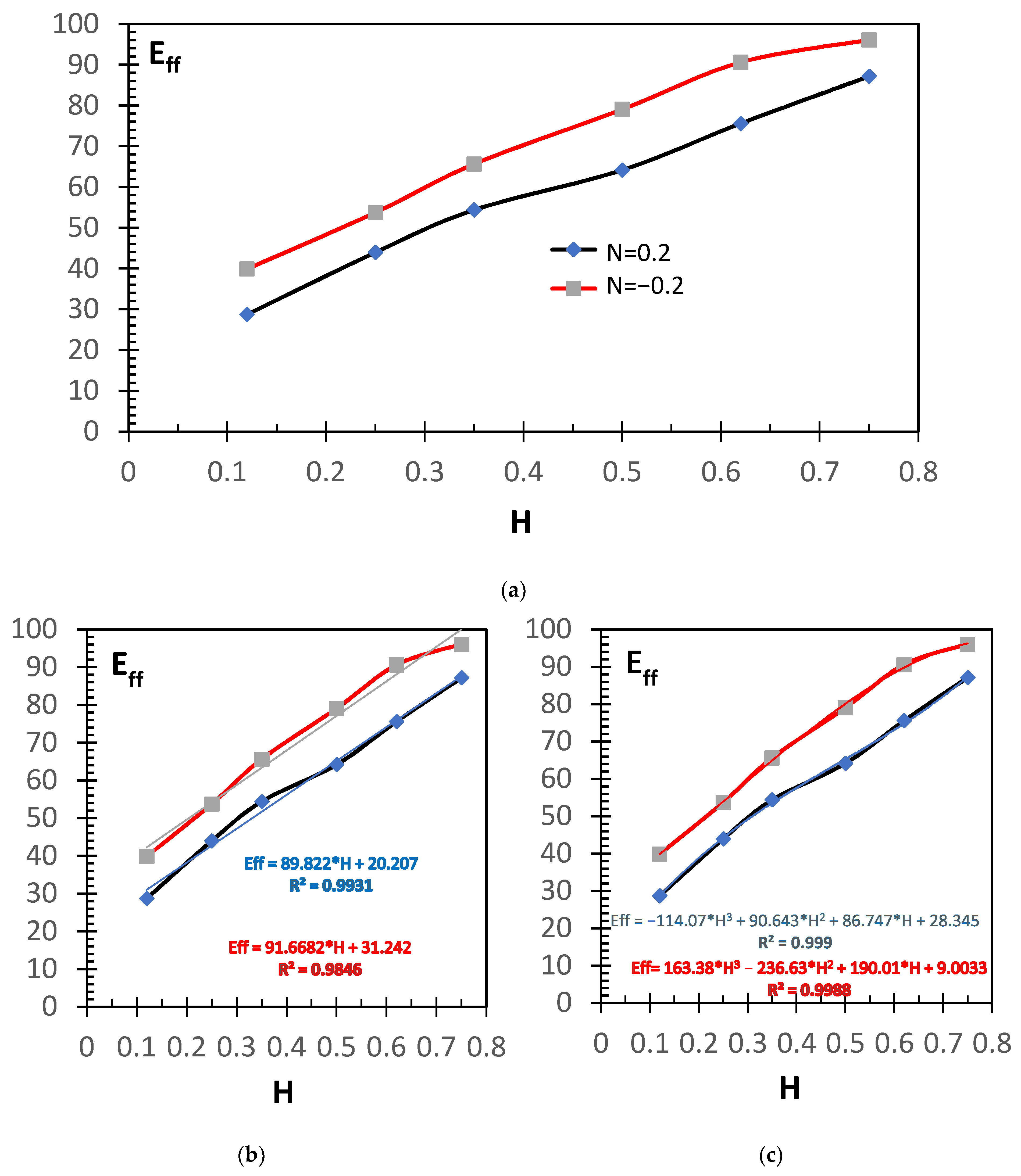
Figure 17a shows the effect of the barrier height on efficiency for Ra = 2 × 10⁴, N = 0.2 and N = −0.2. For all values of H, the efficiencies for N=−0.2 are higher than those for N = 0.2. For N = 0.2, the trajectory can be divided into two parts; from H = 0.12 to H = 0.35, the slope of the curve is 111.61, but from H = 0.35 to 0.75, the slope decreases and becomes 81.96.

For N = −0.2, the efficiency pattern follows three slopes: the highest one is from H = 0.12 to 0.35, and it is 112.02, the second one is from 0.35 to 0.62 and it is 76.15 and the third one is the lowest one of 42.19 from 0.62 to 0.75. In this latest range, the efficiency goes from 90% to 96%.

To further analyze the efficiency variation as a function of height, the two curves for N = 0.2 and N = −0.2 are treated by adding a trendline (Figure 17b,c). Two forms of equations are examined: linear (Figure 17b) and polynomial (Figure 17c) and the $R^2$ trendline reliability for each equation is compared. It can be found that the polynomial variation of order 3 gives a better reliability trendline, closer to 1. So, we can conclude that the efficiency increases following a polynomial evolution of order 3 as $E_{ff}=C_1{H}^3+C_2{H}^2+C_{3}H+C_4$ and that the constants $C_1,C_2,C_3\mathrm{and}{C}_4$ depend on the Rayleigh and N numbers.

5.3.2. Heat and Mass Transfer Ratios

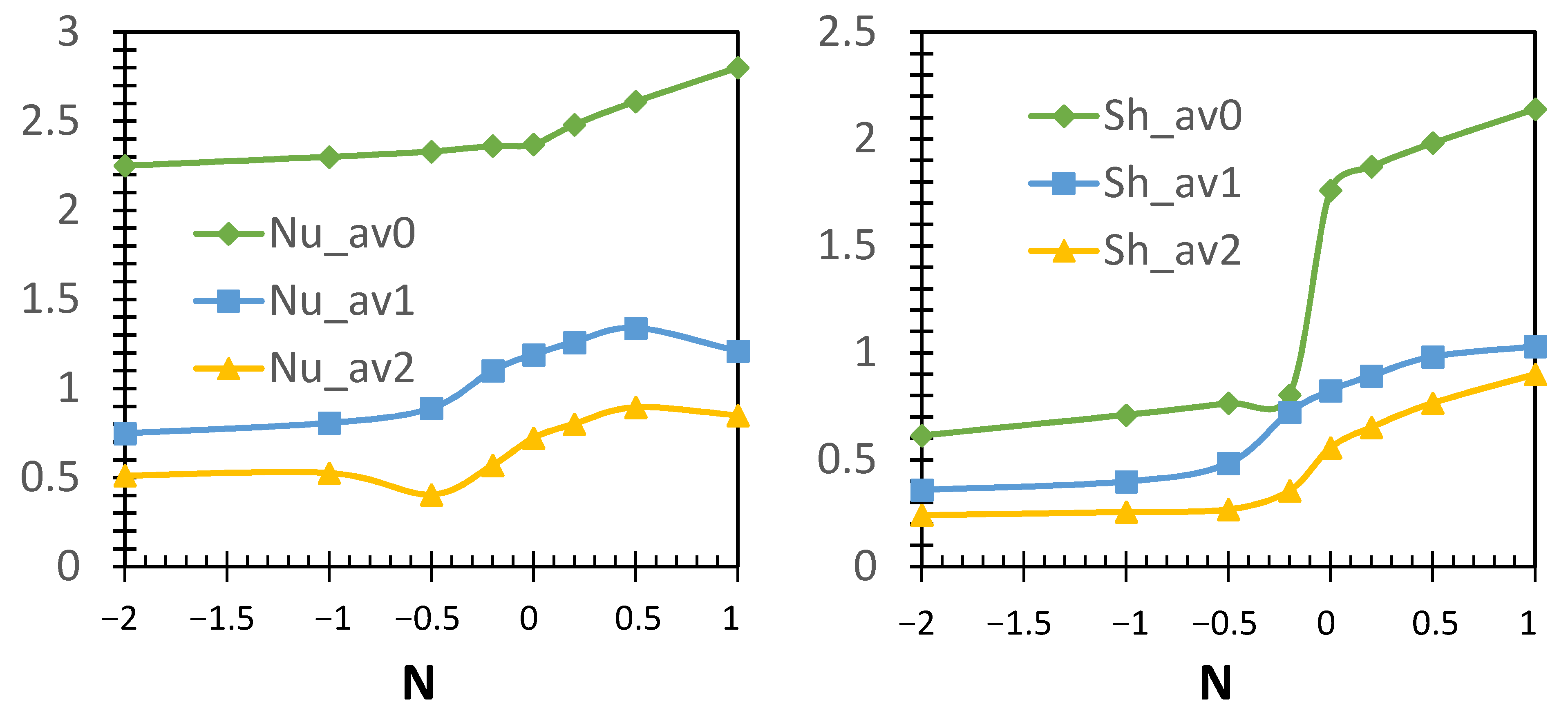
Figure 18 shows the effect of the buoyancy ratio on the heat and mass transfer ratio for Ra = 2 × 10⁴ for three cases: (0) considered as a reference without a barrier, (1) case of barrier height H₁ and (2) for H₂. It can be noticed that the presence of the barrier decreases the heat and mass transfer rates. The average Nusselt number in the reference case increases with two slopes. An increase in the slope of the average Nusselt number is observed from N = 0. For a barrier of height H1, the variation is parabolic with a maximum at N = 0.5. The average Nusselt number for the case of height 2 with a minimum variation is observed at N = −0.5 while the maximum occurs at N = 0.5. For a negative buoyancy ratio values, the increase in N has no significant effect on the average Sherwood number for the different cases studied. From N = −0.2 onwards, an increase in the mass transfer rate is noticed.

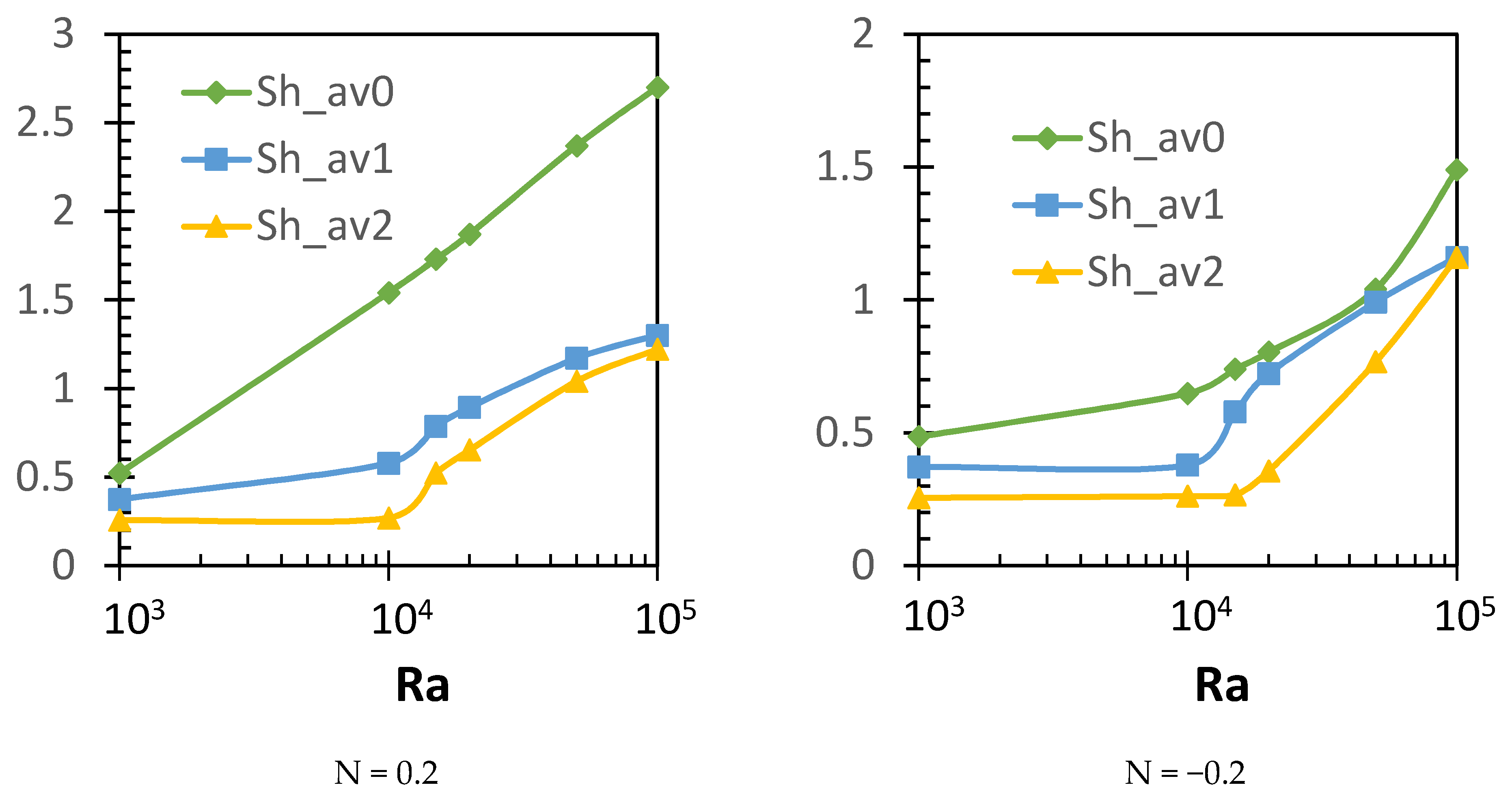
Figure 19 presents the effect of the Rayleigh number on the average Sherwood number for N = 0.2 and N = −0.2. When N = 0.2, there is a linear increase in the average Sherwood number as a function of Ra for the reference case. When the barrier is placed, the average Sherwood number changes in two incremental steps. When Ra is less than 10⁴, a slight increase in the mass transfer rate is observed. From this value, the increase of average Sherwood number is more than double when Ra = 10⁵.

When N = −0.2, the trajectory of the average Sherwood number variation is similar for the different cases studied. From Ra = 10³ to 10⁴, the mass transfer rate is almost constant with a slight increase observed for the reference case. From Ra = 10⁴, the increase in Ra significantly increases the average Sherwood number for the three cases studied. For Ra = 5 × 10⁴, it can be observed that the average Sherwood number for the reference case is nearly equal to that for the H₁.

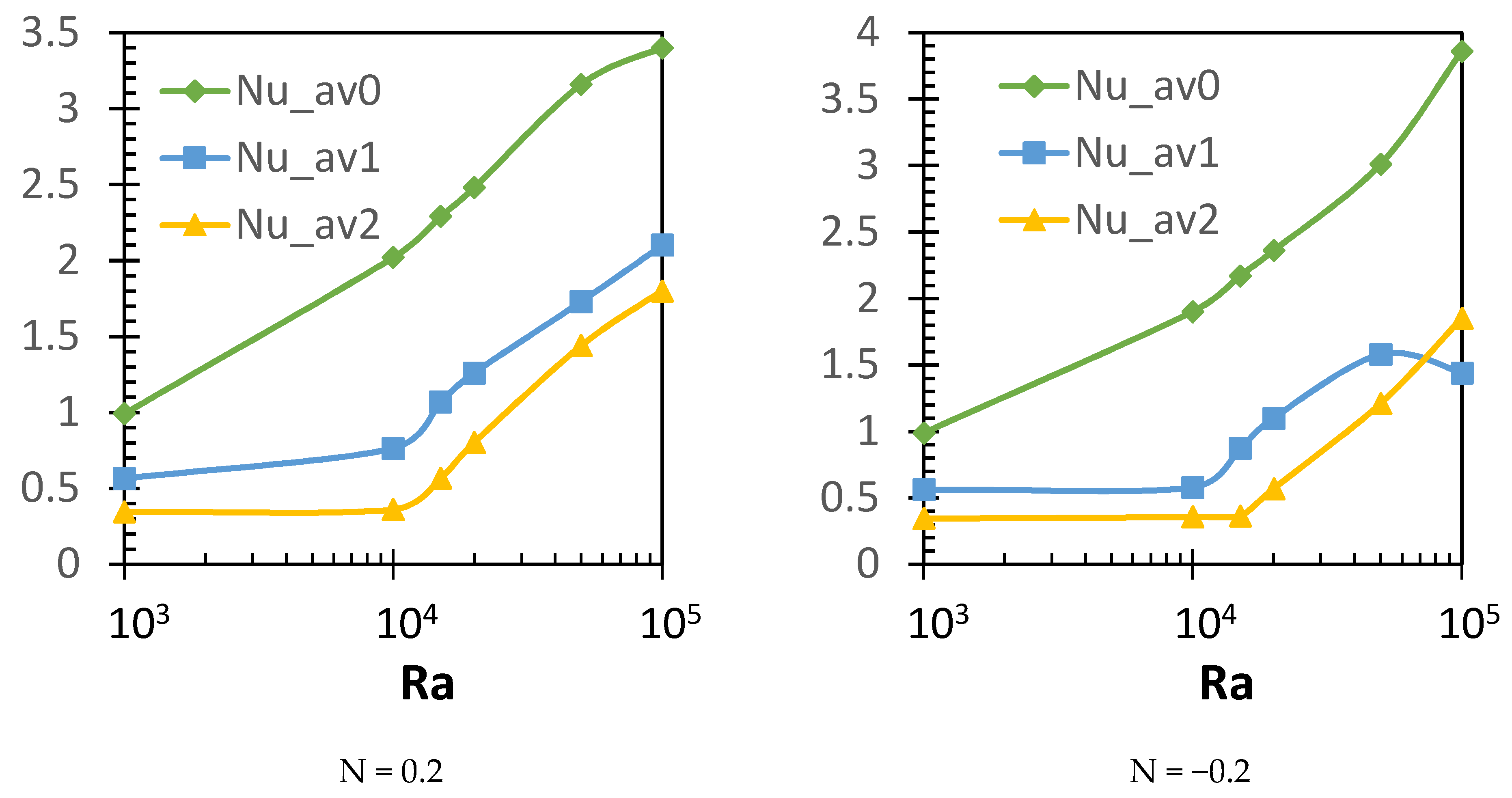
Figure 20 shows the effect of the Rayleigh number on the average heat transfer rate. The increase in Ra increases the average Nusselt number almost linearly in the reference case for both buoyancy ratio cases. For the cavity with barriers, the Ra increases from 10³ to 10⁴, and the average Nusselt is almost constant. From Ra = 10⁴, the increase in Ra, significantly increases the heat transfer ratio for both heights of the barrier studied when N = 0.2. For N = −0.2, the case of the barrier of height 1 is characterized by a maximum average Nusselt number observed at Ra = 5 × 10⁴. For the case of the barrier of height 1, the increase of the Nusselt number is observed from Ra = 1.5 × 10⁴.

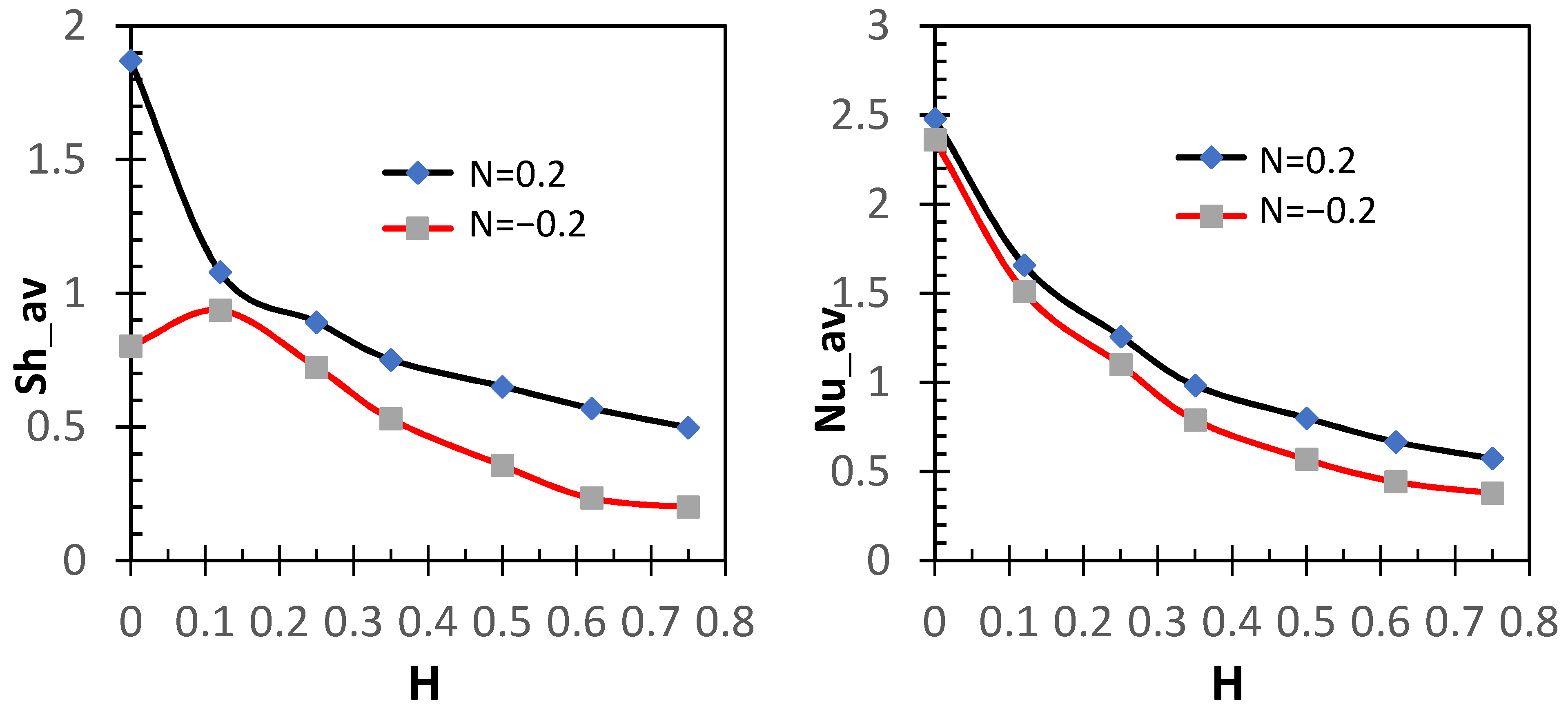
Figure 21 presents the effect of barrier height on the average mass and heat transfer ratios for Ra = 2 × 10⁴, N = 0.2 and N = −0.2. Two phases can be observed for the decrease of the average Sherwood number when N = 0.2. A decrease of 180% is detected from H = 0 to 0.12, then the curve takes a lower negative slope and the decrease is of the order of 50% from 0.12 to 0.75. When N = −0.2, there is a slight increase in the average Sherwood number from H = 0 to H = 0.12 and as the height of the barrier increases, the average mass transfer rate decreases as well.

It can also be noticed that the increase in the height of the barrier decreases the average Nusselt number. Starting from 0 to 0.35, the average Nusselt number decreases by 250%. Then by passing from H = 0.35 to 0.75, the decrease becomes about 50%.

6. Conclusions

The study presented in this paper focuses on the impact of placing an adiabatic impermeable barrier on the local dispersion of an aero-contaminant inside a three-dimensional cavity subjected to the Rayleigh–Benard conditions.

In the first part of this paper, the effect of different parameters on the dispersion of the contaminant in the case of a cavity without a barrier is analyzed. In the second part, the effect of the Rayleigh number and barrier height on the flow structure is studied through iso-concentration and iso-temperature plots for different values of N: 0, −0.2 and 0.2.

In the third part, a parametric study on the effects of the Rayleigh number, the buoyancy ratio and the barrier height on the effectiveness of the barrier in the reduction of the cavity contamination, as well as the heat and mass transfer rates, is performed.

The most important findings can be summarized as follows:

• In the absence of a barrier, the dispersion of the contaminant is mainly directed upwards at the corners of the building and to the left in the core of the building to the initially uncontaminated region, in the cases of N = 0 and N positive. Otherwise, when N is negative, the dispersal effect of the contaminant mainly occurs in a horizontal way at the bottom of the building.
• The effectiveness of the protective barrier is greater in the case of negative buoyancy ratios compared to positive values, for the same Rayleigh number and the same barrier height.
• The efficiency increases linearly with the height of the barrier.
• In the presence of the barrier, the Rayleigh number increase causes the heat and mass transfer rates to increase from Ra = 10⁴ and higher.
• The placement of the barrier strongly diminishes the heat transfer rate for all values of N. However, noticeable decrease in the mass transfer rate is only observed for positive values of N.

References

- Godish, T. Indoor Environmental Quality, 1st ed.; CRC Press: Boca Raton, FL, USA, 2000; pp. 230–250. [Google Scholar]
- Cogliano, V.J.; Grosse, Y.; Baan, R.A.; Straif, K.; Secretan, M.B.; El Ghissassi, F. Meeting Report: Summary of IARC Monographs on Formaldehyde, 2-Butoxyethanol, and 1-tert-Butoxy-2-Propanol. Enviro. Health Prespec. 2005, 113, 1205–1208. [Google Scholar] [CrossRef] [Green Version]
- Branco, P.T.B.S.; Alvim-Ferraz, M.C.M.; Martins, F.G.; Sousa, S.I.V. Children’s exposure to indoor air in urban Nurseries-Part II: Gaseous pollutants’ assessment. Environ. Res. 2015, 142, 662–670. [Google Scholar] [CrossRef] [PubMed] [Green Version]
- Little, J.C.; Hodgson, A.T.; Gadgil, A.J. Modeling emissions of volatile organic compounds from new carpets. Atmosph. Environ. 1994, 28, 227–234. [Google Scholar] [CrossRef] [Green Version]
- Yang, X.; Chen, Q.; Zhang, J.S.; Magee, R.; Zeng, J.; Shaw, C.Y. Numerical simulation of VOC emissions from dry materials. Build. Environ. 2001, 36, 1099–1107. [Google Scholar] [CrossRef]
- Guo, Z. Review of indoor emission source models. Part 1. Overview. Environ. Pollut. 2002, 120, 533–549. [Google Scholar] [CrossRef]
- Xu, Y.; Zhang, Y. An improved mass transfer-based model for analyzing VOC emissions from building materials. Atmosph. Environ. 2003, 37, 2497–2505. [Google Scholar] [CrossRef]
- Deng, B.; Kim, N. An analytical model for VOCs emission from dry building materials. Atmosph. Environ. 2004, 38, 1173–1180. [Google Scholar] [CrossRef]
- Wiglusz, R.; Sitko, E.; Nikel, G.; Jarnuszkiewicz, I.; Igielska, B. The effect of temperature on the emission of formaldehyde and volatile organic compounds (VOCs) from laminate flooring—Case study. Build. Environ. 2002, 37, 41–44. [Google Scholar] [CrossRef]
- Xiong, J.; Zhang, P.; Huang, S.; Zhang, Y. Comprehensive influence of environmental factors on the emission rate of formaldehyde and VOCs in building materials: Correlation development and exposure assessment. Environ. Res. 2016, 151, 734–741. [Google Scholar] [CrossRef] [PubMed]
- Deng, Q.H.; Zhou, J.; Mei, C.; Shen, Y.M. Fluid, heat and contaminant transport structures of laminar double-diffusive mixed convection in a two-dimensional ventilated enclosure. Int. J. Heat Mass Transf. 2004, 47, 5257–5269. [Google Scholar] [CrossRef]
- Yu-Shu, S.; Liu, D.; Wang, Y.; Zhao, F.; Li, Y. Forced flow structure and mixed convection in a ventilated porous enclosure with a local contaminant source. Int. J. Heat Mass Transf. 2019, 131, 973–983. [Google Scholar] [CrossRef]
- Zhao, F.Y.; Liu, D.; Tang, G.F. Natural convection in an enclosure with localized heating and salting from below. Int. J. Heat Mass Transf. 2008, 51, 2889–2904. [Google Scholar] [CrossRef]
- Arellano, J.S.; Gijón-Rivera, M.; Riesco-Ávila, J.M.; Elizalde-Blancas, F. Numerical study of the double diffusive convection phenomena in a closed cavity with internal CO2 point sources. Int. J. Heat Mass Transf. 2014, 71, 664–674. [Google Scholar] [CrossRef]
- Li, X.; Yan, Y.; Tu, Y.J. Effects of surface radiation on gaseous contaminants emission and dispersion in indoor environment—A numerical study. Int. J. Heat Mass Transf. 2019, 131, 854–862. [Google Scholar] [CrossRef]
- Abolhasani, M.; Abbasbandy, S.; Allahviranloo, T. A New Variational Iteration Method for a Class of Fractional Convection-Diffusion Equations in Large Domains. Mathematics 2017, 5, 26. [Google Scholar] [CrossRef] [Green Version]
- Geiser, J.; Martínez, E.; Hueso, J.L. Serial and Parallel Iterative Splitting Methods: Algorithms and Applications to Fractional Convection-Diffusion Equations. Mathematics 2020, 8, 1950. [Google Scholar] [CrossRef]
- Mallinson, G.D.; Davis, G.D.V. Three-dimensional natural convection in a box: A numerical study. J. Fluid Mech. 1977, 83, 1–31. [Google Scholar] [CrossRef]
- Wakashima, S.; Saitoh, T.S. Benchmark solutions for natural convection in a cubic cavity using the high-order time–space method. Int. J. Heat Mass Transf. 2004, 47, 853–864. [Google Scholar] [CrossRef]
- Eymard, R.; Gallouet, T.; Herbin, R. Finite Volume Methods, Handbook of Numerical Analysis; Elsevier BV: Amsterdam, The Netherlands, 2000; Volume 7, pp. 713–1020. [Google Scholar]
- Patankar, S.V. Numerical Heat Transfer and Fluid Flow, 2nd ed.; Mc Graw Hill: New York, NY, USA, 1980; pp. 25–39. [Google Scholar]
- Bejan, A. Convection Heat Transfer, 4th ed.; John Wiley: New York, NY, USA, 2013; pp. 30–289. [Google Scholar]
- Sezai, I.; Mohamad, A.A. Double diffusive convection in a cubic enclosure with opposing temperature and concentration gradients. Phys. Fluids 2000, 12, 2210–2223. [Google Scholar] [CrossRef]
- Rahmati, A.R.; Tahery, A.A. Numerical study of nanofluid natural convection in a square cavity with a hot obstacle using lattice Boltzmann method. Alexandria Eng. J. 2018, 57, 1271–1286. [Google Scholar] [CrossRef]
Figure 1.
Physical model of the building: (a) Reference model without barrier; (b) Building with barrier.
Figure 2.
Schematic view of the mesh.
Figure 3.
Comparison of the present results (bottom) of Streamlines, iso-temperature and iso-concentration with the results of Sezai and Mohamad [23] (top) at Ra = 105, Pr = 10 and Le = 10, (a): X-Y-mid-plane, (z = 0.5) and (b): Y-Z-mid-plane (x = 0.5).
Figure 4.
Particles’ trajectories, iso-concentration and iso-temperature in the building without a barrier for N = 0, Ra = 103 and 105.
Figure 5.
Particles’ trajectories of the fluid in the building for different Ra, effect of two barriers’ heights for N = 0.
Figure 6.
Contaminant iso-surfaces of concentration for different Ra, effect of two barriers’ heights for N = 0.
Figure 7.
Temperature iso-surfaces in the building for different Ra, effect of two barriers’ heights for N = 0.
Figure 8.
Particles’ trajectories of the fluid in the building for different Ra, effect of two barriers’ heights for N = −0.2.
Figure 9.
Contaminant iso-surfaces of concentration for different Ra, effect of two barriers’ heights for N = −0.2.
Figure 10.
Temperature iso-surfaces in the building for different Ra, effect of two barriers’ heights for N = −0.2.
Figure 11.
Particles’ trajectories of the fluid in the building for different Ra, effect of two barriers’ heights for N = 0.2.
Figure 12.
Contaminant iso-surfaces of concentration for different Ra, effect of two barriers’ heights for N = 0.2.
Figure 13.
Temperature iso-surfaces in the building for different Ra, effect of two barriers’ heights for N = 0.2.
Figure 14.
Iso-contours of the contaminant concentration in the building without a barrier, with the y = 0.45 plane for Ra = 2 × 10⁴ and a different buoyancy ratio.
Figure 15.
Effect of the Rayleigh number on the efficiency of the barrier for N = 0.2 and N = −0.2; Eff1 and Eff2 are the barrier efficiencies for H1 = 0.25 and H2 = 0.5, respectively.
Figure 16.
Effect of the buoyancy ratio on the efficiency of the barrier for Ra = 2 × 10⁴; Eff1 and Eff2 are the efficiencies for H1 = 0.25 and H2 = 0.5, respectively.
Figure 17.
(a) Effect of the barrier height on the efficiency for Ra = 2 × 10⁴, N = 0.2 and N = −0.2; (b) Linear trendline to efficiency variation with the barrier height; (c) Polynomial trendline to efficiency variation with the barrier height, blue color equation for N = 0.2 and red color equation for N = −0.2.
Figure 18.
Effect of the buoyancy ratio on the average heat and mass transfer ratios for Ra = 2 × 10⁴, (0): reference case, (1): H1 = 0.25 and (2) for H2 = 0.5.
Figure 19.
Effect of the Rayleigh number on the average mass transfer ratios for N = 0.2 and N = −0.2, (0): reference case, (1): H1 = 0.25 and (2) for H2 = 0.5.
Figure 20.
Effect of the Rayleigh number on the average heat transfer ratios for N = 0.2 and N = −0.2, (0): reference case, (1): H1 = 0.25 and (2) for H2 = 0.5.
Figure 21.
Effect of the barrier height on the average heat and mass transfer ratios for Ra = 2 × 10⁴, N = 0.2 and N = −0.2.