
Automatic Tempered Posterior Distributions for Bayesian Inversion Problems
by
 , , and
Luca Martino
1,* ,
,
Fernando Llorente
2,
Ernesto Curbelo
2,
Javier López-Santiago
3 and
Joaquín Míguez
3 1
Department of Signal Processing, Universidad rey Juan Carlos (URJC), 28942 Madrid, Spain
2
Department of Statistics, Universidad Carlos III de Madrid (UC3M), 28911 Madrid, Spain
3
Department of Signal Processing, Universidad Carlos III de Madrid (UC3M), 28911 Madrid, Spain
*
Author to whom correspondence should be addressed.
Mathematics 2021, 9(7), 784; https://doi.org/10.3390/math9070784
Submission received: 27 February 2021
/
Revised: 26 March 2021
/
Accepted: 1 April 2021
/
Published: 6 April 2021
(This article belongs to the Special Issue Recent Advances in Data Science)
Abstract
:We propose a novel adaptive importance sampling scheme for Bayesian inversion problems where the inference of the variables of interest and the power of the data noise are carried out using distinct (but interacting) methods. More specifically, we consider a Bayesian analysis for the variables of interest (i.e., the parameters of the model to invert), whereas we employ a maximum likelihood approach for the estimation of the noise power. The whole technique is implemented by means of an iterative procedure with alternating sampling and optimization steps. Moreover, the noise power is also used as a tempered parameter for the posterior distribution of the the variables of interest. Therefore, a sequence of tempered posterior densities is generated, where the tempered parameter is automatically selected according to the current estimate of the noise power. A complete Bayesian study over the model parameters and the scale parameter can also be performed. Numerical experiments show the benefits of the proposed approach.
1. Introduction
The estimation of unknown parameters from noisy observations is an essential problem in signal processing, statistics, and machine learning [1,2,3]. Within the Bayesian signal processing framework, these problems are addressed by constructing posterior probability distributions of the unknowns. Given the posterior, one often wants to make inference about the unknowns, e.g., if we are estimating parameters, finding the values that maximize their posterior, or the values that minimize some cost function given the uncertainty of the parameters. Unfortunately, obtaining closed-form solutions, usually expressed as integrals of the posterior, is infeasible in most practical applications. Therefore, developing approximate computational techniques, such as importance sampling and Markov chain Monte Carlo (MCMC) algorithms, is often required [4,5,6].
The so-called tempering of the posterior distributions is a well-known procedure for improving the performance of Monte Carlo (MC) algorithms [7,8,9,10]. Tempering is performed by modulating an artificial scale parameter or by sequentially including new data. There are several reasons for the improvement in performance: improving mixing, discovering modes, fostering the exploration of the inference space, etc. In the first iterations of the MC scheme, a posterior density with a bigger scale is considered. The artificial scale parameter (often called temperature) is reduced along the iterations, until considering the true posterior distribution. However, the user should select a temperature schedule, i.e., a decreasing rule for the scale parameter, which is usually chosen in an heuristic way [4,5]. In the literature, the tempering procedure has gained particular attention for the estimation of the marginal likelihood (also known as Bayesian model evidence) [9,11,12].
Furthermore, the joint inference of parameters (denoted as ) of observation models, , and scale parameters of the likelihood function (that, in the scalar case, is usually denoted as ) can be a hard task. Indeed, “wrong choices” of values can easily jeopardize the sampling of . In this work, we introduce a procedure to tackle this problem.
To be specific, in this work, we design an adaptive importance sampling (AIS) scheme [13] for Bayesian inversion problems, where an automatic tempering procedure is implemented. We assume that the vector of observations is obtained by a nonlinear transformation of the variables of interest , perturbed by additive Gaussian noise with unknown power . The nonlinear mapping usually represents a complex physical model, a computer code, etc. The resulting posterior densities are usually highly multimodal and complex distributions. Furthermore, the inference task in the joint space is particularly challenging. We introduce a split strategy to tackle this problem, involving an optimization approach over and a sampling scheme for . More specifically, we design an iterative procedure where these two tasks are alternated. Additionally, the current maximum likelihood (ML) estimate of the noise power, , is employed as a tempering parameter, starting from high values and then “cooling down” according to the ML estimates at each iteration. Therefore, the proposed scheme deals with a sequence of tempered posteriors according to the current estimation . It is important to observe that, given a fixed vector , the ML estimator can be obtained analytically.
Furthermore, the complete Bayesian analysis regarding the joint posterior of and is also possible (as discussed in Section 5). This is obtained by implementing a proper re-weighting of the samples generated by the proposed algorithm, called Automatic Tempering AIS (ATAIS), without any additional evaluations of the observation model. An approximation of the marginal posterior of is provided as well. The advantages of the proposed scheme are shown in two numerical experiments, one of them considering a complex astronomical model.
2. Problem Statement
Let us denote the observed measurements as , and the variable of interest that we wish to infer as . Furthermore, let us assume the observation model
where we have a nonlinear mapping,
and a Gaussian perturbation noise,
with , and denotes the K-dimensional identity matrix. The model can be easily extended to a matrix of observations instead of a vector, if the nonlinear mapping is of type . The noise variance is unknown, in general. The mapping may be analytically unknown: the only assumption is that we are able to evaluate it pointwise. The likelihood function is
Note that we have two types of variables of interest: the vector contains the parameters of the nonlinear mapping , whereas is a scale parameter of the likelihood function.
Given the vector of measurements , we wish to make inferences regarding the hidden parameters and the noise power , obtaining at least some point estimators and . We are also interested in performing uncertainty and correlation analysis for the components of . Furthermore, we aim to perform model selection, i.e., to compare, select, or properly average different models.
Bayesian inference in the complete space. We consider independent prior densities and over the unknowns. Therefore, the complete posterior density is
The marginal likelihood is
This quantity is often needed for model selection. While Z is generally unknown, we can usually evaluate pointwise the un-normalized posterior , i.e., . More generally, the computation of integrals of the form
where is an integrable function, is usually required. We consider a Monte Carlo quadrature approach for approximating the integral above and, more generally, provide a particle approximation of the joint posterior .
Main observation. Generating random samples from a complicated posterior in Equation (6) and efficiently computing the integrals as in Equations (7) and (8) is very often a hard task. Moreover, this task becomes more difficult when we try to perform a joint inference where scale parameters are involved, i.e., , and parameters of the nonlinearity, i.e., . Indeed, “wrong choices” of values can easily jeopardize the sampling of . In the next section, we describe a strategy that we propose to tackle this problem. Before do so, however, we need to recall some additional definitions.
Conditional and marginal posteriors. In other to design efficient computational schemes, it is often useful to consider the conditional posteriors, for instance,
In the next section, we will see that the idea underlying the proposed scheme is to split the space , restricting the sampling problem only to and considering an optimization problem with respect to . The conditional marginal likelihood is obtained by integrating out one of the two variables, e.g.,
The integral above cannot be computed analytically, in general. We can also consider marginal posteriors, for instance, the marginal posterior of is
Note that the joint posterior in Equation (6) can be also written as
Outline of the proposed approach. The underlying idea of this work is to divide the inference study in two parts. In the first part (Section 3 and Section 4), we focus on the study of the conditional posterior given a fixed . Then, in the second part (Section 5), we also estimate the marginal posterior . Finally, using (12), we can obtain a final approximation of the complete posterior . Estimations of and Z are also obtained.
3. Key Observations and Proposed Approach
3.1. Split Inference
In the first part of work, we assume a uniform proper (or improper) prior over , i.e., in . The possible use of a general choice of is discussed in Section 4.1. Let denote the MAP estimator of . Generally, should be a function of , i.e., . However, due to the choice of likelihood function (and the uniform prior) considered in this paper, we have that
which does not depend on , i.e., we have that maximizes the conditional posterior for any . See Appendix A for further details.
Furthermore, the variance of the conditional posterior grows when increases. In this sense, with larger , the density is “broader”; thus, it is easier for Monte Carlo methods to explore the space (namely, we have a tempering effect). Based on these considerations, we can run Monte Carlo schemes (specifically IS algorithms) on with a large value for estimating more efficiently. Furthermore, apart from estimating , we are also interested in studying the conditional posterior , where
The value can be obtained in closed-form (see Appendix A). In fact, for any , we have
which has the form of an Inverse Gamma density for and it has a unique mode at , where is a fixed. Therefore, finally we have
This can serve as a point estimator of the noise power in the system, and also as a threshold value to stop the tempering of the conditional posterior, as we show in the following section.
3.2. An Iterative Scheme
Consider that we start with a large value , which can be viewed as a coarse approximation of , so we denote it . Let denote an estimate of obtained by working w.r.t. . We use this current estimation to obtain the next value of , i.e., . In general, is a better estimator of than , as we have tried to evaluate of the smallest error between and the data, , i.e., , which is related to the power of the noise perturbation in the system. For instance, assuming zero noise, we would have , recalling that for . We can iterate this procedure for :
- 1
- Estimate by Monte Carlo (e.g., an IS scheme) by approximately maximizing .
- 2
- Compute
With this iterative scheme, we have that as T grows, thus we eventually perform IS with respect to the density of interest . Furthermore, a non-increasing sequence of values is produced, which facilitates the estimation of , and ensures the IS estimation of is performed efficiently by using the set of intermediate, tempered (i.e., wider) distributions for . Finally, a particle approximation of is obtained, i.e.,
where . Note that are the final corrected weights obtained at the end of the algorithm (see Algorithm 1).
4. Automatic Tempering Adaptive Importance Sampling (ATAIS)
In this section, we describe an adaptive importance sampler with an automatic tempering approach which follows the procedure given above. At each iteration t of the algorithm, we have an ML approximation of , i.e., . Considering Equation (9), we define the un-normalized tempered conditional posterior at the t-th iteration,
where we assume in . For other generic choice of , see the discussion in Section 4.1. At each iteration, we consider as the target distribution. The dependence on the iteration t occurs because varies with t. The ATAIS algorithm is outlined in Algorithm 1. The resulting scheme is an adaptive IS algorithm which combines sampling schemes and stochastic optimization. It is important to remark that if is bigger than the true ML value, we generate a non-increasing sequence of , i.e., , etc. Note that this is true as we have assumed a uniform prior . To see this, recall that . Improving means that the squared error is smaller, as shown in Equation (14), which implies that always decreases (provided that we start with ).
IS steps. A set of N samples are drawn from a (normalized) proposal density with mean and a covariance matrix . An importance weight
is assigned to each sample.
Proposal adaptation. A particle estimation of the conditional MAP estimator of is given by . The value of current MAP approximation is then compared with the value of global MAP estimator obtained so far denoted as . If , all the global MAP estimators are updated and the proposal pdf is moved at , i.e., we set
| Algorithm 1: ATAIS: AIS with automatic tempering. |
|
Otherwise, we keep the previous values of , , and . The covariance matrix is adapted by considering the empirical covariance of the weighted samples. Note that we set instead of using the empirical mean of the samples (as in other classical AIS schemes). This is because we have noticed that this choice provides better and more robust results, especially as the dimension of the problem grows.
Automatic tempering. As we showed in the previous section, the current ML estimator of can be obtained analytically as
where . If the current ML estimator is smaller than the current global one , i.e., , then we update , Otherwise, we keep the value of . Actually, with a uniform prior , every time that we update , we also update (see footnote in the previous page).
ATAIS outputs. After T iterations, a final correction of the weights is needed, i.e.,
in order to obtain a particle approximation of the measure of the final conditional posterior . Thus, the algorithm returns the final estimators , , and all the weighted samples , for all and . Other outputs can be obtained with a postprocessing of the weighted samples, as shown below. Note that Equation (22) does not require any additional evaluation of the model, and the error is . Moreover, we can also use and for building a particle approximation of any other conditional posterior . This allows the study of the marginal posterior and provides the complete Bayesian inference, as we show in the next section.
4.1. With a Generic Prior
The ATAIS algorithm is based on the fact that does not depend on . This allows us to progressively estimate it by targeting the sequence of tempered posteriors that share all the same MAP. However, in the case is not uniform, we generally have one for each , and we could have that the sequence of will not approach .
If the data are informative and the prior is chosen such it is vague with respect to the likelihood, the position of is not very sensitive to the value of . Namely, we have , and thus our algorithm can be applied in this context. When the data are not informative, we should use an even more vague prior (i.e., wider than the likelihood function) in order to maintain the usefulness of the algorithm.
5. Complete Bayesian Inference with ATAIS
Let us assume we have a proper prior and we introduce another proper prior for . The outputs of the ATAIS algorithm can serve to approximate the normalizing constant of the joint posterior , i.e., the so-called marginal likelihood or Bayesian model evidence, given by
where we have denoted , usually called conditional marginal likelihood. The quantity Z is useful for model selection purposes. Furthermore, a complete Bayesian study of the joint posterior can be provided as well.
Approximation of . After the T iterations of ATAIS, we can also approximate the conditional marginal likelihood without additional evaluations of the target function. Indeed, saving the error values at each particle obtained for the computation of the likelihood function during ATAIS,
We can compute the IS weights,
for a generic value of Thus, the IS estimator of the conditional marginal likelihood is given by the arithmetic mean of the weights ,
Approximation of Z. Drawing , for , (or considering a deterministic grid, e.g., as a Riemannian integration), we can approximate the global marginal likelihood Z by applying simple Monte Carlo to the integral in Equation (23),
Approximation of . An approximation of the marginal posterior can be also obtained as
which can be used to approximate, e.g., the MAP of by Other different moments of can be computed by a deterministic quadrature (as the problem is now one-dimensional) or applying noisy Monte Carlo approaches.
Complete Bayesian analysis. We can approximate the integral of interest as
where
and are generated by applying a noisy MCMC with invariant density . Note that the samples do not depend on the index j (they do not change) as we are recycling the particles generated by ATAIS and reusing evaluations .
6. Simulations
We test the proposed scheme in two numerical examples: The first numerical experiment is a simple bidimensional example (which is easy to be reproduced). The second experiment considers a real-world application, i.e., a radial velocity model of exoplanet systems which is often employed in astronomy applications (with a dimension of the inference problem of 6 and 11).
6.1. First Numerical Analysis
For the sake of simplicity, let us consider and an observation model given by the equation
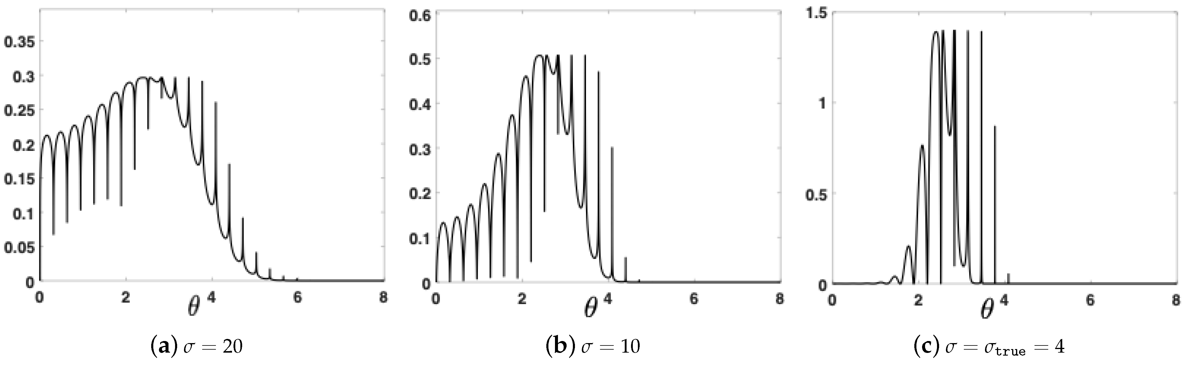
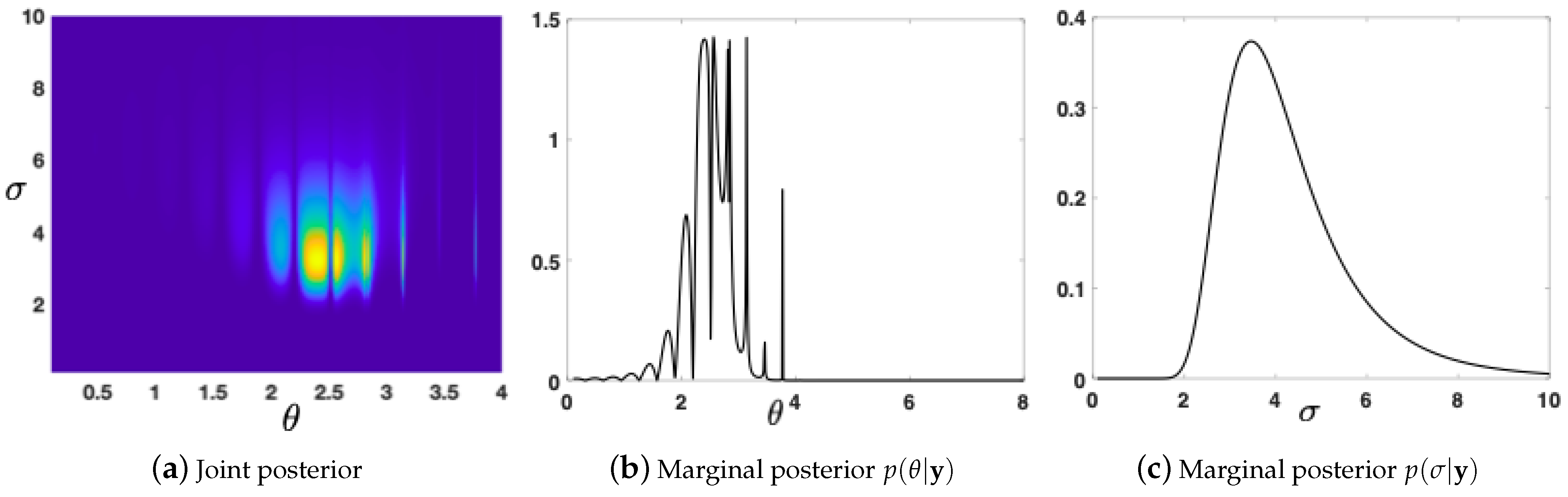
so that , and . We consider , and . We generate observations from the model above. We also consider a uniform prior for in . The conditional posterior is shown in Figure 1c. We can observe that is highly multimodal. Figure 1 also depicts the conditional posteriors with . Considering also a uniform prior over in , we have also a bidimensional joint posterior over , which is depicted in Figure 2a.
In this bidimensional example, it is possible to obtain the ground-truths using an expensive thin grid. We show the ground-truths of the different pdfs in Table 1. Moreover, the true value of the complete evidence . As the prior over is uniform, the maximum likelihood of is . The two marginal posteriors are shown in Figure 2b,c.
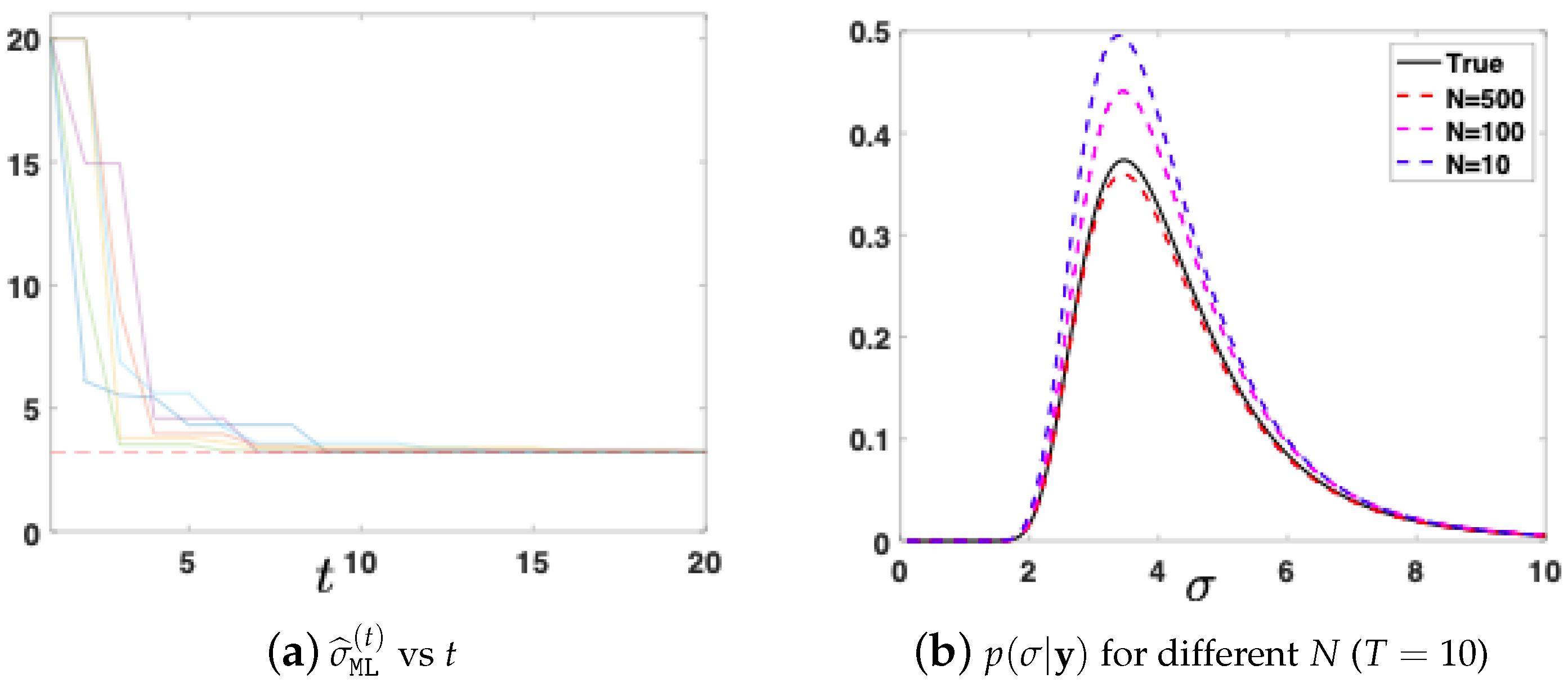
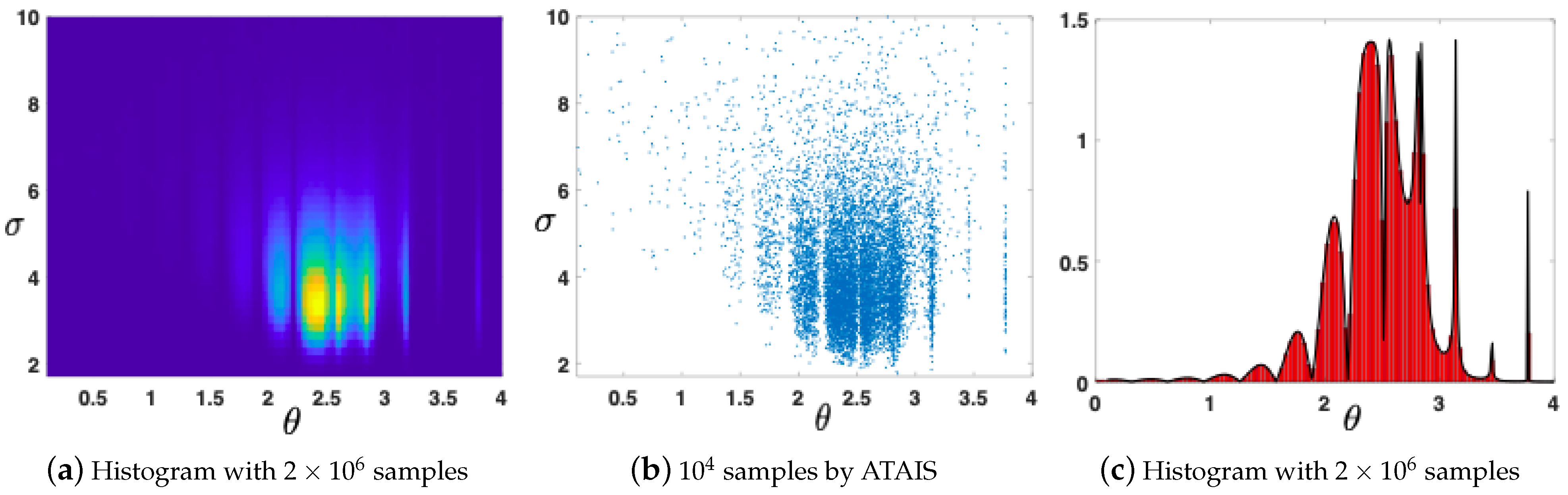
We apply ATAIS with the goal of estimating the expected value and the variance of the posterior density with respect to . We consider a Gaussian proposal with and a starting variance of . Note that is located in a region that does not contain modes. We also start with and (initial conditions). The Mean Square Error (MSE) of ATAIS, averaged over 500 runs, in estimation of different moments and modes as function of N (and with ), is given in Table 2. The ML estimation , as function of the iteration t (with ) for different runs, is given in Figure 3a. The approximation of the marginal posterior , denoted , is obtained as in Equation (27) in one specific run, with different and . The approximations of the joint posterior and the marginal posterior , obtained by resampling the particles according to the normalized weights in Equations (31) and (24), are shown in Figure 4, i.e., using a sampling importance resampling procedure. For more details, see in [14] and Chapter 24 in [15].
6.2. Radial Velocity Curves of Exoplanets and Binary Systems
In this example, we consider an application in an astronomical model. In recent years, the problem of revealing objects orbiting other stars has acquired large attention. Different techniques have been proposed to discover exo-objects but, nowadays, the radial velocity technique is still the most used [16,17,18,19]. The problem consists in fitting a model (the so-called radial velocity curve) to data acquired at different moments spanning during long time periods (up to years). The model is highly nonlinear, and it is costly in terms of computation time (especially for certain sets of parameters). Obtaining a value to compare to a single observation involves numerically integrating a differential equation in time or an iterative procedure for solving to a nonlinear equation. Typically, the iteration is performed until a threshold is reached or iterations are performed. The problem of radial velocity curve fitting is applied in several related applications.
Observation model—likelihood. When analyzing the radial velocity data of an exoplanetary system, it is commonly accepted that the wobbling of the star around the center of mass is caused by the sum of the gravitational force of each planet independently and that they do not interact with each other. Each planet follows a Keplerian orbit, and the radial velocity of the host star is given by
with and . In this equation, is the amplitude of the curve, is the argument of perigee, and is the eccentricity of the orbit of the i-th planet. The parameter represents the mean velocity, and it is common for all the planets. The number of objects in the system is S, which is considered to be known in this experiment (for the sake of simplicity). Both and depend on time t, and then is a Gaussian noise perturbation with variance . The likelihood function is defined by (32) and some indicator variables described below. The angle is the true anomaly of the planet i, and it can be determined from
This equation has analytical solution. As a result, the true anomaly can be determined from the mean anomaly M. However, the analytical solution contains a nonlinear term that needs to be determined by iterating. First, we define the mean anomaly as
where is the time of periastron passage of the planet i and is the period of its orbit. Then, through the Kepler’s equation,
where is the eccentric anomaly. Equation (35) has no analytic solution and it must be solved by an iterative procedure. A Newton–Raphson method is typically used to find the roots of this equation [20]. For certain sets of parameters, this iterative procedure can be particularly slow. We also have
The variable of interest is then the vector
Then, for a single object (e.g., a planet or a natural satellite), the dimension of is , with two objects the dimension of is etc.
This example consists in a synthetic radial velocity curve of a planetary system with one planet or two planets (i.e., or ). More specifically, we generate simulated data with a model with two planets. The orbital parameters of the planets are listed in Table 3, where P is the period of the orbit, A is the amplitude of the curve, e is the eccentricity of the orbit, is the argument of perigee, and is the last periastron passage. A mean velocity m s is assumed. A Gaussian noise perturbation is added with a standard deviation m s. To simulate observations, a total of data points are selected from three random time periods (and two planets in the system). Note that the amplitude of the radial velocity curve of the second planet is close to the noise level. We run ATAIS and a standard AIS scheme with the model with one planet and with the model with two planets. The purpose of this simulation is to check the ability of the method to detect the two planets (by approximating the model evidence).
We apply ATAIS and a standard AIS scheme [13] over the space for approximating the model evidence (marginal likelihood) of both models (one planet or two planets) with the given data (generated considering two planets). Uniform priors are considered for each parameter: , , , , and (moreover, for the standard AIS scheme). The ATAIS algorithm and the standard AIS scheme have been run with and iterations for both the model with one planet and the model with two planets. In both cases, we consider the same Gaussian proposal with a starting standard deviation of 5 for each component (note that the standard AIS scheme works in higher dimensional space due the inference over ). To decide which model is more probable, the model evidence Z of each model is estimated. More specifically, we approximate the one-planet model and the two-planet model with the ATAIS algorithm and the standard AIS scheme. When , we select the first model; otherwise, if , we select the second one. The true model is the two-planet model, as the simulated data were generated from that model. After 500 independent runs, the percentage of correct detection of the true model for ATAIS is , whereas with the standard AIS scheme is only . This is due to the difficulty of making inference jointly over . Let us denote the Bayesian factor as . In ATAIS, the expected value of the ratio between the model evidences (averaged over the 500 runs) is with a relative variance of . In the case of the standard AIS, we have and . Therefore, for ATAIS, the model with two planets is clearly more probable than the model with one planet.
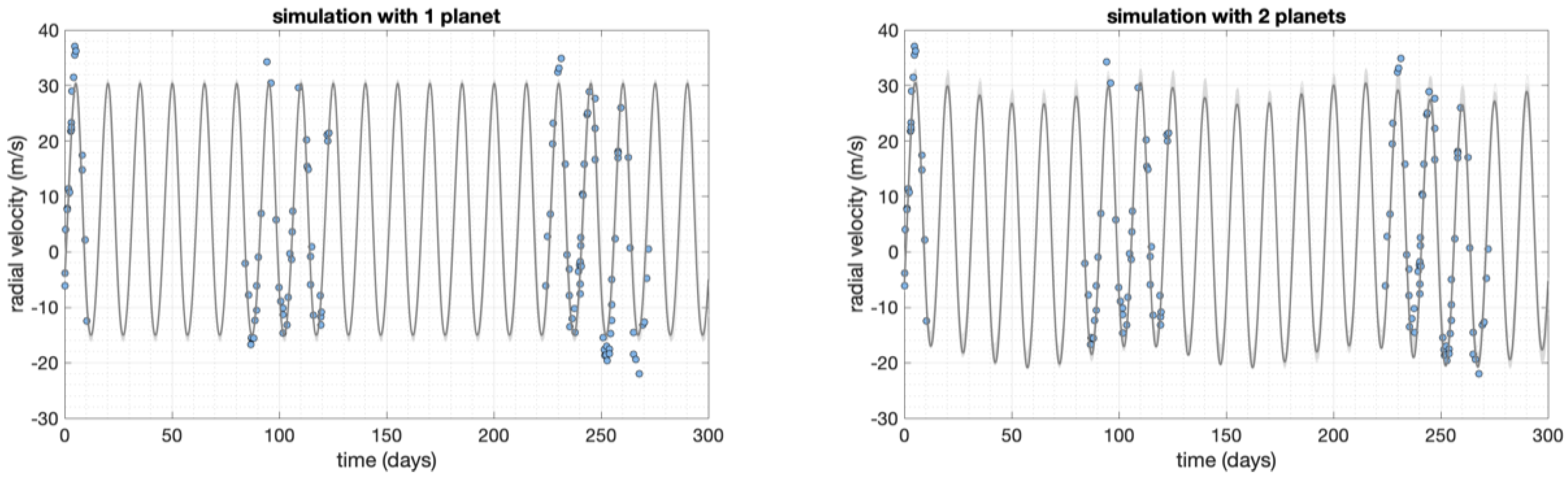
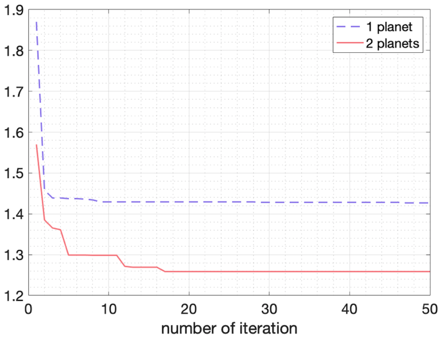
The fitted curves, corresponding to the vector of parameters obtained with ATAIS, are shown in Figure 5. From the figure, it is not clear which model better fits the simulated observations (blue points), although the model with two planets seems to better fit the observations in the time period from 200 to 300 days. The values of , obtained in one specific run by ATAIS, are given in Table 4. We notice that and are highly correlated and more iterations may be needed to obtain the actual global maximum, but the remaining parameters obtained from are similar to the simulated values. In addition, the amplitude of the curve of the second planet is close to the intensity of the noise, making it difficult to derive the best fit for that planet. Summarizing, our results show the method is able to discriminate between a model with one planet (with six dimensions of the inference problem) and a model with two planets (with 11 dimensions of the inference problem), for this particular simulation. Finally, the evolution of the automatic tempering parameter is shown in Figure 6. The dashed line is the evolution of for the single-planet model, whereas the continuous line is the evolution of for the model with two planets. In this second model, the tempering parameter reaches a smaller value, as expected.
7. Conclusions
We have proposed a novel AIS scheme for Bayesian inversion problems where an automatic tempering procedure is implemented (called ATAIS). The inference of the variables of interest and the noise power is divided. A sampling strategy is considered for and an optimization approach is employed for . Thus, ATAIS performs an iterative procedure, alternating sampling and optimization steps. Therefore, the proposed scheme deals with a sequence of tempered posteriors according to the current estimation of the noise power. We have also discussed the possibility of approximating the marginal posterior of without additional evaluations of the complex model. Furthermore, the complete Bayesian analysis regarding the complete joint posterior is possible as discussed in Section 5, again without any additional evaluations of the likelihood function.
Several simulations are provided and the application to a sophisticated astronomical model has been considered, where the number of planets in the system is detected by the analysis of the marginal likelihood. The results show the benefits of the proposed scheme. For instance, in the astronomical example, the percentage of correct detection of the true model obtained by ATAIS is ≈, whereas with the standard AIS scheme is only ≈. As future research, we plan to extend the ATAIS scheme in order to deal with an observation model with correlated noise perturbations (for instance, using a Gaussian Process). Moreover, the use of parallel AIS schemes (or MCMC algorithms) will be also considered. A combination of parallel MCMC chains and AIS schemes can be found in the so-called layered AIS method and other similar approaches [21,22]. This idea seems particularly interesting for improving the inference with radial velocity models.
Author Contributions
All the authors contribute to all the sections in the same way. All authors have read and agreed to the published version of the manuscript.
Funding
This work was partially supported by the Office of Naval Research (award no. N00014-19-1-2226), the Spanish Ministry of Science and Innovation (RTI2018-099655-B- I00 CLARA and PID2019-105032GB-I00 SPGRAPH), the Foundation by the Community of Madrid in the framework of the Multiannual Agreement with the Rey Juan Carlos University in line of action 1, Encouragement of Young Ph.D. students investigation Project under Grant F661, and the regional Government of Madrid (Comunidad de Madrid, reference Y2018/TCS-4705 PRACTICO).
Institutional Review Board Statement
Not applicable.
Informed Consent Statement
Not applicable.
Data Availability Statement
Not applicable.
Conflicts of Interest
The authors declare no conflict of interest.
Appendix A. On the Optimization of the Likelihood Function
Let us set and consider to optimize of the likelihood function
Recall that, in our model, we have . We desire to obtain
We can write the gradient and equal to zero,
We have obtained that the ML solution is defined by the system of equations,
References
- Fitzgerald, W.J. Markov chain Monte Carlo methods with applications to signal processing. Signal Process. 2001, 81, 3–18. [Google Scholar] [CrossRef]
- Andrieu, C.; de Freitas, N.; Doucet, A.; Jordan, M. An Introduction to MCMC for Machine Learning. Mach. Learn. 2003, 50, 5–43. [Google Scholar] [CrossRef] [Green Version]
- Martino, L.; Míguez, J. Generalized Rejection Sampling Schemes and Applications in Signal Processing. Signal Process. 2010, 90, 2981–2995. [Google Scholar] [CrossRef] [Green Version]
- Robert, C.P.; Casella, G. Monte Carlo Statistical Methods; Springer: New York, NY, USA, 2004. [Google Scholar]
- Liu, J.S. Monte Carlo Strategies in Scientific Computing; Springer: New York, NY, USA, 2004. [Google Scholar]
- Martino, L.; Luengo, D.; Miguez, J. Independent Random Sampling Methods; Springer: New York, NY, USA, 2018. [Google Scholar]
- Kirkpatrick, S., Jr.; Gelatt, C.D.; Vecchi, M.P. Optimization by Simulated Annealing. Science 1983, 220, 671–680. [Google Scholar] [CrossRef] [PubMed]
- Marinari, E.; Parisi, G. Simulated Tempering: A New Monte Carlo Scheme. Europhys. Lett. 1992, 19, 451–458. [Google Scholar] [CrossRef] [Green Version]
- Friel, N.; Pettitt, A.N. Marginal Likelihood Estimation via Power Posteriors. J. R. Stat. Soc. Ser. B Stat. Methodol. 2008, 70, 589–607. [Google Scholar] [CrossRef]
- Moral, P.D.; Doucet, A.; Jasra, A. Sequential Monte Carlo samplers. J. R. Stat. Soc. Ser. B Stat. Methodol. 2006, 68, 411–436. [Google Scholar] [CrossRef]
- Neal, R.M. Annealed importance sampling. Stat. Comput. 2001, 11, 125–139. [Google Scholar] [CrossRef]
- Llorente, F.; Martino, L.; Delgado, D.; Lopez-Santiago, J. Marginal likelihood computation for model selection and hypothesis testing: An extensive review. arXiv 2020, arXiv:2005.08334. [Google Scholar]
- Bugallo, M.F.; Martino, L.; Corander, J. Adaptive importance sampling in signal processing. Digit. Signal Process. 2015, 47, 36–49. [Google Scholar] [CrossRef] [Green Version]
- Rubin, D.B. Using the SIR algorithm to simulate posterior distributions. In Bayesian Statistics 3, Ads Bernardo, Degroot, Lindley, and Smith; Oxford University Press: Oxford, UK, 1988. [Google Scholar]
- Gelman, A.; Meng, X.L. Applied Bayesian Modeling and Causal Inference from Incomplete-Data Perspectives; John Wiley & Sons: New York, NY, USA, 2018. [Google Scholar]
- Gregory, P.C. Bayesian re-analysis of the Gliese 581 exoplanet system. Mon. Not. R. Astron. Soc. 2011, 415, 2523–2545. [Google Scholar] [CrossRef] [Green Version]
- Barros, S.C.C.; Brown, D.J.A.; Hébrard, G.; Gómez Maqueo Chew, Y.; Anderson, D.R.; Boumis, P.; Delrez, L.; Hay, K.L.; Lam, K.W.F.; Llama, J.; et al. WASP-113b and WASP-114b, two inflated hot Jupiters with contrasting densities. Astron. Astrophys. 2016, 593, A113. [Google Scholar] [CrossRef]
- Affer, L.; Damasso, M.; Micela, G.; Poretti, E.; Scand ariato, G.; Maldonado, J.; Lanza, A.F.; Covino, E.; Garrido Rubio, A.; González Hernández, J.I.; et al. HADES RV program with HARPS-N at the TNG. IX. A super-Earth around the M dwarf Gl 686. Astron. Astrophys. 2019, 622, A193. [Google Scholar] [CrossRef] [Green Version]
- Trifonov, T.; Stock, S.; Henning, T.; Reffert, S.; Kürster, M.; Lee, M.H.; Bitsch, B.; Butler, R.P.; Vogt, S.S. Two Jovian Planets around the Giant Star HD 202696: A Growing Population of Packed Massive Planetary Pairs around Massive Stars? Astron. J. 2019, 157, 93. [Google Scholar] [CrossRef] [Green Version]
- Press, W.H.; Teukolsky, S.A.; Vetterling, W.T.; Flannery, B.P. Numerical Recipes in C++: The Art of Scientific Computing; Springer: New York, NY, USA, 2002. [Google Scholar]
- Martino, L.; Elvira, V.; Luengo, D.; Corander, J. Layered Adaptive Importance Sampling. Stat. Comput. 2017, 27, 599–623. [Google Scholar] [CrossRef] [Green Version]
- Botev, Z.I.; Ecuyer, P.L.; Tuffin, B. Markov chain importance sampling with applications to rare event probability estimation. Stat. Comput. 2013, 23, 271–285. [Google Scholar] [CrossRef]
Figure 1.
Conditional posteriors corresponding to different values of : (a) , (b) , and (c) .

Figure 2.
The bidimensional joint posterior and the two marginal posteriors , in Equation (11), computed by using a thin grid approximation.
Figure 2.
The bidimensional joint posterior and the two marginal posteriors , in Equation (11), computed by using a thin grid approximation.

Figure 3.
(a) The maximum likelihood (ML) estimation (different runs) versus the number of iterations t, with . (b) The true marginal posterior and different approximations, in one specific run, obtained as in Equation (27) with different and (thus, the total number of samples are ).
Figure 3.
(a) The maximum likelihood (ML) estimation (different runs) versus the number of iterations t, with . (b) The true marginal posterior and different approximations, in one specific run, obtained as in Equation (27) with different and (thus, the total number of samples are ).

Figure 4.
Approximations obtained with ATAIS. (a,b) Joint posterior : (a) by an histogram with samples; (b) samples from joint posterior obtained by ATAIS. (c) Approximation by an histogram with samples, of the marginal posterior .
Figure 4.
Approximations obtained with ATAIS. (a,b) Joint posterior : (a) by an histogram with samples; (b) samples from joint posterior obtained by ATAIS. (c) Approximation by an histogram with samples, of the marginal posterior .

Figure 5.
Comparison of the results of the ATAIS algorithm with the simulations (blue dots). Left panel shows, in gray, the radial velocity curve for using a model with one planet. Right panel is like left panel but considering a model with two planets.
Figure 5.
Comparison of the results of the ATAIS algorithm with the simulations (blue dots). Left panel shows, in gray, the radial velocity curve for using a model with one planet. Right panel is like left panel but considering a model with two planets.

Figure 6.
Evolution of the tempering parameter . We decide as starting value (the figure shows from ), which is an arbitrary high value to help the exploration in the first iteration. However, after the first iteration, the algorithm is able to obtain reasonable values of . The dashed line is the evolution for the model with one planet. The continuous line is the evolution of the two-planet model.


Table 1.
Summary of pdfs and ground-truths for the first numerical experiment.
| Expectation | Variance | MAP | |
|---|---|---|---|
| 2.48 | 0.11 | 2.56 | |
| 4.32 | 2.43 | 3.46 | |
| 2.46 | 0.18 | 2.56 |
Table 2.
Mean Square Error (MSE) of ATAIS (averaged over 500 runs), in the estimation of the evidence, different moments and modes as function of N and .
Table 2.
Mean Square Error (MSE) of ATAIS (averaged over 500 runs), in the estimation of the evidence, different moments and modes as function of N and .
| Value | Ground-Truths | ||||
|---|---|---|---|---|---|
| 0.0311 | 0.0098 | 0.0034 | 0.0024 | 2.48 | |
| 0.0474 | 0.0370 | 0.0298 | 0.0201 | 0.11 | |
| 0.0410 | 0.0337 | 0.0285 | 0.0127 | 2.56 | |
| 0.9233 | 0.0785 | 0.0097 | 0.0023 | 4.32 | |
| 6.1869 | 0.2640 | 0.0035 | 0.0010 | 2.43 | |
| 0.0056 | 0.0004 | 0.0001 | 3.46 | ||
| 3.23 | |||||
Table 3.
Main orbital parameters of the two exoplanets in the simulation.
| Parameter | Planet 1 | Planet 2 |
|---|---|---|
| P | 15 d | 115 d |
| A | 25 m s | 5 m s |
| e | 0.1 | 0.0 |
| 0.61 rad | 0.17 rad | |
| 3 d | 24 d |
Table 4.
The value of and the variances of the marginal posteriors for the 2-planets model (with data points).
Table 4.
The value of and the variances of the marginal posteriors for the 2-planets model (with data points).
| Parameter | Planet 1 | Planet 2 | ||
|---|---|---|---|---|
| —Planet 2 | ||||
| P | 14.99 d | 0.18 | 110.39 d | 11.28 |
| K | 23.78 m s | 0.52 | 3.50 m s | 0.44 |
| e | 0.05 | 0.047 | 0.00 | 0.003 |
| 7.69 rad | 0.61 | 0.68 rad | 0.82 | |
| 6.8 d | 0.76 | 7.96 d | 20.31 | |
Publisher’s Note: MDPI stays neutral with regard to jurisdictional claims in published maps and institutional affiliations. |
© 2021 by the authors. Licensee MDPI, Basel, Switzerland. This article is an open access article distributed under the terms and conditions of the Creative Commons Attribution (CC BY) license (https://creativecommons.org/licenses/by/4.0/).
Share and Cite
MDPI and ACS Style
Martino, L.; Llorente, F.; Curbelo, E.; López-Santiago, J.; Míguez, J. Automatic Tempered Posterior Distributions for Bayesian Inversion Problems. Mathematics 2021, 9, 784. https://doi.org/10.3390/math9070784
AMA Style
Martino L, Llorente F, Curbelo E, López-Santiago J, Míguez J. Automatic Tempered Posterior Distributions for Bayesian Inversion Problems. Mathematics. 2021; 9(7):784. https://doi.org/10.3390/math9070784
Chicago/Turabian StyleMartino, Luca, Fernando Llorente, Ernesto Curbelo, Javier López-Santiago, and Joaquín Míguez. 2021. "Automatic Tempered Posterior Distributions for Bayesian Inversion Problems" Mathematics 9, no. 7: 784. https://doi.org/10.3390/math9070784
Note that from the first issue of 2016, this journal uses article numbers instead of page numbers. See further details here.