Diving Deep into Short-Term Electricity Load Forecasting: Comparative Analysis and a Novel Framework

Abstract

In this article, we present an in-depth comparative analysis of the conventional and sequential learning algorithms for electricity load forecasting and optimally select the most appropriate algorithm for energy consumption prediction (ECP). ECP reduces the misusage and wastage of energy using mathematical modeling and supervised learning algorithms. However, the existing ECP research lacks comparative analysis of various algorithms to reach the optimal model with real-world implementation potentials and convincingly reduced error rates. Furthermore, these methods are less friendly towards the energy management chain between the smart grids and residential buildings, with limited contributions in saving energy resources and maintaining an appropriate equilibrium between energy producers and consumers. Considering these limitations, we dive deep into load forecasting methods, analyze their performance, and finally, present a novel three-tier framework for ECP. The first tier applies data preprocessing for its refinement and organization, prior to the actual training, facilitating its effective output generation. The second tier is the learning process, employing ensemble learning algorithms (ELAs) and sequential learning techniques to train over energy consumption data. In the third tier, we obtain the final ECP model and evaluate our method; we visualize the data for energy data analysts. We experimentally prove that deep sequential learning models are dominant over mathematical modeling techniques and its several invariants by utilizing available residential electricity consumption data to reach an optimal proposed model with smallest mean square error (MSE) of value 0.1661 and root mean square error (RMSE) of value 0.4075 against the recent rivals.

1. Introduction

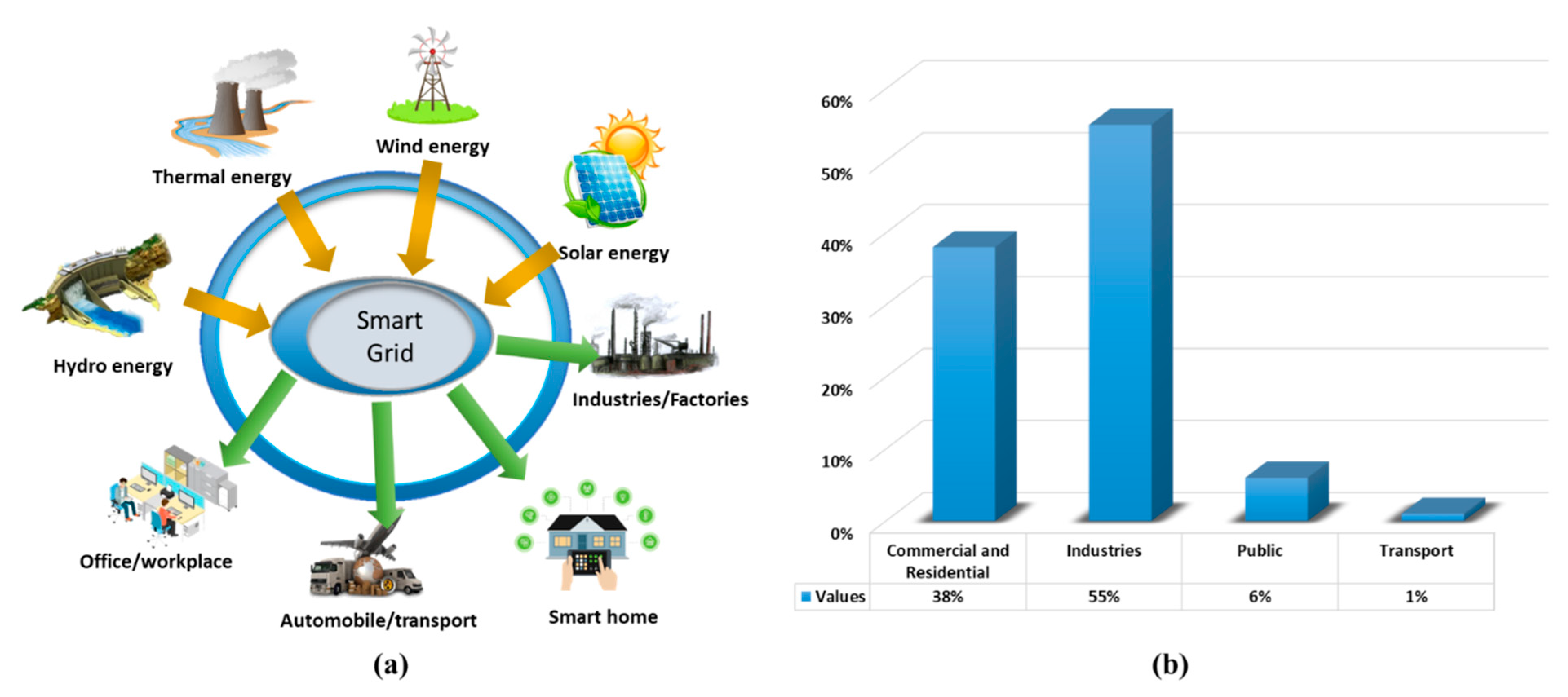
In recent decades, the consumption of energy in different sectors such as industries, factories, transportation, and residential buildings, has tremendously increased due to over population and economy growth. About 39% of total global energy is consumed by buildings and 38% is dissipated in CO₂ emissions [1]. Examining this, we need to reduce the extra energy consumption in buildings to protect and preserve energy for more efficient usage [2]. Therefore, predictions of future energy usage have encouraged several researchers to boost smart grids’ performance, that directly affect the energy production and consumption. Predictions of energy usage ensure that proper plans are available to meet the energy demands of certain buildings and control energy distribution in ways that add extra benefits to the setup of smart grids. Similarly, intelligent buildings’ profiling plays a vital role in making decisions for energy conservation and its management [3,4]. It assists users by providing insights about energy consumption behavior, that residential owners can use for certain building operations relating energy usage and helps design proper infrastructure [5]. Similarly, intelligent buildings profiling helps to detect outliers in consumption and to perceive any risks in advance [6], which is helpful because energy demand is greatly affected by inhabitant’s behavior when using household electronic devices. Considering this, the authorities operating smart grids are developing new algorithms to handle the consumption of energy in efficient ways. Since home appliances are normally used without proper forms of energy management, a lot of energy is being wasted. Reducing this wastage is very important to preserve as much energy as possible for future usage through efficient prediction techniques. Energy usage and its management infrastructure vary from building to building and similarly in industrial zones worldwide. The smart grid acts as a hub to cover both the transmission and distribution of energy. A thorough overview of production and distribution scenario of a functional smart grid is given in Figure 1a. The energy production resources include thermal, solar, wind, etc.

Similar to a number of production resources, energy is also consumed at varied points and locations, depending upon the application under consideration. For instance, as given in Figure 1b, energy consumption in South Korea is highlighted, that is distributed among industries, residential buildings, transportation, etc. [7]. Statistical analysis [8] suggests that the energy consumed by residential and commercial buildings, public, industries, and transportation in South Korea is 38%, 6%, 55%, and 1% of total energy consumption, respectively, as is shown in Figure 1b.

Analyzing the historical data from these varied consumption resources i.e., residential buildings and industries assists in planning future energy production and its efficient consumption. Maintaining a sufficient amount of energy supply has a vital role in human welfare, while the energy production resources tends to maintain and continuously improve their distribution services. The recorded amount of energy distributed in a certain time and varied weather conditions assists to predict the future energy consumption. From time-series analysis perspective, the energy patterns recorded in varied scenarios are either fed to a mathematical model or a machine learning model for energy forecasting. Several energy forecasting methods are used to estimate the future energy demand.

The existing energy forecasting literature has a lot of contributions from researchers to effectively analyze the time-series data produced by smart meters. But studies reveal that the majority of the methods model various features such as weather prediction, product price, household expenses, and their relationship through statistical methods. These features allow the changes to be explained and the cost to be estimated relatively easy. However, as shown in the energy domain and its related literature, the research attention widely increased with the practice of deep learning and sequential time-series methods. These methods have shown a tremendous performance in many data science applications, including energy forecasting domain. Although, the usage of deep learning in energy forecasting boosted the preciseness of current models, but existing literature has rarely focused on household energy management. Regarding energy management and forecasting problems, ensemble learning and its invariants has remained unexplored for residential energy consumption data. Moreover, the literature on deep sequential learning, such as recurrent neural networks (RNNs), reveal its reasonable outputs to deal with different tasks and achieve superiority. However, its several variants are the missing pieces of residential energy management. With the aforementioned assumptions in mind, this article presents a novel three-tier framework for energy consumption prediction (ECP). The notable contributions of the proposed method are given below:

• The data obtained via smart sensors and meters have several abnormalities, uncertainties, and outliers that occur due to weather variations, government influences, etc. To handle this issue, we employ a preprocessing step that includes data cleansing, its organization, noise removal, normalization, and arrange it in rolling windows to obtain the refined data, so that it is the best fit for the next training step.
• To deeply evaluate and consider mathematical modeling in the ECP domain, we apply several ELAs in this research and compared their performances with several deep sequential learning methods to learn about their effectiveness and real-world implementation potentials.
• The literature on sequential learning, such as recurrent neural networks (RNNs), shows promising outcomes for several tasks, improving on traditional learning methods. Inspired from this, we employ an RNN and its several variants such as long short-term memory (LSTM), bidirectional LSTM (Bi-LSTM), and multilayer LSTM (M-LSTM). These variants are more suitable for ECP of residential buildings.
• We experimentally prove that the sequential learning models are the most appropriate algorithms to handle the energy forecasting problem, verified by the lowest error rates using publicly available data.

The reminder of the paper is organized as follows: Section 2 covers the literature review and Section 3 provides the three-tier method for ECP, while Section 4 discuss the experimental results. Section 5 concludes the proposed method with some future directions.

2. Literature Review

Due to the widespread usage of ECP applications across the world, it has gained a considerable research attention. Several techniques have produced realistic and promising results to manage energy consumption. To thoroughly overview the existing methods, we divide them into conventional and deep learning-based methods.

2.1. Conventional Energy Management

In the initial stages, statistical methods were broadly used by the researchers. For instance, Zhong et al. [9] proposed a support vector machine (SVR)-based method for ECPs where the multidistortion generated the optimal features space in the data. They approximated a high nonlinearity between the input and output through linearity. Next, Guo et al. [10] introduced a machine learning-based model to predict the response time of a building’s thermal energy. They considered multiple linear regression (MLR), support vector machine (SVM), and extreme learning machine model for energy prediction. They analyzed the performance of each model for heating analysis. Similarly, Liu et al. [11] analyzed SVM for ECPs in the buildings. Zhang et al. [12] explored the SVM model to predict the energy consumption in the iron making process. Further, they considered a particle swarm algorithm to improve the consumption prediction. Cauwer et al. [13] detected and quantified the correlation between the energy consumption and the kinematics parameters. They considered the vehicle dynamics as the underlined physical model and used MLR for the construction of three other models. The authors formed a distant level of aggregations used by the models to allow predictions via different types of input parameters. Cai et al. [14] classified the consumption ratings of 16,000 residential houses based on the data collected from the whole region. They shortened the electric patterns using data mining approaches and used the K-mean algorithm to accomplish clustering, where the electricity usage was distributed through the obtained centers of each cluster and then SVM was used for classification. Moreover, Fumo et al. [15] established a simple, multiple, and quadratic regression for hourly and daily energy consumption in residential buildings.

Data quality is an important issue to consider in the forecasting problem and has a high impact on the forecasting algorithm. For instance, Luo et al. [16] investigated the integrity of data over the load forecasting problem. For this purpose, they considered several regression models and simulated a few data integrity attacks to identify their effects on the model’s performance. They demonstrated that the existing regression methods failed to give reasonable forecasting results. Similarly, Zhang et al. [17] studied the impact of data attacks over the accuracy of forecasting models. In their method, they verified that the most robust and representative power forecasting models are SVM and K-nearest neighbors (KNNs) combined with kernel density.

2.2. Deep Learning-Based Energy Management

Nowadays, research communities use deep learning methods due to their reasonable results in solving different energy and computer vision related applications such as energy systems [18]. Recently, He et al. [19] proposed a deep learning algorithm-based data driven approach in an unsupervised learning manner to extract the sensitive consumption features from the machinery data and developed a prediction model in a supervised manner. Similarly, Hu et al. [20] developed the stacked hierarchy of reservoirs (DeepESN) to predict the energy consumption and wind power generation through a deep learning framework. DeepESN combined the time-series ability of the state network and learning ability of the framework. Further, Ullah et al. [21] presented a clustering-based analysis of energy consumption and categorized the usage of electricity. Similarly, Gao et al. [22] proposed deep learning models such as a sequence to sequence model and two-dimensional convolutional neural network (CNN). They used a transfer learning approach to empower the prediction accuracy obtained for residential buildings. In addition, the sequential learning techniques have also been considered for the forecasting problem. For instance, Somu et al. [23] presented eDemand, which is an energy consumption model that employs LSTM. They improved the sine and cosine optimization algorithms for building energy forecasting. In this regard, Hussain et al. [24] enveloped the energy forecasting methods into one platform that covers both the deep learning and conventional methods. They also provided a statistical analysis of the energy forecasting methods. Furthermore, Li et al. [25] proposed an evolutionary algorithm known as teaching–learning-based optimization (TLBO) for short-term energy consumption in residential buildings. They further improved the prediction process using an artificial neural network where the CNN layers are capable of extracting spatial and temporal features from the data sequence. Recently, Ullah et al. [26] proposed a method where the CNN is combined with multilayer bidirectional LSTM for energy consumption of a household. Inspired by LSTM, Wen et al. [27] used a deep RNN along with LSTM for power load and photovoltaic power forecasting in the microgrid. They proved that the deep RNN with LSTM performed very well compared to multilayer perceptron. They optimized the load dispatch by particle swarm optimization PCO.

3. Material and Method for ECP

In this section, we discuss each step of our method in a detailed fashion. We discuss the ESA and sequential learning methods for ECP with the coverage of the statistical methods. The load data considered are from the household and are used to evaluate the effectiveness of the proposed method.

3.1. Data Setting and Preprocessing

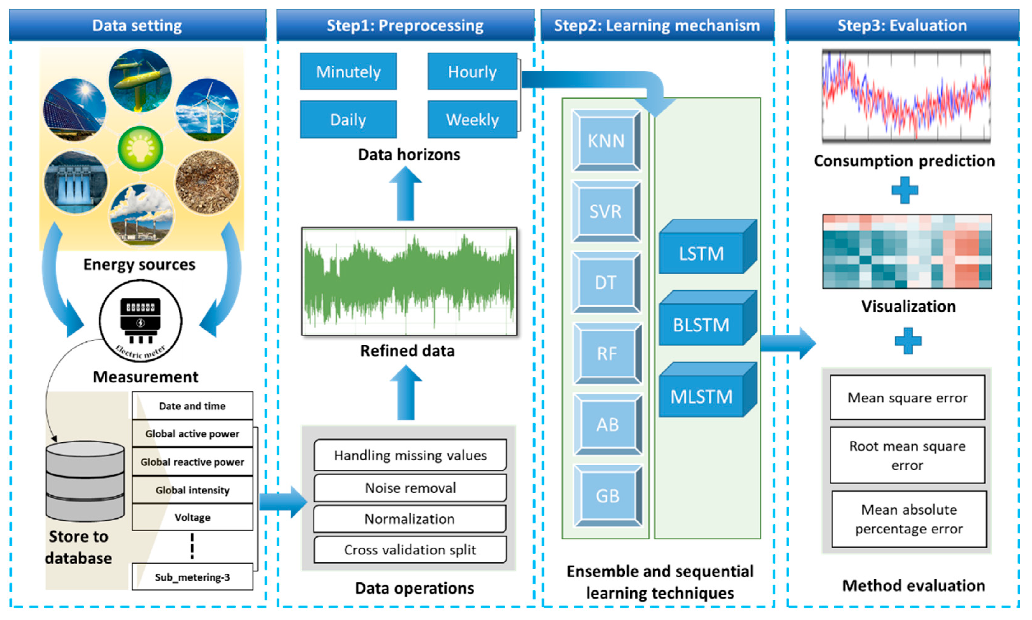
In this section, we discuss the data setting and how it is preprocessed. Usually, during a data collection process, the smart meters are connected to the main board that measures the power, current, voltage, etc., of all the appliances installed inside the house. However, there is somehow uncertainty in the data, which is one of the big problems and drastically affects the ECP. These uncertainties in the data are emerged due to different environmental conditions such as the occupant’s behavior, building’s infrastructure, noisy values generated by the system software during its settings, etc. The uncertainties in the case of ECPs include outliers, and missing values, verifying its negative affect in the final prediction results. However, energy forecasting is one of the critical steps in efficient energy management to smartly utilize the energy that balances the smart grids and the residential buildings. Prediction of energy consumption in the short term has been studied extensively, while the forecasting is less explored when going deeper at the aggregate level. The uncertainty increases as the samples size becomes smaller. Several methods [28,29] have widely focused on the difficulties and uncertainties that arise when dealing with the consumption prediction problem. Consequently, the proposed method is evaluated by the publicly available benchmarks such as power consumption dataset. Hence, this dataset contains missing values and noisy values. The initial data contain outliers and uncertainties that lead the system to an incorrect prediction of energy consumption. To deal with these uncertainties, the data are first passed through preprocessing layer that applies smoothing filters to make the data perfect for the actual modeling. The missing values are substituted by the previous values. Furthermore, there were some data outliers that were replaced through the normalization technique which brought all the values into same range to help in the smooth processing of the data. Once the data are refined and ready for processing, different horizons are formed from the data, such as minutes, hours, days, and weeks, for detailed investigation. This step is visually shown in Figure 2 as step 1 and step 2.

3.2. Learning Mechanism

We applied several ELAs to evaluate their performances for ECPs. Similarly, we used the most popular deep sequential learning techniques that are abundantly used due to their promising results, as given below.

3.2.1. ELA

In this section, we discuss several ELAs to assess their effectiveness and performance for ECP. The ELAs blend multiple predictor forecasting techniques to increase the generalization and robustness. These algorithms can be categorized into (1) the average algorithm, that considers several independent predictors to average forecasts such as those from bagging methods or the random forest (RF) method, while (2) boosting algorithms combine several low-level techniques to make a powerful performance ensemble such as Adaboost (AB) and gradient boosting. In order to perform the short-term consumption prediction, the actual power is considered from the energy data. Furthermore, a detailed explanation is given below.

AB Algorithm

AB is the most popular machine learning algorithm that is introduced by Freund et al. [30] and was originally based on the task of classification. The core concept of this algorithm is to repeatedly fit the sequence from the weak learners by modifying the data. The modification in the data is brought about through change in the weights for each classifier. Firstly, all the weights are distributed equally and for each iteration, the algorithm updates its weights. The weights are updated for those classifiers which wrongly predict the data sequence. This algorithm is adaptive in the case when its subsequent weak learners are tweaked in the favor of instances that are wrongly predicted by the previous classifier. AB obtains the input as a training set (X₁, Y₁), …, (x_m, y_m), where x_i belongs to a certain domain space while each y_i is a label in set Y. AB continuously calls the base algorithms a series of N = 1, …, N. The core idea of this algorithm is maintenance of distribution or weights in the training set. Consequently, there is another flavor of ensemble algorithm, ABR2 [31], which is the modified version of regression for the AB ensemble [30]. This algorithm sequentially fits the estimators, where each estimator focuses on the samples that were predicted by the high loss. The core features of AB R2 are the dataset and the sampling distribution. Each training data element contains a value in sampling distribution which shows the probability of the included element in the training set. The detailed pseudocode of AB is given in

Table 1. Mathematical step-by-step explanation of the working flow of the ensemble learning algorithm (ELA) representing Adaboost (AB) [32].

AB 1 ELA

Input: ($x_1,y_1)$,….($x_m,y_m$) where $x\_iϵX,y\_iϵY=\left\{-1,+1\right\}$) Initialize $〖\mathcal{D}〗\_1\left(i\right)=\frac{1}{m}$ For n = 1,….,N:    Train weak learner using ${\mathcal{D}}_n$.    Obtain weak hypothesis $h_n$: X→ {−1, +1} with error            ${ϵ}_n$= $P{r}_{i~{\mathcal{D}}_n}\left[h_n\left(x_i\right)\ne y_i\right]$.    Select ${\alpha }_n$=$\frac{1}{2}\ln \left(\frac{1-{ϵ}_n}{{ϵ}_n}\right)$    Update:       ${\mathcal{D}}_{t+1}\left(i\right)$ = $\frac{{\mathcal{D}}_t\left(i\right)}{Z_i}$×$\{\begin{array}{c}{e}^{-a_t} if h_t\left(x_i\right)=y_i \\ e^{-a_t} if h_t\left(y_i\right)\ne y_i\end{array}$          =$\frac{{\mathcal{D}}_i\exp \left(-{\alpha }_n{y}_i{h}_t\left(a_i\right)\right)}{Z_t}$    Here, $Z_t$ represents factor of normalization Output: final hypothesis:                       $H\left(a\right)$ = sign (${\sum }_{n=1}^N{\alpha }_n{h}_t\left(a\right)$)

while the pseudocode for ABR2 is given in

Table 2. Mathematical step-by-step explanation of the working flow of ELA representing ABR2 [33].

AB2 ELA

Input: Dataset D: ($x_1,y_1)$,….($x_m,y_m$) Initialize $S_1$ [i]=$\frac{1}{m}$ for all i; make n = 1 Construct Training-set from D using $S_1$. Develop network $h_n$ and train using Training-set Find max loss, $L_{max}$, over Dataset where: $L_{max}=\sup \left|h_n\left(x_t\right)\right|$ over i Calculate loss for each sample in Dataset by: $L_t$=$\frac{\left|h_n\left(x_n\right)-{\mathrm{y}}_n\right|}{L_{max}}$ Calculate weighted loss: $L^{-}={\sum }_i^n{L}_n{\mathcal{D}}_n\left(i\right)$ Set: ${\beta }_n$= $L^{-}$/(1 − $L^{-}$) Calculate next distribution: ${\mathcal{D}}_{n+1}$(i) = $\frac{{\mathcal{D}}_n\left(i\right){\beta }_n^{1-L_n}}{Z_n}$ Where $Z_n$ shows normalization factor selected so that ${\sum }_n{\mathcal{D}}_{n+1}$ sums to 1. n = n + 1; repeat 2-8 till $L$ < 0.5.

.

GBR Algorithm

The gradient boosting regression (GBR) algorithm was originally developed for regression and classification problems. This algorithm produces a prediction model in an ensemble of weak prediction models, such as the decision tree (DT) model. Next, it builds the model stage-wise as other conventional boosting techniques. It generalizes the method through the optimization of differentiable loss. This algorithm considers the low performance method of DTs to develop the prediction model on the basis of the ensemble algorithm. GBR sequentially keeps the model updated and uses the optimization of loss function to reach its generalization.

GBR sequentially keeps the model updated and uses the optimization of loss function to achieve generalization. This algorithm considers the additive model from the formula [34] given in Equation (1), where $hm\left(x\right)$ represents the main functions that are known as weak learners in the boosting context, while $\gamma m$ is the length that is chosen while executing the function given in Equation (2).

$$F\left(x\right)= {\displaystyle \sum }_{m=1}^M\gamma mhm\left(x\right)$$

(1)

$$\gamma m= argmi{n}_y{\displaystyle \sum }_{i=1}^{n}L(yi, F_m\left(xi\right)-y\frac{\theta L\left(yi, F_m-1\left(xi\right)\right)}{\theta F_m-1\left(xi\right)})$$

(2)

$$F_m\left(x\right)= F_m-1\left(x\right)+ \gamma mhm\left(x\right)$$

(3)

$$F_m\left(x\right)= F_m-1\left(x\right)+ argmi{n}_h{{\displaystyle \sum }}_{i=1}^{n}L\left(yi, F_m-1\left(xi\right)-h\left(x\right)\right)$$

(4)

Consequently, as like other boosting algorithms, GBR has the capability to create the additive model within forward stage, which is illustrated in Equation (3). At every stage, $hm\left(x\right)$ is used to minimize the loss function L in the model $F_m-1$ and fit $F_m-1$(xi), which is shown in Equation (4). The GBR model is implemented in python with the scikit-learn library. The total number of estimators used is 50. The depth of the independent regression predictors is tuned. The pseudocode of GBR is given in

Table 3. Mathematical step-by-step explanation of the working flow of ELA representing gradient boosting regression (GBR) [35].

GBR

Inputs: ▪ input sample ${\left(x,y\right)}_{i=1}^N$ ▪ iteration $I_n$ ▪ loss function $\psi$(y, f) ▪ base-learner model L(a, $\theta$) Steps: (1) initialize $f_0$ using a constant (2) for n = 1to $I_n$ do (3)   find negative gradient $g_n$($x$) (4)   fit base learner function $L\left(x,{\theta }_n\right)$ (5)   compute best gradient descent step-size ${\rho }_n$:   ${\rho }_n=argmi{n}_{\rho }{\sum }_{i=1}^N\psi \left[b_i,f_{n-1}\left(x_i\right)+\rho L\left(x_i,{\theta }_n\right)\right]$ (6) Update function: $f_n$←$f_{n-1}+$${\rho }_{n}L\left(x,{\theta }_n\right)$ end for

.

RF Algorithm

RF is also an ensemble learning method that is developed for regression and classification problems and other tasks operated through constructing multitudes in DTs during the training process. This algorithm was first introduced by Tin Kam Ho et al. [36] as a random decision forest that was defined as ensemble learning for regression and classification. This algorithm uses the technique of bagging to build an ensemble of DTs. Based on random selection of data and variable selection, it develops many trees. This algorithm consists of randomized DTs [37]. Each tree in the forest is trained from the random subsets of the training samples and random features. To predict a certain example, the outputs from each tree are averaged to find the overall output where each tree is traversed until it reaches a leaf node. According to the training example ratio that belongs to the node of the leaf, the probability scores are assigned. These scores are averaged for each tree present in the forest which gives us the overall probability score of that sample. In this algorithm, the number of estimators is 100. Furthermore, the pseudocode of RF is given in

Table 4. Mathematical step-by-step explanation of the working flow of ELA representing random forest (RF) [32].

RF

Input: Training set $T_s$ = ($x$1, $y$1), … ($x_m,y_m$), number of trees in forest N, features Fe. (1) function RANDOMFOREST ($T_s$, Fe) (2) H ←$\theta$ (3) for i $ϵ$ 1, …., N do (4) $T_s{}^{\left(i\right)}$← Sample from $T_s$ (5) $h_i$← RTL($T_s{}^{\left(i\right)}$, Fe) (6) H← H ∪{ $h_i$} (7) end for (8) return H (9) end function (10) function RTL ($T_s$, Fe) at each node: (11) fe←subset of Fe (12) split on good feature in fe (13) return Learned tree end function

.

KNN, SVR, DT

The KNN is a popular machine learning method adopted as supervised learning. For a test sample, the K-neighbors are created for training, which are near to the test sample. The search is carried out through the distance metric. The prediction is performed on the basis of K-neighbors. This algorithm is also known as a nonparametric method. In KNN, the data are labeled where the prediction is performed [38]. First of all, the Euclidean distance is computed from the query sample to the labeled sample. Next, the labeled samples are made in order through increasing the distance. By increasing the K-distance, the order of the sample changes. Thirdly, K-number of nearest neighbors are heuristically found based on the RMSE. This process is continued in cross-validation. Finally, a weighted average of inverse distance with KNN is computed where the unlabeled data are labeled accordingly.

Furthermore, the SVR algorithm is commonly used to solve several machine learning related tasks. We also use SVR to evaluate its performance for the prediction of energy consumption. In regression, a function based on training samples is found that is used to develop an appropriate mapping from the input domain into a real number. There is a hyperplane in the middle of the samples with two outer lines that represent the decision boundary. A plane with a large number of points is considered as a hyperplane. The goal is to construct a decision boundary that will be the distance from the original plane such that the data samples are near to the hyperplane or support vector. Only those points are considered that come within the decision boundary and have the lowest error rate.

Similarly, we also used DTs, developed by J. R. Quinlan et al. [39], which build regression models by forming a tree structure. It breaks the dataset into smaller pieces to create subsets, while an associated tree is incrementally constructed at the same time. The final result is a tree with leaf nodes and decision nodes. The decision nodes contain two or more branches where each branch represents the attribute value that is tested. However, the leaf node indicates the decision made on the number target. The topmost node inside the tree corresponds to the best predictor, known as the root node. Further details are out of the scope of the paper.

3.2.2. Sequential Learning Algorithm

The data information of time-series data can be referred as sequential data. The significant property of these data is the order of information. For this purpose, different methods have been developed to handle these data. RNNs have gained overwhelming growth as tools to deal with sequential data. The important property of RNNs is the usage of feedback connections inside them. This network starts reading the initial piece of information and then proceeds to read the rest of the data. Inspired by this, we deliberately practiced the sequential learning techniques for the prediction of energy consumption in households, the detail of which is given below.

Long Short-Term Memory

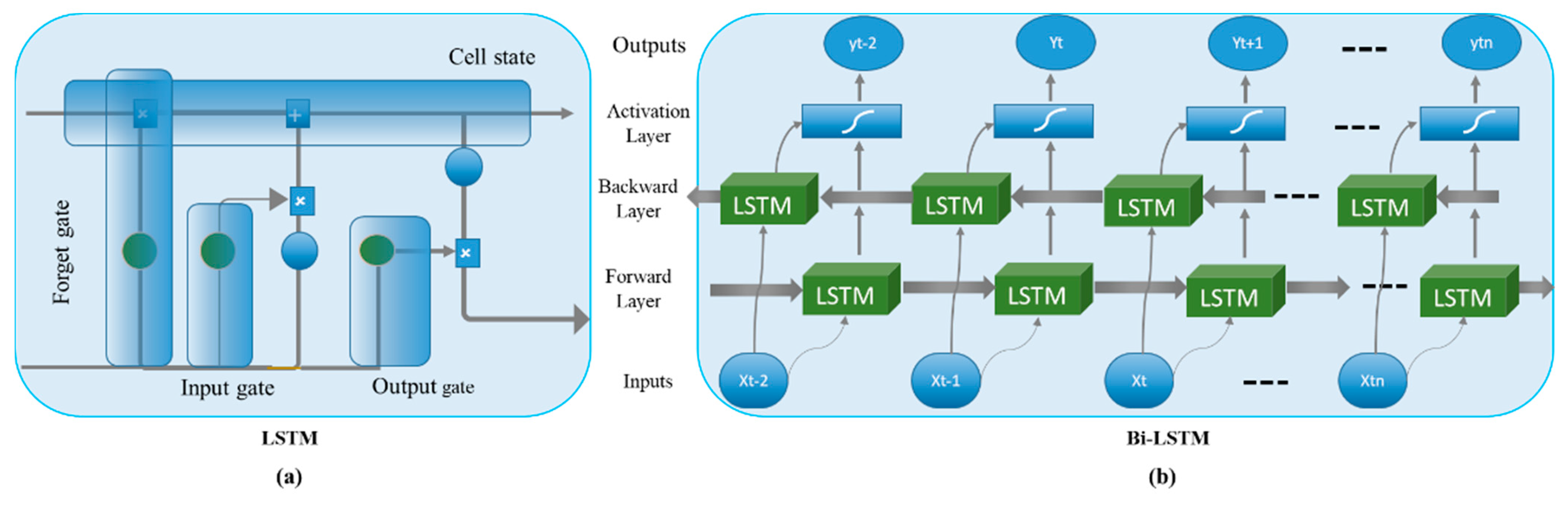
A detailed discussion about the internal architecture of LSTM and its functionality for the information processing is given in this section. LSTM is comprised of special memory blocks in their recurrent layer that overcome the problem of a vanishing gradient. The memory blocks have internal memory cells that are self-connected. These blocks have three multiplicative units known as gates that store the temporal information of the sequence. The three gates are input, output, and forget gate. The input gate controls the flow of current information inside the memory cell, while the output controls the information in the rest of the network. The forget gate sets the state of previous cell information and retains part of the information in the current network. The internal details of the LSTM architecture are given in Figure 3a. The three gates multiply the previous information with a value ranging from 0 to 1. The information is discarded if the value is 0, while retained when the number is 1. The gates use the sigmoid function to turn the data into 0 and 1. This function is given in Equation (5) [40].

$$\sigma \left(x\right)=\frac{1}{1+e^{-x}}$$

(5)

$i_t$, $f_t$, and $o_t$ represent input, forget, and output gate, respectively, while the intermediate value is represented by $C_t$, which can be calculated as follows:

$$i_t=\sigma \left(W_{xi}{x}_t+W_{hi}{h}_{t1}+W_{ci}{C}_{t-1}+b_i\right).$$

(6)

$${\mathrm{i}}_{\mathrm{f}}=\mathsf{\sigma }\left({\mathrm{W}}_{\mathrm{xi}}{\mathrm{x}}_{\mathrm{t}}+{\mathrm{W}}_{\mathrm{hi}}{\mathrm{h}}_{\mathrm{t}1}+{\mathrm{W}}_{\mathrm{ci}}{\mathrm{C}}_{\mathrm{t}-1}+{\mathrm{b}}_{\mathrm{i}}\right)$$

(7)

$${\mathrm{c}}_{\mathrm{t}}={\mathrm{F}}_{\mathrm{XI}}{\mathrm{OC}}_{\mathrm{t}-1}+{\mathrm{I}}_{\mathrm{T}}\mathrm{O}\tan \mathrm{h}({\mathrm{W}}_{\mathrm{XC}}+{\mathrm{W}}_{\mathrm{HC}}{\mathrm{h}}_{\mathrm{t}-1}+{\mathrm{b}}_{\mathrm{C}})$$

(8)

$${\mathrm{o}}_{\mathrm{t}}=\mathsf{\sigma }\left({\mathrm{W}}_{\mathrm{xo}}{\mathrm{x}}_{\mathrm{T}}+{\mathrm{W}}_{\mathrm{ho}}{\mathrm{h}}_{\mathrm{t}-1}+{\mathrm{W}}_{\mathrm{co}}{\mathrm{o}\mathrm{c}}_{\mathrm{t}}+{\mathrm{b}}_{\mathrm{o}}\right)$$

(9)

$${\mathrm{h}}_{\mathrm{t}}={\mathrm{o}}_{\mathrm{t}}\mathrm{o}\tan \mathrm{h}\left({\mathrm{c}}_{\mathrm{t}}\right)$$

(10)

Here, $W_{xi}$, $W_{hi}$, $W_{ci}$, $W_f$, $W_{hf}$, $W_{cf}$, $W_{xo}$, $W_{ho}$, and $W_{co}$ show the weights, while $b_i$, ${\mathrm{b}}_{\mathrm{f}}$, ${\mathrm{b}}_{\mathrm{C}}$, and ${\mathrm{b}}_{\mathrm{o}}$ represent bias vectors. ${\mathrm{x}}_{\mathrm{t}}$ indicates the current input while $\mathrm{t}1$ and ${\mathrm{h}}_{\mathrm{t}-1}$ show the output of information at current time t and previous time $\mathrm{t}-1$, respectively.

Bidirectional LSTM

We also studied and evaluated the performance of bidirectional LSTM for energy consumption, which is another variant of RNNs proposed by Schuster et al. [41]. The core concept of Bi-LSTM can be retrieved from RNNs [41], where the input data sequence is processed in both forward and backward directions inside the hidden layers. Each layer operates using the reversed time-step direction. Basically, two layers operate where one layer processes the sequence in the forward direction while the other layer operates in the backward direction. This representation is given in Figure 3b. This network has widely shown promising results in several fields of ECP and computer vision tasks such as activity analysis [42,43] and forecasting problems. However, M-LSTM is also used for the prediction of energy consumption. In M-LSTM, the state of the first layer obtains the input from the previous layer and the previous state of the same layer. In conventional deep neural networks, the neurons have a huge dimensions in their activation values. These activations have the capability of learning the sequence in big data. Therefore, stacking multiple layers of LSTM guarantees the extraction of long-term sequence information from the data.

4. Results

In this section, we discuss and deeply investigate the experimental results obtained by the proposed method. Similarly, we add the software and implementation details and the data are also structured and analyzed for its usage.

4.1. System Software Settings and Implementation Details

Several kinds of experiments were performed to verify and confirm the effectiveness of the proposed method. The proposed three-tier framework was implemented in Python (Version 3.5) with the famous deep learning framework Keras having TensorFlow as the backend, and Adam was used as an optimizer. We used 10-fold cross-validation during experiments, where the data are divided into N = 10 parts and the N − 1 part is used for testing and the remaining part is used for training. This validation process is repeated until the whole data points are passed from the training and testing phases. Furthermore, we also used the holdout method, where the training and testing sets were formed for validation. Similarly, as we are dealing with a regression problem, we used different error metrics including MSE, RMSE, mean absolute percentage error (MAPE), RMSE, and mean absolute error (MAE). Their detailed formulations are given as follows:

$y_i^{~}$ represents the variable values for n prediction numbers of energy consumption, while $y_i$ shows the observed/predicted values, so Equations (11)–(14) show MSE, MAPE, RMSE, and MAE, respectively.

$$MSE=\frac{1}{n}{\displaystyle \sum }_{i=1}^n{\left(y_i-y_i^{~}\right)}^2$$

(11)

$$MAPE=\frac{100}{n}{\displaystyle \sum }_{i=1}^n|\frac{y_i-y_i^{~}}{y_i}|$$

(12)

$$RMSE=\sqrt{\frac{1}{n}{\displaystyle \sum }_{i=1}^n{\left(y_i-y_i^{~}\right)}^2}$$

(13)

$$MAE=\frac{1}{n}{\displaystyle \sum }_{i=1}^n\left|y_i-y_i^{~}\right|$$

(14)

4.2. Dataset

To evaluate the proposed method, we used the household power consumption dataset.

House Hold Power Consumption Dataset

We used the public power consumption dataset that is available on machine learning UCI repository [44] and consists of data measured through a smart meter in the period of 2006 to 2010, adding up to 4 years of total data. This dataset consists of 2,075,259 instances where 25,979 are missing values, equating to 1.25% of missing data. However, these missing values were handled in the preprocessing step. The data recorded in this dataset are organized in one-minute resolutions over four years. In these data, the total active power is represented using submetering 1, submetering 2, and submetering 3, which are consumed every minute and given in watt-hours. To predict the future energy, we used different resolutions such as minutes, hours, days, and weeks where the input data were given to training network as a series in window sequence. In

Table 5. Detailed description of each attribute in the dataset including units and remarks.

#	Attribute/Unit	Remarks
1	Data/dd.mm.yyyy	This variable represents the date of each instance and includes days, months, and years. The days range from 1 to 30, months from 1 to 12, and years from 2006 to 2010.
2	Time/hh.mm.ss	This variable provides the timing information in minutes, hours, and seconds. The hour resolutions range from 0 to 23 while minute range is from 0 to 59.
3	Global Active Power (GAP)/Kilowatts	The total active power consumed over each appliance in the household in each minute, represented by GAP.
4	Global Reactive Power (GRP)/Kilowatts	The total reactive power consumed over each appliance in the household in each minute, represented by GRP.
5	Voltage(V)/Volts	The total voltage measured in each minute.
6	Global Intensity(GI)/Ampere	The total intensity of current measured in each minute is the GI.
7	Sub-metering(S1)/watt-hours	This energy is related to the power consumed inside the kitchen, which includes the oven, dishwasher, and microwave.
8	Sub-metering(S2)/watt-hours	This energy is related to the power consumed in the laundry room including the refrigerator, washing machine, and tumble-drier.
9	Sub-metering(S3)/watt-hours	The energy consumed to electric water-cooler, heater, and air-conditioner.

, the detailed descriptions of the variables are given and its quantitative details are given in

Table 6. Quantitative structure of the power consumption dataset.

Units	GAB	GRP	V	GI	S1	S2	S3
Mean	1.0916	0.1237	240.83	4.6277	1.1219	1.2985	6.4584
Std	1.0572	0.1127	3.2399	4.4443	6.1530	5.8220	8.4371
Minimum	0.0760	0.0000	223.2000	0.2000	0000	0000	0000
50%	0.6020	0.1000	241.0100	2.6000	0000	000	0000
Maximum	11.1220	0.3900	254.1500	48.4000	88.000	80.000	31.000

.

4.3. Data Interpretation

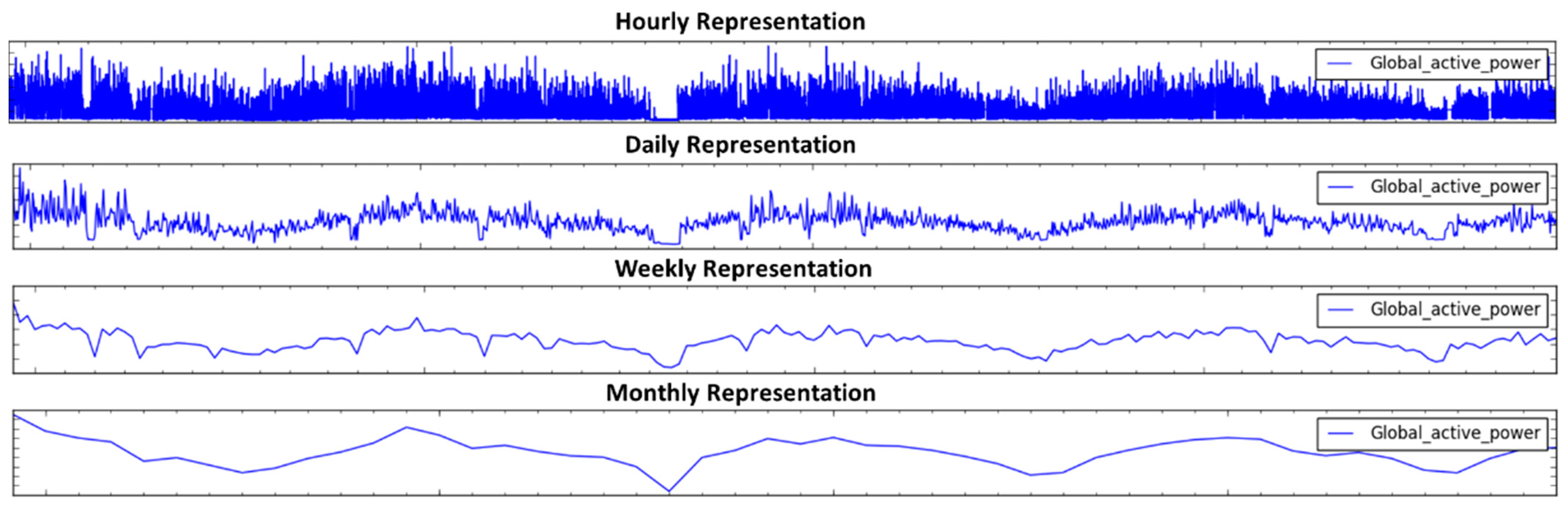
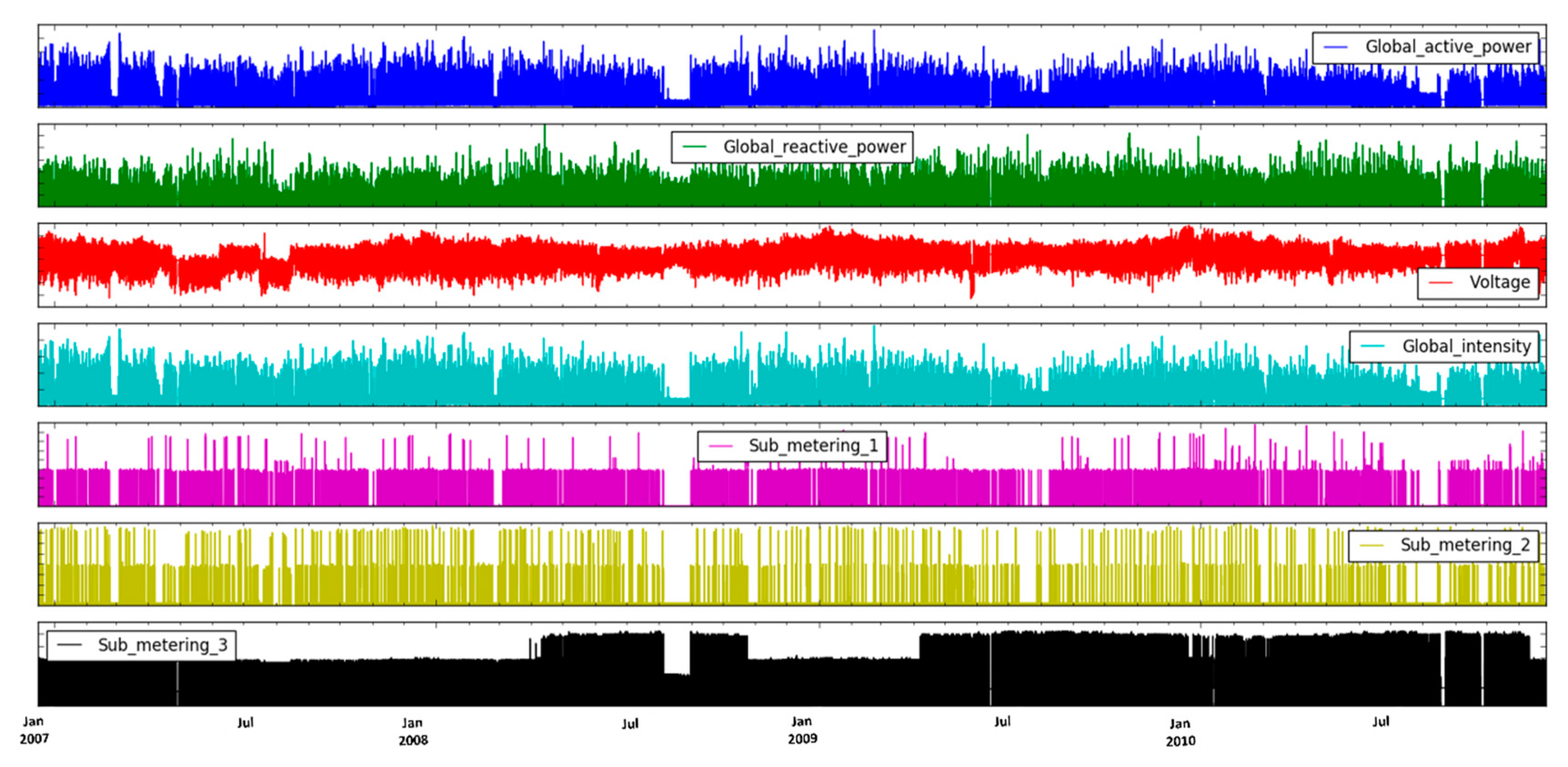
We visualized the variables and analyzed the patterns of each variable as can be seen in Figure 4, which is provided in minute resolutions. This presentation provides a clear interpretation of each variable and the consumption patterns with time. In the proposed method, we totally focused on Global Active Power (GAP), which covers the power consumed over all the appliances; therefore, we further analyzed GAP for its different horizons and its consumption prediction.

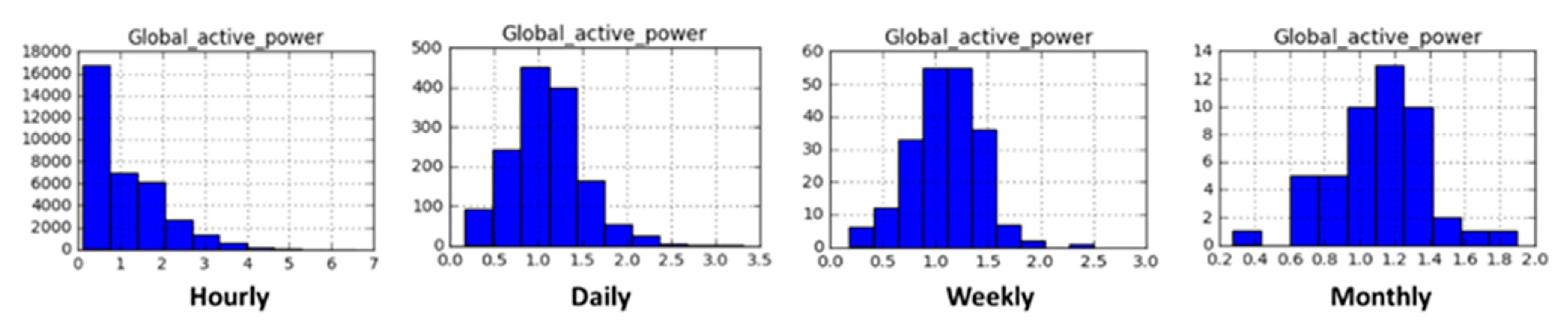
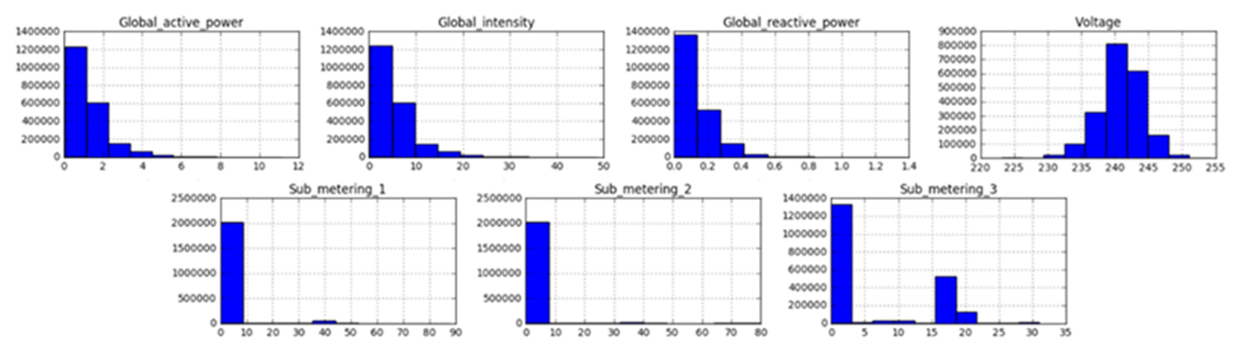
Before feeding the data into the network, it is a significant step to verify and assess the performance of a prediction model to clarify the objectives. Therefore, we created different time horizons of the dataset including hours, days, weeks, and months. For each horizon, an energy prediction was performed. The representation of each horizon is illustrated in Figure 4. In Figure 5, it can be seen that the distribution and observations made in GAP steadily decreased (in kilowatts). Next, Figure 6 represents the visual representation of the data in minutes’ horizons. The distribution is bimodal with a peak, where a long tail is seen in the distribution towards higher values of kilowatts. The drop in energy is observable from Figure 7 when there is no individual at home or all the occupants are asleep, while the peak usage is witnessed when all the appliances in the household are functional. The distribution and the observations made for all variables is given using a histogram in Figure 7.

4.4. Results On ELA

This section discusses the detail experiments carried out using ELAs. We used the K-fold cross-validation method to evaluate the effectiveness of the methods, where the value of K was set 10. In this way, the data were divided into 10 equal parts. K-1 was used for testing and the other K-folds were used for training. At the first, we used the AB algorithm in a practice run to assess its performance against other ELAs. The AB stands for adaptive boosting, which is widely used as an ELA to deal with different regression problems in machine learning. At first, the data were separated into an X- and Y-label to split them. The model was defined as AB regression class and the number of estimators was set as default (n = 50) and the other parameters were set defaults without any change. The metrics used to evaluate its performance are MSE, RMSE, MAE, and MAPE, and the results for the 10-fold method are given in

Table 7. Results obtained using ELA on different horizons using 10-fold method.

Resolution	Method	MSE	RMSE	MAE	MAPE
Minutely	AB	9.6452	3.1056	3.0154	15.3534
	GBR	9.2423	3.0401	2.9235	13.3543
	RF	7.1582	2.6753	2.3433	11.4332
	DT	8.7545	2.9588	2.5454	12.7422
	KNN	8.1876	2.8613	2.7434	12.4212
	SVR	6.0581	2.4613	2.4136	11.2833
Hourly	AB	7.7812	2.7894	2.3443	12.8293
	GBR	7.3241	2.7063	2.2323	10.3721
	RF	5.2962	2.3013	1.9652	11.0038
	DT	6.7941	2.6065	2.5424	9.3432
	KNN	6.1813	2.4862	2.3767	9.4532
	SVR	5.0241	2.2414	2.2385	10.1702
Daily	AB	5.8671	2.4222	2.2561	10.1298
	GBR	5.7631	2.4006	2.30972	8.3421
	RF	4.7652	2.1829	1.9879	9.2313
	DT	5.2321	2.2873	1.9852	8.3431
	KNN	4.9561	2.2262	2.1788	7.7834
	SVR	4.0501	2.0124	1.9413	7.5234
Weekly	AB	4.6532	2.1571	2.0873	7.9363
	GBR	4.3907	2.0953	2.0586	7.7695
	RF	3.7637	1.9400	1.8643	6.9878
	DT	4.3521	2.0861	2.0243	7.1301
	KNN	3.9785	1.9946	1.8732	7.0814
	SVR	3.1321	1.7697	1.6801	6.6231

, while the results of the hold-out method are given in

Table 8. Results obtained using ELA on different horizons using hold-out method.

Resolution	Method	MSE	RMSE	MAE	MAPE
Minutely	AB	8.2145	2.8660	2.1537	14.1932
	GBR	8.0147	2.8310	2.5721	13.7589
	RF	6.2617	2.5023	2.3547	10.5241
	DT	7.3467	2.7104	2.5917	12.1256
	KNN	7.0327	2.6519	2.3147	12.3459
	SVR	5.1394	2.2670	2.0952	10.1568
Hourly	AB	8.5893	2.9307	2.5758	10.4579
	GBR	8.4673	2.9098	2.4849	8.4867
	RF	6.3584	2.5215	2.3217	9.1473
	DT	7.4953	2.7377	2.5874	7.4096
	KNN	7.2934	2.7006	2.3958	7.2851
	SVR	6.1467	2.4792	2.2539	8.0987
Daily	AB	5.3098	2.3043	1.9765	10.0738
	GBR	5.1976	2.2798	1.8764	8.2865
	RF	4.0867	2.0215	1.6938	9.1964
	DT	5.1875	2.2776	1.7456	8.2756
	KNN	4.1583	2.0391	1.1987	7.6483
	SVR	4.0174	2.0043	1.1064	7.4973
Weekly	AB	4.8976	2.2130	1.9897	6.9746
	GBR	4.7756	2.1853	1.9387	6.8645
	RF	3.8275	1.9563	1.7463	5.8674
	DT	4.4984	2.1209	1.9647	6.2365
	KNN	3.9128	1.9780	1.7936	6.1856
	SVR	3.2975	1.8159	1.2975	5.4726

.

The MSE obtained for AB is 9.6452. After AB, we applied GBR to improve the weak learners and create the final prediction model. The DTs were used as base learners in this algorithm. These learners were identified through a gradient in loss function. The prediction made by the weak learner was compared with the actual results to calculate the error. Based on this error, the model defined the gradient and it changed the parameters that decrease the error rate in the next training. Similar to AD, we also used 50 estimators and the same strategy to make X and Y. The MSE value obtained for GBR is 9.2423.

Furthermore, we used RF, which is an ensemble algorithm that is also based on learning of DTs. Here, the estimator fits multiple trees on the extracted subsets and averages their prediction. The number of estimators and the other variables are set to their default values. The RF gives a value of 7.1582 for MSE. Moreover, we evaluated DT, which is a well-known machine learning algorithm most commonly used in regression problems. This model is based on the decision rules that are extracted from the training data. Instead of the class, the model uses and MSE for decision accuracy. DT does not exhibit a good performance in generation and is very sensitive to variation in the training data. A minute change in training data widely affects the prediction accuracy. The minimum number of sample leaves used was 4 and the max depth was set to 2 in the model. The MSE value obtained for DT was 8.7545 in minute resolutions.

KNN is a supervised learning strategy where K is a constant; we used its default value (K = 5). The distance vector of nearest neighbors is computed by its value. The MSE obtained using KNN was 8.1876 in minute resolutions. Similarly, we used SVR which applies a similar procedure as SVM does for regression analysis. As regression data are a continuous number, to fit the model on such data, the SVR approximates the best values with a margin known as epsilon-tube by considering the model complexity and the error rate. The value of MSE in minute resolution in SVR is 6.0581. All these algorithms have different time durations taken during testing and training. These algorithms widely depend on the configuration settings and the data horizons, such as the number of given instances, their resolutions, etc., which affects their timings etc. We calculated the training and testing times of three algorithms such as AB, GBR, and RF. However, the time calculated for AB was used for ABR2 as it the latest version of AB and is used in the proposed method. The time complexity of these algorithms is given in

Table 9. Time complexity analysis of the algorithms.

Algorithm	Training Time (s)	Testing Time (s)
AB	142.8020	0.0140
GBR	591.6442	0.0030
RF	1522.0820	0.0949

, which is calculated for days’ resolutions as we are widely focus on short-term analysis. The analysis carried out for short-term shows that the RF is the most expensive in terms of its training and testing.

4.5. Results On Sequential Learning

In this section, we technically discuss the results obtained for ECP using deep sequential learning and debate on their predictions for future. The same strategy of the K-fold validation method and hold-out method was applied over the used dataset. At first, we performed the experiments on the LSTM network, which is a type of RNN that process the energy sequential data. The LSTM learns the input data sequence by iterating it and acquires the information regarding the observed sequence. Based on learned information, the prediction is performed in the next sequence. We created X and Y sequences in the used dataset and apply the window method with the size of the step value i.e., minutely, hourly, etc. The Y-value was generated after the sequence of X-values. After this, the window was shifted into the next element of X, and then Y was predicted and this process continued.

After applying LSTM, we used Bi-LSTM, which processes the data sequence in forward and backward directions to remember the past information and predict the future data information. We also used M-LSTM where multiple layers of LSTM were used to reduce error and enhance the accuracy and the MSEs obtained for LSTM, Bi-LSTM, and M-LSTM were 0.2821, 0.1855, and 0.1661 in minute resolutions, respectively. These results were obtained using the 10-fold cross-method and are presented in

Table 10. Results obtained for the sequential learning algorithm on different horizons using 10-fold method where the bold values represent the best achieved values.

Resolution	Method	MSE	RMSE	MAE	MAPE
Minutely	LSTM	0.2821	0.5311	0.4941	2.0526
	Bi-LSTM	0.1855	0.4306	0.3214	1.9423
	M-LSTM	0.1661	0.4075	0.3821	1.8666
Hourly	LSTM	0.1986	0.4456	0.4221	1.6435
	Bi-LSTM	0.1329	0.3645	0.3563	1.7575
	M-LSTM	0.1181	0.3436	0.3401	1.4766
Daily	LSTM	0.1502	0.3875	0.3632	1.2323
	Bi-LSTM	0.1423	0.3772	0.3502	1.4731
	M-LSTM	0.1081	0.3287	0.3201	1.4533
Weekly	LSTM	0.1881	0.4337	0.4281	2.4511
	Bi-LSTM	0.1834	0.4282	0.4103	2.1051
	M-LSTM	0.1821	0.4267	0.4201	2.0121

, while the results of the hold-out method are presented in

Table 11. Results obtained for sequential learning algorithm on different horizons using hold-out method.

Resolution	Method	MSE	RMSE	MAE	MAPE
Minutely	LSTM	0.2981	0.5459	0.4756	2.0975
	Bi-LSTM	0.1948	0.4413	0.3963	1.9654
	M-LSTM	0.1479	0.3845	0.3597	1.8794
Hourly	LSTM	0.1784	0.4223	0.4085	1.8275
	Bi-LSTM	0.1285	0.3584	0.3297	1.7367
	M-LSTM	0.1087	0.3296	0.3086	1.4574
Daily	LSTM	0.1684	0.4103	0.3686	1.4586
	Bi-LSTM	0.1583	0.3978	0.3576	1.4368
	M-LSTM	0.1184	0.3440	0.3139	1.3857
Weekly	LSTM	0.1945	0.4410	0.4295	2.4968
	Bi-LSTM	0.1886	0.4342	0.4176	2.1186
	M-LSTM	0.1847	0.4297	0.4132	2.0286

.

4.6. Comparative Analysis

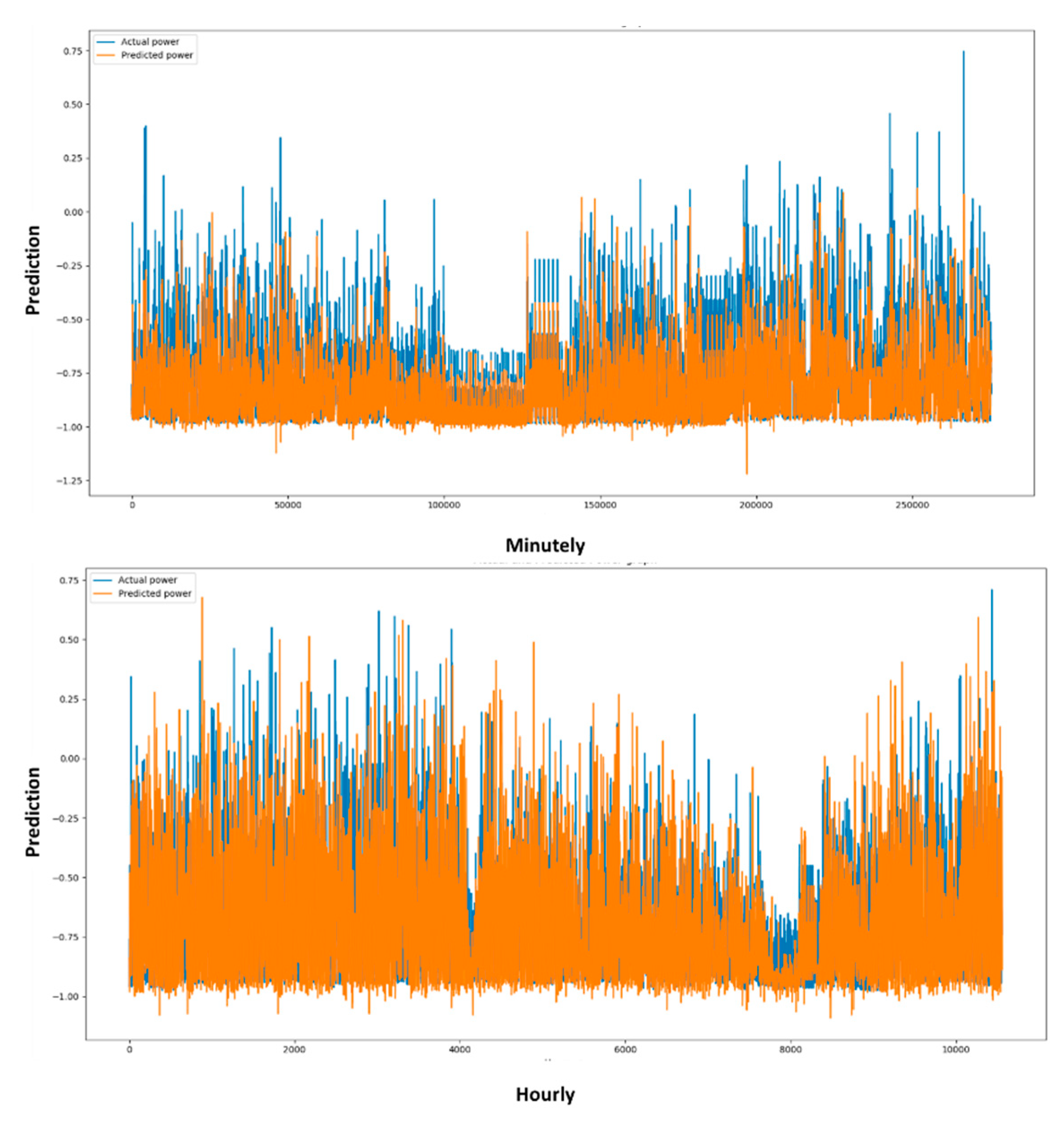
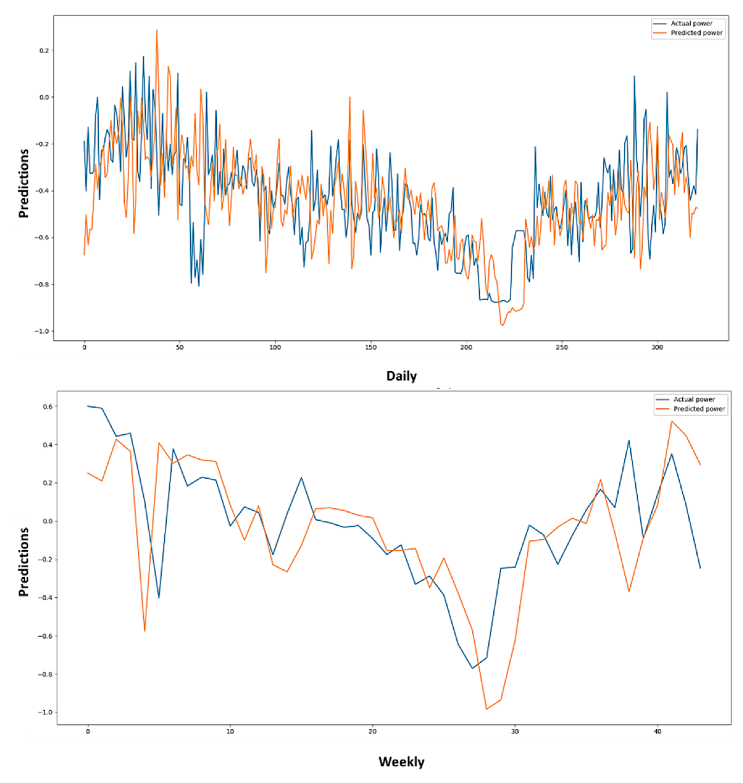
In this section, we compare the techniques used for energy predictions. The employed techniques are generalized as ELA and sequential learning. Sequential learning is known to be a subset of machine learning which functions in a similar fashion. If an algorithm based on artificial intelligence (AI) makes an incorrect prediction, we have to make adjustments. In deep/sequential learning, the algorithms determine on their own whether a prediction is accurate or not using their neural networks. Here, in the prediction problem, the machine learning algorithm parses the data and learns from it to make an informed prediction based on what it has learned. However, the deep sequential learning creates an artificial neural network that learns and makes intelligent predictions. In the proposed study, the sequential learning algorithms perform better than ensemble/conventional machine learning algorithms, which that can be verified by the error values given in Table 7 and Table 10. Additionally, their architectural details are explained in each section, which widely shows the good performance of the deep sequential learning algorithms. The best performers in ensemble learning and sequential learning are SVR and M-LSTM, respectively. Overviewing this, the most appropriate model is M-LSTM from sequential learning. Energy prediction for minutes and hours are given in Figure 8, while for days and week are given in Figure 9. Furthermore, Figure 10 shows a detailed visual representation of the comparative analysis of the methods.

4.7. Comparison with State-of-the-Art Techniques

In this section, we discuss and compare the proposed method with the state of the art to confirm and verify the effectiveness of the proposed algorithm using the household power consumption dataset. To fairly compare the results, we used the same one-minute resolution and the 10-fold results were considered. At first, we investigated the method presented by Kim et al. [45], where a deep learning-based autoencoder was used to forecast future energy by applying backpropagation through a time algorithm and train the model. The MSE and MAE obtained for this method are 0.3840 and 0.3953, respectively. Similarly, a method proposed by Kim et al. [46] formed a hybrid connection of CNNs and LSTM to forecast the residential power and obtained 0.3738 and 0.6114 values for MSE and RMSE, respectively. Similarly, another study by Marino et al. [47] proposed deep neural networks (DNNs) by adding a sequence to sequence architecture LSTM. They used the RMSE metric to evaluate their method and obtained values of 0.5505 and 0.742 for MSE and RMSE, respectively. Furthermore, Mocano et al. [48] investigated stochastic models such as the factored conditional restricted Boltzmann and conditional restricted Boltzmann for the energy forecasting problem and obtained values of 0.4439 and 0.666 for MSE and RMSE. Finally, we pose our proposed results where the obtained MSE, RMSE, MAE, and MAPE values are 0.1661, 0.4075, 0.3821, and 1.8666, respectively. The overall comparison is shown in

Table 12. Comparative analysis of the proposed method with state-of-the-art methods where the bold wording represents the proposed results.

Ref	Evaluation Metrics
	MSE	RMSE	MAE	MAPE
[45]	0.3840	0.6196	0.395	---
[46]	0.3738	0.611	0.349	0.3484
[47]	0.5505	0.742	----	----
[48]	0.4439	0.6663	----	----
Proposed method	0.1661	0.4075	0.3821	1.8666

.

5. Conclusions

The technological growth and industrial electrical machineries advancements have resulted in a large amount of energy consumption in terms of power, fuel, oil, and gas without proper infrastructure. The practice of smart energy management over the decades has received considerably lower research attention when compared to computer vision and many other data science problems. A large amount of energy is wasted due to improper management and no proper adjustment being made between the residential buildings/areas and smart grids. To handle this problem, researchers apply several techniques to forecast and efficiently manage energy consumption through machine learning techniques. Though, the existing techniques have widely focused on the study of a single strategy and are selective for conventional approaches, their performance is still far from real-world implementation. Thus, in this paper, we developed a three-tier novel ECP framework and we dive deep into a detailed comparative analysis of conventional and deep sequential forecasting learning methods by investigating them for predictions and error rates. Conventional forecasting learning includes several ELAs while deep sequential learning contains popular techniques such as LSTM, Bi-LSTM, and M-LSTM. In the first tier, the input data sequence is given to preprocessing layer for noise and outlier removal. The second tier feds the refined data into the training phase for learning while the third tier gives the final ECP through actual and prediction graphs. We also evaluated the effectiveness of the proposed method using basic error metrics. Furthermore, we visualized the data and the results to analyze the data patterns that show better interpretations. The proposed method used individual a household power consumption dataset that is publicly available on UCI machine learning repository.

In future, we aim to consider different forms of energy acquired from the real-world environment such as temperature, humidity, heating, cooling, energy from solar, water, and wind related data. Based on these data, we aim to explore distinct forecasting models using mathematical and theoretical modeling, AI, complex neural networks, and reinforcement learning. Similarly, energy storage systems are important aspects to be considered in energy management to aid efficient energy consumption. Next, the energy generation is not properly aligned with the residential areas for proper energy usage; therefore, a system to match the smart grid and residential areas for energy production and consumption need to be included in the energy related literature. Moreover, we intend to focus on edge computing and include resource-constrained devices with lower computational costs. Using the edge concept will ease ECPs in terms of lower compositionality and ensure timely responses.

References

- Amasyali, K.; El-Gohary, N.M. A review of data-driven building energy consumption prediction studies. Renew. Sustain. Energy Rev. 2018, 81, 1192–1205. [Google Scholar] [CrossRef]
- Bhuniya, S.; Sarkar, B.; Pareek, S. Multi-product production system with the reduced failure rate and the optimum energy consumption under variable demand. Mathematics 2019, 7, 465. [Google Scholar] [CrossRef] [Green Version]
- Fumo, N.; Mago, P.; Luck, R. Methodology to estimate building energy consumption using EnergyPlus Benchmark Models. Energy Build. 2010, 42, 2331–2337. [Google Scholar] [CrossRef]
- Yodwong, B.; Thounthong, P.; Guilbert, D.; Bizon, N. Differential flatness-based cascade energy/current control of battery/supercapacitor hybrid source for modern e–vehicle applications. Mathematics 2020, 8, 704. [Google Scholar] [CrossRef]
- Zhang, L.; Li, Y.; Stephenson, R.; Ashuri, B. Valuation of energy efficient certificates in buildings. Energy Build. 2018, 158, 1226–1240. [Google Scholar] [CrossRef]
- Pan, Y.; Zhang, L.; Wu, X.; Zhang, K.; Skibniewski, M.J. Structural health monitoring and assessment using wavelet packet energy spectrum. Saf. Sci. 2019, 120, 652–665. [Google Scholar] [CrossRef]
- Kim, S.; Kim, S. A multi-criteria approach toward discovering killer IoT application in Korea. Technol. Forecast. Soc. Chang. 2016, 102, 143–155. [Google Scholar] [CrossRef]
- Malik, S.; Kim, D. Prediction-learning algorithm for efficient energy consumption in smart buildings based on particle regeneration and velocity boost in particle swarm optimization neural networks. Energies 2018, 11, 1289. [Google Scholar] [CrossRef] [Green Version]
- Zhong, H.; Wang, J.; Jia, H.; Mu, Y.; Lv, S. Vector field-based support vector regression for building energy consumption prediction. Appl. Energy 2019, 242, 403–414. [Google Scholar] [CrossRef]
- Guo, Y.; Wang, J.; Chen, H.; Li, G.; Liu, J.; Xu, C.; Huang, R.; Huang, Y. Machine learning-based thermal response time ahead energy demand prediction for building heating systems. Appl. energy 2018, 221, 16–27. [Google Scholar] [CrossRef]
- Liu, Z.; Wu, D.; Liu, Y.; Han, Z.; Lun, L.; Gao, J.; Jin, G.; Cao, G. Accuracy analyses and model comparison of machine learning adopted in building energy consumption prediction. Energy Explor. Exploit. 2019, 37, 1426–1451. [Google Scholar] [CrossRef] [Green Version]
- Zhang, Y.; Zhang, X.; Tang, L. Energy Consumption Prediction in Ironmaking Process Using Hybrid Algorithm of SVM and PSO. In Proceedings of the International Symposium on Neural Networks, Shenyang, China, 11–14 July 2012; pp. 594–600. [Google Scholar]
- De Cauwer, C.; Van Mierlo, J.; Coosemans, T. Energy consumption prediction for electric vehicles based on real-world data. Energies 2015, 8, 8573–8593. [Google Scholar] [CrossRef]
- Cai, H.; Shen, S.; Lin, Q.; Li, X.; Xiao, H. Predicting the energy consumption of residential buildings for regional electricity supply-side and demand-side management. IEEE Access 2019, 7, 30386–30397. [Google Scholar] [CrossRef]
- Fumo, N.; Biswas, M.R. Regression analysis for prediction of residential energy consumption. Renew. Sustain. Energy Rev. 2015, 47, 332–343. [Google Scholar] [CrossRef]
- Luo, J.; Hong, T.; Fang, S.-C. Benchmarking robustness of load forecasting models under data integrity attacks. Int. J. Forecast. 2018, 34, 89–104. [Google Scholar] [CrossRef]
- Zhang, Y.; Lin, F.; Wang, K. Robustness of Short-Term Wind Power Forecasting Against False Data Injection Attacks. Energies 2020, 13, 3780. [Google Scholar] [CrossRef]
- Khan, N.; Ullah, F.U.M.; Ullah, A.; Lee, M.Y.; Baik, S.W. Batteries State of Health Estimation via Efficient Neural Networks with Multiple Channel Charging Profiles. IEEE Access 2020, 9, 7797–7813. [Google Scholar] [CrossRef]
- He, Y.; Wu, P.; Li, Y.; Wang, Y.; Tao, F.; Wang, Y. A generic energy prediction model of machine tools using deep learning algorithms. Appl. Energy 2020, 275, 115402. [Google Scholar] [CrossRef]
- Hu, H.; Wang, L.; Lv, S.-X. Forecasting energy consumption and wind power generation using deep echo state network. Renew. Energy 2020, 154, 598–613. [Google Scholar] [CrossRef]
- Ullah, A.; Haydarov, K.; Haq, I.U.; Muhammad, K.; Rho, S.; Lee, M.; Baik, S.W. Deep Learning Assisted Buildings Energy Consumption Profiling Using Smart Meter Data. Sensors 2020, 20, 873. [Google Scholar] [CrossRef] [Green Version]
- Gao, Y.; Ruan, Y.; Fang, C.; Yin, S. Deep learning and transfer learning models of energy consumption forecasting for a building with poor information data. Energy Build. 2020, 223, 110156. [Google Scholar] [CrossRef]
- Somu, N.; MR, G.R.; Ramamritham, K. A hybrid model for building energy consumption forecasting using long short term memory networks. Appl. Energy 2020, 261, 114131. [Google Scholar] [CrossRef]
- Hussain, T.; Min Ullah, F.U.; Muhammad, K.; Rho, S.; Ullah, A.; Hwang, E.; Moon, J.; Baik, S.W. Smart and intelligent energy monitoring systems: A comprehensive literature survey and future research guidelines. Int. J. Energy Res. 2021, 45, 3590–3614. [Google Scholar] [CrossRef]
- Li, K.; Xie, X.; Xue, W.; Dai, X.; Chen, X.; Yang, X. A hybrid teaching-learning artificial neural network for building electrical energy consumption prediction. Energy Build. 2018, 174, 323–334. [Google Scholar] [CrossRef]
- Ullah, F.U.M.; Ullah, A.; Haq, I.U.; Rho, S.; Baik, S.W. Short-term prediction of residential power energy consumption via CNN and multi-layer bi-directional LSTM networks. IEEE Access 2019, 8, 123369–123380. [Google Scholar] [CrossRef]
- Wen, L.; Zhou, K.; Yang, S.; Lu, X. Optimal load dispatch of community microgrid with deep learning based solar power and load forecasting. Energy 2019, 171, 1053–1065. [Google Scholar] [CrossRef]
- Tidemann, A.; Høverstad, B.A.; Langseth, H.; Öztürk, P. Effects of Scale on Load Prediction Algorithms. In Proceedings of the 22nd International Conference and Exhibition on Electricity Distribution, Stockholm, Sweden, 10–13 June 2013. [Google Scholar]
- Haben, S.; Ward, J.; Greetham, D.V.; Singleton, C.; Grindrod, P. A new error measure for forecasts of household-level, high resolution electrical energy consumption. Int. J. Forecast. 2014, 30, 246–256. [Google Scholar] [CrossRef] [Green Version]
- Freund, Y.; Schapire, R.E. A decision-theoretic generalization of on-line learning and an application to boosting. J. Comput. Syst. Sci. 1997, 55, 119–139. [Google Scholar] [CrossRef] [Green Version]
- Drucker, H. Improving regressors using boosting techniques. ICML 1997, 97, 107–115. [Google Scholar]
- Freund, Y.; Schapire, R.; Abe, N. A short introduction to boosting. J.-Jpn. Soc. Artif. Intell. 1999, 14, 1612. [Google Scholar]
- Mac Namee, B.; Cunningham, P.; Byrne, S.; Corrigan, O.I. The problem of bias in training data in regression problems in medical decision support. Artif. Intell. Med. 2002, 24, 51–70. [Google Scholar] [CrossRef]
- Friedman, J.H. Greedy function approximation: A gradient boosting machine. Ann. Stat. 2001, 29, 1189–1232. [Google Scholar] [CrossRef]
- Natekin, A.; Knoll, A. Gradient boosting machines, a tutorial. Front. Neurorobot. 2013, 7, 21. [Google Scholar] [CrossRef] [Green Version]
- Ho, T.K. Random Decision Forests. In Proceedings of the 3rd International Conference on Document Analysis and Recognition, Montreal, QC, Canada, 14–16 August 1995; pp. 278–282. [Google Scholar]
- Breiman, L. Random forests. Mach. Learn. 2001, 45, 5–32. [Google Scholar] [CrossRef] [Green Version]
- Soucy, P.; Mineau, G.W. A simple KNN algorithm for text categorization. In Proceedings of the 2001 IEEE International Conference on Data Mining, San Jose, CA, USA, 29 November–2 December 2001; pp. 647–648. [Google Scholar]
- Quinlan, J.R. Induction of decision trees. Mach. Learn. 1986, 1, 81–106. [Google Scholar] [CrossRef] [Green Version]
- Graves, A. Long Short-Term Memory. In Supervised Sequence Labelling with Recurrent Neural Networks; Springer: Berlin, Geermany, 2012; pp. 37–45. [Google Scholar]
- Schuster, M.; Paliwal, K.K. Bidirectional recurrent neural networks. IEEE Trans. Signal Process. 1997, 45, 2673–2681. [Google Scholar] [CrossRef] [Green Version]
- Ullah, F.U.M.; Ullah, A.; Muhammad, K.; Haq, I.U.; Baik, S.W. Violence detection using spatiotemporal features with 3D convolutional neural network. Sensors 2019, 19, 2472. [Google Scholar] [CrossRef] [Green Version]
- Sajjad, M.; Nasir, M.; Ullah, F.U.M.; Muhammad, K.; Sangaiah, A.K.; Baik, S.W. Raspberry Pi assisted facial expression recognition framework for smart security in law-enforcement services. Inf. Sci. 2019, 479, 416–431. [Google Scholar] [CrossRef]
- Georges Hebrail, A.B. Individual Household Electric Power Consumption Data Set. 2012. Available online: https://archive.ics.uci.edu/ml/datasets/individual+household+electric+power+consumption (accessed on 29 December 2020).
- Kim, J.-Y.; Cho, S.-B. Electric energy consumption prediction by deep learning with state explainable autoencoder. Energies 2019, 12, 739. [Google Scholar] [CrossRef] [Green Version]
- Kim, T.-Y.; Cho, S.-B. Predicting residential energy consumption using CNN-LSTM neural networks. Energy 2019, 182, 72–81. [Google Scholar] [CrossRef]
- Marino, D.L.; Amarasinghe, K.; Manic, M. Building energy load forecasting using deep neural networks. In Proceedings of the IECON 2016-42nd Annual Conference of the IEEE Industrial Electronics Society, Florence, Italy, 23–26 October 2016; pp. 7046–7051. [Google Scholar]
- Mocanu, E.; Nguyen, P.H.; Gibescu, M.; Kling, W.L. Deep learning for estimating building energy consumption. Sustain. Energy Grids Netw. 2016, 6, 91–99. [Google Scholar] [CrossRef]
Figure 1.
Overview of a smart grid operation and the statistical details energy consumption in different sectors. (a) Renewable energy is obtained by the smart grid, where it is organized and made suitable for usage. After passing the data from the initial stages, it is supplied to the consumers according to their demands. These consumers include industries, households, offices, and public transport systems. (b) The statistical overview of the energy used in different sectors of South Korea, where the industries consume huge amount of energy due to heavy machinery.
Figure 2.
Three-tier ECP framework. At first, the preprocessing step is applied for noise and outlier removal from the data, normalization, and formation of horizons. In the second tier, the model’s learning is carried, which comprises of conventional learning and sequential learning-based methods, while the third tier gives the final prediction of energy, visualization, and performance evaluation using basic metrics.
Figure 3.
Internal architecture of sequential learning methods. (a) The internal architecture of the LSTM and the data flow using the internal gates. (b) Bi-LSTM with input, internal layers, and output layers showing forward and backward passes.
Figure 4.
Visual presentation of total active power in the household dataset.
Figure 5.
Detailed analysis using histogram where the Global Active Power (GAP) distribution is skewed towards low values.
Figure 6.
Visual representation of each variable used in household power consumption dataset in minute resolutions. We found that there are missing values present in the years 2007, 2009, and 2010. A decreasing trend was observed each year from July to August, while an increasing trend was seen in the month of September.
Figure 7.
Histogram obtained for each variable in the dataset, given in minutes’ resolutions.
Figure 8.
Graphical representation of the prediction of energy based on actual data used. The prediction was obtained using proposed method M-LSTM on different resolutions such as minutes and hours.
Figure 9.
Graphical representation of the prediction of energy based on actual data used. The prediction was obtained using the proposed method M-LSTM on different resolutions such as minutes and hours.
Figure 10.
Visual representation of each method using MSE and RMSE for the minutes’ horizon, which shows the better performance of the deep sequential learning algorithms over ELA.