Sequential Learning-Based Energy Consumption Prediction Model for Residential and Commercial Sectors

Abstract

The use of electrical energy is directly proportional to the increase in global population, both concerning growing industrialization and rising residential demand. The need to achieve a balance between electrical energy production and consumption inspires researchers to develop forecasting models for optimal and economical energy use. Mostly, the residential and industrial sectors use metering sensors that only measure the consumed energy but are unable to manage electricity. In this paper, we present a comparative analysis of a variety of deep features with several sequential learning models to select the optimized hybrid architecture for energy consumption prediction. The best results are achieved using convolutional long short-term memory (ConvLSTM) integrated with bidirectional long short-term memory (BiLSTM). The ConvLSTM initially extracts features from the input data to produce encoded sequences that are decoded by BiLSTM and then proceeds with a final dense layer for energy consumption prediction. The overall framework consists of preprocessing raw data, extracting features, training the sequential model, and then evaluating it. The proposed energy consumption prediction model outperforms existing models over publicly available datasets, including Household and Korean commercial building datasets.

1. Introduction

The precise prediction of energy consumption in residential and industrial sectors assists smart homes and grids to manage the demand of occupants efficiently and establish policies for energy preservation. Therefore, energy load forecasting for smart grids has become a hot research area and a top priority for smart city development [1]. Smart grids are responsible for the distribution of power acquired from different sources at different levels depending on consumption and future demand [2]. The overall chain of electrical energy consists of three stages—production at power plants, management/distribution at grids, and consumption in various sectors [3]. Hence, the smart grid is the main hub acting as a supervisor to keep the balance or act as a bridge between production and consumption through using appropriate scheduling and management policies to avoid wasteful energy generation and financial loss [4]. For this purpose, energy forecasting methods play a key role in maintaining stability and ensuring proper planning between producers and consumers [5]. Similarly, the costs of unpredictability and noisy data acquired from metering devices sometimes result in wrong predictions, which cause severe economic damage. For instance, UK power authorities reported a 10-million-pound loss per year in 1984 due to a 1% increase in forecasting error [6]. Therefore, numerous prediction models have been proposed that are mainly focused on reducing the prediction error rate and improving the quality of the power grids by optimizing energy use.

Sustainable buildings and construction are making progress in terms of energy preservation, but developments remain out of step with the growth of the construction sector and the rising demand for energy services [7]. Therefore, urban planners must adopt ambitious energy planning policies to ensure that future construction is carried out in a way that increases energy efficiency in buildings [8]. In this regard, energy consumption prediction and demand response management play an important role in analyzing each influencing factor that leads to energy preservation and reduces its impact on the environment [9]. Moreover, energy consumption prediction models can help in understanding the impact of energy retrofitting and energy supply programs because these models can be used to define energy requirements as a function of input parameters [10]. These factors make the energy predictive models the most useful tool for energy managers, urban planners, and policymakers when establishing national or regional energy supply requirements. On a smaller scale, they can be used to determine changes in energy demand for specific buildings. Hence, policy decisions related to building-sector energy can be enhanced using these forecasting models in sustainable urban or smart city development projects [11].

Power consumption forecasting is a multivariate time series data analysis task that is affected by various factors such as weather and occupant behavior. These make it difficult for machine learning techniques to learn the data pattern sequences for energy forecasting [12]. On the other hand, deep learning models have shown tremendous results in many complex domains such as image/video [13], audio [14], and text [15] processing applications and with prediction and estimation problems [16]. During the last few years, researchers from these domains have developed hybrid deep models by integrating the features of multiple deep models or combing the architectures to achieve higher accuracy. Similarly, a number of different hybrid deep models have been developed for energy consumption prediction [17,18]. However, there is still room for accuracy enhancement with minimum resource utilization. Therefore, in this study, we conducted a comparative analysis of sequential learning models to select the optimum proposed model. The key contributions of this study are summarized as follows:

• A comparative study is conducted over sequential learning models to select the optimum combination with deep features for energy consumption prediction;
• The input dataset is passed through a preprocessing phase in which redundant data are removed and the missing values are filled with corresponding data values from the previous 24 h. Next, the data are normalized to achieve adequate predictive results;
• A novel hybrid architecture combining ConvLSTM with BiLSTM is proposed in which ConvLSTM extracts and encodes spatial characteristics from input data and BiLSTM decodes these characteristics for forecasting;
• The experimental results show that the proposed architecture has the best performance in comparison to other models. The measurement metrics report the lowest energy-consumption prediction value for mean squared error (MSE), mean absolute error (MAE), root mean square error (RMSE), and mean absolute percentage error (MAPE).

The rest of the paper is organized as follows. Section 2 represents the related research for technical forecasting of energy consumption. Section 3 represents the technical details of the proposed framework, followed by experimental results in Section 4. Finally, the paper is concluded in Section 5 along with some future research directions.

2. Literature Review

Employed energy forecasting methods can be categorized into two classes—statistical and deep learning-based. Recently, comprehensive surveys on energy forecasting have been published by Fallah et al. [19], covering methods from 2001 to 2019, and Hussain et al. [20], covering the related methods from 2011 to 2020. However, in this paper, we explored only deep learning-based literature due to their tremendous contributions in forecasting models, especially for time series data. For instance, Kong et al. [21] analyzed resident behavior learning with long short-term memory (LSTM) to propose a short-term load forecasting (STLF) model. The basic theme of this paper was to overcome the challenging problem of variant behavior of the residential loads that hinder the precise prediction results. Similarly, Almalaq and Zhang [22] proposed a hybrid technique by integrated deep learning and genetic algorithm with LSTM for energy forecasting of residential buildings. Kim and Cho [23] presented a hybrid energy prediction model in which two layers of convolutional neural network (CNN) are used to extract the complex features and then a simple LSTM [24] for sequence learning is adopted followed by a dense layer for final prediction. This study is further improved by Khan et al. [17], who used an LSTM autoencoder (LSTM-AE) instead of a simple LSTM and reported that their model is more efficient in terms of time complexity.

Another hybrid model is presented by Le et al. [25] in which deep features from CNN were forwarded to BiLSTM in both forward and backward directions. This study is further extended by Ullah et al. [26], who used a multi-layer BiLSTM for sequential learning. Wen et al. [27] integrated a deep recurrent neural network with LSTM for the forecasting of power load at solar-based microgrids. A swarm algorithm was then applied to the sequential data from LSTM for an optimized load dispatched by the connected grids. Kim and Cho [18] extracted features for energy consumption data using CNN and then forwarded these features to state expendable autoencoder for future consumption predictions based on 15-, 30-, 45-, and 60-min resolutions. Recently, Sajjad et al. [28] proposed a hybrid sequential learning model for energy forecasting by integrating CNN and gated recurrent units (GRU) into a unified framework for accurate energy consumption prediction.

Energy forecasting has an important role in the formulation of successful policies to efficiently use natural resources. For instance, Rahman et al. [29] presented an approach for the prediction of the total energy consumption in India to assist the policymakers for energy management. Their proposed model is based on the simple regression model (SRM) and multiple linear regression (MLR) along with other techniques that give satisfying results. Similarly, Jain et al. [30] proposed a support vector regression (SVR) based machine learning approach for the energy prediction of the multi-family residential buildings in one of the dense city New York. Zheng et al. [31] presented a hybrid LSTM-based model along with the selection of similar days and empirical mode decomposition (EMD) for the short-term load prediction of the electricity. Chujai et al. [32] proposed autoregressive integrated moving average (ARIMA) and autoregressive moving average (ARMA) models for power consumption forecasting. The ARIMA model demonstrated efficient results for monthly power consumption forecasting, while the ARMA model has the advantages of daily and weekly forecasting. Kim et al. [23] combined CNN with LSTM and presented a hybrid CNN–LSTM neural network approach for energy prediction with a very small RMSE value.

In real-time energy forecasting, a proper plan is needed to accomplish the demand of consumers and operate electrical appliances without any problems. For this management, Muralitharan et al. [33] proposed a model for the prediction of consumer demand based on CNN and genetic algorithm techniques, which reveal convincing results for short-term forecasting. Similarly, Aslam et al. [34] developed a trust-worthy energy management system by utilizing mixed-integer linear programming (MILP) and also established a friendly environment between consumers and energy generation. Bourhnane et al. [35] presented a model for energy forecasting and scheduling in smart buildings by integrating artificial neural network (ANN) and genetic algorithms. Further, they also tested the model in real-time, which produced incredible output for both short- and long-term forecasting. This study is further improved by Somu et al. [36], proposing a novel forecasting model by employing LSTM with a robust sine cosine algorithm for the prediction of heterogeneous data in an efficient way. Sometimes, smart sensor devices generated unusual data due to numerous weather conditions; therefore, Shao et al. [37] fine-tuned the support vector machine (SVM) by handling two extra parameters, including weather and air-conditioning system, to prove the model stability on critical input values. Another precise energy consumption prediction in real-time was achieved in a study by Ruiz et al. [38] in which clustering techniques were applied to select the optimal one for analyzing discriminative patterns from data. In addition, to extract temporal features from raw input data, Fang et al. [39] followed a hybrid approach by incorporating LSTM and domain adversarial neural network (DANN) that mainly focuses on relevant features. They verified the performance of transfer learning strategy and domain adaptability through various experiments. Short- and long-term energy forecasting strategies have a significant role in the energy sector because they meet the energy required on the consumer side. Therefore, Hu et al. [40] introduced a novel deep learning idea by combining non-linear and stacked hierarchy models to analyze and authenticate the model reliability. Summarizing the con and pros of the energy forecasting models in the literature, we conclude that in contrast to traditional machine learning approaches, the above-mentioned deep sequential learning models for energy show good performance in terms of reduced error rates. However, there still exist several sequential models that have not yet been explored. Hence, an optimum hybrid model is still in need to achieve better accuracy with a small amount of resource utilization.

3. Proposed Framework

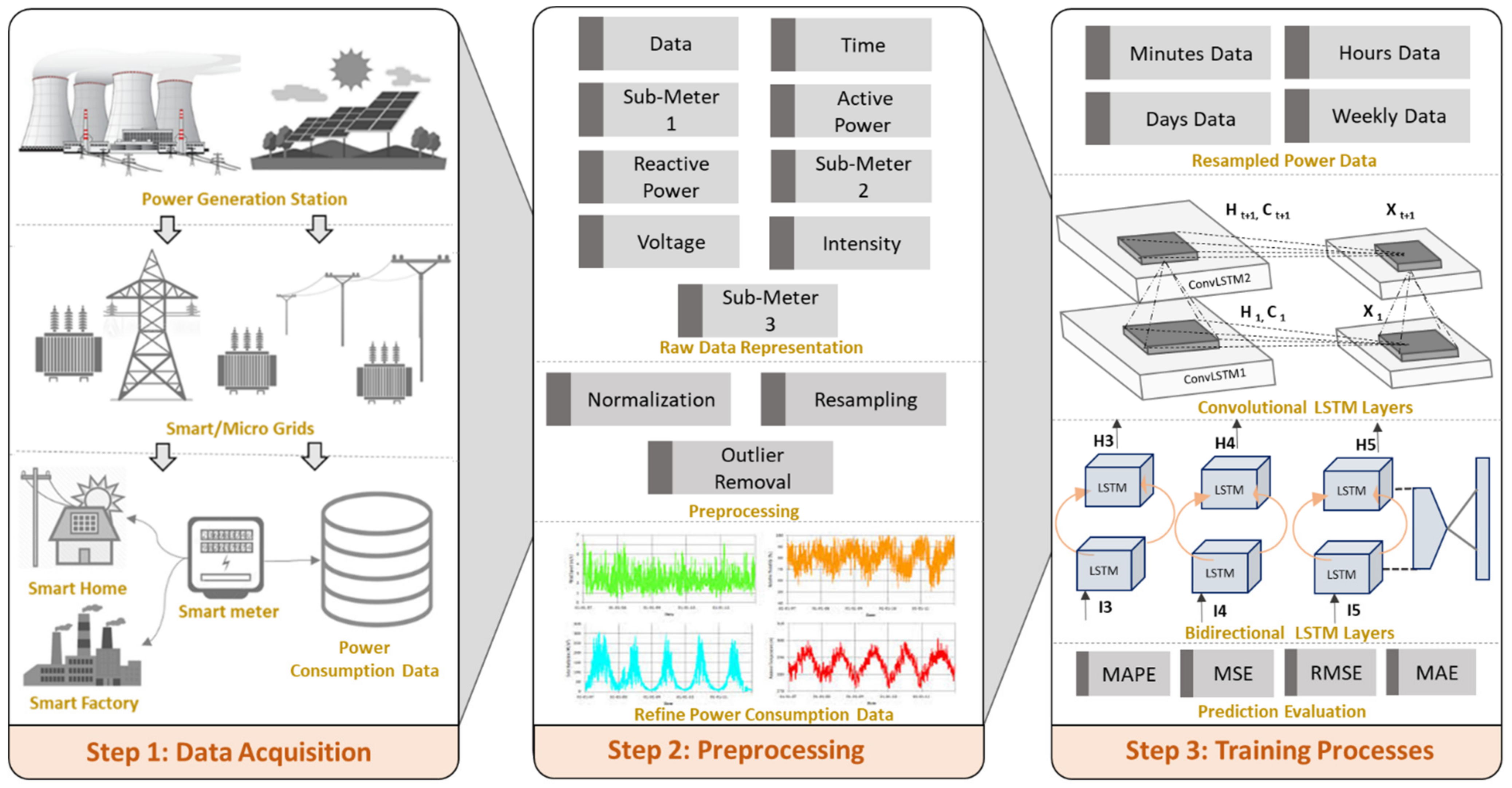
Precise forecasting of energy consumption in commercial and residential buildings assists smart grids to efficiently manage the demand of occupants and conserve energy for the future. Several traditional sequential learning forecasting models have been developed for energy consumption forecasting that reveal inadequate performance due to the utilization of unclean data. These approaches face various problems while learning parameters from scratch, such as overfitting, and short-term memory difficulties, such as data increases or the association between variables, become more complex [41]. These problems can be easily tackled through sequential learning models that have the ability to capture spatial and temporal patterns from smart meters data at once. Based on this assumption, we developed a novel forecasting framework that provides a useful way to overcome the energy forecasting problem. The overall dataflow of the proposed framework is divided into three steps, as shown in Figure 1. First, the total consumed energy data are obtained from smart meters/sensors that contain abnormalities due to external influence. Next, data cleansing techniques are applied to the collected data in preprocessing step for eliminating the abnormalities. In the final step, the preprocessed data are fed into the one-dimensional ConvLSTM for features encoding, followed by the BiLSTM network that efficiently decodes the feature maps and learns the sequence patterns. The proposed framework is evaluated on various resolutions of data, i.e., minutely, hourly, daily, and weekly for short- and long-term forecasting using common error evaluation metrics. A detailed description of each step of the proposed framework is provided in the following subsections.

3.1. Data Acquisition and Preprocessing

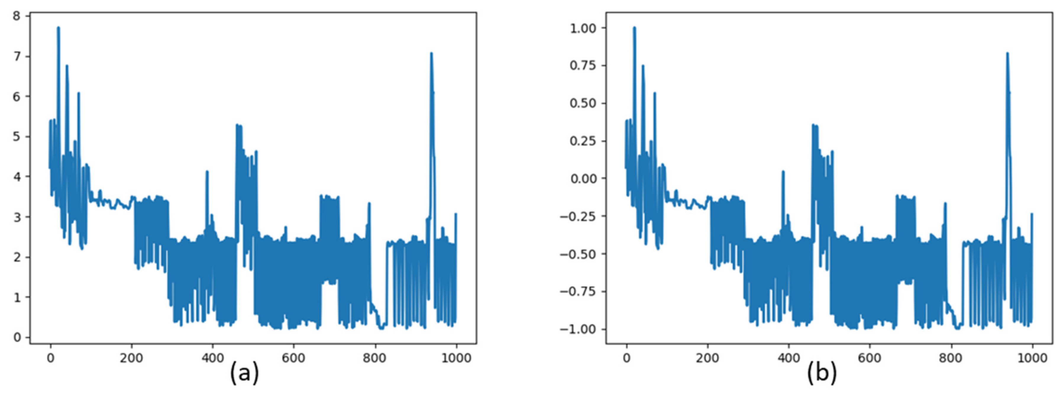
This section provides a detailed description of the data collection and preprocessing strategy. Recent studies have shown that the performance of trained artificial intelligence (AI) models depend on the input data. Therefore, if the smart meter’s data are well polished and organized, they can assist in training any model of AI in a more convenient way. The consumed energy data obtained from meters installed on each floor of a residential building is stored in a raw, incomplete, and non-organized format. Moreover, sometimes the data contain abnormalities due to wire break, occupant’s behavior, and weather condition. Hence, using these data directly for energy consumption forecasting degrades the overall performance of the model. Therefore, we first passed the obtained data to the preprocessing step in which missing values are handled by replacing subsequent values. The pre- and post-processing data distributions are shown in Figure 2; we removed noise from the data and normalize them via min–max process while the outliers are detected and removed using the standard deviation method. There are 1.25% missing values in the Household Dataset, which are filled with the corresponding values of the previous 24-h data.

3.2. ConvLSTM for Data Encoding

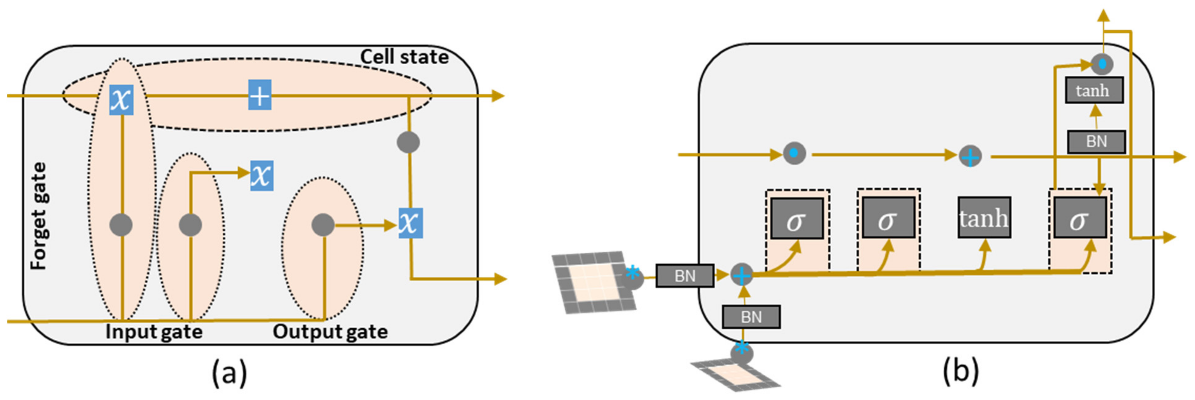
Fully connected LSTM is one of the effective approaches to manage the sequential correlations in data; however, it contains massive redundancy for spatial data, which is not able to handle spatiotemporal information [42]. To tackle such a problem, we utilized the extended version of fully connected LSTM called ConvLSTM [43], which has a convolutional structure in input and state-to-state transition having the ability to preserve the spatial characteristics of the data. In this study, we arranged multiple ConvLSTM layers to build generalize encoding model that can be utilized for forecasting problems and for spatiotemporal, sequence-to-sequence prediction. For instance, fully connected LSTM handles the spatiotemporal data by converting it into a 1D vector that results in a vital loss in sequence information. In contrast, ConvLSTM takes input in a 3D format in which it keeps spatial sequential data in the last dimension. In addition, the next state of a specific cell is dependent on previous and input states that can be obtained by convolutional operators for both state-to-state and input-to-state transitions. ConvLSTM mainly contains encoding and forecasting networks that are formed by stacking multiple ConvLSTM layers mathematically; the whole process is represented in Equations (1)–(5), and the internal architectures of LSTM and ConvLSTM are depicted in Figure 3a,b, respectively.

$$I_T=\sigma \left(W_{XI}\ast X+W_{HI}\ast {\mathcal{H}}_{T-1}+W_{CI}o{C}_{T-1}+b_I\right)$$

(1)

$$F_T=\sigma \left(W_{XF}\ast X_T+W_{HF}\ast {\mathcal{H}}_{T-1}+W_{CF}o{C}_{t-1}+b_F\right)$$

(2)

$$C_T=F_{T}o{C}_{T-1}+I_T o tanh(W_{XC}\ast X_T+W_{HC}\ast {\mathcal{H}}_{t-1}+b_C)$$

(3)

$$O_T=\sigma \left(W_{xo}\ast X_T+W_{HO}\ast {\mathcal{H}}_{T-1}+W_{Co}o C_t+b_o\right)$$

(4)

$$H_T=o_T o \tan \mathrm{h}\left(C_T\right)$$

(5)

where W_XF, W_HF, W_XI, W_HI, W_XC, W_HC, W_CI, and W_CF depict the weight matrices, $I_t$, $O_t$, $F_t$, $C_t$, and $H_t$ represent input gate, output gate, and forget gate, latest cell output, and hidden state, respectively.

In the forecasting network, all the states have the same input dimensionality; therefore, all states are concatenated and passed into 1 × 1 convolutional layer to produce the final results, similar to the concept as followed in [44]. The function of encoding LSTM is to condense the input sequence and hidden state tensor, whereas forecasting LSTM expands the hidden state that generates the final prediction. In ConvLSTM, the functionality and architecture are the same as LSTM, but the ConvLSTM takes input in 3D tensors fashion, and it preserves the spatial information [45]. This network has strong representation ability due to multiple stacked ConvLSTM layers, which make it suitable for complex sequences.

3.3. BiLSTM for Data Decoding

While processing the complex and long sequences using forward-to-backward forms, recurrent neural networks (RNNs) usually face issues such as short-term memory and vanishing gradient problems [46,47]. In addition, this technique is not appropriate for processing long-term sequencing because it ignores the significant information from the earlier input level [48]. In backpropagation, the layers gradually stop learning due to changes that occur in the gradient and reduced numbers of weights. To fix these concerns, Hochreiter and Schmidhuber [49] proposed an extended version of RNN known as LSTM. The inner structure of LSTM contains various gates that properly handle and preserve crucial information. In each level of backpropagation, weights are evaluated that either retain or erase the information in memory. Furthermore, all the cell states are interconnected, and they communicate if one cell updates its information, which can be mathematically presented using Equations (6)–(10).

$$i_t=\sigma \left(W_{xi}{x}_t+W_{hi}{h}_{t-1}+W_{ci}{C}_{t-1}+b_i\right)$$

(6)

$$f_t=\sigma \left(W_f{x}_t+W_{hf}{h}_{t-1}+W_{cf}{C}_{t-1}+b_f\right)$$

(7)

$$c_t=F_{xi}O{C}_{t-1}+I_T O tanh(W_{xc}+W_{hc}{h}_{t-1}+b_C)$$

(8)

$$o_t=\sigma \left(W_{xo}{x}_T+W_{ho}{h}_{t-1}+W_{co}o c_t+b_o\right)$$

(9)

$$h_t=o_t o tanh\left(c_t\right)$$

(10)

where W_xi, W_hi, W_ci, W_hf, W_cf, W_xc, W_xo, and W_ho depict the weight matrices and $i_t$, $o_t$, $f_t$, represent input, output, and forget gates while $c_t$ and $h_t$ represent the latest cell output and hidden state, respectively.

Another sequence learning model is BiLSTM that is an advanced version of RNN proposed by Paliwal and Schuster [50]. Two layers of the network are concurrently processing the input data, with each one operating a particular function. More precisely, another two layers also operate on sequence data but in a different direction, and in the last step, the final outcomes of both layers are combined with the appropriate method [51]. In this study, a hybrid model is proposed by integrating ConvLSTM [43] with BiLSTM [50] for energy data forecasting after extensive experiments and ablations study of various sequence learning models.

3.4. One-Dimensional (1D) Convolutional Neural Network (CNN)

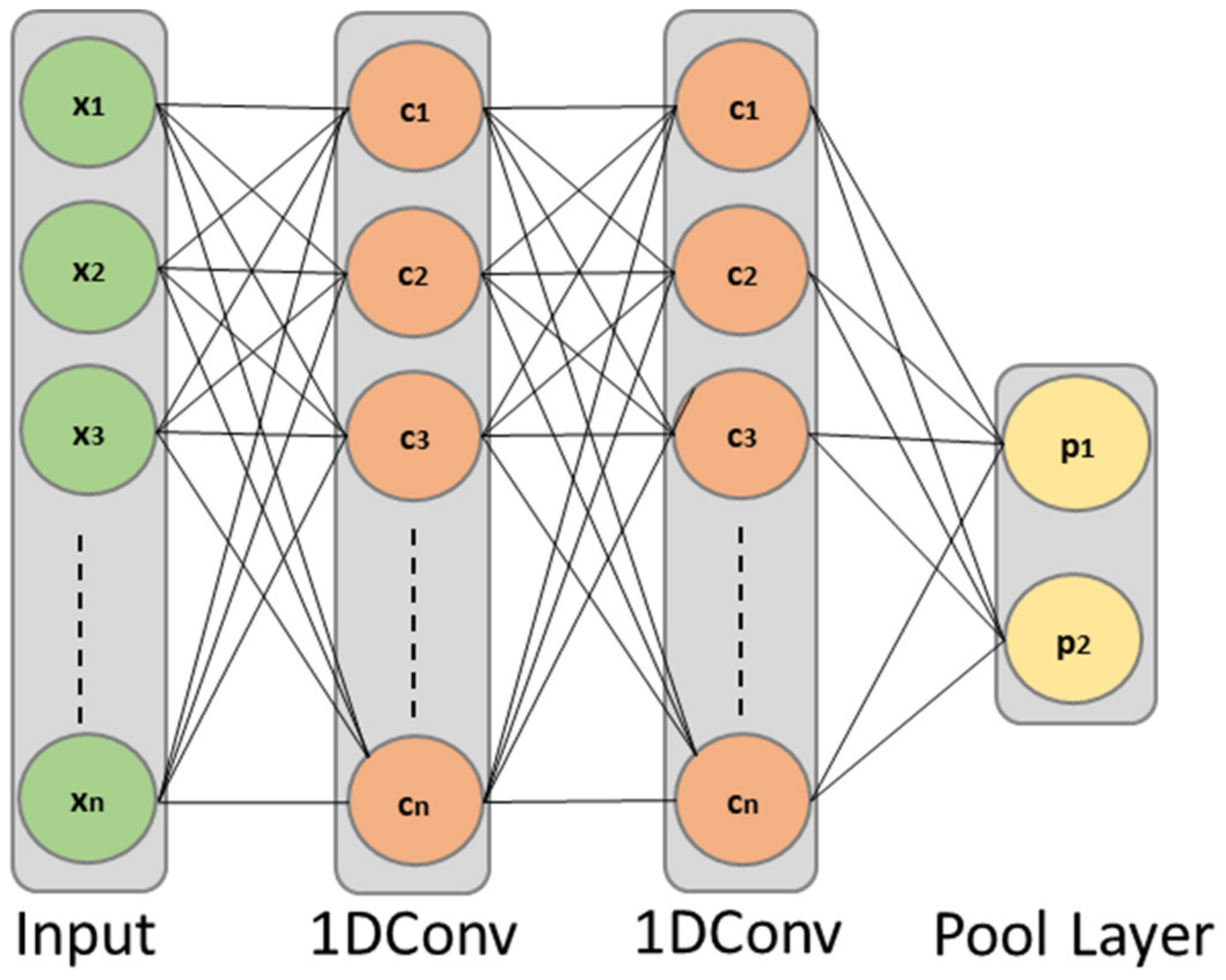
In computer vision, 2D CNN models have shown an encouraging performance on both image and video data such as facial expression analysis [52], action recognition [53], movie/video summarization [54], violence detection [55], etc. The 2D model accepts input in the two-dimension format in which pixels of images with color channels are processed simultaneously known as feature learning [56]. The same process can be applied in 1D sequential data but with variations in the input. Therefore, 1D CNNs are considered as an efficient approach for time series data to extract fixed-length feature vectors. In the case of non-linear tasks such as energy consumption prediction/forecasting, CNN utilizes the weight sharing concept that provides minimum error rate in terms of MSE [57]. In this study, we use two 1D CNN and pooling layers for efficient encoding the sequences of energy data, as shown in Figure 4, where x1, x2, x3, … xn represent the input data, c1, c2, c3, … cn, indicate the 1D convolutional layers for generating feature maps, and p1, p2 illustrate pooling layers that are employed to reduce the feature maps dimensions.

4. Experimental Evaluation

This section provides details for the evaluation of the proposed model, including dataset description, evaluation metrics, ablation study, time complexity comparison, and comparative analysis with state-of-the-art models. Note that we use different resolutions of the data such as minutely, hourly, daily, and weekly for the comparative analysis of the proposed models. However, for comparison with state-of-the-art, we only consider the commonly used resolution, i.e., hourly. We implemented the proposed approach in Keras (2.3.1) library with TensorFlow (1.13.1) as a backend using python language (3.5.5). Besides, Windows 10 operating system with GeForce RTX 2070 SUPER is used to train the model for 50 epochs, using batch size 32 and optimization algorithm (Adam) with an initial learning rate of 0.001.

4.1. Datasets Description

The proposed models are evaluated on two publicly available datasets. The household power energy consumption prediction dataset [58] is obtained from the University of California, Irvine (UCI) repository, which is originally recorded during the years 2006–2010 from residential buildings in France. This dataset is available with one-minute samples, consisting of 2,075,259 instances with 1.25% of missing values. Similarly, the second dataset [17] is collected from the commercial buildings in South Korea consisting of 99,372 instances with 15-min samples. First, both datasets are passed from preprocessing step for data cleansing and normalization. Next, these datasets are arranged in four samples, i.e., minutely, hourly, daily, and weekly for both short- and long-term predictions. The common attributes along with respected units for both datasets are listed in

Table 1. Common attributes, units, and their description of the datasets used for the evaluation of the proposed model.

Attribute	Unit	Description
Date	DD/MM/YYYY	The most important feature to indicate consumption of the power at specific days and months, where DD ranges from 1 to 31, MM from 1 to 12, and YYYY from 2006 to 2010.
Time	HH/MM/SS	This feature is mostly used for short-term prediction, i.e., minutely and hourly, where HH ranges from 0 to 23, MM and SS from 1 to 60.
Global Active Power (GAP)	K-W	This feature contains per minute data of total household average data.
Global Reactive Power (GRP)	K-W	Each minute data of overall building average power reactive.
Voltage (V)	Volts	Per-minute voltage level.
Global Intensity (GI)	Amp	Overall average power intensity per minute.

, while statistics of both datasets are provided in

Table 2. Statistics of the datasets including max, min, standard deviation, and average values for the used feature.

Dataset	Household Dataset				Commercial Dataset
Features	GAP	GRP	Voltage	GI	GAP	GRP
Min	0.076	0.000	223.20	0.200	0.000	0.000
Max	11.122	1.390	254.150	48.400	7.443	2.541
S.D.	1.055	0.113	3.239	4.435	0.564	0.114
Ave	1.089	0.124	240.844	4.618	0.405	0.071

.

4.2. Evaluation Metrics

Four common evaluation metrics are used to evaluate the proposed models and comparative analysis. These four evaluation matrices are mean squared error (MSE), mean absolute error (MAE), root mean square error (RMSE), and mean absolute percentage error (MAPE), which are mathematically expressed in Equations (11)–(14), respectively. MSE is basically the average squared difference between estimated and actual values, which always gives a non-negative value, with values closer to zero considered better, while RMSE is the square root of MSE. MAE measures the errors between paired observations expressing the same phenomenon, while MAPE is a common measure to calculate a forecast error in time series analysis that reflects the percentage variation between the forecasted variables.

$$\mathrm{MSE}=\frac{1}{n}{\displaystyle \sum }_{i=1}^n{\left(y_i-{\hat{y}}_i\right)}^2$$

(11)

$$\mathrm{MAE}=\frac{1}{n}{\displaystyle \sum }_{i=1}^n\left|y_i-{\hat{y}}_i\right|$$

(12)

$$\mathrm{RMSE}=\sqrt{\frac{1}{n}{\displaystyle \sum }_{i=1}^n{\left(y_i-{\hat{y}}_i\right)}^2}$$

(13)

$$\mathrm{MAPE}=\frac{1}{n}{\displaystyle \sum }_{i=1}^n|\frac{y_i-{\hat{y}}_i}{{\hat{y}}_i}|\times 100$$

(14)

where y and ŷ are the predicted and actual values, respectively.

4.3. Comparison Based on Sequential Learning Models via Hold-Out Method

To evaluate the sequence learning models for short- and long-term prediction, we conducted experiments for different resolutions of the data, i.e., minutely, hourly, daily, and weekly.

Table 3. Performance of the proposed models on the minutely resolution.

Models	Household Dataset				Commercial Dataset
	MSE	RMSE	MAE	MAPE (%)	MSE	RMSE	MAE	MAPE (%)
BiLSTM	0.745	0.863	0.625	50.50	0.855	0.925	0.522	51.3
ED–BiLSTM	0.525	0.724	0.515	40.55	0.624	0.789	0.415	35.34
CNN–BiLSTM	0.365	0.604	0.435	33.55	0.453	0.673	0.358	33.25
ConvLSTM–BiLSTM	0.035	0.187	0.075	30.75	0.025	0.158	0.055	28.55

represents the results based on the minute resolution, in which ConvLSTM-BiLSTM obtained the least error rate for both datasets. The least error is indicated in bold, and the runner-up is represented by underlined text. For the Household Dataset, ConvLSTM–BiLSTM obtained 0.035%, 0.187%, 0.075%, and 30.75% error rates for MSE, RMSE, MAE and MAPE, respectively. On the other hand, the results for the Commercial Dataset are slightly better than the Household Dataset with 0.025%, 0.158%, 0.055%, and 28.55% values for MSE, RMSE, MAE, and MAPE, respectively. The runner-up model for each dataset is CNN–BiLSTM. Hence, it is evident that features extracted from ConvLSTM perform better than CNN.

Similarly,

Table 4. Performance of the proposed models on the hourly resolution.

Models	Household Dataset				Commercial Dataset
	MSE	RMSE	MAE	MAPE (%)	MSE	RMSE	MAE	MAPE (%)
BiLSTM	0.505	0.711	0.515	40.55	0.305	0.552	0.414	41.22
ED–BiLSTM	0.405	0.636	0.425	35.45	0.225	0.474	0.426	36.48
CNN–BiLSTM	0.305	0.552	0.315	31.45	0.205	0.452	0.416	32.44
ConvLSTM–BiLSTM	0.105	0.324	0.311	30.05	0.115	0.339	0.333	38.06

represents the results based on the hourly resolution; here, also the ConvLSTM–BiLSTM obtained the least error rate for both datasets except MAPE (38.06%) for the Commercial Dataset. The CNN–BiLSTM model is found to be the second-best model, which beats ConvLSTM–BiLSTM model in MAPE (32.44%) values for the Commercial Dataset, while encoder–decoder–BiLSTM (ED–BiLSTM) obtained the second least error for MAPE (36.48%) for the Commercial Dataset. Overall, the results of ConvLSTM–BiLSTM with the hourly resolution are still better than the rest of the sequential learning models.

Next, the performance results of day resolution are presented in

Table 5. Performance of the proposed models on day resolution.

Models	Household Dataset				Commercial Dataset
	MSE	RMSE	MAE	MAPE (%)	MSE	RMSE	MAE	MAPE (%)
BiLSTM	0.225	0.474	0.285	40.15	0.335	0.425	0.344	35.33
ED–BiLSTM	0.155	0.393	0.255	35.25	0.255	0.505	0.312	30.55
CNN–BiLSTM	0.125	0.353	0.225	30.25	0.355	0.596	0.335	25.55
ConvLSTM–BiLSTM	0.035	0.187	0.175	18.35	0.025	0.158	0.145	20.45

. For all the metrics, ConvLSTM–BiLSTM obtained the least error rate in each dataset. For instance, for the Household Dataset, ConvLSTM–BiLSTM obtained 0.035, 0.187, 0.175, and 18.35 for MSE, RMSE, MAE, and MAPE, respectively, whereas CNN–BiLSTM obtained the second-least error on this dataset. Similarly, for the Commercial Dataset, ConvLSTM–BiLSTM still remains the best in terms of the least error rate, while the runner-up models are different for each metric. For instance, ED–BiLSTM obtained 0.255 and 0.312 for MSE and MAE, BiLSTM obtained 0.425 for RMSE, and CNN–BiLSTM obtained 25.55 for MAPE.

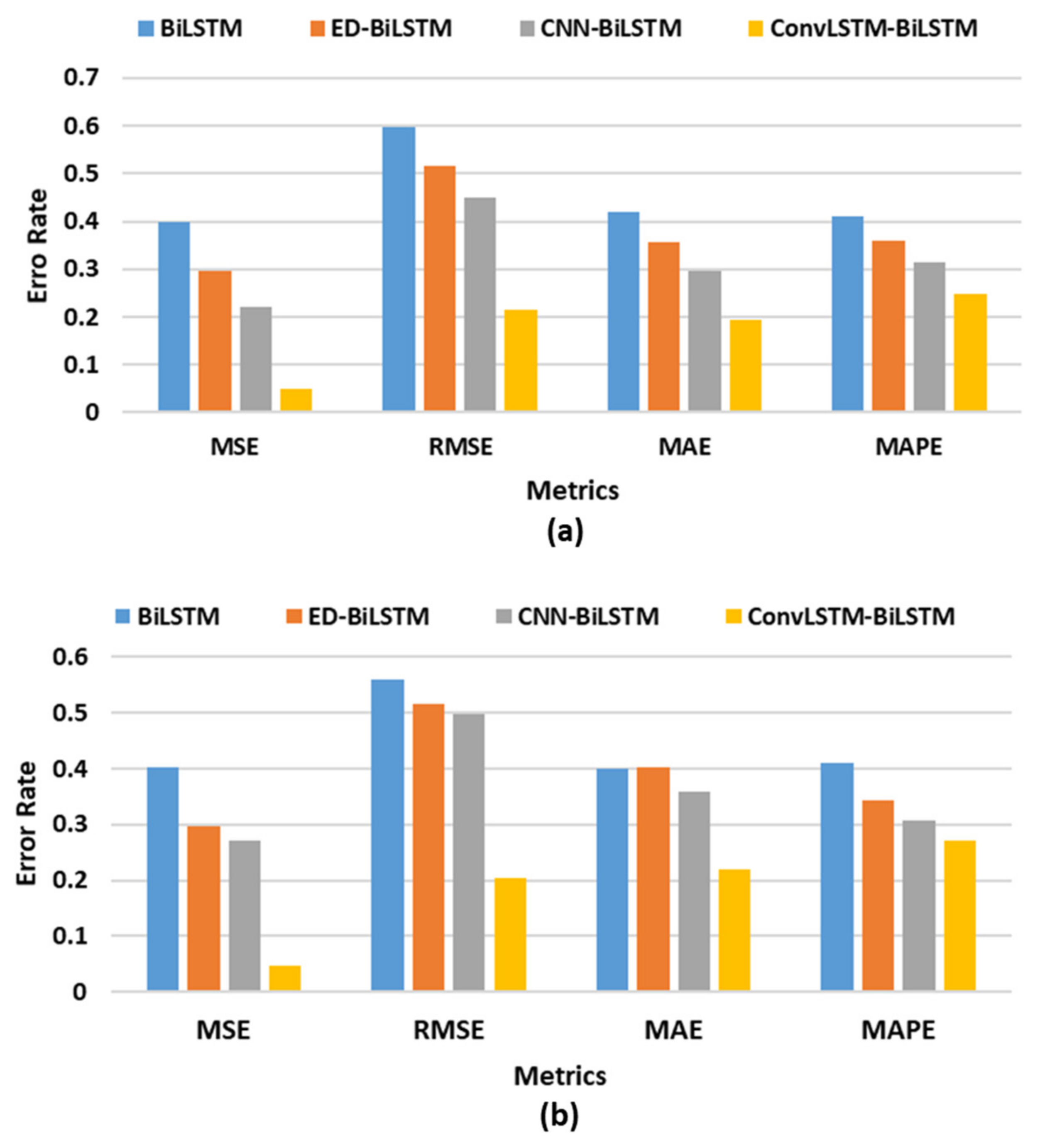
Finally, we performed experiments for long-term prediction by keeping the weekly resolution, as shown in

Table 6. Performance of the proposed models on the weekly resolution.

Models	Household Dataset				Commercial Dataset
	MSE	RMSE	MAE	MAPE (%)	MSE	RMSE	MAE	MAPE (%)
BiLSTM	0.115	0.339	0.255	33.55	0.112	0.334	0.324	36.45
ED–BiLSTM	0.095	0.308	0.235	32.34	0.085	0.292	0.254	35.43
CNN–BiLSTM	0.085	0.291	0.215	30.25	0.075	0.274	0.224	31.81
ConvLSTM–BiLSTM	0.028	0.167	0.155	20.15	0.025	0.158	0.143	20.91

. The best prediction model on the weekly dataset is also ConvLSTM–BiLSTM that obtains the least error rate for both datasets. For instance, for the Household Dataset, ConvLSTM–BiLSTM obtained 0.028, 0.167, 0.155, and 20.15 for MSE, RMSE, MAE and MAPE, respectively, and 0.025, 0.158, 0.143, and 20.91 for the Commercial Dataset. In contrast, the second-least error is obtained by CNN–BiLSTM. To summarize all the results in one graph, we calculated the average of each resolution (i.e., minutely, hourly, daily, and weekly), as illustrated in Figure 5. The MAPE value is ranged between zero and one instead of percentage for better representation. It is clear from Figure 5 that ConvLSTM–BiLSTM is leading in each dataset and metrics in terms of least error rate, followed by CNN–BiLSTM, ED–BiLSTM, and BiLSTM as runner up, third, and fourth place, respectively.

4.4. Comparison of the Sequential Learning Models Based on Cross-Validation Method

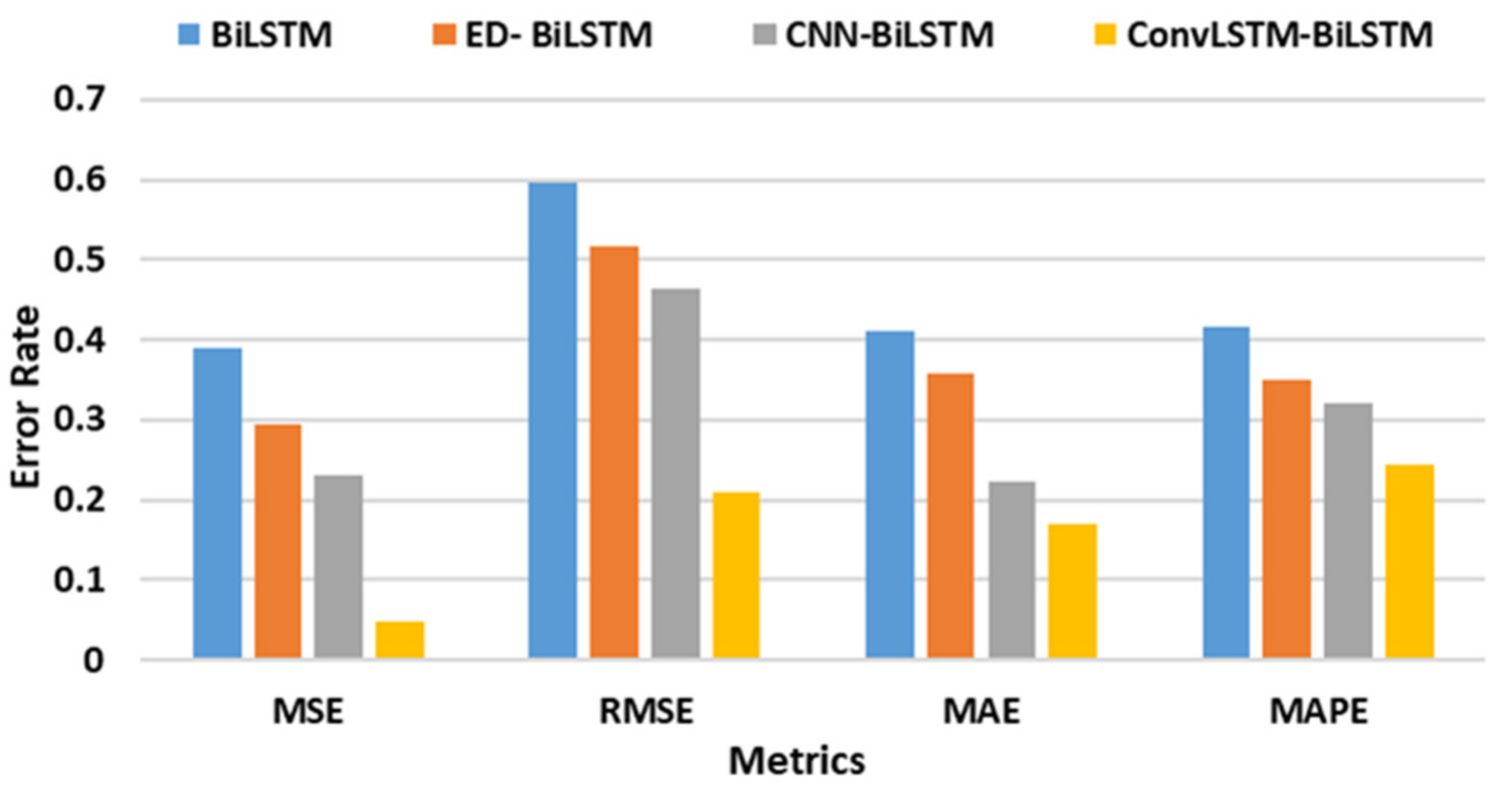
To validate the proposed model further in terms of learning and forecasting at the same time, we conducted experiments using a cross-validation method. In the cross-validation method, the overall dataset is divided into K equal segments or fold and K iterations for training and testing, which is conducted in such a way that each segment is kept for testing one by one, and the remaining K-1 segments are used for training. Finally, average accuracy is calculated over all iterations. In our case, we selected K = 10 (i.e., 10-fold validation) for the experiments over the household power energy prediction dataset [58].

Table 7. Performance of the proposed models using cross-validation method for various data resolutions.

Models	MSE	RMSE	MAE	MAPE (%)
	Minute Resolution
BiLSTM	0.697	0.834	0.593	49.87
ED–BiLSTM	0.518	0.719	0.512	40.12
CNN–BiLSTM	0.398	0.631	0.459	34.79
ConvLSTM–BiLSTM	0.031	0.176	0.072	29.14
Hour Resolution
BiLSTM	0.496	0.704	0.502	40.01
ED–BiLSTM	0.401	0.633	0.415	35.29
CNN–BiLSTM	0.301	0.548	0.312	31.19
ConvLSTM–BiLSTM	0.102	0.319	0.304	30.03
Day Resolution
BiLSTM	0.229	0.478	0.291	41.19
ED–BiLSTM	0.159	0.398	0.263	31.96
CNN–BiLSTM	0.121	0.347	0.221	30.19
ConvLSTM–BiLSTM	0.029	0.167	0.138	17.98
Week Resolution
BiLSTM	0.138	0.371	0.264	35.37
ED–BiLSTM	0.103	0.322	0.239	33.01
CNN–BiLSTM	0.108	0.328	0.223	31.73
ConvLSTM–BiLSTM	0.031	0.176	0.162	21.03

represents the overall results for different sequential models over various data resolutions. Here also, ConvLSTM–BiLSTM obtained the least error rates on each data resolution, compared to other sequential models, while CNN–BiLSTM remains the runner-up model, except for the weekly resolution. The ED–BiLSTM remains the runner-up for weekly resolution in MSE and RMSE metrics, obtaining 0.103 and 0.322 error rates, respectively. Hence, the reported results based on the cross-validation method provide evidence that ConvLSTM–BiLSTM is the most effective combination in terms of learning and forecasting among the other models. Figure 6 illustrates the average results of overall resolution for each model, in which the MAPE value is presented in the range of zero and one instead of percentage for better presentation.

4.5. Comparative Analysis Based on Time Complexity of the Sequential Models

This section presents the time complexity analysis between the sequential learning models proposed in this study over two different platforms, i.e., central processing unit (CPU) and graphics processing unit (GPU).

Table 8. Comparative analysis of the sequential models based on time complexity in seconds (s) over Household Dataset.

Models	CPU		GPU
	Training Time (s)	Testing Time (s)	Training Time (s)	Testing Time (s)
Day Resolution
BiLSTM	174.57	1.16	64.30	0.42
ED–BiLSTM	418.77	2.78	191.48	1.27
CNN–BiLSTM	192.07	1.28	83.20	0.55
ConvLSTM–BiLSTM	217.49	1.44	108.52	0.72
Week Resolution
BiLSTM	20.38	0.13	07.37	0.04
ED–BiLSTM	48.29	0.32	21.57	0.14
CNN–BiLSTM	29.74	0.19	11.12	0.07
ConvLSTM–BiLSTM	41.43	0.27	17.14	0.11

represents the time complexity of the training and testing sessions in seconds (s) over the Household Dataset. For this comparison, we considered two data resolutions (i.e., day and week), through which it can be analyzed that low-resolution data comparatively have low-time complexity and vice-versa. It is clear from Table 8 that BiLSTM achieved the overall lowest, while ED–BiLSTM achieved the maximum time complexity. However, ConvLSTM–BiLSTM achieved the best trade-off between time complexity and accuracy.

4.6. Comparative Analysis with State-of-the-Art Models

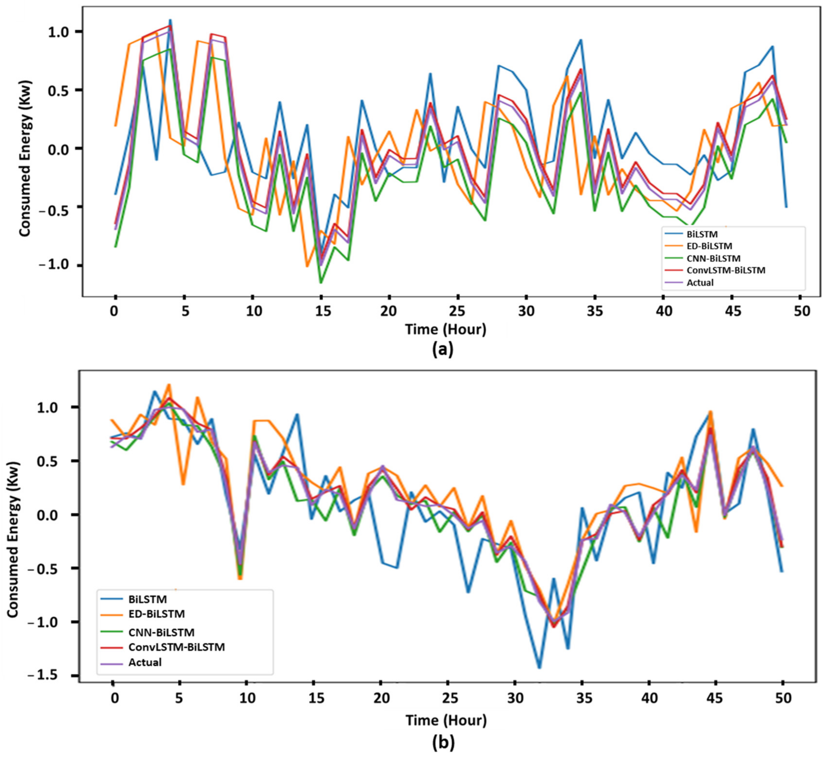
This section presents a comparative analysis of the proposed prediction model with seven recent state-of-the-art hybrid models based on hourly sampled data of the Household Dataset, as shown in

Table 9. Comparative analysis of the proposed model with state-of-the-art models based on hourly data resolution of Household Dataset.

Method	Strategy/Models	Error Metrics
		MSE	RMSE	MAE	MAPE (%)
Kim and Cho [23]	CNN–LSTM	0.37	0.61	0.34	34.48
Kim and Cho [18]	CNN–AE	0.38	-	0.39	-
Ullah et al. [26]	CNN–MultiLayer–BiLSTM	0.31	0.56	0.34	29.10
Le et al. [25]	CNN–BiLSTM	0.29	0.54	0.39	50.09
Khan et al. [17]	CNN–LSTM–AE	0.19	0.47	0.31	-
Sajjad et al. [28]	CNN–GRU	0.22	0.47	0.33	-
Khan et al. [59]	CNN–MB–GRU	0.18	0.42	0.29	-
Proposed	ConvLSTM–BiLSTM	0.10	0.32	0.31	30.05

. All the methods in comparison extract features using simple CNN and then forward the extracted features to different sequential learning models for energy consumption predictions. For instance, LSTM [23], auto encoder (AE) [18], Multi-layer Bidirectional LSTM [26], Bidirectional LSTM [25], LSTM followed by AE [17], GRU [28], and CNN with multilayer bidirectional gated recurrent unit (CNN–MB–GRU) [59]. For this comparison, we select the best-proposed model from Section 4.3, i.e., ConvLSTM–BiLSTM, which uses ConvLSTM as an encoder and bidirectional LSTM as a decoder. The proposed model outperforms state-of-the-art models in MSE and RMSE with the least error rate of 0.10 and 0.32, respectively. The proposed model reduced the error rate up to 0.08 and 0.1 points compared to the runner-up model CNN–MB–GRU [59] with MSE and RMSE values of 0.18 and 0.42, respectively. However, the least error rate for MAE is achieved by CNN–MB–GRU [59] with 0.29, while the proposed and CNN–LSTM–AE models remain runner up with a difference of 0.02. The proposed model achieved 30.05 error rate for MAPE metrics and remains runner up with a very little difference. The least error rate is achieved by CNN–MultiLayer–BiLSTM [26] with 29.10 and the difference with proposed model is only 0.95. Hence, the overall results demonstrate the superiority of the proposed model over state-of-the-art based on Household Dataset. Lastly, Figure 7 illustrates the prediction results of the proposed sequential learning models on hourly resolution data for both datasets.

5. Conclusions

In this paper, we provided a comparative analysis of various sequential learning models and selected the optimum one as the proposed model after extensive experimental findings. The proposed hybrid architecture for energy prediction is developed by integrating ConvLSTM and BiLSTM models. In detail, the proposed framework consisted of three main steps. First, the preprocessing step is applied to the input data for data cleansing such as normalization and missing values adjustment. Next, the preprocessed data are forwarded to the proposed hybrid model for training, in which ConvLSTM is used to extract and encode the spatial characteristics of the data, while BiLSTM is used to decode and learn the sequential patterns. Finally, the models are tested for both short- and long-term predictions using four resolutions, i.e., minutely, hourly, daily, and weekly, based on two datasets. In the comparative analysis, the proposed model achieved the least error rates against recent state-of-the-art energy prediction models. In the future, we aim to develop efficient prediction models that can be deployed over resource-constrained devices for smart metering and smart home appliances’ energy management.

References

- Elattar, E.E.; Sabiha, N.A.; Alsharef, M.; Metwaly, M.K.; Abd-Elhady, A.M.; Taha, I.B. Short term electric load forecasting using hybrid algorithm for smart cities. Appl. Intell. 2020, 50, 1–21. [Google Scholar] [CrossRef]
- Han, T.; Muhammad, K.; Hussain, T.; Lloret, J.; Baik, S.W. An Efficient Deep Learning Framework for Intelligent Energy Management in IoT Networks. IEEE Internet Things J. 2020, 8, 3170–3179. [Google Scholar] [CrossRef]
- Chen, S.; Wen, H.; Wu, J.; Lei, W.; Hou, W.; Liu, W.; Xu, A.; Jiang, Y. Internet of Things based smart grids supported by intelligent edge computing. IEEE Access 2019, 7, 74089–74102. [Google Scholar] [CrossRef]
- Carvallo, J.P.; Larsen, P.H.; Sanstad, A.H.; Goldman, C.A. Long term load forecasting accuracy in electric utility integrated resource planning. Energy Policy 2018, 119, 410–422. [Google Scholar] [CrossRef] [Green Version]
- Mashhadi, A.R.; Behdad, S. Discriminant effects of consumer electronics use-phase attributes on household energy prediction. Energy Policy 2018, 118, 346–355. [Google Scholar] [CrossRef] [Green Version]
- Hapka, A.R.; Bunn, D.W.; Farmer, E.D. Comparative Models for Electrical Load Forecasting; Wiley: Ulster, UK; Elsevier: Amsterdam, The Netherlands, 1986; p. 232. [Google Scholar]
- Rodger, J.A. A fuzzy nearest neighbor neural network statistical model for predicting demand for natural gas and energy cost savings in public buildings. Expert Syst. Appl. 2014, 41, 1813–1829. [Google Scholar] [CrossRef]
- Chalal, M.L.; Benachir, M.; White, M.; Shrahily, R. Energy planning and forecasting approaches for supporting physical improvement strategies in the building sector: A review. Renew. Sustain. Energy Rev. 2016, 64, 761–776. [Google Scholar] [CrossRef] [Green Version]
- Irtija, N.; Sangoleye, F.; Tsiropoulou, E.E. Contract-Theoretic Demand Response Management in Smart Grid Systems. IEEE Access 2020, 8, 184976–184987. [Google Scholar] [CrossRef]
- Swan, L.G.; Ugursal, V.I. Modeling of end-use energy consumption in the residential sector: A review of modeling techniques. Renew. Sustain. Energy Rev. 2009, 13, 1819–1835. [Google Scholar] [CrossRef]
- Amasyali, K.; El-Gohary, N.M. A review of data-driven building energy consumption prediction studies. Renew. Sustain. Energy Rev. 2018, 81, 1192–1205. [Google Scholar] [CrossRef]
- Ullah, A.; Ahmad, J.; Muhammad, K.; Sajjad, M.; Baik, S.W. Action recognition in video sequences using deep bi-directional LSTM with CNN features. IEEE Access 2017, 6, 1155–1166. [Google Scholar] [CrossRef]
- Song, W.; Zheng, J.; Wu, Y.; Chen, C.; Liu, F. Discriminative feature extraction for video person re-identification via multi-task network. Appl. Intell. 2020, 51, 788–803. [Google Scholar] [CrossRef]
- Wang, D.; Xin, J. Emergent spatio-temporal multimodal learning using a developmental network. Appl. Intell. 2019, 49, 1306–1323. [Google Scholar] [CrossRef]
- Wang, T.; Liu, L.; Liu, N.; Zhang, H.; Zhang, L.; Feng, S. A multi-label text classification method via dynamic semantic representation model and deep neural network. Appl. Intell. 2020, 50, 2339–2351. [Google Scholar] [CrossRef]
- Xu, W.; Peng, H.; Zeng, X.; Zhou, F.; Tian, X.; Peng, X. A hybrid modelling method for time series forecasting based on a linear regression model and deep learning. Appl. Intell. 2019, 49, 3002–3015. [Google Scholar] [CrossRef]
- Khan, Z.A.; Hussain, T.; Ullah, A.; Rho, S.; Lee, M.; Baik, S.W. Towards Efficient Electricity Forecasting in Residential and Commercial Buildings: A Novel Hybrid CNN with a LSTM-AE based Framework. Sensors 2020, 20, 1399. [Google Scholar] [CrossRef] [PubMed] [Green Version]
- Kim, J.-Y.; Cho, S.-B. Electric energy consumption prediction by deep learning with state explainable autoencoder. Energies 2019, 12, 739. [Google Scholar] [CrossRef] [Green Version]
- Fallah, S.N.; Deo, R.C.; Shojafar, M.; Conti, M.; Shamshirband, S. Computational intelligence approaches for energy load forecasting in smart energy management grids: State of the art, future challenges, and research directions. Energies 2018, 11, 596. [Google Scholar] [CrossRef] [Green Version]
- Hussain, T.; Ullah, F.U.M.; Muhammad, K.; Rho, S.; Ullah, A.; Hwang, E.; Moon, J.; Baik, S.W. Smart and Intelligent Energy Monitoring Systems: A Comprehensive Literature Survey and Future Research Guidelines. Int. J. Energy Res. 2021, 45, 3590–3614. [Google Scholar] [CrossRef]
- Kong, W.; Dong, Z.Y.; Hill, D.J.; Luo, F.; Xu, Y. Short-term residential load forecasting based on resident behaviour learning. IEEE Trans. Power Syst. 2017, 33, 1087–1088. [Google Scholar] [CrossRef]
- Almalaq, A.; Zhang, J.J. Evolutionary deep learning-based energy consumption prediction for buildings. IEEE Access 2018, 7, 1520–1531. [Google Scholar] [CrossRef]
- Kim, T.-Y.; Cho, S.-B. Predicting residential energy consumption using CNN-LSTM neural networks. Energy 2019, 182, 72–81. [Google Scholar] [CrossRef]
- Zhou, C.; Sun, C.; Liu, Z.; Lau, F. A C-LSTM neural network for text classification. arXiv 2015, arXiv:1511.08630. [Google Scholar]
- Ullah, F.U.M.; Ullah, A.; Haq, I.U.; Rho, S.; Baik, S.W. Short-Term Prediction of Residential Power Energy Consumption via CNN and Multilayer Bi-directional LSTM Networks. IEEE Access 2019, 8, 123369–123380. [Google Scholar] [CrossRef]
- Wen, L.; Zhou, K.; Yang, S.; Lu, X. Optimal load dispatch of community microgrid with deep learning based solar power and load forecasting. Energy 2019, 171, 1053–1065. [Google Scholar] [CrossRef]
- Sajjad, M.; Khan, Z.A.; Ullah, A.; Hussain, T.; Ullah, W.; Lee, M.Y.; Baik, S.W. A novel CNN-GRU-based hybrid approach for short-term residential load forecasting. IEEE Access 2020, 8, 143759–143768. [Google Scholar] [CrossRef]
- Rahman, H.; Selvarasan, I.; Begum, A.J. Short-Term Forecasting of Total Energy Consumption for India-A Black Box Based Approach. Energies 2018, 11, 3442. [Google Scholar] [CrossRef] [Green Version]
- Jain, R.K.; Smith, K.M.; Culligan, P.J.; Taylor, J.E. Forecasting energy consumption of multi-family residential buildings using support vector regression: Investigating the impact of temporal and spatial monitoring granularity on performance accuracy. Appl. Energy 2014, 123, 168–178. [Google Scholar] [CrossRef]
- Zheng, H.; Yuan, J.; Chen, L. Short-term load forecasting using EMD-LSTM neural networks with a Xgboost algorithm for feature importance evaluation. Energies 2017, 10, 1168. [Google Scholar] [CrossRef] [Green Version]
- Chujai, P.; Kerdprasop, N.; Kerdprasop, K. Time series analysis of household electric consumption with ARIMA and ARMA models. In Proceedings of the International MultiConference of Engineers and Computer Scientists, Hong Kong, China, 21–23 October 2020; pp. 295–300. [Google Scholar]
- Muralitharan, K.; Sakthivel, R.; Vishnuvarthan, R. Neural network based optimization approach for energy demand prediction in smart grid. Neurocomputing 2018, 273, 199–208. [Google Scholar] [CrossRef]
- Aslam, S.; Khalid, A.; Javaid, N. Towards efficient energy management in smart grids considering microgrids with day-ahead energy forecasting. Electr. Power Syst. Res. 2020, 182, 106232. [Google Scholar] [CrossRef]
- Bourhnane, S.; Abid, M.R.; Lghoul, R.; Zine-Dine, K.; Elkamoun, N.; Benhaddou, D. Machine learning for energy consumption prediction and scheduling in smart buildings. SN Appl. Sci. 2020, 2, 297. [Google Scholar] [CrossRef] [Green Version]
- Somu, N.; MR, G.R.; Ramamritham, K. A hybrid model for building energy consumption forecasting using long short term memory networks. Appl. Energy 2020, 261, 114131. [Google Scholar] [CrossRef]
- Shao, M.; Wang, X.; Bu, Z.; Chen, X.; Wang, Y. Prediction of energy consumption in hotel buildings via support vector machines. Sustain. Cities Soc. 2020, 57, 102128. [Google Scholar] [CrossRef]
- Ruiz, L.; Pegalajar, M.; Arcucci, R.; Molina-Solana, M. A time-series clustering methodology for knowledge extraction in energy consumption data. Expert Syst. Appl. 2020, 160, 113731. [Google Scholar] [CrossRef]
- Fang, X.; Gong, G.; Li, G.; Chun, L.; Li, W.; Peng, P. A hybrid deep transfer learning strategy for short term cross-building energy prediction. Energy 2020, 215, 119208. [Google Scholar] [CrossRef]
- Hu, H.; Wang, L.; Lv, S.-X. Forecasting energy consumption and wind power generation using deep echo state network. Renew. Energy 2020, 154, 598–613. [Google Scholar] [CrossRef]
- Wen, L.; Zhou, K.; Yang, S. Load demand forecasting of residential buildings using a deep learning model. Electr. Power Syst. Res. 2020, 179, 106073. [Google Scholar] [CrossRef]
- Zhang, Z.; Lv, Z.; Gan, C.; Zhu, Q. Human action recognition using convolutional LSTM and fully-connected LSTM with different attentions. Neurocomputing 2020, 410, 304–316. [Google Scholar] [CrossRef]
- Xingjian, S.; Chen, Z.; Wang, H.; Yeung, D.-Y.; Wong, W.-K.; Woo, W.-C. Convolutional LSTM network: A machine learning approach for precipitation nowcasting. In Proceedings of the Advances in Neural Information Processing Systems, NIPS, Montreal, QC, Canada, 7–10 December 2015; pp. 802–810. [Google Scholar]
- Sutskever, I.; Vinyals, O.; Le, Q.V. Sequence to sequence learning with neural networks. In Advances in Neural Information Processing Systems; MIT: Cambridge, MA, USA, 2014; pp. 3104–3112. [Google Scholar]
- Srivastava, N.; Mansimov, E.; Salakhudinov, R. Unsupervised learning of video representations using lstms. In Proceedings of the International Conference on Machine Learning; ICML: Lille, France, 2015; pp. 843–852. [Google Scholar]
- Mikolov, T.; Karafiát, M.; Burget, L.; Cernocky, J.; Khudanpur, S. Recurrent neural network based language model. In Proceedings of the Eleventh Annual Conference of the International Speech Communication Association, Dresden, Germany, 6–10 September 2015. [Google Scholar]
- Sajjad, M.; Khan, S.U.; Khan, N.; Haq, I.U.; Ullah, A.; Lee, M.Y.; Baik, S.W. Towards Efficient Building Designing: Heating and Cooling Load Prediction via Multi-Output Model. Sensors 2020, 20, 6419. [Google Scholar] [CrossRef]
- Bengio, Y.; Simard, P.; Frasconi, P. Learning long-term dependencies with gradient descent is difficult. IEEE Trans. Neural Netw. 1994, 5, 157–166. [Google Scholar] [CrossRef] [PubMed]
- Hochreiter, S.; Schmidhuber, J. Long short-term memory. Neural Comput. 1997, 9, 1735–1780. [Google Scholar] [CrossRef]
- Schuster, M.; Paliwal, K.K. Bidirectional recurrent neural networks. IEEE Trans. Signal. Process. 1997, 45, 2673–2681. [Google Scholar] [CrossRef] [Green Version]
- Khan, N.; Ullah, F.U.M.; Ullah, A.; Lee, M.Y.; Baik, S.W. Batteries State of Health Estimation via Efficient Neural Networks with Multiple Channel Charging Profiles. IEEE Access 2020, 9, 7797–7813. [Google Scholar] [CrossRef]
- Sajjad, M.; Zahir, S.; Ullah, A.; Akhtar, Z.; Muhammad, K. Human Behavior Understanding in Big Multimedia Data Using CNN based Facial Expression Recognition. Mob. Netw. Appl. 2019, 25, 1611–1621. [Google Scholar] [CrossRef]
- Ullah, A.; Muhammad, K.; Hussain, T.; Lee, M.; Baik, S.W. Deep LSTM-Based Sequence Learning Approaches for Action and Activity Recognition. In Deep Learning in Computer Vision; CRC Press: Boca Raton, FL, USA, 2020; p. 127. [Google Scholar]
- Haq, I.U.; Ullah, A.; Muhammad, K.; Lee, M.Y.; Baik, S.W. Personalized movie summarization using deep cnn-assisted facial expression recognition. Complexity 2019, 2019, 1–10. [Google Scholar] [CrossRef] [Green Version]
- Khan, S.U.; Haq, I.U.; Rho, S.; Baik, S.W.; Lee, M.Y. Cover the violence: A novel Deep-Learning-Based approach towards violence-detection in movies. Appl. Sci. 2019, 9, 4963. [Google Scholar] [CrossRef] [Green Version]
- Khan, N.; Ullah, A.; Haq, I.U.; Menon, V.G.; Baik, S.W. SD-Net: Understanding overcrowded scenes in real-time via an efficient dilated convolutional neural network. J. Real-Time Image Process. 2020, 1–15. [Google Scholar] [CrossRef]
- Qiu, Z.; Chen, J.; Zhao, Y.; Zhu, S.; He, Y.; Zhang, C. Variety identification of single rice seed using hyperspectral imaging combined with convolutional neural network. Appl. Sci. 2018, 8, 212. [Google Scholar] [CrossRef] [Green Version]
- UCI. Individual Household Electric Power Consumption Data Set; UCI: Irvine, CA, USA, 2012. [Google Scholar]
- Le, T.; Vo, M.T.; Vo, B.; Hwang, E.; Rho, S.; Baik, S.W. Improving Electr. energy consumption prediction using CNN and Bi-LSTM. Appl. Sci. 2019, 9, 4237. [Google Scholar] [CrossRef] [Green Version]
- Khan, Z.A.; Ullah, A.; Ullah, W.; Rho, S.; Lee, M.; Baik, S.W. Electrical Energy Prediction in Residential Buildings for Short-Term Horizons Using Hybrid Deep Learning Strategy. Appl. Sci. 2020, 10, 8634. [Google Scholar] [CrossRef]
Figure 1.
The proposed framework for power energy consumption prediction comprises three main steps—Step 1: the smart microgrids generate power energy and supply it to residential buildings/smart factories where smart meters measure the consumed energy; Step 2: smart meters’ data are significantly influenced by environmental factors that generate abnormalities; therefore, data cleansing schemes are applied as preprocessing step; and Step 3: train the model with refined data in which ConvLSTM and BiLSTM layers are used for encoding and decoding the numerous resolutions of data to obtain a minimum error rate.
Figure 2.
Household Dataset representation (a) before and (b) after the preprocessing step.
Figure 3.
The internal architecture of (a) fully connected long short-term memory (LSTM) and (b) convolutional long short-term memory (ConvLSTM).