Mathematical Modeling of Japanese Encephalitis under Aquatic Environmental Effects

Abstract

We propose a mathematical model for the spread of Japanese encephalitis with emphasis on the environmental effects on the aquatic phase of mosquitoes. The model is shown to be biologically well-posed and to have a biologically and ecologically meaningful disease-free equilibrium point. Local stability is analyzed in terms of the basic reproduction number and numerical simulations presented and discussed.

1. Introduction

Japanese encephalitis (JE) is a mosquito-borne disease transmitted to humans through the bite of an infected mosquito, particularly a Culex tritaeniorhynchus mosquito. The mosquitoes breed where there is abundant water in rural agricultural areas, such as rice paddies, and become infected by feeding on vertebrate hosts (primarily pigs and wading birds) infected with the Japanese encephalitis virus. The virus is maintained in a cycle between those vertebrate animals and mosquitoes. Humans are dead-end hosts since they usually do not develop high enough concentrations of JE virus in their bloodstreams to infect feeding mosquitoes [1].

Human infection occasionally causes brain inflammation with symptoms such as headache, vomiting, fever, confusion, and epileptic seizure. There is an estimate of about 68,000 clinical cases of occurrences with nearly 17,000 deaths every year in Asian countries [2].

The first case of Japanese encephalitis viral disease was documented in 1871 in Japan, but the virus itself was first isolated in 1935 and has subsequently been found across most of Asia. There is uncertainty on the origin of the name of that virus; however, phylogenetic comparisons with other flaviviruses suggest that it evolved from an African ancestral virus, perhaps as recently as a few centuries ago (see [3] and references therein). Note that, despite its name, Japanese encephalitis is now relatively rare in Japan as a result of a mass immunization program.

Mathematical modeling in the field of biosciences is a subject of strong current research (see, e.g., [4,5,6]). One of the first mathematical models for the spread of JE was proposed and analyzed in 2009 in [7]. Later, in 2012, a study of the impact of media on the spreading and control of JE was carried out [8], while in 2016, several measures to control JE, such as vaccination, medicine, and insecticide, were investigated through optimal control and Pontryagin’s maximum principle. The state of the art of mathematical modeling and analysis of JE seems to be found in recent papers [9,10] from 2018. In [9], a mathematical model of transmission of JE, described by a system of eight ordinary differential equations, is proposed and studied. The main results are the basic reproduction number and a stability analysis around the interior equilibrium. The authors of [10] use mathematical modeling and likelihood-based inference techniques to try to explain the disappearance of JE human cases between 2006 and 2010 and its resurgence in 2011. Here, we propose a mathematical model for the spread of JE, incorporating environmental effects on the aquatic phase of mosquitoes as the primary source of reproduction.

The manuscript is organized as follows. In Section 2, we introduce the mathematical model. Then, in Section 3, the theoretical analysis of the model is investigated: the well-posedness of the model is proved (see Theorem 1), and the meaningful disease-free equilibrium and its local stability, in terms of the basic reproduction number, are analyzed in detail (see Theorem 2). Section 4 is then devoted to numerical simulations. We end with Section 5 of conclusions, where we also point out some possible directions of future research.

2. Model Formulation

In our mathematical model, we shall consider environmental factors within three different host populations: humans, mosquitoes, and vertebrate animals (pigs or wading birds) as the reservoir host. In fact, unhygienic environmental conditions may enhance the presence and growth of vectors (mosquitoes) populations, leading to fast spread of the disease. This is due to the discharge of various kinds of household and other wastes into the environment in residential areas of population, thus providing a very conducive environment for the growth of vectors [11,12]. Since that effect could not be modeled as epidemiological compartments, we use the same scheme as in [13,14] to handle that effect on the JE disease, namely [7]

$${\displaystyle \frac{dE\left(t\right)}{dt}=Q_0+\theta N\left(t\right)-{\theta }_{0}E\left(t\right),}$$

(1)

where E is the cumulative density of environmental discharges conducive to the growth rate of mosquitoes and animals. The cumulative density of environmental discharges due to human activities is given by $\theta$. There is also a constant influx given by $Q_0$, and ${\theta }_0$ is the depletion rate coefficient of the environmental discharges. In our model, $N\left(t\right)$ stands for the total human population, which is considered a varying function of time t.

As for the reservoir animal populations, we consider their dynamics, strongly related to infected animals. Thus, the reservoir population constitutes a “pool of infection” that is a primarily source of infections and can be modeled by a single state variable, as in the framework of viruses, having free living pathogens in the environment (see, e.g., [15,16,17] and references therein for diseases like cholera, typhoid, or yellow fever). Therefore, we consider a single state variable, denoted by $I_r$, to model this reservoir pool of infection:

$${\displaystyle \frac{d{I}_r\left(t\right)}{dt}=B{\beta }_{mr}\frac{I_m\left(t\right)}{N_m\left(t\right)}{I}_r\left(t\right)-\left({\mu }_{1r}+{\mu }_{2r}{I}_r\left(t\right)\right)I_r\left(t\right)-d_r{I}_r\left(t\right)+{\delta }_0{I}_r\left(t\right)E\left(t\right),}$$

(2)

where ${\displaystyle B{\beta }_{mr}\frac{I_m}{N_m}{I}_r\left(t\right)}$ represents the force of infection due to interaction with mosquitoes through biting; B is the average daily biting; ${\beta }_{mr}$ is the transmission coefficient from infected mosquitoes; $\frac{I_m}{N_m}$ is the fraction of infected mosquitoes; ${\mu }_{1r}$ is the natural death rate of animals; ${\mu }_{2r}$ is the density dependent death rate; $d_r$ is the death rate due to the disease; and ${\delta }_0$ is the per capita growth rate due to environmental discharges. Note that we are not interested in how the disease spreads to other animals. Our main goal is to study the transmission of infections from mosquitoes to humans as well as the related environmental effects.

The following assumptions are made in order to build the compartmental classes for mosquitoes and human populations:

• we do not consider immigration of infected humans;
• the human population is not constant (we consider a disease-induced death rate, due to fatality, of 25%);
• we assume that the coefficient of transmission of the virus is constant and does not vary with seasons, which is reasonable due to the short course of the disease;
• mosquitoes are assumed to be born susceptible.

Three epidemiological compartments are considered for the mosquito population—precisely, the aquatic phase, denoted by $A_m$, and including eggs, larva, and pupae stages; the susceptible mosquitoes, $S_m$; and the infected mosquitoes, $I_m$. There is also no resistant phase due to the short lifetime of mosquitoes:

$$\left\{\begin{array}{c}{\displaystyle \frac{d{A}_m\left(t\right)}{dt}=\psi \mathcal{(}1-\frac{A_m\left(t\right)}{K}\mathcal{)}(S_m\left(t\right)+I_m\left(t\right))-\left({\mu }_A+{\eta }_A\right)A_m\left(t\right)+\delta E\left(t\right)A_m\left(t\right),}\hfill \\ {\displaystyle \frac{d{S}_m\left(t\right)}{dt}={\eta }_A{A}_m\left(t\right)-B{\beta }_{rm}{I}_r\left(t\right)S_m\left(t\right)-{\mu }_m{S}_m\left(t\right),}\hfill \\ {\displaystyle \frac{d{I}_m}{dt}=B{\beta }_{rm}{I}_r\left(t\right)S_m\left(t\right)-{\mu }_m{I}_m\left(t\right),}\hfill \end{array}\right.$$

(3)

where parameter ${\beta }_{rm}$ represents the transmission probability from infected animals $I_r$ (per bite), B is the average daily biting, $\psi$ stands for the number of eggs at each deposit per capita (per day), ${\mu }_A$ is the natural mortality rate of larvae (per day), ${\eta }_A$ is the maturation rate from larvae to adult (per day), and $\delta$ is the per capita growth rate in the level of aquatic phase due to conducive environmental discharge. Here, $\frac{1}{{\mu }_m}$ denotes the average lifespan of adult mosquitoes (in days), and K is the maximal capacity of larvae. We denote by $N_m$ the total adult mosquito populations at each instant of time t, being defined by $N_m\left(t\right)=S_m\left(t\right)+I_m\left(t\right)$ and with its dynamics satisfying the differential equation

$${\displaystyle \frac{d{N}_m\left(t\right)}{dt}={\eta }_A{A}_m\left(t\right)-{\mu }_m{N}_m.}$$

The total human population, given by function $N\left(t\right)$, is subdivided into two mutually exclusive compartments, according to the disease status, namely susceptible individuals, S, and infected individuals, I. We do not consider a recovery state since there is no adequate treatment for the JE disease and no person-to-person infection exists:

$$\left\{\begin{array}{c}{\displaystyle \frac{dN\left(t\right)}{dt}={\mathsf{\Lambda }}_h-{\mu }_{h}N\left(t\right)-d_{h}I\left(t\right),}\hfill \\ {\displaystyle \frac{dS\left(t\right)}{dt}={\mathsf{\Lambda }}_h-\left(B{\beta }_{mh}\frac{I_m\left(t\right)}{N_m\left(t\right)}\right)S\left(t\right)-{\mu }_{h}S\left(t\right)+{\nu }_{h}I\left(t\right),}\hfill \\ {\displaystyle \frac{dI\left(t\right)}{dt}=\left(B{\beta }_{mh}\frac{I_m\left(t\right)}{N_m\left(t\right)}\right)S\left(t\right)-{\mu }_{h}I\left(t\right)-{\nu }_{h}I\left(t\right)-d_{h}I\left(t\right),}\hfill \end{array}\right.$$

(4)

where parameter ${\mathsf{\Lambda }}_h$ denotes the recruitment rate of humans, ${\beta }_{mh}$ represents the transmission probability from mosquitoes to humans, ${\mu }_h$ is the natural death rate of humans, $d_h$ is the disease-induced death rate, and ${\nu }_h$ is the rate by which infected individuals are recovered and become susceptible again. The fatality rate is estimated at 25% of the number of infected.

In summary, our complete mathematical model for the JE disease is described by the following system of seven nonlinear ordinary differential equations:

$$\left\{\begin{array}{c}{\displaystyle \frac{dE\left(t\right)}{dt}=Q_0+\theta N\left(t\right)-{\theta }_{0}E\left(t\right),}\hfill \\ {\displaystyle \frac{d{I}_r\left(t\right)}{dt}=B{\beta }_{mr}\frac{I_m\left(t\right)}{N_m\left(t\right)}{I}_r\left(t\right)-({\mu }_{1r}+{\mu }_{2r}{I}_r\left(t\right))I_r\left(t\right)-d_r{I}_r\left(t\right)+{\delta }_0{I}_r\left(t\right)E\left(t\right),}\hfill \\ {\displaystyle \frac{d{A}_m\left(t\right)}{dt}=\psi (1-\frac{A_m\left(t\right)}{K})N_m\left(t\right)-({\mu }_A+{\eta }_A)A_m\left(t\right)+\delta E\left(t\right)A_m\left(t\right),}\hfill \\ {\displaystyle \frac{d{N}_m\left(t\right)}{dt}={\eta }_A{A}_m\left(t\right)-{\mu }_m{N}_m\left(t\right),}\hfill \\ {\displaystyle \frac{d{I}_m\left(t\right)}{dt}=B{\beta }_{rm}{I}_r\left(t\right)(N_m\left(t\right)-I_m\left(t\right))-{\mu }_m{I}_m\left(t\right),}\hfill \\ {\displaystyle \frac{dN\left(t\right)}{dt}={\mathsf{\Lambda }}_h-{\mu }_{h}N\left(t\right)-d_{h}I\left(t\right),}\hfill \\ {\displaystyle \frac{dI\left(t\right)}{dt}=\left(B{\beta }_{mh}\frac{I_m\left(t\right)}{N_m\left(t\right)}\right)\left(N\left(t\right)-I\left(t\right)\right)-{\mu }_{h}I\left(t\right)-{\nu }_{h}I\left(t\right)-d_{h}I\left(t\right),}\hfill \end{array}\right.$$

(5)

where $N\left(t\right)=S\left(t\right)+I\left(t\right)$ and $N_m\left(t\right)=S_m\left(t\right)+I_m\left(t\right)$.

3. Mathematical Analysis of the JE Model

We begin by proving the positivity and boundedness of solutions, which justifies the biological well-posedness of the proposed model.

Theorem 1

(positivity and boundedness of solutions). If the initial conditions $\left(E\left(0\right),I_r\left(0\right),A_m\left(0\right),N_m\left(0\right),I_m\left(0\right),N\left(0\right),I\left(0\right)\right)$ are non-negative, then the solutions $\left(E\left(t\right),I_r\left(t\right),A_m\left(t\right),N_m\left(t\right),I_m\left(t\right),N\left(t\right),I\left(t\right)\right)$ of System (5) are non-negative for all $t>0$ and the positive orthant ${\mathbb{R}}_{+}^7$ is positively invariant with respect to the flow of System (5). Furthermore, for initial conditions such that

$$N\left(0\right)⩽\frac{{\mathsf{\Lambda }}_h}{{\mu }_h}andE\left(0\right)⩽E^{*},$$

one has

$$N\left(t\right)⩽\frac{{\mathsf{\Lambda }}_h}{{\mu }_h},E\left(t\right)⩽E^{*},I_r\left(t\right)⩽L,\forall t⩾0,$$

where

$$E^{*}=\frac{Q_0+\theta \frac{{\mathsf{\Lambda }}_h}{{\mu }_h}}{{\theta }_0}andL=\frac{B{\beta }_{mr}-{\mu }_{1r}-d_r+{\delta }_0{E}^{*}}{{\mu }_{2r}}.$$

Proof. 

First of all, note that the right hand side of System (5) is continuous with continuous derivatives; thus, local solutions exist and are unique. Next, assuming that $E\left(0\right)⩾0$, and by continuity of the right hand side of the first equation of System (5), we have that $E\left(t\right)$ remains non-negative on a small interval in the right hand side of $t_0=0$. Therefore, there exists $t_m=sup\{t⩾0:E\left(t\right)⩾0\}$. Obviously, by definition, $t_m⩾0$. To show that $E\left(t\right)⩾0$ for all $t⩾0$, we only need to prove that $E\left(t_m\right)>0$. Considering the first equation of System (5), that is,

$${\displaystyle \frac{dE\left(t\right)}{dt}=Q_0+\theta N\left(t\right)-{\theta }_{0}E\left(t\right),}$$

it follows that

$$\frac{d}{dt}\{E\left(t\right)exp\left({\theta }_{0}t\right)\}=\left(Q_0+\theta N\left(t\right)\right)exp\left({\theta }_{0}t\right).$$

Hence, integrating this last equation with respect to t, from $t_0=0$ to $t_m$, we have

$$E\left(t_m\right)exp\left({\theta }_0{t}_m\right)-E\left(0\right)={\int }_0^{t_m}\left(Q_0+\theta N\left(t\right)\right)exp\left({\theta }_{0}t\right)dt,$$

which yields

$$E\left(t_m\right)=\frac{1}{exp\left({\theta }_0{t}_m\right)}\left[E\left(0\right)+{\int }_0^{t_m}\left(Q_0+\theta N\left(t\right)\right)exp\left({\theta }_{0}t\right)dt\right].$$

As a consequence, $E\left(t_m\right)>0$ and we conclude that $E\left(t\right)>0$ for all $t>0$. Similarly, we can prove that $I_r\left(t\right)$, $A_m\left(t\right)$, $N_m\left(t\right)$, $I_m\left(t\right)$, $N\left(t\right)$, and $I\left(t\right)$ are all non-negatives for all $t>0$. Moreover, because of the fact that $I\left(t\right)>0$ for all $t>0$, it results from the sixth equation of System (5) that

$${\displaystyle \frac{dN\left(t\right)}{dt}⩽{\mathsf{\Lambda }}_h-{\mu }_{h}N\left(t\right).}$$

Thus, applying Gronwall’s inequality, we obtain

$$N\left(t\right)⩽N\left(0\right)exp(-{\mu }_{h}t)+\frac{{\mathsf{\Lambda }}_h}{{\mu }_h}\left(1-exp(-{\mu }_{h}t)\right).$$

Hence, $N\left(t\right)⩽\frac{{\mathsf{\Lambda }}_h}{{\mu }_h}$, if $N\left(0\right)⩽\frac{{\mathsf{\Lambda }}_h}{{\mu }_h}$ for all $t>0$. Furthermore, from the first equation of System (5) combined with $N\left(t\right)⩽\frac{{\mathsf{\Lambda }}_h}{{\mu }_h}$, and applying Gronwall’s inequality again, we get $E\left(t\right)⩽E^{*}$, whenever $E\left(0\right)⩽E^{*}$. From the second equation of System (5), combined with $E\left(t\right)⩽E^{*}$, we have that

$$\frac{d{I}_r}{dt}⩽\left(A-{\mu }_{2r}{I}_r\right)I_r,\mathrm{with}A=B{\beta }_{mr}-{\mu }_{1r}-d_r+{\delta }_0{E}^{*}.$$

Note that ${\displaystyle \frac{d{I}_r}{dt}⩽\left(A-{\mu }_{2r}{I}_r\right)I_r}$ implies ${\displaystyle \frac{1}{I_r^2}\frac{d{I}_r}{dt}⩽-{\mu }_{2r}+\frac{A}{I_r}}$ and, by setting ${\displaystyle z\left(t\right)=-\frac{1}{I_r}}$, we get

$$\frac{dz\left(t\right)}{dt}⩽-{\mu }_{2r}-Az\left(t\right).$$

Then, we follow Gronwall’s inequality to obtain that

$$z\left(t\right)⩽z\left(0\right)exp(-At)-\frac{{\mu }_{2r}}{A}\left(1-exp(-At)\right),$$

meaning that

$$I_r\left(t\right)⩽\frac{A{I}_r\left(0\right)}{Aexp(-At)+{\mu }_{2r}{I}_r\left(0\right)\left(1-exp(-At)\right)}.$$

Finally, $lim\; sup{I}_r\left(t\right)=\frac{A}{{\mu }_{2r}}$, and it follows that $I_r\left(t\right)⩽\frac{A}{{\mu }_{2r}}$ for all $t>0$. This concludes the proof. □

The model System (5) admits two disease-free equilibrium points (DFE), obtained by setting the right hand side of (5) to zero. The first DFE, $E_1$, given by

$$E_1=\left(E^{*},I_r^{*},A_m^{*},N_m^{*},I_m^{*},N^{*},I^{*}\right)=\left(\frac{\theta {\mathsf{\Lambda }}_h+Q_0{\mu }_h}{{\theta }_0{\mu }_h},0,0,0,0,\frac{{\mathsf{\Lambda }}_h}{{\mu }_h},0\right),$$

corresponds to the DFE in the absence of mosquitoes population as well as absence of the aquatic phase; thus, from a biological point of view, this equilibrium is not interesting. There is a second DFE, $E_2$, which is the biologically and ecologically meaningful steady state

$$E_2=\left(E^{*},I_r^{*},A_m^{*},N_m^{*},I_m^{*},N^{*},I^{*}\right)=\left(\frac{\theta {\mathsf{\Lambda }}_h+Q_0{\mu }_h}{{\theta }_0{\mu }_h},0,\varrho ,\frac{{\eta }_A}{{\mu }_m}\varrho ,0,\frac{{\mathsf{\Lambda }}_h}{{\mu }_h},0\right),$$

(6)

where

$$\varrho =\frac{K}{\psi {\theta }_0{\mu }_h{\eta }_A}(\delta Q_0{\mu }_h{\mu }_m+\delta \theta {\mathsf{\Lambda }}_h{\mu }_m+\psi {\eta }_A{\mu }_h{\theta }_0-{\eta }_A{\theta }_0{\mu }_h{\mu }_m-{\theta }_0{\mu }_h{\mu }_m{\mu }_A),$$

which can be rewritten as

$$\begin{array}{cc}\hfill \varrho & =\frac{K}{\psi {\theta }_0{\mu }_h{\eta }_A}\left(\delta {\mu }_m(\theta {\mathsf{\Lambda }}_h+Q_0{\mu }_h)+\psi {\eta }_A{\mu }_h{\theta }_0-{\eta }_A{\theta }_0{\mu }_h{\mu }_m-{\theta }_0{\mu }_h{\mu }_m{\mu }_A\right)\hfill \\ \hfill & =\frac{K}{\psi }\left(\frac{\delta {\mu }_m}{{\eta }_A}{E}^{*}+\psi -{\mu }_m-\frac{{\mu }_m{\mu }_A}{{\eta }_A}\right).\hfill \end{array}$$

Therefore,

$$N_m^{*}=\frac{{\eta }_A}{{\mu }_m}\varrho =\frac{K}{\psi }\left(\delta E^{*}+\frac{{\eta }_A\psi }{{\mu }_m}-{\eta }_A-{\mu }_A\right).$$

(7)

The equilibrium $E_2$ considers interaction with mosquito populations and, with that, the aquatic phase as the initial source of mosquito reproduction.

We compute the basic reproduction number using the next generator matrix method as described in [18]. In doing so, we consider the following set of vectors:

$$\mathcal{F}=\left(\begin{array}{c}{\delta }_0{I}_{r}E+B{\beta }_{mr}\frac{I_m}{N_m}{I}_r\\ B{\beta }_{rm}{I}_r(N_m-I_m)\\ {\displaystyle \frac{B{\beta }_{mh}{I}_m(N-I)}{N}}\end{array}\right)$$

and

$$\mathcal{V}=\left(\begin{array}{c}({\mu }_{1r}+{\mu }_{2r}{I}_r)I_r+d_r{I}_r\\ {\mu }_m{I}_m\\ ({\mu }_h+{\nu }_h+d_h)I\end{array}\right).$$

Then, we compute the Jacobian matrix associated to $\mathcal{F}$ and $\mathcal{V}$ at the DFE, $E_2$, that is,

$$J_{\mathcal{F}}=\left[\begin{array}{ccc}{\delta }_0{E}^{*}& 0& 0\\ B{\beta }_{rm}{N}_m^{*}& 0& 0\\ 0& B{\beta }_{mh}& 0\end{array}\right],J_{\mathcal{V}}=\left[\begin{array}{ccc}{d}_r+{\mu }_{1r}& 0& 0\\ 0& {\mu }_m& 0\\ 0& 0& {\mu }_h+{\nu }_h+d_h\end{array}\right].$$

The basic reproduction number $R_0$ is obtained as the spectral radius of the matrix $J_{\mathcal{F}}\times {\left(J_{\mathcal{V}}\right)}^{-1}$ at the disease-free equilibrium $E_2$, being given by

$$R_0=\frac{{\delta }_0{E}^{*}}{d_r+{\mu }_{1r}}=\left({\delta }_0\frac{\theta {\mathsf{\Lambda }}_h+Q_0{\mu }_h}{{\theta }_0{\mu }_h}\right)\times \frac{1}{d_r+{\mu }_{1r}}.$$

(8)

The local stability of the disease-free equilibrium (DFE) can be studied through an eigenvalue problem of the linearized system associated with System (5) at the DFE $E_2$. The DFE point is locally asymptotically stable if all the eigenvalues of the matrix representing the linearized system associated to System (5) at the DFE $E_2$ have negative real parts [19]. The aforementioned matrix is given by

$$M=\left[\begin{array}{ccccccc}-{\theta }_0& 0& 0& 0& 0& 0& 0\\ 0& M_{22}& 0& 0& 0& 0& 0\\ \delta A_m^{*}& 0& M_{33}& \psi \left(1-\frac{A_m^{*}}{K}\right)& 0& 0& 0\\ 0& 0& {\eta }_A& -{\mu }_m& 0& 0& 0\\ 0& B{\beta }_{rm}{N}_m^{*}& 0& 0& -{\mu }_m& 0& 0\\ 0& 0& 0& 0& 0& -{\mu }_h& -d_h\\ 0& 0& 0& 0& B{\beta }_{mh}& 0& -{\mu }_h-{\nu }_h-d_h\end{array}\right],$$

where $M_{22}={\delta }_0{E}^{*}-d_r-{\mu }_{1r}$ and $M_{33}=-\frac{\psi N_m^{*}}{K}-{\mu }_A-{\eta }_A+\delta E^{*}=-\frac{{\eta }_A\psi }{{\mu }_m}$, using Equation (7). The eigenvalues of this matrix are

$$\begin{array}{c}{\lambda }_1=-{\theta }_0,{\lambda }_2={\delta }_0{E}^{*}-d_r-{\mu }_{1r}=(d_r+{\mu }_{1r})(R_0-1),\\ {\lambda }_3=-{\mu }_m,{\lambda }_4=-{\mu }_h,{\lambda }_5=-{\mu }_h-{\nu }_h-d_h\end{array}$$

and the other two remaining eigenvalues are of the following square matrix:

$$J=\left[\begin{array}{cc}-\frac{{\eta }_A\psi }{{\mu }_m}& \psi \left(1-\frac{A_m^{*}}{K}\right)\\ {\eta }_A& -{\mu }_m\end{array}\right].$$

Since the trace of this matrix, ${\displaystyle TrJ=-\frac{{\eta }_A\psi }{{\mu }_m}-{\mu }_m}$, is negative, and its determinant

$${\displaystyle detJ={\eta }_A\psi -{\eta }_A\psi \left(1-\frac{A_m^{*}}{K}\right)=\frac{A_m^{*}}{K}}$$

positive, it follows that these two eigenvalues are both negative. In conclusion, we have just proved the following result.

Theorem 2

(local stability of the biologically and ecologically meaningful disease free equilibrium). The disease-free equilibrium $E_2$ with aquatic phase and in the presence of non-infected mosquitoes is locally asymptotically stable if $R_0<1$ and unstable if $R_0>1$, where $R_0$ is given by Equation (8).

4. Numerical Simulations

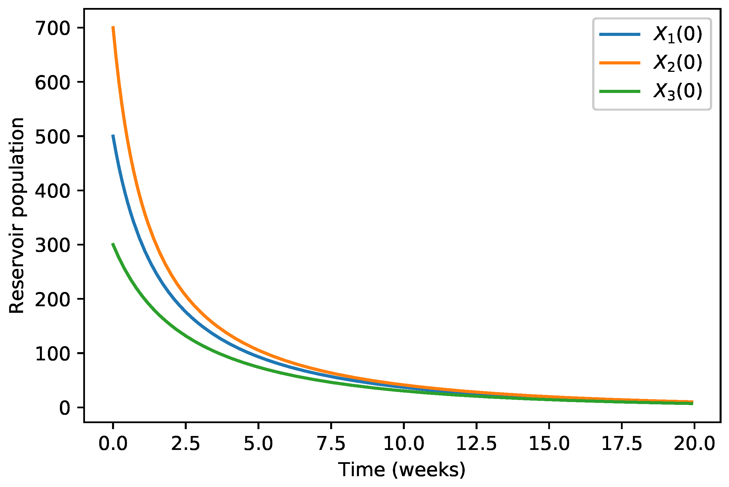
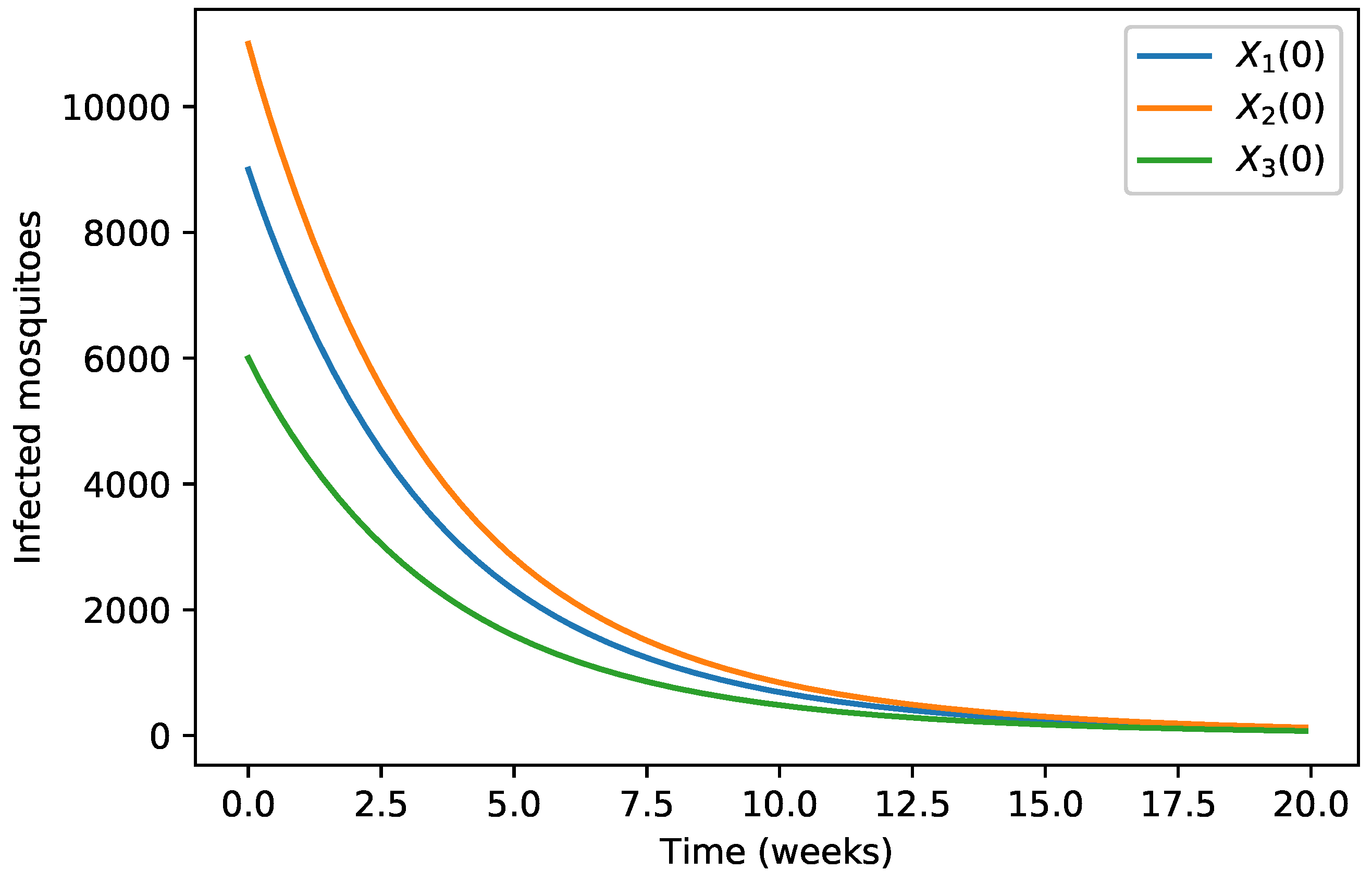
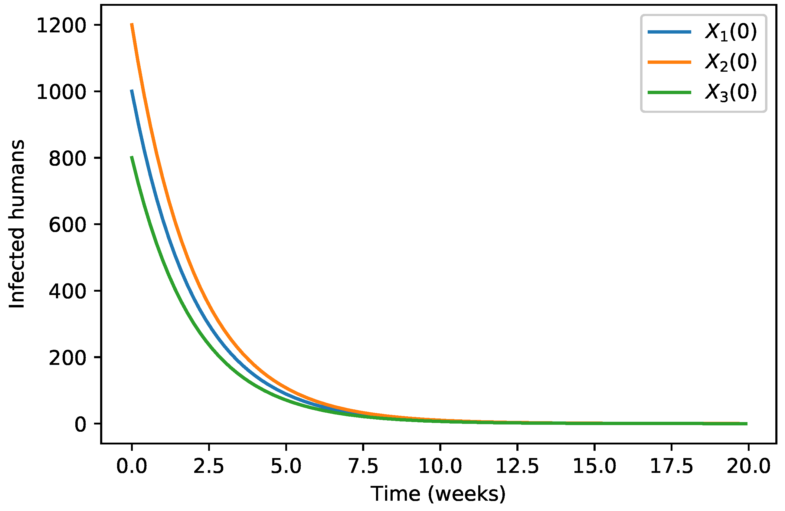
In this section, we illustrate stability and convergence of the solutions of the differential System (5) to the disease-free equilibrium (Equation (6)) for different values of initial conditions considered in

Table 1. Initial conditions considered.

	$\mathit{E}\left(0\right)$	${\mathit{I}}_{\mathit{r}}\left(0\right)$	${\mathit{A}}_{\mathit{m}}\left(0\right)$	${\mathit{N}}_{\mathit{m}}\left(0\right)$	${\mathit{I}}_{\mathit{m}}\left(0\right)$	$\mathit{N}\left(0\right)$	$\mathit{I}\left(0\right)$
$X_1\left(0\right)$	40,000	500	12,000	10,000	9000	7000	1000
$X_2\left(0\right)$	45,000	700	15,000	12,000	11,000	10,000	12,000
$X_3\left(0\right)$	35,000	300	10,000	7000	6000	5000	800

(see Figure 1, Figure 2 and Figure 3 for the corresponding infected populations in Model (5)). We perform numerical simulations to solve the model system (Model (5)) using the Python programming language, precisely the freely available routine integrate.odeint of library SciPy. The following values of the parameters, borrowed from [7,9], are considered:

$$\begin{array}{c}{Q}_0=50,\theta =0.0002,{\theta }_0=0.0001,{\beta }_{mr}=0.0001,{\mu }_{1r}=0.1,dr=1/15,\\ {\delta }_0=0.000001,{\mathsf{\Lambda }}_h=150,{\mu }_h=1/65,d_h=1/45,{\nu }_h=0.45,{\beta }_{mh}=0.0003,\\ \psi =0.6,K=1000,\delta =0.0001,{\mu }_m=0.3,{\beta }_{rm}=0.00021.\end{array}$$

Moreover, the remaining parameters were estimated as follows:

$$\begin{array}{c}{\mu }_{2r}=0.001,{\eta }_A=0.5,{\mu }_A=0.25,B=1.\end{array}$$

The value of the DFE, $E_2$ is computed as below:

$$E_2=\left(E^{*},I_r^{*},A_m^{*},N_m^{*},I_m^{*},N^{*},I^{*}\right)=\left(122.959,0,262.296,437.160,0,9750,0\right).$$

The matrices $J_{\mathcal{F}}$ and $J_{\mathcal{V}}$ are obtained as follows

$$J_{\mathcal{F}}=\left[\begin{array}{ccc}0.000123& 0& 0\\ 0.0918& 0& 0\\ 0& 0.0003& 0\end{array}\right],J_{\mathcal{V}}=\left[\begin{array}{ccc}0.167& 0& 0\\ 0& 0.3& 0\\ 0& 0& 0.488\end{array}\right],$$

which leads to the value of $R_0=0.000738$.

Furthermore, we have that the matrix M is equal to

$$M=\left[\begin{array}{ccccccc}-0.0001& 0& 0& 0& 0& 0& 0\\ 0& -0.167& 0& 0& 0& 0& 0\\ 0.0262& 0& -1& 0.443& 0& 0& 0\\ 0& 0& 0.5& -0.3& 0& 0& 0\\ 0& 0.0918& 0& 0& -0.3& 0& 0\\ 0& 0& 0& 0& 0& -0.0154& -0.0222\\ 0& 0& 0& 0& 0.0003& 0& -0.487\end{array}\right],$$

and its eigenvalues are

$$-1.236,-0.0636,-0.0001,-0.0154,-0.488,-0.3,-0.167$$

all negatives in accordance with Theorem 2, since $R_0<1$.

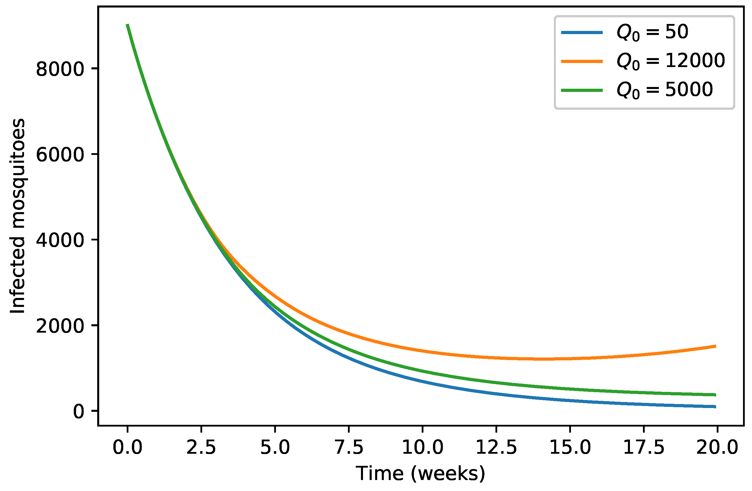
The initial conditions were considered as in Table 1 and the evolution of the three infected populations are strictly decreasing curves with all of them converging to the disease-free equilibrium (Figure 1, Figure 2 and Figure 3) for these specific parameter values.

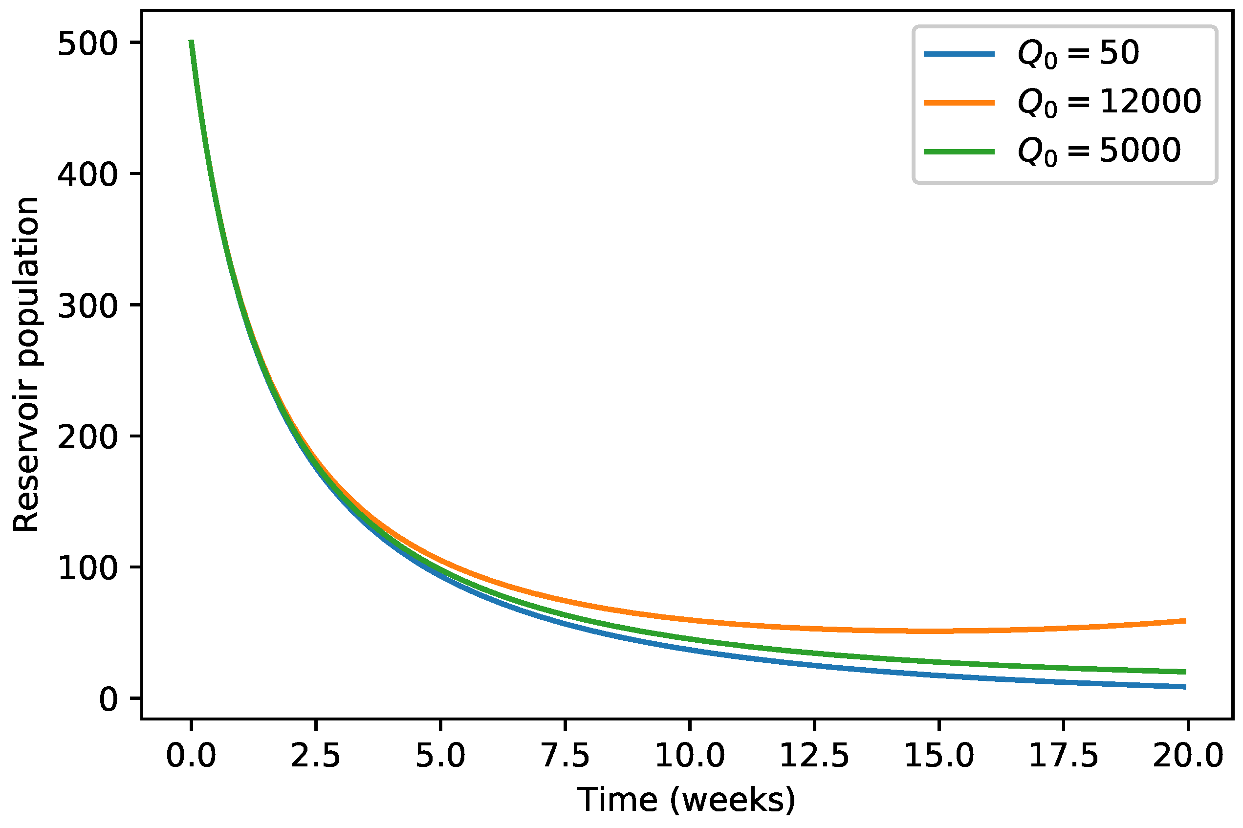
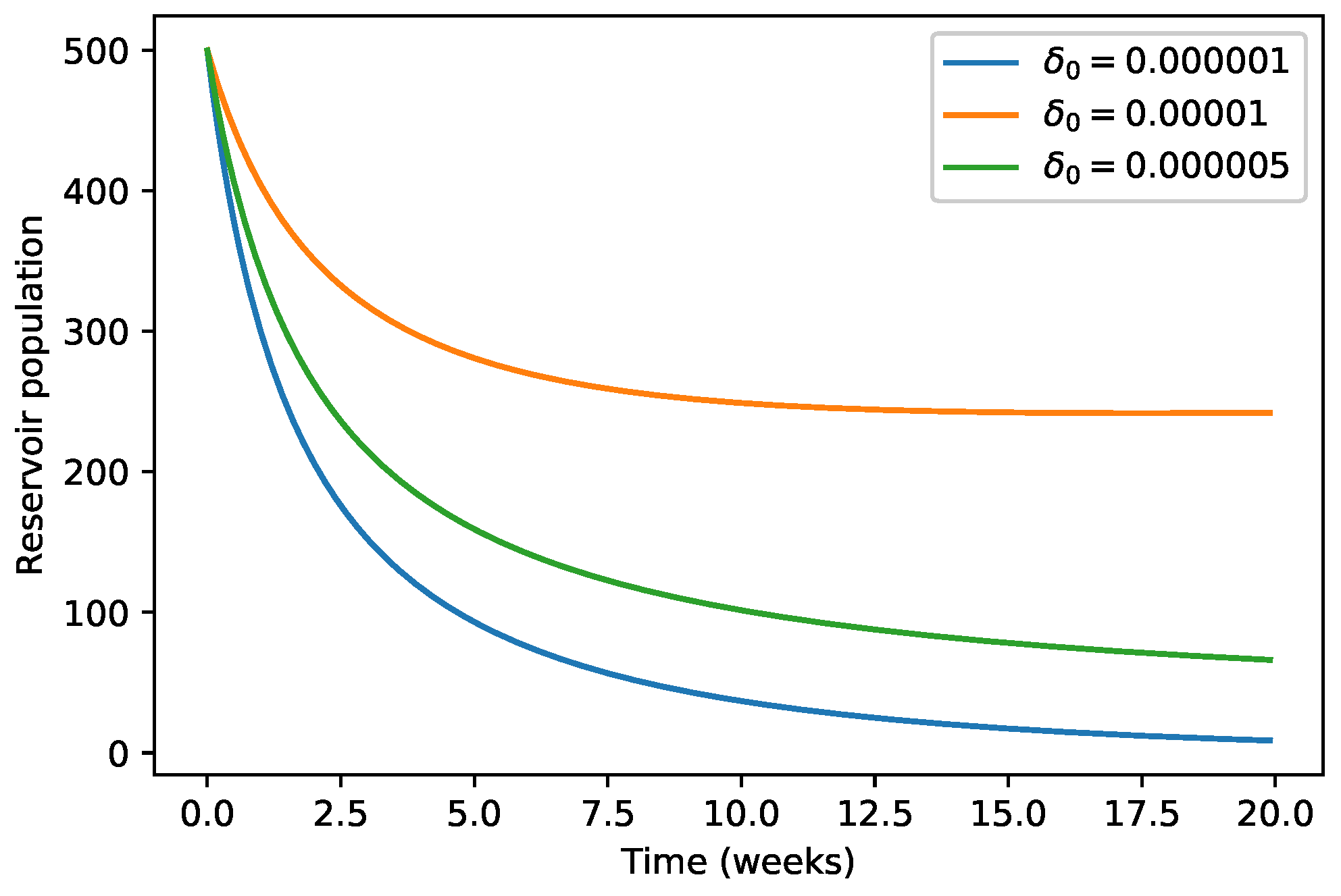
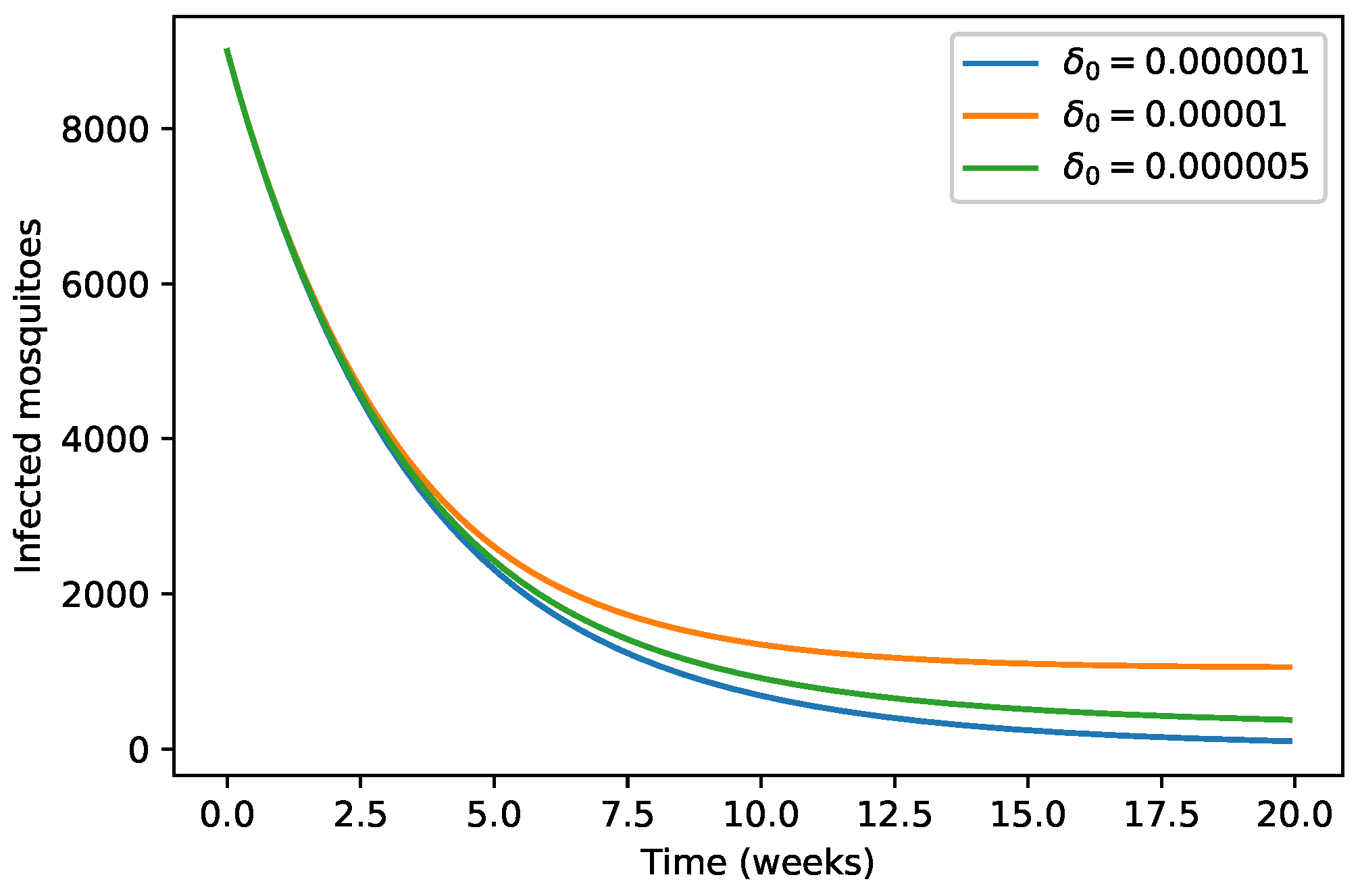
Our numerical simulations show that the evolution of the three infected populations are strictly decreasing curves, and all of them converge to the disease-free equilibrium (Figure 1, Figure 2 and Figure 3). This means that our Japanese Encephalitis model (Model (5)) describes a situation of an epidemic disease through an interesting environmental effect on the source of reproduction of mosquitoes, namely the aquatic phase of mosquitoes, which includes eggs, larva, and pupa stages. Furthermore, in  Figure 4 and Figure 5, the variation of the evolution of the infected animals population and infected mosquitoes population is shown, respectively, with respect to different values in the level of environmental discharge due to constant influx $\left(Q_0\right)$. It is found that with the decrease in the level of environmental discharge due to constant influx $\left(Q_0\right)$, the infected animals population and infected mosquitoes population decrease and approach the disease-free equilibrium state.

We observe in Figure 6 and Figure 7 that the decrease of the per capita growth rate ${\delta }_0$ of animals due to environmental discharges results in the decrease of the infected animals population as well as for the infected mosquitoes population.

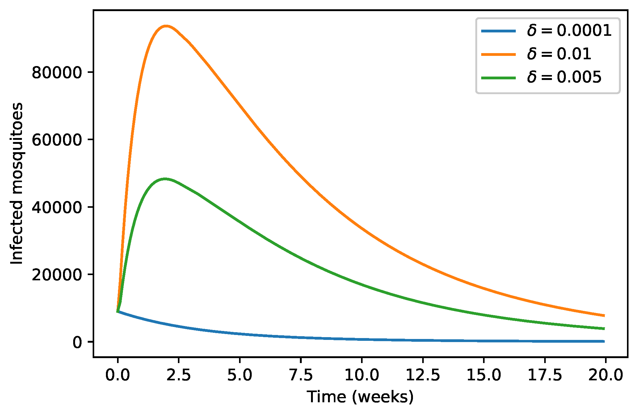
The role of conducive environmental discharge $\delta$ on the infected mosquitoes population is shown in Figure 8. We found that when the value of $\delta$ is smaller than $0.0001$, there is then a strict decrease in the number of infected mosquitoes population. However, when $\delta$ becomes larger, the infected mosquitoes population increases up to a certain optimum value and then decreases to the disease-free equilibrium state.

5. Conclusions

In [7], a Japanese Encephalitis model is studied. Its results show persistence of disease in the population—that is, an endemic situation. In contrast, our obtained results highlight the importance of considering environmental effects on the aquatic phase of mosquitoes as the primary source of reproduction of mosquitoes. This is not considered in [7], where the environmental effect is acting on the mature susceptible mosquitoes populations. Here, we have shown that the basic reproduction number is a linear dependent function with respect to the equilibrium state of the cumulative density of environmental discharges, conducive to the growth rate of mosquitoes and animals. All our computational experiments were carried out using the free and open-source scientific computing Python library SciPy. To make our results reproducible, we provide the main computer code in Appendix A. As future work, it would be interesting to validate the model with real data and take into account possible control measures, e.g., vaccination of the population and vector or environmental controls.

References

- Boyer, S.; Peng, B.; Pang, S.; Chevalier, V.; Duong, V.; Gorman, C.; Dussart, P.; Fontenille, D.; Cappelle, J. Dynamics and diversity of mosquito vectors of Japanese encephalitis virus in Kandal province, Cambodia. J. Asia-Pac. Entomol. 2020, 23, 1048–1054. [Google Scholar] [CrossRef]
- Wang, C.J.; Zeng, Z.L.; Zhang, F.S.; Guo, S.G. Clinical features of adult anti-N-methyl-d-aspartate receptor encephalitis after Japanese encephalitis. J. Neurol. Sci. 2020, 417, 117080. [Google Scholar] [CrossRef] [PubMed]
- Solomon, T.; Ni, H.; Beasley, D.; Ekkelenkamp, M.; Cardosa, M.; Barrett, A. Origin and evolution of Japanese encephalitis virus in southeast Asia. J. Virol. 2003, 77, 3091–3098. [Google Scholar] [CrossRef] [PubMed] [Green Version]
- Rodrigues, H.S.; Monteiro, M.T.T.; Torres, D.F.M. Seasonality effects on dengue: Basic reproduction number, sensitivity analysis and optimal control. Math. Methods Appl. Sci. 2016, 39, 4671–4679. [Google Scholar] [CrossRef] [Green Version]
- Ndaïrou, F.; Area, I.; Nieto, J.J.; Torres, D.F.M. Mathematical modeling of COVID-19 transmission dynamics with a case study of Wuhan. Chaos Solitons Fractals 2020, 135, 109846. [Google Scholar] [CrossRef] [PubMed]
- Lemos-Paião, A.P.; Silva, C.J.; Torres, D.F.M.; Venturino, E. Optimal control of aquatic diseases: A case study of Yemen’s cholera outbreak. J. Optim. Theory Appl. 2020, 185, 1008–1030. [Google Scholar] [CrossRef]
- Naresh, R.; Pandey, S. Modeling and analysis of the spread of Japanese encephalitis with environmental effects. Appl. Appl. Math. 2009, 4, 155–175. [Google Scholar]
- Agarwal, M.; Verma, V. The impact of media on the spreading and control of Japanese encephalitis. Int. J. Math. Sci. Comput. 2012, 2, 23–31. [Google Scholar]
- Panja, P.; Mondal, S.K.; Chattopadhyay, J. Stability and bifurcation analysis of Japanese encephalitis model with/without effects of some control parameters. Comput. Appl. Math. 2018, 37, 1330–1351. [Google Scholar] [CrossRef]
- Zhao, S.; Lou, Y.; Chiu, A.P.Y.; He, D. Modelling the skip-and-resurgence of Japanese encephalitis epidemics in Hong Kong. J. Theoret. Biol. 2018, 454, 1–10. [Google Scholar] [CrossRef] [PubMed]
- Ludwig, D. Final size distributions for epidemics. Math. Biosci. 1975, 23, 33–46. [Google Scholar] [CrossRef]
- Purdom, P.W. Environmental Health; Elsevier: New York, NY, USA, 2013. [Google Scholar]
- Ghosh, M.; Chandra, P.; Sinha, P.; Shukla, J.B. Modelling the spread of carrier-dependent infectious diseases with environmental effect. Appl. Math. Comput. 2004, 152, 385–402. [Google Scholar] [CrossRef]
- Ghosh, M.; Chandra, P.; Sinha, P.; Shukla, J.B. Modelling the spread of bacterial infectious disease with environmental effect in a logistically growing human population. Nonlinear Anal. Real World Appl. 2006, 7, 341–363. [Google Scholar] [CrossRef]
- Berge, T.; Bowong, S.; Lubuma, J.M.S. Global stability of a two-patch cholera model with fast and slow transmissions. Math. Comput. Simul. 2017, 133, 142–164. [Google Scholar] [CrossRef]
- Berge, T.; Lubuma, J.M.S.; Moremedi, G.M.; Morris, N.; Kondera-Shava, R. A simple mathematical model for Ebola in Africa. J. Biol. Dyn. 2017, 11, 42–74. [Google Scholar] [CrossRef] [PubMed] [Green Version]
- Codeço, C.T. Endemic and epidemic dynamic of cholera: The role of the aquatic reservoir. BMC Infect. Dis. 2001, 1, 14. [Google Scholar] [CrossRef] [PubMed] [Green Version]
- van den Driessche, P.; Watmough, J. Reproduction numbers and sub-threshold endemic equilibria for compartmental models of disease transmission. Math. Biosci. 2002, 180, 29–48. [Google Scholar] [CrossRef]
- Strogatz, S.H. Nonlinear Dynamics and Chaos: With Applications to Physics, Biology, Chemistry, and Engineering; Addison-Wesley Pub.: Reading, MA, USA, 1994. [Google Scholar]
Figure 1.
The solution of Model (5) tends toward the disease-free equilibrium. In this figure, we show the evolution of the infected animals population for different initial conditions.
Figure 2.
The solution of Model (5) tends toward the disease-free equilibrium. In this figure, we show the evolution of the infected mosquitoes population for different initial conditions.
Figure 3.
The solution of Model (5) tends toward the disease-free equilibrium. In this figure, we show the evolution of the infected humans population for different initial conditions.
Figure 4.
Variation of animals population with respect to .
Figure 5.
Variation of infected mosquitoes population with respect to .
Figure 6.
Figure 7.
Figure 8.