Packing Oblique 3D Objects

Abstract

Packing irregular 3D objects in a cuboid of minimum volume is considered. Each object is composed of a number of convex shapes, such as oblique and right circular cylinders, cones and truncated cones. New analytical tools are introduced to state placement constraints for oblique shapes. Using the phi-function technique, optimized packing is reduced to a nonlinear programming problem. Novel solution approach is provided and illustrated by numerical examples.

1. Introduction

Packing problems aim to allocate a set of objects in a container subject to placement constraints. The latter typically stipulates non-overlapping between the objects and the boundary of the container. Additional placement constraints may include weight distribution and stacking, cargo stability, balance constraints, loading and unloading preferences, etc. [1]. In optimized packing certain criteria have to be optimized, e.g., maximizing the number of the packed objects, minimizing the waste or optimizing characteristics of the container, its volume or shape [2]. Packing problems are proved to be NP-hard [3].

Packing issues traditionally are important in logistics, e.g., in maritime transportation and container loading, cutting industrial materials in furniture and glass manufacturing [4]. Packing problems also arise in modelling liquid and glass structures, in analyses of powder and granular materials in mineral industry, in molecular and nanotechnologies [5,6,7,8,9].

Different classifications for packing problems are proposed (see, e.g., [2,4,10] and the references therein). Focusing on the shapes involved, packing problems can be divided into two large groups: regular and irregular. While regular 3D packing deals with relatively simple shapes (spheres, ellipsoids, convex polyhedrons), irregular packing focuses basically on nonconvex figures (see, e.g., [2,11,12,13,14,15,16,17,18,19]).

Various modelling and solution approaches, exact and approximated, are known for the regular packing (see, e.g., [20,21,22] and the references therein). For irregular 3D packing, heuristics are widely used [2]. A large group of heuristics is based on representing complex irregular shapes by corresponding collections of simpler (regular) figures thus reducing the problem approximately to a regular case [23,24,25,26,27]. Techniques in the other group combine a local search with simple decision rules, such as the deepest bottom-left approach or random allocation [28,29,30,31,32,33]. An alternative methodology is using genetic algorithms, directly or in combination with the first two approaches [34,35,36,37].

In this paper, packing irregular 3D objects in a cuboid of minimum volume is considered. Each complex object is composed of a number of convex shapes, such as oblique and right circular cylinders, cones and truncated cones. Studying composed objects requires new modelling tools, different from those used previously for simpler objects (see, e.g., [20,21,22] and the references therein). In this paper, the phi-function approach is applied to represent analytically containment and non-overlapping conditions. Using the concept of quasi phi-functions [38], an exact mathematical model is formulated and a corresponding nonlinear programming problem is stated. A solution algorithm is proposed and computational results are presented to illustrate the approach. To the best of our knowledge, exact mathematical models for packing complex objects composed of a mixture of oblique and right convex shapes nether were considered before.

Nonspherical particles presented by the superquadric equations are widely used in different industrial production, and significantly affect the macro- and microcharacteristics of granular materials, see, e.g., [39] and the references therein. However, the particle shapes constructed by the superquadric equations are geometrically symmetrical and strictly convex, which significantly limits their further engineering applications [40]. In recent years, the composed element method has been successfully used. In this approach a complex nonconvex object is composed of basic convex elements, e.g., spheres, cylinders, super-quadratic elements and other convex (irregular) shapes [41,42].

Another source of packing complex composed shapes is additive manufacturing (AM), also known as 3D printing. AM refers to technologies for producing complex parts in a layer-by-layer material deposition process. The process takes place inside the machine in an enclosed build container or a “build volume”. AM does not use any conventional physical tooling such as moulds, cutting implements or dies. Using AM, products previously designed and manufactured as assemblies of multiple components can now be manufactured as single items [43]. As a parallel manufacturing process, AM permits producing various complex parts in a single build volume. This gives rise to a build volume packing problem arising during the machine setup process. Thus, packing complex objects composed of different shapes plays an important role 3D printing.

Our interest in studying oblique objects is motivated by modelling particulate systems of nonspherical shapes [44,45] and by build volume packing problems in 3D printing [10].

The main contributions of the paper are as follows:

• New tools of mathematical modelling are presented to describe analytically non-overlapping and containment constraints for packing irregular 3D objects composed by the union of oblique and right basic shapes (circular cylinders, cones, truncated cones and spheres). The objects can be freely translated and rotated.
• An exact mathematical model for the irregular packing problem is formulated in the form of nonlinear continuous programming problem.
• A solution algorithm for the irregular packing problem is developed.
• New benchmark instances are provided to illustrate the efficiency of the approach.

The paper is organized as follows. Section 2 provides the general formulation for the irregular packing problem. Quasi-phi-function s for the composed 3D objects are defined to describe analytically placement constraints in Section 3. The nonlinear programming model for the irregular packing problem is presented and solved by an algorithm described in Section 4. Computational results are given in Section 5, while Section 6 concludes. Definitions of the phi-functions and quasi-phi-function s are provided in Appendix A.

2. Problem Formulation

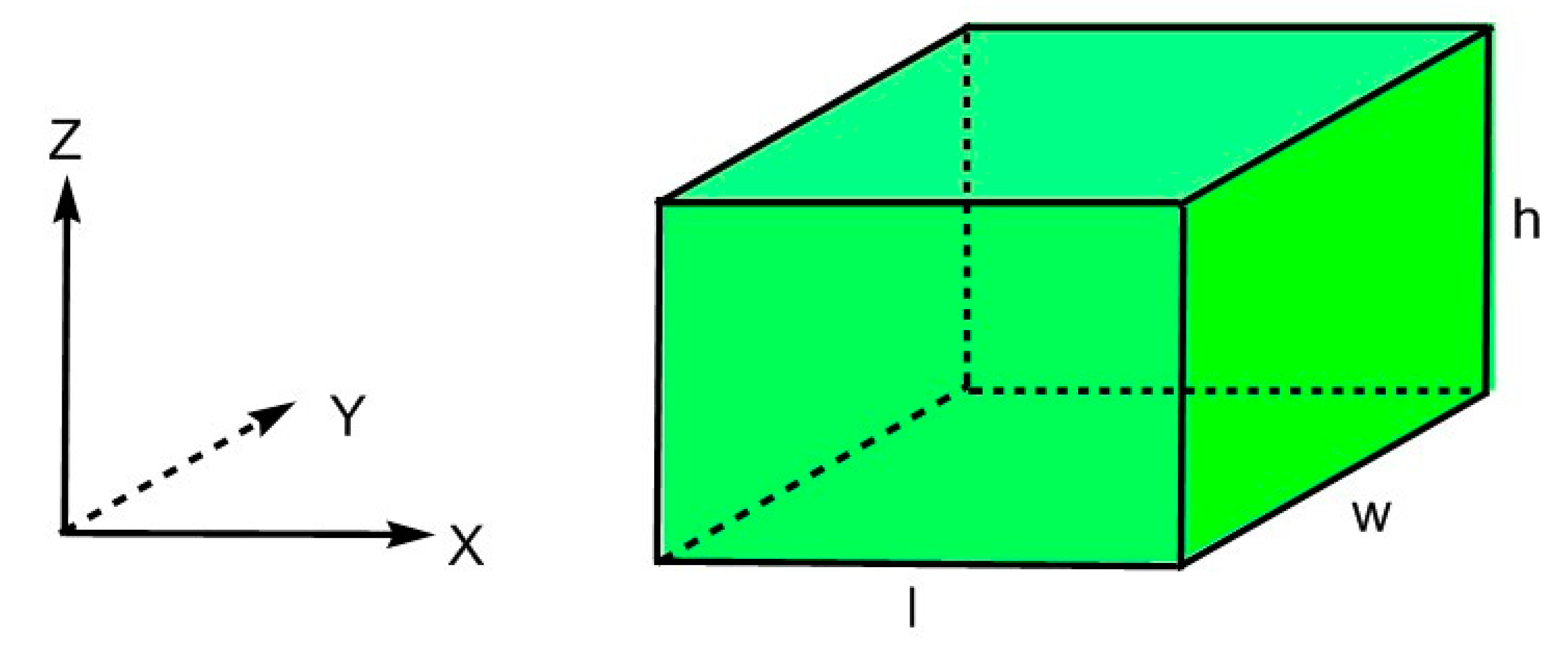
The packing problem is considered in the following setting. Denote a cuboid of variable length $l$, width $w$ and height $h$ by $\Omega$ (see Figure 1). Let a set of objects $T_q\subset {\mathbb{R}}^3,$ $q\in J_N=$ $\{1,2,\dots ,N\}$ be given.

The location and orientation of each 3D object $T_q$ is defined by a vector $u_q=(v_q,{\mathsf{\theta }}_q)$ of its (variable) placement parameters in the fixed coordinate system $OXYZ$. Here $v_q=(x_q,y_q,z_q)$ is a translation vector and ${\mathsf{\theta }}_q=({\mathsf{\theta }}_q^1,{\mathsf{\theta }}_q^2,{\mathsf{\theta }}_q^3)$ is a vector of rotation parameters, where ${\mathsf{\theta }}_q^1,{\mathsf{\theta }}_q^2,{\mathsf{\theta }}_q^3$ are Euler angles.

The notation $T_q(u_q)=\{\tilde{p}\in {\mathbb{R}}^3:\tilde{p}=v_q+\Theta ({\mathsf{\theta }}_q)\cdot {(p)}^T,\forall p\in T_q\}$ is used for translated and rotated object $T_q^{}$, where $\Theta ({\mathsf{\theta }}_q)=\Theta ({\mathsf{\theta }}_q^1,{\mathsf{\theta }}_q^2,{\mathsf{\theta }}_q^3)$ is a rotation matrix of the form:

$$\begin{array}{l}\Theta ({\mathsf{\theta }}_q)=\left(\begin{array}{ccc}\cos {\mathsf{\theta }}_q^1\cos {\mathsf{\theta }}_q^3-\sin {\mathsf{\theta }}_q^1\cos {\mathsf{\theta }}_q^2\sin {\mathsf{\theta }}_q^3& -\cos {\mathsf{\theta }}_q^1\sin {\mathsf{\theta }}_q^3-\sin {\mathsf{\theta }}_q^1\cos {\mathsf{\theta }}_q^2\cos {\mathsf{\theta }}_q^3& \sin {\mathsf{\theta }}_q^1\sin {\mathsf{\theta }}_q^2\\ \sin {\mathsf{\theta }}_q^1\cos {\mathsf{\theta }}_q^3+\cos {\mathsf{\theta }}_q^1\cos {\mathsf{\theta }}_q^2\sin {\mathsf{\theta }}_q^3& -\sin {\mathsf{\theta }}_q^1\sin {\mathsf{\theta }}_q^3+\cos {\mathsf{\theta }}_q^1\cos {\mathsf{\theta }}_q^2\cos {\mathsf{\theta }}_q^3& -\cos {\mathsf{\theta }}_q^1\sin {\mathsf{\theta }}_q^2\\ \sin {\mathsf{\theta }}_q^2\sin {\mathsf{\theta }}_q^3& \sin {\mathsf{\theta }}_q^2\cos {\mathsf{\theta }}_q^3& \cos {\mathsf{\theta }}_q^2\end{array}\right).\\ \end{array}$$

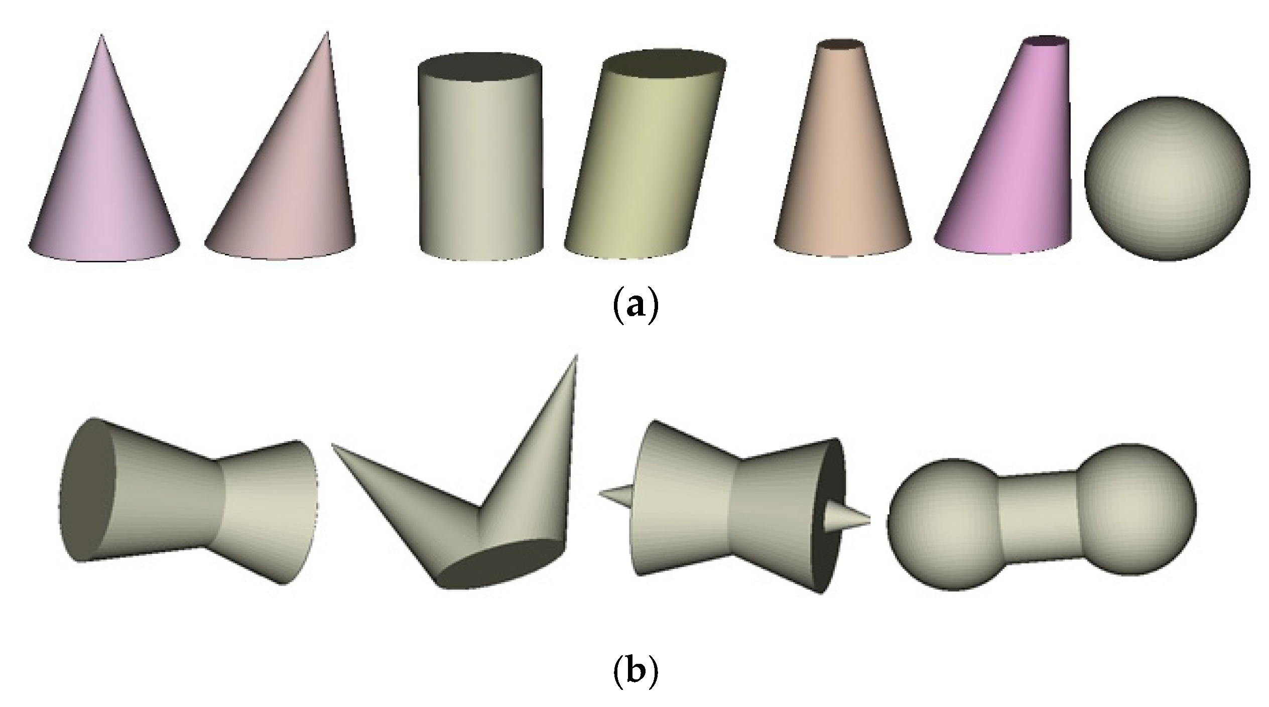
Assume that $T_q(u_q)={\displaystyle \underset{i=1}{\overset{n_q}{{\displaystyle \cup }}}{T}_i^q}(u_q)$, where $T_i^q$ denotes a basic object from a family of oblique and right circular cylinders, cones, truncated cones denoted by $\Im$ and spheres (Figure 2a). An object $T_q$ for $n_q\ge 2$ is referred to the composed object (Figure 2b).

Let a sphere be defined by its centre $p_i^q=(x_i^q,y_i^q,z_i^q)$ and a radius $r_i^q$. Each basic object from the family $\Im$ is defined by three vectors $p_{i1}^q=(x_{i1}^q,y_{i1}^q,z_{i1}^q)$, $p_{i2}^q=(x_{i2}^q,y_{i2}^q,z_{i2}^q)$ and $n_i^q=({\mathrm{n}}_i^x,{\mathrm{n}}_i^y,{\mathrm{n}}_i^z)$, as well as a pair of parameters $r_{i1}^q$ and $r_{i2}^q$. Here $p_{i1}^q$, $p_{i2}^q$ are the centres and $r_{i1}^q$, $r_{i2}^q$ are the radii of the bottom and top bases of $T_i^q$, $n_i^q$ is the unit normal vector to the bottom (top) base of $T_i^q$.

Note that if $r_{i1}^q=r_{i2}^q>0$ then $T_i^q$ is a circular cylinder; if $r_{i1}^q\ne r_{i2}^q$ and $r_{i1}^q>0,r_{i2}^q>0$ then $T_i^q$ is a circular truncated cone; if $r_{i1}^q>0,r_{i2}^q=0$ or $r_{i1}^q=0,r_{i2}^q>0$ then $T_i^q$ is a circular cone. The height of each object $T_i^q\in \Im$ is denoted by $h_i^q$.

Let $p_i^q=(x_i^q,y_i^q,z_i^q)$ be a reference point of the basic object $T_i^q\subset$ $T_q$: the centre point of a sphere or the central point for a circular base of the objects from the family $\Im$. In what follows, notation ${\tilde{p}}_i^q=({\tilde{x}}_i^q,{\tilde{y}}_i^q,{\tilde{z}}_i^q)=v_q+\Theta ({\mathsf{\theta }}_q)\cdot {(p_i^q)}^T$ is used, where $v_q$ is the translation vector and $\Theta ({\mathsf{\theta }}_q)$ is the rotation matrix of the object $T_q^{}$.

The placement constraints can be stated in the following form:

$$\mathrm{int}{T}_q(u_q)\cap \mathrm{int}{T}_g(u_g)=Ø\mathrm{for}q>g\in J_N,$$

(1)

$$T_q(u_q)\subset \Omega \mathrm{for}q\in J_N.$$

(2)

Conditions (1) describe non-overlapping for all pairs of objects $T_q(u_q)$ and $T_g(u_g)$ for $q>g\in J_N$ (further, non-overlapping constraints), while conditions (2) assure containing $T_q(u_q)$ in the container $\Omega$ for $q\in J_N$ (further, containment constraints).

Irregularpacking problem. Pack the set of objects $T_q$, $q\in J_N$, within a cuboidal container $\Omega$ of minimal volume $\mathsf{\kappa }=l\cdot w\cdot h$, taking into account the placement constraints (1)–(2).

3. Analytical Tools

In this section geometric tools for the mathematical modelling of the placement constraints (1) and (2) are presented. To describe analytically the relations between a pair of objects considered in the placement constraints, the phi-functions [38] and quasi-phi-functions [18] are used (see Appendix A for the details. These functions for irregular objects composed of oblique and right shapes are introduced in this paper for the first time.

3.1. Modeling Non-Overlapping Constraints

Consider a pair of the composed objects $T_q(u_q)={\displaystyle \underset{i=1}{\overset{n_q}{{\displaystyle {\displaystyle \cup }}}}{T}_i^q(u_q)}$ and $T_g(u_g)={\displaystyle \underset{j=1}{\overset{n_g}{{\displaystyle \cup }}}{T}_j^g}(u_g)$.

To describe non-overlapping constraints (1) a phi-function for two composed objects $T_q(u_q)$ and $T_g(u_g)$ is introduced. It can be written in the form

$${{\mathsf{\Phi }}^{\prime }}_{qg}^{}(u_q,u_g,{\mathsf{\tau }}_{qg}^{})=\underset{i=1,..,n_q,j=1,\dots ,n_g}{\min }{{\mathsf{\Phi }}^{\prime }}_{ij}^{qg}(u_q,u_g,{\mathsf{\tau }}_{ij}^{qg})$$

(3)

where ${\mathsf{\tau }}_{qg}^{}=({\mathsf{\tau }}_{ij}^{qg},i=1,\dots ,n_q,j=1,\dots ,n_q)$, ${{\mathsf{\Phi }}^{\prime }}_{ij}^{qg}(u_q,u_g,{\mathsf{\tau }}_{ij}^{qg})$ is an adjusted quasi-phi-function for convex objects $T_i^q(u_q)$ and $T_j^g(u_g)$.

Let $P_{ij}^{qg}=\{(x,y,z):x\le 0\}$ be a half space. Denote the half-space $P$ translated along OX on value ${\mathsf{\mu }}_{ij}^{qg}$ and rotated by angles ${\mathsf{\theta }}^1$, ${\mathsf{\theta }}^2$, by ${\tilde{P}}_{ij}^{qg}=\{p:{\mathsf{\Psi }}_{ij}^{qg}(p,{\mathsf{\tau }}_{ij}^{qg})\le 0\}$, where

$${\mathsf{\Psi }}_{ij}^{qg}(p,{\mathsf{\tau }}_{ij}^{qg})=\cos {\mathsf{\theta }}_{ij}^{1qg}\cdot \cos {\mathsf{\theta }}_{ij}^{2qg}\cdot x-\sin {\mathsf{\theta }}_{ij}^{2qg}\cdot y+\sin {\mathsf{\theta }}_{ij}^{1qg}\cdot \cos {\mathsf{\theta }}_{ij}^{2qg}\cdot z+{\mathsf{\mu }}_{ij}^{qg}$$

(4)

$p=(x,y,z)$, ${\mathsf{\tau }}_{ij}^{qg}=({\mathsf{\theta }}_{ij}^{1qg},{\mathsf{\theta }}_{ij}^{2qg},{\mathsf{\mu }}_{ij}^{qg})$, ${\mathsf{\theta }}_{ij}^{1qg}$ and ${\mathsf{\theta }}_{ij}^{2qg}$ are rotation angles of the half space $P_{ij}^{qg}$ around the axes OY and OZ in the fixed coordinate system. Define the plane ${\tilde{L}}_{ij}^{qg}=\{(x,y,z):{\mathsf{\Psi }}_{ij}^{qg}(p,\mathsf{\tau })=0\}$.

A quasi-phi-function for convex basic objects$T_i^q(u_q)$and$T_j^g(u_g)$ can be defined in the form

$${{\mathsf{\Phi }}^{\prime }}_{ij}^{qg}(u_q,u_g,{\mathsf{\tau }}_{ij}^{qg})=\min \{{\mathsf{\Phi }}_i^q(u_q,{\mathsf{\tau }}_{ij}^{qg}),{\mathsf{\Phi }}_j^{*g}(u_g,{\mathsf{\tau }}_{ij}^{qg})\}$$

(5)

where ${\mathsf{\Phi }}_i^q(u_q,{\mathsf{\tau }}_{ij}^{qg})$ is a phi-function for the object $T_i^q(u_q)$ and the half space ${\tilde{P}}_{ij}^{qg}$, ${\mathsf{\Phi }}_j^{*g}(u_g,{\mathsf{\tau }}_{ij}^{qg})$ is a phi-function for the object $T_j^g(u_g)$ and the half space ${\tilde{P}}^{*}{}_{ij}^{qg}={\mathbb{R}}^3\backslash \mathrm{int}{\tilde{P}}_{ij}^{qg}$. Here ${\mathsf{\tau }}_{ij}^{qg}=({\mathsf{\theta }}_{ij}^{1qg},{\mathsf{\theta }}_{ij}^{2qg},{\mathsf{\mu }}_{ij}^{qg})$ is the vector of auxiliary variables of the quasi-phi-function ${{\mathsf{\Phi }}^{\prime }}_{ij}^{qg}$.

Therefore to define the quasi-phi-functions (5) for each pair of convex basic objects the phi-functions ${\mathsf{\Phi }}_i^q(u_q,{\mathsf{\tau }}_{ij}^{qg})$ and ${\mathsf{\Phi }}_j^{*g}(u_g,{\mathsf{\tau }}_{ij}^{qg})$ have to be derived.

First, define the phi-function ${\mathsf{\Phi }}_i^q(u_q,{\mathsf{\tau }}_{ij}^{qg})$ for the basic object $T_i^q(u_q)$ and the half space ${\tilde{P}}_{ij}^{qg}$.

Let $T_i^q(u_q)$ be a sphere centred at the point ${\tilde{p}}_{i1}^q=({\tilde{x}}_i^q,{\tilde{y}}_i^q,{\tilde{z}}_i^q)$ and having its radius $r_i^q$.

The phi-function for the sphere $T_i^q(u_q)$ and a half space ${\tilde{P}}_{ij}^{qg}$ has the form

$$\begin{gathered} {\mathsf{\Phi }}_i^q(u_q,{\mathsf{\tau }}_{ij}^{qg})=\cos {\mathsf{\theta }}_{ij}^{1qg}\cdot \cos {\mathsf{\theta }}_{ij}^{2qg}\cdot {\tilde{x}}_{i1}^q-\sin {\mathsf{\theta }}_{ij}^{2qg}\cdot {\tilde{y}}_{i1}^q+\sin {\mathsf{\theta }}_{ij}^{1qg}\cdot \cos {\mathsf{\theta }}_{ij}^{2qg}\cdot {\tilde{z}}_{i1}^q+{\mathsf{\mu }}_{ij}^{qg}-r_i^q= \\ {\tilde{n}}_{ij}^{qg}\cdot {\tilde{p}}_{i1}^q+{\mathsf{\mu }}_{ij}^{qg}-r_i^q, \end{gathered}$$

while the phi-function for the sphere $T_j^g(u_g)$ and the half space ${\tilde{P}}^{*}{}_{ij}^{qg}$ can be defined as follows

$$\begin{gathered} {\mathsf{\Phi }}_j^{*g}(u_g,{\mathsf{\tau }}_{ij}^{qg})=-\cos {\mathsf{\theta }}_{ij}^{1qg}\cdot \cos {\mathsf{\theta }}_{ij}^{2qg}\cdot {\tilde{x}}_{i1}^q+\sin {\mathsf{\theta }}_{ij}^{2qg}\cdot {\tilde{y}}_{i1}^q-\sin {\mathsf{\theta }}_{ij}^{1qg}\cdot \cos {\mathsf{\theta }}_{ij}^{2qg}\cdot {\tilde{z}}_{i1}^q-{\mathsf{\mu }}_{ij}^{qg}-r_i^q= \\ -{\tilde{n}}_{ij}^{qg}\cdot {\tilde{p}}_{i1}^q-{\mathsf{\mu }}_{ij}^{qg}-r_i^q. \end{gathered}$$

For $T_i^q(u_q)$ from the family $\Im$, let the bottom base of $T_i^q(u_q)$ is a circle centred at the point ${\tilde{p}}_{i1}^q=({\tilde{x}}_i^q,{\tilde{y}}_i^q,{\tilde{z}}_i^q)$ and having its radius $r_{i1}^q$, while the top circular base of $T_i^q(u_q)$ is centred at ${\tilde{p}}_{i2}^q=({\tilde{x}}_i^q,{\tilde{y}}_i^q,{\tilde{z}}_i^q+h_i^q)$ and has its radius $r_{i2}^q$ (the cone corresponds to $r_{i2}^q=0$).

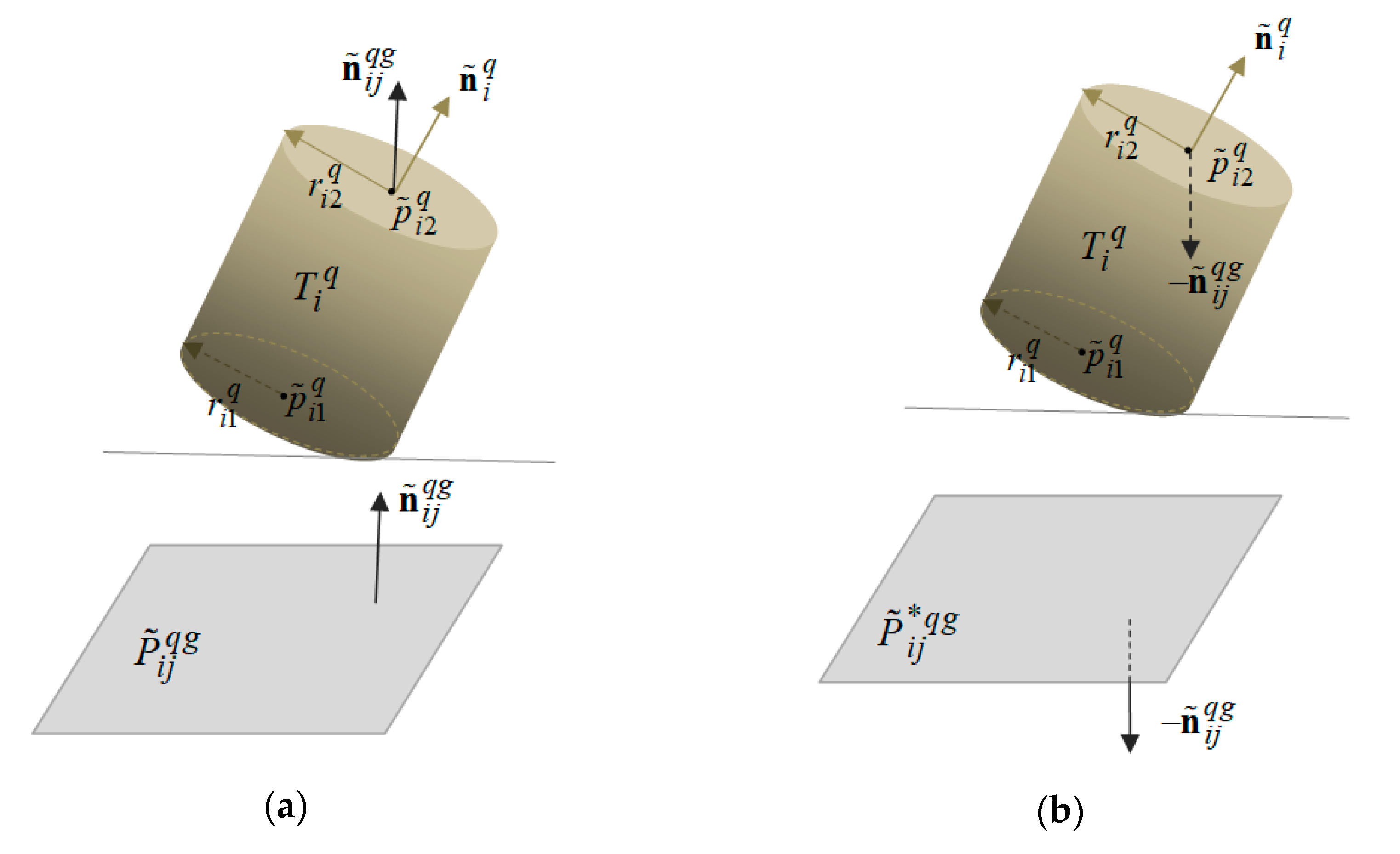
The phi-function for the object $T_i^q(u_q)\in \Im$ and a half space ${\tilde{P}}_{ij}^{qg}$ has the form

$${\mathsf{\Phi }}_i^q(u_q,{\mathsf{\tau }}_{ij}^{qg})=\min \{f_1(u_q,{\mathsf{\tau }}_{ij}^{qg}),f_2(u_q,{\mathsf{\tau }}_{ij}^{qg})\},$$

$$f_1(u_q,{\mathsf{\tau }}_{ij}^{qg})={\tilde{n}}_{ij}^{qg}\cdot {\tilde{p}}_{i1}^q+{\mathsf{\mu }}_{ij}^{qg}-r_{i1}^q\sqrt{1-{({\tilde{n}}_{ij}^{qg}\cdot {\tilde{n}}_i^q)}^2},$$

$$f_2(u_q,{\mathsf{\tau }}_{ij}^{qg})={\tilde{n}}_{ij}^{qg}\cdot {\tilde{p}}_{i2}^q+{\mathsf{\mu }}_{ij}^{qg}-r_{i2}^q\sqrt{1-{({\tilde{n}}_{ij}^{qg}\cdot {\tilde{n}}_i^q)}^2},$$

where ${\tilde{n}}_{ij}^{qg}=({\tilde{n}}_{ij}^x,{\tilde{n}}_{ij}^y,{\tilde{n}}_{ij}^z)$ denotes a unit vector of the external normal to the half space ${\tilde{P}}_{ij}^{qg}$ and ${\tilde{n}}_i^q=({\tilde{n}}_i^x,{\tilde{n}}_i^y,{\tilde{n}}_i^z)$ stands for a unit vector of the external normal to the object $T_i^q(u_q)$ (see Figure 3).

The phi-function for the object $T_j^g(u_g)$ and a half space ${\tilde{P}}^{*}{}_{ij}^{qg}$ has the form

$${\mathsf{\Phi }}_j^{*g}(u_g,{\mathsf{\tau }}_{ij}^{qg})=\min \{f_1(u_g,{\mathsf{\tau }}_{ij}^{qg}),f_2(u_g,{\mathsf{\tau }}_{ij}^{qg})\},$$

$$f_1(u_g,{\mathsf{\tau }}_{ij}^{qg})=-{\tilde{n}}_{ij}^{qg}\cdot {\tilde{p}}_{j1}^g-{\mathsf{\mu }}_{ij}^{qg}-r_{j1}^g\sqrt{1-{({\tilde{n}}_{ij}^{qg}\cdot {\tilde{n}}_i^q)}^2},$$

$$f_2(u_g,{\mathsf{\tau }}_{ij}^{qg})=-{\tilde{n}}_{ij}^{qg}\cdot {\tilde{p}}_{j2}^g-{\mathsf{\mu }}_{ij}^{qg}-r_{j2}^g\sqrt{1-{({\tilde{n}}_{ij}^{qg}\cdot {\tilde{n}}_i^q)}^2}.$$

The inequality ${{\mathsf{\Phi }}^{\prime }}_{qg}^{}(u_q,u_g,{\mathsf{\tau }}_{qg}^{})\ge 0$ assures the non-overlapping condition $\mathrm{int}{T}_q(u_q)\cap \mathrm{int}{T}_g(u_g)=Ø$ in (1).

3.2. Modeling the Containment Constraints

Let us express the containment constraint $T_q(u_q)\subset \Omega$ in the equivalent form as $\mathrm{int}{T}_q(u_q)\cap {\Omega }^{*}=Ø$, where ${\Omega }^{*}=R^3\backslash \mathrm{int}\Omega$.

The phi-function for the objects $T_q(u_q)={\displaystyle \underset{i=1}{\overset{n_q}{{\displaystyle \cup }}}{T}_i^q(u_q)}$ and ${\Omega }^{*}$ can be defined in the form:

$${\mathsf{\Phi }}_q(u_q)=\underset{i=1,..,n_q}{\min }{\mathsf{\Phi }}_i^q(u_q),$$

(6)

where ${\mathsf{\Phi }}_i^q(u_q)$ is the phi-function for the basic convex object $T_i^q(u_q)$ and the object ${\Omega }^{*}$.

The inequality ${\mathsf{\Phi }}_q(u_q)\ge 0$ implies fulfilling the condition $\mathrm{int}{T}_q(u_q)\cap {\Omega }^{*}=Ø$ that describes the containment condition (2).

Containment of a sphere$T_i^q(u_q)$in a cuboid$\Omega$. The phi-function for the sphere $T_i^q(u_q)$ and the object ${\Omega }^{*}$ can be defined by the equation

$${\mathsf{\Phi }}_i^q(u_q)=\min \{l-{\tilde{p}}_{i1}^{qx}-r_{i1}^q,w-{\tilde{p}}_{i1}^{qy}-r_{i1}^q,h-{\tilde{p}}_{i1}^{qz}-r_{i1}^q,{\tilde{p}}_{i1}^{qx}-r_{i1}^q,{\tilde{p}}_{i1}^{qy}-r_{i1}^q,{\tilde{p}}_{i1}^{qz}-r_{i1}^q\}.$$

Containment of the object$T_i^q(u_q)$from the family$\Im$in a cuboid$\Omega$. The phi-function for the objects $T_i^q(u_q)$ and ${\Omega }^{*}$ has the form

$${\mathsf{\Phi }}_i^q(u_q)=\min \{{\mathsf{\phi }}_k(u_q),k=1,\dots ,6\}$$

(7)

where

$${\mathsf{\phi }}_1(u_q)=\min \{{\tilde{p}}_{i1}^{qx}-r_{i1}^q\sqrt{1-{({\tilde{\mathrm{n}}}_i^{qx})}^2},{\tilde{p}}_{i2}^{qx}-r_{i2}^q\sqrt{1-{({\tilde{\mathrm{n}}}_i^{qx})}^2}\},$$

$${\mathsf{\phi }}_2(u_q)=\min \{{\tilde{p}}_{i1}^{qy}-r_{i1}^q\sqrt{1-{({\tilde{\mathrm{n}}}_i^{qy})}^2},{\tilde{p}}_{i2}^{qy}-r_{i2}^q\sqrt{1-{({\tilde{\mathrm{n}}}_i^{qy})}^2}\},$$

$${\mathsf{\phi }}_3(u_q)=\min \{{\tilde{p}}_{i1}^{qz}-r_{i1}^q\sqrt{1-{({\tilde{\mathrm{n}}}_i^{qz})}^2},{\tilde{p}}_{i2}^{qz}-r_{i2}^q\sqrt{1-{({\tilde{\mathrm{n}}}_i^{qz})}^2}\},$$

$${\mathsf{\phi }}_4(u_q)=\min \{l-{\tilde{p}}_{i1}^{qx}-r_{i1}^q\sqrt{1-{({\tilde{\mathrm{n}}}_i^{qx})}^2},l-{\tilde{p}}_{i2}^{qx}-r_{i2}^q\sqrt{1-{({\tilde{\mathrm{n}}}_i^{qx})}^2}\},$$

$${\mathsf{\phi }}_5(u_q)=\min \{w-{\tilde{p}}_{i1}^{qy}-r_{i1}^q\sqrt{1-{({\tilde{\mathrm{n}}}_i^{qy})}^2},w-{\tilde{p}}_{i2}^{qy}-r_{i2}^q\sqrt{1-{({\tilde{\mathrm{n}}}_i^{qy})}^2}\},$$

$${\mathsf{\phi }}_6(u_q)=\min \{h-{\tilde{p}}_{i1}^{qz}-r_{i1}^q\sqrt{1-{({\tilde{\mathrm{n}}}_i^{qz})}^2},h-{\tilde{p}}_{i2}^{qz}-r_{i2}^q\sqrt{1-{({\tilde{\mathrm{n}}}_i^{qz})}^2}\}.$$

The inequality ${\mathsf{\Phi }}_i^q(u_q)\ge 0$ implies the condition $\mathrm{int}{T}_i^q(u_q)\cap {\Omega }^{*}=Ø$.

4. Mathematical Model and Solution Algorithm

4.1. Mathematical Model

Now the irregular packing problem can be formulated as the following nonlinear optimization problem:

$$\min \mathsf{\kappa }\mathrm{s}.\mathrm{t}.\left(u,\mathsf{\tau }\right)\in W,$$

(8)

$$W=\{(u,\mathsf{\tau }):{{\mathsf{\Phi }}^{\prime }}_{qg}(u_q,u_g,{\mathsf{\tau }}_{qg})\ge 0,q>g\in I_N,{\mathsf{\Phi }}_q(u_q)\ge 0,q\in I_N\},$$

(9)

where ${\mathsf{\tau }}_{qg}^{}=({\mathsf{\tau }}_{ij}^{qg},i=1,\dots ,n_q,j=1,\dots ,n_q)$ is a vector of the auxiliary variables for the quasi-phi-function ${{\mathsf{\Phi }}^{\prime }}_{qg}(u_q,u_g,{\mathsf{\tau }}_{qg})$ (3)–(5) for the objects $T_q(u_q)$ and $T_g(u_g)$, ${\mathsf{\Phi }}_q(u_q)$ is the phi-function (6)–(7) for the objects $T_q(u_q)$ and ${\Omega }^{*}$, $q\in I_N$.

The feasible region $W$ in (9) is defined by a system of nonsmooth inequalities that can be reduced to a system of inequalities with differentiable functions.

The model (8)–(9) is a nonconvex and continuous nonlinear programming problem. This is an exact formulation in the sense that it gives all optimal solutions to the irregular packing problem.

The number of the problem variables is $\sigma =3(1+2N+m)$, where $m={\displaystyle \sum _{q>g\in I_N}{n}_q{n}_g}$. The model (8)–(9) involves $O(N^2)$ nonlinear inequalities and $O(N^2)$ variables.

The model (8)–(9) represents all globally optimal solutions to the original irregular packing problem. It can be solved by any available global solver, e.g., BARON or LGO included in AMPL [46]. However, due to large number of variables and constraints, a direct solution to this problem may be time consuming and complicated. In the next section a solution approach is proposed to search for a local minimum of the problem (8)–(9). This solution can be used either as a reasonable approximation to the original global solution, or as a starting point for a global solver or heuristics.

4.2. Solution Algorithm

The following multistart strategy is used to solve the problem (8)–(9). A number of feasible starting points is generated. Then a local maximum of the problem (8)–(9) is obtained starting from each feasible point generated at the first stage. Finally, the best solution is selected from those obtained at the second stage. This result is considered as the solution of the problem (8)–(9).

4.2.1. Feasible Starting Points

To find feasible starting points for the problem (8)–(9) an algorithm based on the homothetic (scaling) transformation of objects is applied. The basic steps of the algorithm are as follows.

Step 1. Circumscribe spheres $S_q^{}$, $q\in J_N$ around the objects $T_q(u_q)$, $q\in J_N$.

Step 2. Construct a container ${\Omega }^0$ with sufficiently large starting length $l^0$, width $w^0$ and height $h^0$ allowing placement of all the spheres $S_q^{}$, $q\in J_N$.

Step 3. Generate a set of $N$ randomly chosen centre points $(x_q^0,y_q^0,z_q^0)$ for the spheres $S_q^{}$, $q\in J_N$ inside the container ${\Omega }^0$.

Step 4. Grow up the spheres $S_q^{}$ of the radii $\mathsf{\lambda }{r}_q$, $q\in J_N$, starting from $\mathsf{\lambda }=0$ to the full size ($\mathsf{\lambda }=1$). Here the decision variables are the centres of $S_q^{}$ and the homothetic coefficient $\mathsf{\lambda }$, where $0\le \mathsf{\lambda }\le 1$.

Step 5. Form a vector of feasible parameters of our objects $T_q(u_q)\subset S_q(v_q)$.

Now proceed with a more detailed description of the algorithm.

First, fix $l=l^0$, $w=w^0$, $h=h^0$ and then starting from the point ${\mathsf{\omega }}^0=(x_1^0,y_1^0,z_1^0,\dots ,x_N^0,y_N^0,z_N^0,{\mathsf{\lambda }}^0=0)$ solve the following nonlinear programming subproblem:

$$\max \mathsf{\lambda }\mathrm{s}.\mathrm{t}.\mathsf{\omega }\in W_{\mathsf{\lambda }}\subset {\mathrm{R}}^{3N+1},$$

$$W_{\mathsf{\lambda }}=\{\mathsf{\omega }:{\mathsf{\Phi }}^{S_q{S}_g}(\mathsf{\omega })\ge 0,{\mathsf{\Phi }}^{S_q{\Omega }^{*}}(\mathsf{\omega })\ge 0,q<g\in I_N,1-\mathsf{\lambda }\ge 0,\mathsf{\lambda }\ge 0\}.$$

Here $\mathsf{\omega }=(x_1,y_1,z_1,\dots ,x_N,y_N,z_N,\mathsf{\lambda })$,

$${\mathsf{\Phi }}^{S_q{S}_g}(\mathsf{\omega })={(x_q-x_g)}^2+{(y_q-y_g)}^2+{(z_q-z_g)}^2-{(\mathsf{\lambda }{r}_q+\mathsf{\lambda }{r}_g)}^2$$

is the phi-function for the sphere $S_q$ of the radius $\mathsf{\lambda }{r}_q$ and the sphere $S_g$ of the radius $\mathsf{\lambda }{r}_g$,

$${\mathsf{\Phi }}^{S_q{\Omega }^{*}}(\mathsf{\omega })=\min \{\mathsf{\phi }{(\mathsf{\omega })}_{kq},k=1,\dots ,6\}$$

is the phi-function for the sphere $S_q$ of the radius $\mathsf{\lambda }{r}_q$ and the object ${\Omega }^{*}$, where

$${\mathsf{\phi }}_{1q}(\mathsf{\omega })=l^0-x_q-\mathsf{\lambda }{r}_q,{\mathsf{\phi }}_{2q}(\mathsf{\omega })=x_q-\mathsf{\lambda }{r}_q,$$

$${\mathsf{\phi }}_{3q}(\mathsf{\omega })=w^0-y_q-\mathsf{\lambda }{r}_q,{\mathsf{\phi }}_{4q}(\mathsf{\omega })=y_q-\mathsf{\lambda }{r}_q,$$

$${\mathsf{\phi }}_{5q}(\mathsf{\omega })=h^0-z_q-\mathsf{\lambda }{r}_q,{\mathsf{\phi }}_{6q}(\mathsf{\omega })=z_q-\mathsf{\lambda }{r}_q.$$

Denote the global maximum point of the above subproblem by $(x_1^{*},y_1^{*},z_1^{*},\dots ,x_N^{*},y_N^{*},z_N^{*},{\mathsf{\lambda }}^{*}=1)$ and form a vector of feasible parameters ${\mathsf{\varsigma }}^0$=$(l^0,w^0,h^0,u_1^0,\dots ,u_q^0,\dots ,u_N^0)$. Here $u_q^0=(x_q^{*},y_q^{*},z_q^{*},{\mathsf{\theta }}_q^0)$ and ${\mathsf{\theta }}_q^0$ is a vector of randomly generated rotation parameters of the objects $T_q,$ $q\in J_N$.

To generate a starting point $u^0=({\mathsf{\varsigma }}^0,{\mathsf{\tau }}^0)$ for a subsequent search for a local minimum of the problem (8)–(9), define a vector ${\mathsf{\tau }}^0=({\mathsf{\tau }}_{ij}^{qg},i=1,\dots ,n_q,j=1,\dots ,n_q,q>g\in I_N)$ by solving the following optimization subproblems: $\underset{{\mathsf{\tau }}_{ij}^{qg}}{\max }{{\mathsf{\Phi }}^{\prime }}_{ij}^{qg}(u_q,u_g,{\mathsf{\tau }}_{ij}^{qg})$ for $i=1,\dots ,n_q$, $j=1,\dots ,n_g$, $q>g\in I_N$.

4.2.2. Local Optimization

The definition of the feasible set $W$ in (9) involves a large number $O(N^2)$ of inequalities and variables. To cope with this large-scale problem the decomposition algorithm [47] is used that reduces the problem (8)–(9) to a sequence of nonlinear programming subproblems with a smaller number $O(N)$ of inequalities and variables. The key idea of the algorithm is as follows. For each vector of feasible placement parameters of the objects, fixed individual cubic containers are constructed containing spheres that circumscribe the appropriate convex basic object. Each sphere is allowed to move within the appropriate individual container. The motion of each sphere is described by a system of six linear inequalities. Then a subregion of the feasible region W is formed as follows. For all spheres, $O(N)$ inequalities are added to the system (9) and $O(N^2)$ phi-inequalities corresponding to the pairs of basic objects with individual containers non-overlapping each other are deleted. Moreover, some redundant containment constraints are also deleted. This auxiliary local minimization subproblem has $O(N)$ variables and nonlinear constraints. The solution to this problem is used as a starting feasible point for the next iteration. On the last iteration of the algorithm a local minimum to the problem (8)–(9) is obtained.

5. Computational Results

In this section, five new benchmark instances are provided to demonstrate the efficiency of the proposed methodology. All experiments were running on an AMD FX(tm)-6100, 3.30 GHz computer (Ultra A0313). Programming Language C++, Windows 7. For the local optimisation, the IPOPT code (https://projects.coin-or.org/Ipopt) reported in [48] was used under default options. The multistart approach was used for the problem (8)–(9) as follows. For each problem instance, 10 starting points were generated using the algorithm of SubSection 4.2.1. Then 10 corresponding local minima were obtained by the algorithm described in SubSection 4.2.2 and the best local mimimum was selected as an approximate solution to the problem (8)–(9). The CPU time indicated for each problem instance is the total time for all 10 runs.

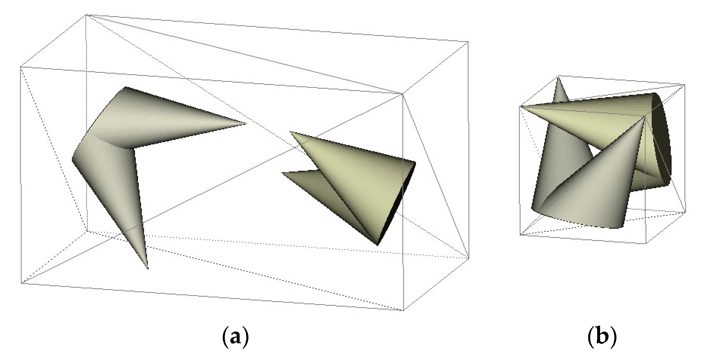
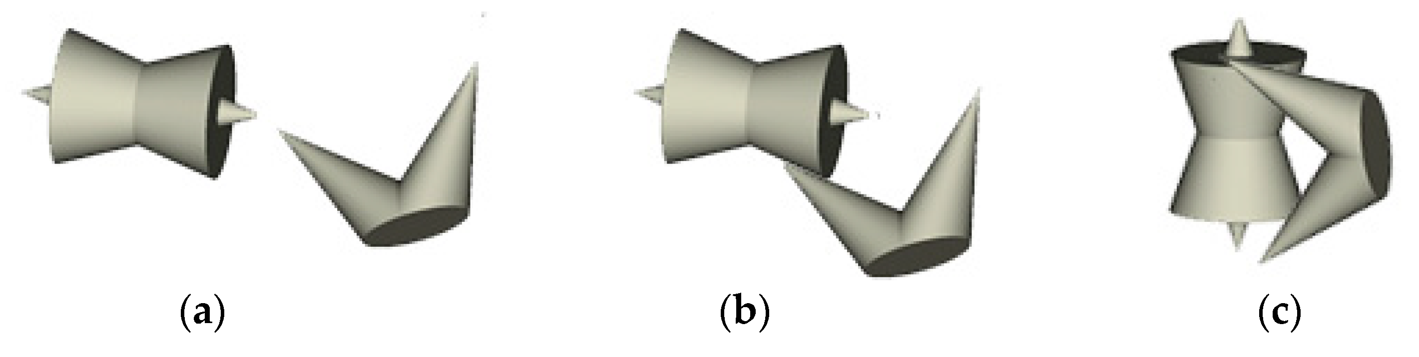
Example 1.

The optimized packings of $N=25$ irregular objects. Each object $T_q(u_q),q=1,\dots ,25$is composed by the union of two cones$T_i^q(u_q),i=1,2$given by the following parameters:$p_{11}^q=$ (0,0,0), $p_{12}^q=$ (9,0,0), $n_1^q=$ (1,0,0), $r_{11}^q=$ 3, $r_{12}^q=$ 0 and $p_{21}^q=$ (7,0,0), $p_{22}^q=$ (−2,0,0), $n_2^q=$ (1,0,0), $r_{21}^q=$ 3, $r_{22}^q=$ 0 respectively.

The best local minimum obtained for 2857.99 sec is ${\mathsf{\kappa }}^{*}=l^{*}\cdot w^{*}\cdot h^{*}=17.673918\cdot 20.065788\cdot 24.972631=8856.3211208954$.

The corresponding packing is shown in Figure 4a.

Example 2.

The optimized packings of$N=25$basic and irregular objects, including:

−

spheres$T_q(u_q),q=1,\dots ,10$of radii$r_{}^q=$ 2 centred at $p_{}^q=$ (0,0,0);

−

irregular objects$T_q(u_q),q=11,\dots ,15$composed by the union of three basic objects$T_i^q(u_q),i=1,2,3$, where$T_1^q(u_q)$is the cylinder with$p_{11}^q=$ (0,0,0), $p_{12}^q=$ (8,0,0), $n_1^q=$ (1,0, 0), $r_{11}^q=$ 2, $r_{12}^q=$ 2; $T_2^q(u_q)$ and $T_3^q(u_q)$ are the spheres of radii $r_2^q=r_3^q=$ 3, centred at the points $p_2^q=p_3^q=$ (0,0, 0);

−

irregular objects $T_q(u_q),q=16,\dots ,20$ composed by the union of two basic objects $T_i^q(u_q),i=1,2$, where $T_1^q(u_q)$ is the truncated cone with$p_{11}^q=$ (0,0,0), $p_{12}^q=$ (9,0,0), $n_1^q=$ (1,0,0), $r_{11}^q=$ 1, $r_{12}^q=$ 3; $T_2^q(u_q)$ is the cone with $p_{21}^q=$ (0,0,0), $p_{22}^q=$ (9,0,0), $n_2^q=$ (1,0,0), $r_{21}^q=$ 3, $r_{22}^q=$ 0;

−

irregular objects $T_q(u_q),q=21,\dots ,25$ composed by the union of two cones $T_i^q(u_q),i=1,2$ with$p_{11}^q=$ (0,0,0), $p_{12}^q=$ (8,6,0), $n_1^q=$ (1,0,0), $r_{11}^q=$ 3, $r_{12}^q=$ 0; $p_{21}^q=$ (0,0,0), $p_{22}^q=$ (8,6,0), $n_2^q=$ (1,0,0), $r_{21}^q=$ 3, $r_{22}^q=$ 0 respectively.

The best local minimum obtained for 3478.23 sec. is ${\mathsf{\kappa }}^{*}=l^{*}\cdot w^{*}\cdot h^{*}=14.889393\cdot 24.925430\cdot 17.165791=6370.6459961746$.

The corresponding packing is shown in Figure 4b.

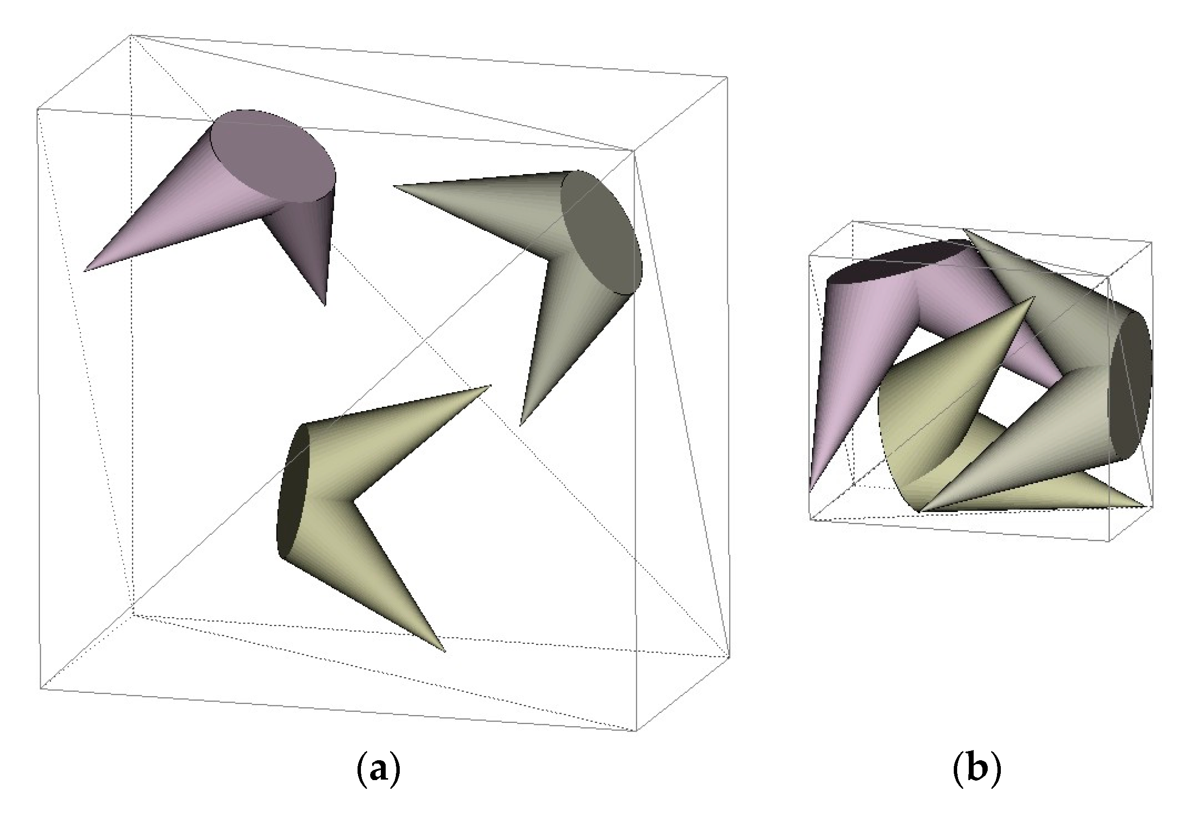
Example 3.

The optimized packings of$N=2,3,4,5$objects from Example 1:

(1)

for$N=2$the best local minimum

$${\mathsf{\kappa }}^{*}=l^{*}\cdot w^{*}\cdot h^{*}=8.085071\cdot 10.392305\cdot 6.000000=504.135155$$

was obtained for 11.638 sec. starting from the feasible solution

$${\mathsf{\kappa }}^0=l^0\cdot w^0\cdot h^0=26.147623\cdot 14.547834\cdot 14.550066=5534.7182137988.$$

The corresponding packings are shown in Figure 5.

(2)

for$N=3$the best local minimum

$${\mathsf{\kappa }}^{*}=l^{*}\cdot w^{*}\cdot h^{*}=12.682284\cdot 11.050980\cdot 6.000000=840.910031$$

was obtained for 26.146 sec. starting from the feasible solution

$${\mathsf{\kappa }}^0=l^0\cdot w^0\cdot h^0=27.617932\cdot 26.392891\cdot 13.953370=10170.849561976.$$

The corresponding packings are shown in Figure 6.

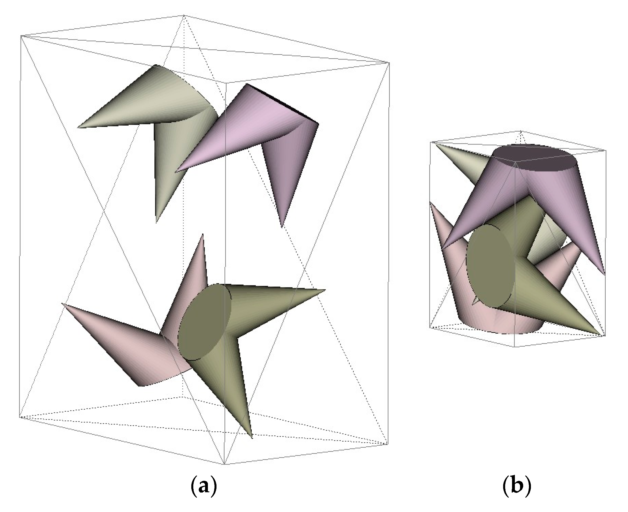
(3)

for$N=4$the best local minimum

$${\mathsf{\kappa }}^{*}=l^{*}\cdot w^{*}\cdot h^{*}=8.091432\cdot 13.454112\cdot 10.099594=1099.4724285295$$

was obtained for 53.602 sec. starting from the feasible solution

$${\mathsf{\kappa }}^0=l^0\cdot w^0\cdot h^0=14.771808\cdot 27.984482\cdot 24.620742=10177.75667595.$$

The corresponding packings are shown in Figure 7.

(4)

for$N=5$the best local minimum

$${\mathsf{\kappa }}^{*}=l^{*}\cdot w^{*}\cdot h^{*}=11.492738\cdot 11.267728\cdot 10.652737=1379.4979707504$$

was obtained for 79.186 sec. starting from the feasible solution

$${\mathsf{\kappa }}^0=l^0\cdot w^0\cdot h^0=26.126900\cdot 26.524042\cdot 23.378807=16201.302676444.$$

The corresponding packings are shown in Figure 8.

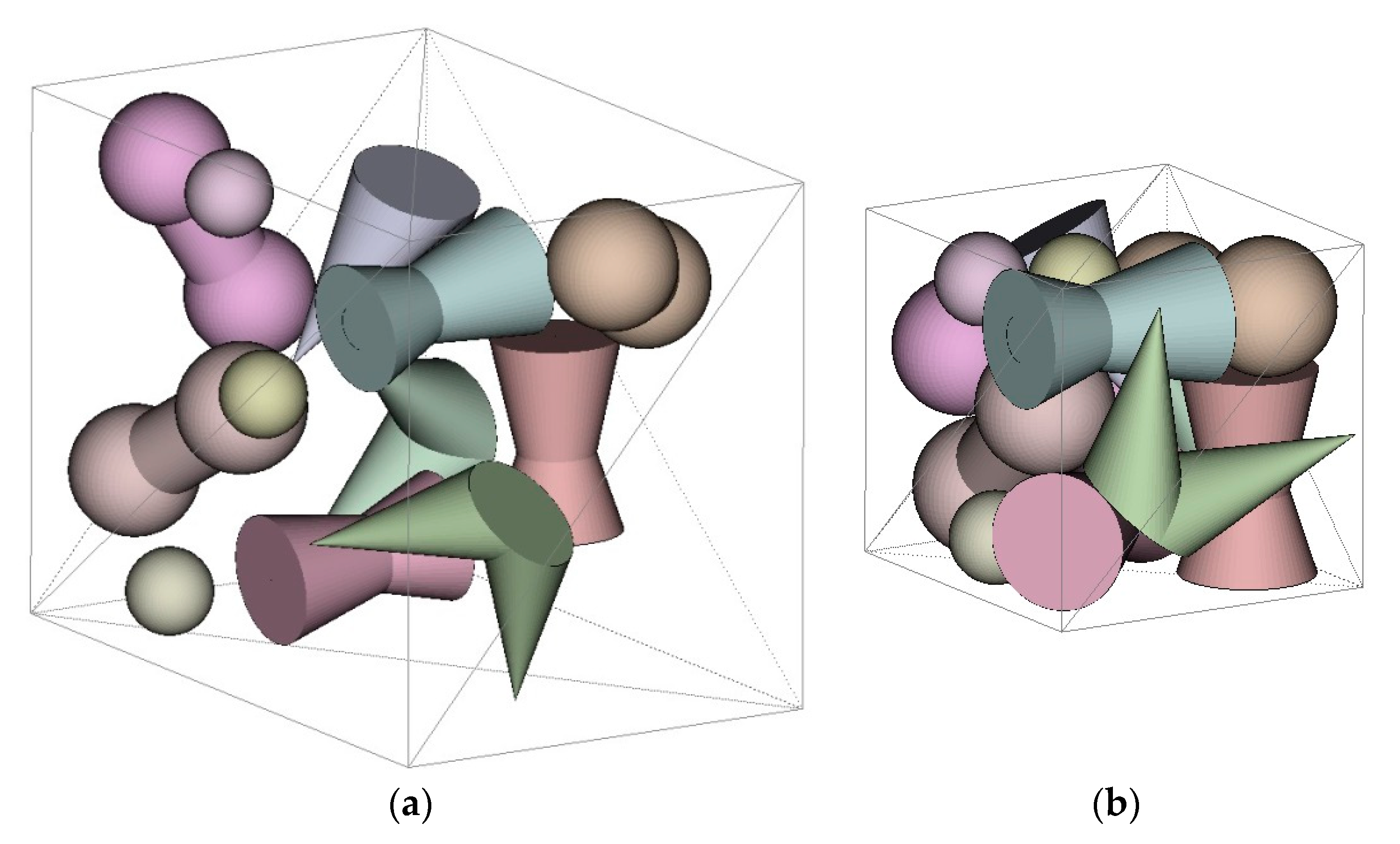
Example 4.

The optimized packings of$N=12$objects (three objects of each type from Example 2).

The best local minimum

$${\mathsf{\kappa }}^{*}=l^{*}\cdot w^{*}\cdot h^{*}=15.084109\cdot 15.073729\cdot 16.129947=3667.5268798149$$

was obtained for 934.103 sec. starting from the feasible solution

$${\mathsf{\kappa }}^0=l^0\cdot w^0\cdot h^0=20.944159\cdot 24.547251\cdot 32.847595=16887.65573111.$$

The corresponding packings are shown in Figure 9.

Table 1. Objective values for feasible starting points and corresponding local optima.

	N = 2		N = 3		N = 4		N = 5		N = 12
	${\mathit{\kappa }}^0$	${\mathit{\kappa }}^{*}$	${\mathit{\kappa }}^0$	${\mathit{\kappa }}^{*}$	${\mathit{\kappa }}^0$	${\mathit{\kappa }}^{*}$	${\mathit{\kappa }}^0$	${\mathit{\kappa }}^{*}$	${\mathit{\kappa }}^0$	${\mathit{\kappa }}^{*}$
1	5337.97	816.30	10,170.84	840.91	11,077.98	1565.10	15,543.36	1536.67	18,810.97	4132.31
2	5215.23	835.79	8733.59	1118.40	12,479.28	1372.18	15,564.86	1639.94	18,886.64	4039.23
3	5580.59	1002.95	9085.77	1319.98	10,011.8	1668.54	15,415.77	1507.72	16,951.12	4014.97
4	5457.55	670.08	9949.29	1145.73	10,177.75	1099.47	16,201.30	1379.50	16,708.20	4478.20
5	5534.71	504.13	9029.34	1063.02	12,348.53	1214.28	15,253.70	1920.94	16,726.72	4160.61
6	5260.31	670.08	9801.35	1409.52	17,169.69	1365.29	16,085.74	1733.08	16,480.82	4055.20
7	5395.85	767.15	10,148.29	1152.08	11,556.14	1826.22	15,634.75	1398.68	16,887.65	3667.53
8	5403.27	1091.65	12,206.66	1134.85	10,317.50	1597.13	17,578.42	1670.72	17,137.79	4102.02
9	5332.57	761.25	12,003.17	1094.66	12,295.11	1264.55	17,556.03	1682.84	17,311.19	3809.62
10	4787.59	896.41	9634.21	1426.20	12,860.21	1637.15	15,228.21	1800.38	15,868.61	3879.69

below provides objective function values for the feasible starting point (${\kappa }^0$) and the corresponding local optimal solution (${\kappa }^{*}$) for all 10 starting points. These values are indicated for N = 2, 3, 4, 5 (Example 3) and N = 12 (Example 4). The best local optimal solutions are highlighted in bold.

As can be seen from Table 1, different starting points lead to different local minima.

6. Conclusions

Packing irregular 3D objects in a cuboid of minimum volume is considered. Each irregular object is composed by convex shapes from the family of oblique and right circular cylinders, cones, truncated cones and spheres. Continuous translations and rotations for all objects are allowed. The optimized packing problem is formulated for 3D regular and irregular objects. New analytical tools (quasi-phi-functions and phi-functions) are defined for the first time to describe non-overlapping and containment constraints for irregular objects composed by oblique shapes.

The phi-function technique is used to state the irregular packing in the form of nonlinear programming problem. The solution approach is proposed and illustrated by the numerical examples. The problem instances were selected to demonstrate the ability of the proposed modelling techniques to work with complex objects composed by different convex shapes used in applications.

The multistart algorithm used in this paper consists of two stages: constructing a number of initial feasible solutions and using local minimization (compaction) procedure to improve starting points. A simple and fast heuristic was implemented to get a starting solution. Using more advanced heuristics to construct better starting points may result in improving the overall optimization scheme. Some results in this direction are on the way.

The model (8)–(9) provides all global solutions to the original irregular packing problem. It can be solved by global solvers, e.g., BARON or LGO included in AMPL [46]. However, due to a large number of variables and constraints, the direct solution to this problem is time consuming and this approach was not used in the paper. Instead, the decomposition technique was used for the large-scale problem (8)–(9) and combined with IPOPT for solving NLP subproblems. An interesting direction for the future research is using alternative decomposition techniques [49] or constructing Lagrangian relaxations with respect to binding constraints (see, e.g., [50] and the references therein).

References

- Bortfeldt, A.; Wäscher, G. Constraints in container loading—A state-of-the-art review. Eur. J. Oper. Res. 2013, 229, 1–20. [Google Scholar] [CrossRef]
- Leao, A.A.; Toledo, F.M.; Oliveira, J.F.; Carravilla, M.A.; Alvarez-Valdés, R. Irregular packing problems: A review of mathematical models. Eur. J. Oper. Res. 2020, 282, 803–822. [Google Scholar] [CrossRef]
- Chazelle, B.; Edelsbrunner, H.; Guibas, L.J. The complexity of cutting complexes. Discret. Comput. Geom. 1989, 4, 139–181. [Google Scholar] [CrossRef]
- Wäscher, G.; Haußner, H.; Schumann, H. An improved typology of cutting and packing problems. Eur. J. Oper. Res. 2007, 183, 1109–1130. [Google Scholar] [CrossRef]
- Burtseva, L.; Salas, B.V.; Romero, R.; Werner, F. Multi-Sized Sphere Packings: Models and Recent Approaches [Preprint]; Fakultät für Mathematik, Otto-von-Guericke-Universität Magdeburg: Magdeburg, Germany, 2015. [Google Scholar] [CrossRef]
- Burtseva, L.; Salas, B.V.; Romero, R.; Werner, F. Recent advances on modelling of structures of multi-component mixtures using a sphere packing approach. Int. J. Nanotechnol. 2016, 13, 44. [Google Scholar] [CrossRef]
- Fasano, G.; Pintér, J.D. Modeling and optimization with case studies. In Springer Optimization and Its Applications: Space Engineering; Springer: New York, NY, USA, 2016; Volume 114. [Google Scholar] [CrossRef]
- Gately, R.D.; Panhuis, M.I.H. Filling of carbon nanotubes and nanofibres. Beilstein J. Nanotechnol. 2015, 6, 508–516. [Google Scholar] [CrossRef] [Green Version]
- Ungson, Y.; Burtseva, L.; Garcia-Curiel, E.R.; Salas, B.V.; Flores-Rios, B.L.; Werner, F.; Petranovskii, V. Filling of irregular channels with round cross-section: Modeling aspects to study the properties of porous materials. Materials 2018, 11, 1901. [Google Scholar] [CrossRef] [Green Version]
- Araújo, L.J.; Özcan, E.; Atkin, J.; Baumers, M. Analysis of irregular three-dimensional packing problems in additive manufacturing: A new taxonomy and dataset. Int. J. Prod. Res. 2018, 57, 5920–5934. [Google Scholar] [CrossRef]
- Stoyan, Y.; Панкратов, A.B.; Romanova, T.; Butenko, S.; Pardalos, P.M.; Shylo, V. Placement problems for irregular objects: Mathematical modeling, optimization and applications. Springer Texts Stat. 2017, 130, 521–559. [Google Scholar] [CrossRef]
- Romanova, T.; Bennell, J.; Stoyan, Y.; Панкратов, A.B. Packing of concave polyhedra with continuous rotations using nonlinear optimisation. Eur. J. Oper. Res. 2018, 268, 37–53. [Google Scholar] [CrossRef]
- Kovalenko, A.; Romanova, T.; Stetsyuk, P. Balance Layout Problem for 3D-Objects: Mathematical Model and Solution Methods. Cybern. Syst. Anal. 2015, 51, 556–565. [Google Scholar] [CrossRef]
- Edelkamp, S.; Wichern, P. Packing irregular-shaped objects for 3D Printing. In KI: Advances in Artificial Intelligence; Springer: Cham, Switzerland, 2015; Volume 9324, pp. 45–58. [Google Scholar]
- Romanova, T.; Litvinchev, I.; Pankratov, A. Packing ellipsoids in an optimized cylinder. Eur. J. Oper. Res. 2020. [CrossRef]
- Romanova, T.; Панкратов, А.В.; Litvinchev, I.; Plankovskyy, S.; Tsegelnyk, Y.; Shypul, O. Sparsest packing of two-dimensional objects. Int. J. Prod. Res. 2020, 1–16. [Google Scholar] [CrossRef]
- Stoyan, Y.; Grebennik, I.; Romanova, T.; Kovalenko, A. Optimized packings in space engineering applications: Part II. In Modeling and Optimization in Space Engineering; Springer International Publishing: New York, NY, USA, 2019; Volume 144, pp. 439–457. [Google Scholar]
- Stoyan, Y.; Pankratov, A.; Romanova, T.; Fasano, G.; Pintér, J.D.; Stoian, Y.E.; Chugay, A. Optimized packings in space engineering applications: Part I. In Modeling and Optimization in Space Engineering; Springer International Publishing: New York, NY, USA, 2019; Volume 144, pp. 395–437. [Google Scholar] [CrossRef]
- Fasano, G. A Modeling-based approach for non-standard packing problems. In Springer Optimization and Its Applications: Space Engineering; Springer: New York, NY, USA, 2015; Volume 105, pp. 67–85. [Google Scholar] [CrossRef]
- Hifi, M.; Yousef, L. A local search-based method for sphere packing problems. Eur. J. Oper. Res. 2019, 274, 482–500. [Google Scholar] [CrossRef]
- Pintér, J.D.; Kampas, F.J.; Castillo, I. Globally optimized packings of non-uniform size spheres in Rd: A computational study. Optim. Lett. 2017, 12, 585–613. [Google Scholar] [CrossRef]
- Litvinchev, I.; Infante, L.; Ozuna Espinosa, E.L. Approximate Circle Packing in a Rectangular Container: Integer Programming Formulations and Valid Inequalities. In Proceedings of the International Conference on Computational Logistics, ICCL, Valparaíso, Chile, 24–26 September 2014; González-Ramírez, R.G., Schulte, F., Voß, S., Ceroni Díaz, J.A., Eds.; Springer: Cham, Switzerland, 2014; Volume 8760, pp. 47–60. [Google Scholar]
- Depriester, D.; Kubler, R. Radical Voronoï tessellation from random pack of polydisperse spheres: Prediction of the cells’ size distribution. Comput. Des. 2019, 107, 37–49. [Google Scholar] [CrossRef]
- Lucarini, V. Three-Dimensional Random Voronoi Tessellations: From Cubic Crystal Lattices to Poisson Point Processes. J. Stat. Phys. 2009, 134, 185–206. [Google Scholar] [CrossRef]
- Pankratov, A.; Romanova, T.; Litvinchev, I.; Marmolejo-Saucedo, J.A. An Optimized Covering Spheroids by Spheres. Appl. Sci. 2020, 10, 1846. [Google Scholar] [CrossRef] [Green Version]
- Zhao, B.; An, X.; Wang, Y.; Qian, Q.; Yang, X.; Sun, X. DEM dynamic simulation of tetrahedral particle packing under 3D mechanical vibration. Powder Technol. 2017, 317, 171–180. [Google Scholar] [CrossRef]
- Wang, X.; Zhao, L.; Fuh, J.Y.H.; Lee, H.P. Lee effect of porosity on mechanical properties of 3D Printed polymers: Experiments and micromechanical modeling based on X-Ray computed tomography analysis. Polymers 2019, 11, 1154. [Google Scholar] [CrossRef] [Green Version]
- Egeblad, J.; Nielsen, B.K.; Brazil, M. Translational packing of arbitrary polytopes. Comput. Geom. 2009, 42, 269–288. [Google Scholar] [CrossRef] [Green Version]
- Gogate, A.S.; Pande, S.S. Intelligent layout planning for rapid prototyping. Int. J. Prod. Res. 2008, 46, 5607–5631. [Google Scholar] [CrossRef]
- Joung, Y.-K.; Noh, S.D. Intelligent 3D packing using a grouping algorithm for automotive container engineering. J. Comput. Des. Eng. 2014, 1, 140–151. [Google Scholar] [CrossRef] [Green Version]
- Mack, D.; Bortfeldt, A.; Gehring, H. A parallel hybrid local search algorithm for the container loading problem. Int. Trans. Oper. Res. 2004, 11, 511–533. [Google Scholar] [CrossRef]
- Liu, X.; Liu, J.-M.; Cao, A.-X.; Yao, Z.-L. HAPE3D—A new constructive algorithm for the 3D irregular packing problem. Front. Inf. Technol. Electron. Eng. 2015, 16, 380–390. [Google Scholar] [CrossRef]
- Lutters, E.; Dam, D.T.; Faneker, T. 3D nesting of complex shapes. Procedia CIRP 2012, 3, 26–31. [Google Scholar] [CrossRef] [Green Version]
- Bortfeldt, A.; Gehring, H. A hybrid genetic algorithm for the container loading problem. Eur. J. Oper. Res. 2001, 131, 143–161. [Google Scholar] [CrossRef]
- Gehring, H.; Bortfeldt, A. A Parallel genetic algorithm for solving the container loading problem. Int. Trans. Oper. Res. 2002, 9, 497–511. [Google Scholar] [CrossRef]
- Ma, Y.; Chen, Z.; Hu, W.; Wang, W. Packing irregular objects in 3D space via hybrid optimization. Comput. Graph. Forum 2018, 37, 49–59. [Google Scholar] [CrossRef]
- Zhao, C.; Jiang, L.; Teo, K.L. A hybrid chaos firefly algorithm for three-dimensional irregular packing problem. J. Ind. Manag. Optim. 2020, 16, 409–429. [Google Scholar] [CrossRef] [Green Version]
- Chernov, N.; Stoyan, Y.; Romanova, T. Mathematical model and efficient algorithms for object packing problem. Comput. Geom. 2010, 43, 535–553. [Google Scholar] [CrossRef] [Green Version]
- You, Y.; Zhao, Y. Discrete element modelling of ellipsoidal particles using super-ellipsoids and multi-spheres: A comparative study. Powder Technol. 2018, 331, 179–191. [Google Scholar] [CrossRef]
- Garboczi, E.; Bullard, J. 3D analytical mathematical models of random star-shape particles via a combination of X-ray computed microtomography and spherical harmonic analysis. Adv. Powder Technol. 2017, 28, 325–339. [Google Scholar] [CrossRef] [Green Version]
- Wang, S.; Marmysh, D.; Ji, S. Construction of irregular particles with superquadric equation in DEM. Theor. Appl. Mech. Lett. 2020, 10, 68–73. [Google Scholar] [CrossRef]
- Rakotonirina, A.D.; Delenne, J.-Y.; Radjaï, F.; Wachs, A. Grains3D, a flexible DEM approach for particles of arbitrary convex shape—Part III: Extension to non-convex particles modelled as glued convex particles. Comput. Part. Mech. 2018, 6, 55–84. [Google Scholar] [CrossRef] [Green Version]
- Gibson, I.; Rosen, D.; Stucker, B. Additive Manufacturing Technologies, 3D Printing, Rapid Prototyping, and Direct Digital Manufacturing; Springer Science + Business Media: New York, NY, USA, 2015; ISBN 978-1-4939-2113-3. [Google Scholar]
- Yuan, Y.; Liu, L.; Deng, W.; Li, S. Random-packing properties of spheropolyhedra. Powder Technol. 2019, 351, 186–194. [Google Scholar] [CrossRef]
- Wei, G.; Zhang, H.; An, X.; Jiang, S. Influence of particle shape on microstructure and heat transfer characteristics in blast furnace raceway with CFD-DEM approach. Powder Technol. 2020, 361, 283–296. [Google Scholar] [CrossRef]
- Robert, F.; Gay, D.M.; Brian, W. Kernighan, AMPL: A Modeling Language for Mathematical Programming, 2nd ed.; Pacific Grove: New York, NY, USA, 2003. [Google Scholar]
- Romanova, T.; Stoyan, Y.G.; Pankratov, A.V.; Litvinchev, I.; Marmolejo-Saucedo, J.A. Decomposition algorithm for irregular placement problems. In Advances in Intelligent Systems and Computing; Springer Nature Switzerland AG: Cham, Switzerland, 2019; pp. 214–221. [Google Scholar]
- Wächter, A.; Biegler, L.T. On the implementation of an interior-point filter line-search algorithm for large-scale nonlinear programming. Math. Program. 2006, 106, 25–57. [Google Scholar] [CrossRef]
- Litvinchev, I. Decomposition-aggregation method for convex programming problems. Optimization 1991, 22, 47–56. [Google Scholar] [CrossRef]
- Litvinchev, I.S. Refinement of Lagrangian bounds in optimization problems. Comput. Math. Math. Phys. 2007, 47, 1101–1107. [Google Scholar] [CrossRef]
Figure 1.
Container Ω.
Figure 2.
Placement objects: (a) basic; (b) composed.
Figure 3.
Non-overlapping: (a) convex basic objects and the half space ; (b) convex basic objects and the half space .
Figure 4.
Optimized packings of composed objects: (a) Example 1; (b) Example 2.
Figure 5.
Packings of two composed objects: (a) the feasible starting point; (b) the corresponding local optimal packing.
Figure 6.
Packings of three composed objects: (a) the feasible starting point; (b) the corresponding local optimal packing.
Figure 7.
Packings of four composed objects: (a) the feasible starting point; (b) the corresponding local optimal packing.
Figure 8.
Packings of five composed objects: (a) the feasible starting point; (b) the corresponding local optimal packing.
Figure 9.
Packings of twelve composed objects: (a) the feasible starting point; (b) the corresponding local optimal packing.