Parameter Identification in Nonlinear Mechanical Systems with Noisy Partial State Measurement Using PID-Controller Penalty Functions

Abstract

Dynamic models of physical systems often contain parameters that must be estimated from experimental data. In this work, we consider the identification of parameters in nonlinear mechanical systems given noisy measurements of only some states. The resulting nonlinear optimization problem can be solved efficiently with a gradient-based optimizer, but convergence to a local optimum rather than the global optimum is common. We augment the dynamic equations with a morphing parameter and a proportional–integral–derivative (PID) controller to transform the objective function into a convex function; the global optimum can then be found using a gradient-based optimizer. The morphing parameter is used to gradually remove the PID controller in a sequence of steps, ultimately returning the model to its original form. An optimization problem is solved at each step, using the solution from the previous step as the initial guess. This strategy enables use of a gradient-based optimizer while avoiding convergence to a local optimum. The efficacy of the proposed approach is demonstrated by identifying parameters in the van der Pol–Duffing oscillator, a hydraulic engine mount system, and a magnetorheological damper system. Our method outperforms genetic algorithm and particle swarm optimization strategies, and demonstrates robustness to measurement noise.

1. Introduction

To generate a simulation of a mechanical system, one first requires a mathematical model of the system’s dynamics. The parameters for dynamic system models are often estimated from experimental measurements, a process called parameter estimation or parameter identification. This task is difficult in general, particularly when the mathematical model is nonlinear. Additional challenges are presented when only some of the system’s states are measured and when experimental data are corrupted by measurement noise. Parameter identification with partial state measurement is highly relevant in many areas of the biological and physical sciences [1].

Parameter identification is typically approached as a least-squares optimization problem, wherein the model parameters must be determined so as to minimize the difference between the measured response of the physical system and the simulated response of the analogous mathematical model [2,3]. Classical optimization techniques include the Gauss–Newton and Levenberg–Marquardt algorithms. These gradient-based methods are very effective provided the objective function is convex; if it is not, they often converge to a local optimum rather than the global optimum [4]. In many mathematical models, the parameters appear nonlinearly with respect to the system states and the objective function is non-convex (i.e., it contains many local optima). Stochastic optimization techniques such as simulated annealing, the genetic algorithm (GA), and particle swarm optimization (PSO) are capable of finding the globally optimal solution to a non-convex problem; however, if a large number of parameters must be identified, these methods tend to become computationally expensive [5,6]. In general, parameter identification problems can be solved more efficiently if a gradient-based algorithm can be used even for non-convex optimization problems.

Homotopy methods have led to effective global optimization algorithms [7]. Vyasarayani et al. explored the application of homotopy optimization to identifying parameters in nonlinear systems, including those governed by differential algebraic equations [8]. In the homotopy optimization method, a high-gain observer and a morphing parameter are introduced into the dynamic equations (and, thus, into the objective function implicitly). This transformation makes the objective function convex [9] and enables use of a gradient-based optimization method. The dynamic equations are gradually morphed back to the original system by reducing the value of the morphing parameter in a sequence of steps. A new optimization problem is solved at each step, using the solution from the previous step as the initial guess. Provided the morphing parameter is reduced in sufficiently small steps, convergence to a local optimum is avoided despite using a simple gradient-based optimizer. This process is continued until the morphing parameter reaches zero, thereby recovering the original optimization problem, but now it is solved starting from a good initial guess.

In the present work, we use a proportional–integral–derivative (PID) controller to implement a homotopy optimization strategy and study the effectiveness of this approach at identifying parameters in the van der Pol–Duffing oscillator, a hydraulic engine mount system, and a magnetorheological (MR) damper system. Accurate mathematical models for engine mount and MR damper systems are important tools for engineering analysis, design, and control applications; thus, fast and accurate parameter identification methods are critical. The PID controller used in this work is a natural extension of the Luenberger observer [10]. We consider partial state measurement, wherein experimental measurements for only some of the system states are available, as well as the effect of measurement noise. We also compare the performance of the proposed approach to the performance of popular GA [11,12,13] and PSO [14,15,16] methods.

The remainder of the paper is organized as follows. The proposed parameter identification strategy is presented in Section 2. Numerical examples are presented and discussed in Section 3. Finally, conclusions are provided in Section 4.

2. Methodology

We assume the dynamics of the experimental system are governed by a system of ordinary differential equations, written here in first-order form:

$$\begin{array}{cc}\hfill {\dot{\mathbf{x}}}_{1e}\left(t\right)& ={\mathbf{x}}_{2e}\left(t\right),\hfill \end{array}$$

(1a)

$$\begin{array}{cc}\hfill {\dot{\mathbf{x}}}_{2e}\left(t\right)& =\mathbf{f}\left({\mathbf{x}}_{1e}\left(t\right),{\mathbf{x}}_{2e}\left(t\right),\mathbf{p},t\right),\hfill \end{array}$$

(1b)

where ${\mathbf{x}}_{1e}\left(t\right)\triangleq {\left[x_{1e}\left(t\right),x_{2e}\left(t\right),\dots ,x_{ne}\left(t\right)\right]}^T$ contains the time series of the n position-level states and $\mathbf{p}\triangleq \left[p_1,p_2,\dots ,p_k\right]$ is a vector of the k parameters in the experimental system. In the following, we assume that only one state variable ($x_{1e}\left(t\right)$) is measured; the other states in the experimental system are unobserved. The mathematical model representing the experimental system (Equation (1a), (1b)) is written in an analogous form:

$$\begin{array}{cc}\hfill {\dot{\mathbf{x}}}_1\left(t\right)& ={\mathbf{x}}_2\left(t\right),\hfill \end{array}$$

(2a)

$$\begin{array}{cc}\hfill {\dot{\mathbf{x}}}_2\left(t\right)& =\mathbf{f}\left({\mathbf{x}}_1\left(t\right),{\mathbf{x}}_2\left(t\right),\widehat{\mathbf{p}},t\right),\hfill \end{array}$$

(2b)

where ${\mathbf{x}}_1\left(t\right)\triangleq {\left[x_1(\widehat{\mathbf{p}},t),x_2(\widehat{\mathbf{p}},t),\dots ,x_n(\widehat{\mathbf{p}},t)\right]}^T$. Our notation here emphasizes that the trajectory of the mathematical model is a function of the unknown parameters $\widehat{\mathbf{p}}\triangleq \left[{\widehat{p}}_1,{\widehat{p}}_2,\dots ,{\widehat{p}}_k\right]$. The objective is to identify the parameters in the mathematical model ($\widehat{\mathbf{p}}$ in (Equation (2a), (2b)) to minimize the error between the experimental measurement ($x_{1e}\left(t\right)$) and the corresponding predicted response ($x_1(\widehat{\mathbf{p}},t)$).

2.1. Optimization Strategy

We identify model parameters $\widehat{\mathbf{p}}$ by minimizing the following objective function:

$$J\left(\widehat{\mathbf{p}}\right)=\frac{1}{2}{\int }_0^{t_f}{\left(x_{1e}\left(t\right)-x_1(\widehat{\mathbf{p}},t)\right)}^{2}dt.$$

(3)

In general, this objective function surface will contain many local minima; a naive optimization strategy may lead to any one of them. To avoid convergence to a local minimum, we introduce a morphing parameter ($\lambda$) and a proportional–integral–derivative (PID) controller into the mathematical model (Equation (2a), (2b)):

$$\begin{array}{cc}\hfill {\dot{\mathbf{x}}}_1\left(t\right)& ={\mathbf{x}}_2\left(t\right)+\lambda k_d\left(x_{1e}\left(t\right)-x_1(\widehat{\mathbf{p}},t)\right),\hfill \end{array}$$

(4a)

$$\begin{array}{cc}\hfill {\dot{\mathbf{x}}}_2\left(t\right)& =\mathbf{f}\left({\mathbf{x}}_1\left(t\right),{\mathbf{x}}_2\left(t\right),\widehat{\mathbf{p}},t\right)+\lambda k_p\left(x_{1e}\left(t\right)-x_1(\widehat{\mathbf{p}},t)\right)+\lambda k_i{\int }_0^t{\left(x_{1e}\left(\tau \right)-x_1(\widehat{\mathbf{p}},\tau )\right)}^{2}d\tau ,\hfill \end{array}$$

(4b)

where $k_p$, $k_i$ and $k_d$ are the proportional, integral and derivative gains, respectively, and $x_{1e}\left(t\right)-x_1(\widehat{\mathbf{p}},t)$ is the error we wish to minimize. The controller used here (with $k_i=0$) resembles the Luenberger observer [10] used in the state estimation of linear systems. The predicted response and objective function are now implicit functions of morphing parameter $\lambda$:

$$J(\widehat{\mathbf{p}},\lambda )=\frac{1}{2}{\int }_0^{t_f}{\left(x_{1e}\left(t\right)-x_1(\widehat{\mathbf{p}},\lambda ,t)\right)}^{2}dt.$$

(5)

The optimization process begins by providing an arbitrary initial guess for the parameters and setting morphing parameter $\lambda =1$. Provided the proportional gain ($k_p$) is sufficiently high, the PID controller in Equation (4a), (4b) will make the objective function surface convex [9], thereby enabling use of any gradient-based optimizer. The optimizer uses the objective function $J(\widehat{\mathbf{p}},1)$ to seek values for the model parameters ($\widehat{\mathbf{p}}$) such that the predicted response ($x_1(\widehat{\mathbf{p}},1,t)$) matches the measured response ($x_{1e}\left(t\right)$). We denote the solution from this step ${}^1{\widehat{\mathbf{p}}}^{*}$. We then reduce $\lambda$ by a small amount $\delta$ and minimize $J(\widehat{\mathbf{p}},1-\delta )$, using ${}^1{\widehat{\mathbf{p}}}^{*}$ as the initial guess. The solution from this step (${}^{1-\delta }{\widehat{\mathbf{p}}}^{*}$) is then used as the initial guess for the subsequent step, where $\lambda =1-2\delta$. This process is repeated until $\lambda =0$, whereupon the PID controller vanishes from the mathematical model (Equation (4a), (4b)). In the final step, $\lambda =0$ and the global minimum to the original problem (${}^0{\widehat{\mathbf{p}}}^{*}$) is obtained.

The proposed approach closely resembles the penalty function method. Any constrained optimization problem can be transformed into an unconstrained optimization problem by treating each constraint violation as a penalty. Each penalty i contributes a new term to the objective function, scaled by a weighting parameter $r_i$. Values are selected for each $r_i$ and the optimization problem is solved. If the violation of a constraint from the original problem is too large, the corresponding weighting parameter is increased and the optimization problem is solved again, using the previous solution as the initial guess. This process is continued until all constraint violations are acceptably low. Penalty functions and weighting parameters $r_i$ are analogous to the PID controller and morphing parameter $\lambda$ in Equation (4a), (4b). However, note that the proposed approach is able to find the global optimum, whereas the penalty function method arrives at only a near-optimal solution in general.

2.2. Error Convergence

To gain insight into the error dynamics of the proposed approach, we subtract Equation (4a), (4b) from Equation (1a), (1b) to obtain the following error equation:

$${\ddot{\mathbf{e}}}_1\left(t\right)+\lambda k_d{\dot{\mathbf{e}}}_1\left(t\right)+\lambda k_p{\mathbf{e}}_1\left(t\right)=\mathbf{f}\left({\mathbf{x}}_{1e}\left(t\right),{\mathbf{x}}_{2e}\left(t\right),\mathbf{p},t\right)-\mathbf{f}\left({\mathbf{x}}_1\left(t\right),{\mathbf{x}}_2\left(t\right),\widehat{\mathbf{p}},t\right)-\lambda k_i{\int }_0^t{\mathbf{e}}_1{\left(\tau \right)}^{2}d\tau .$$

(6)

Equation (6) represents a damped second-order system with stiffness $k_p$, damping $k_d$, and an equilibrium point at ${\mathbf{e}}_1=\mathbf{0}$. The $k_p$, $k_i$, and $k_d$ terms affect the error dynamics as seen in a typical PID controller: the proportional gain determines sensitivity to position-level error, the integral gain determines sensitivity to steady-state error, and the derivative gain determines sensitivity to the rate at which the error is changing. (We note that, for the systems presented in this work, the integral term was found to provide only marginal benefit.) For sufficiently high values of $k_p$, the proportional term dominates and will drive the error to zero regardless of discrepancies between the forcing functions on the right-hand side of Equation (6). A proportional gain should be selected at the outset (i.e., when $\lambda =1$) so that the synchronization error [17] is small when the initial guess for the parameter vector is used in the mathematical model (Equation (4a), (4b)).

3. Results

In this section, we identify parameters in the van der Pol–Duffing oscillator, a hydraulic engine mount system, and a magnetorheological damper system. We explore the effect of measurement noise and provide comparisons with two popular stochastic optimizers: the genetic algorithm and particle swarm optimization strategies.

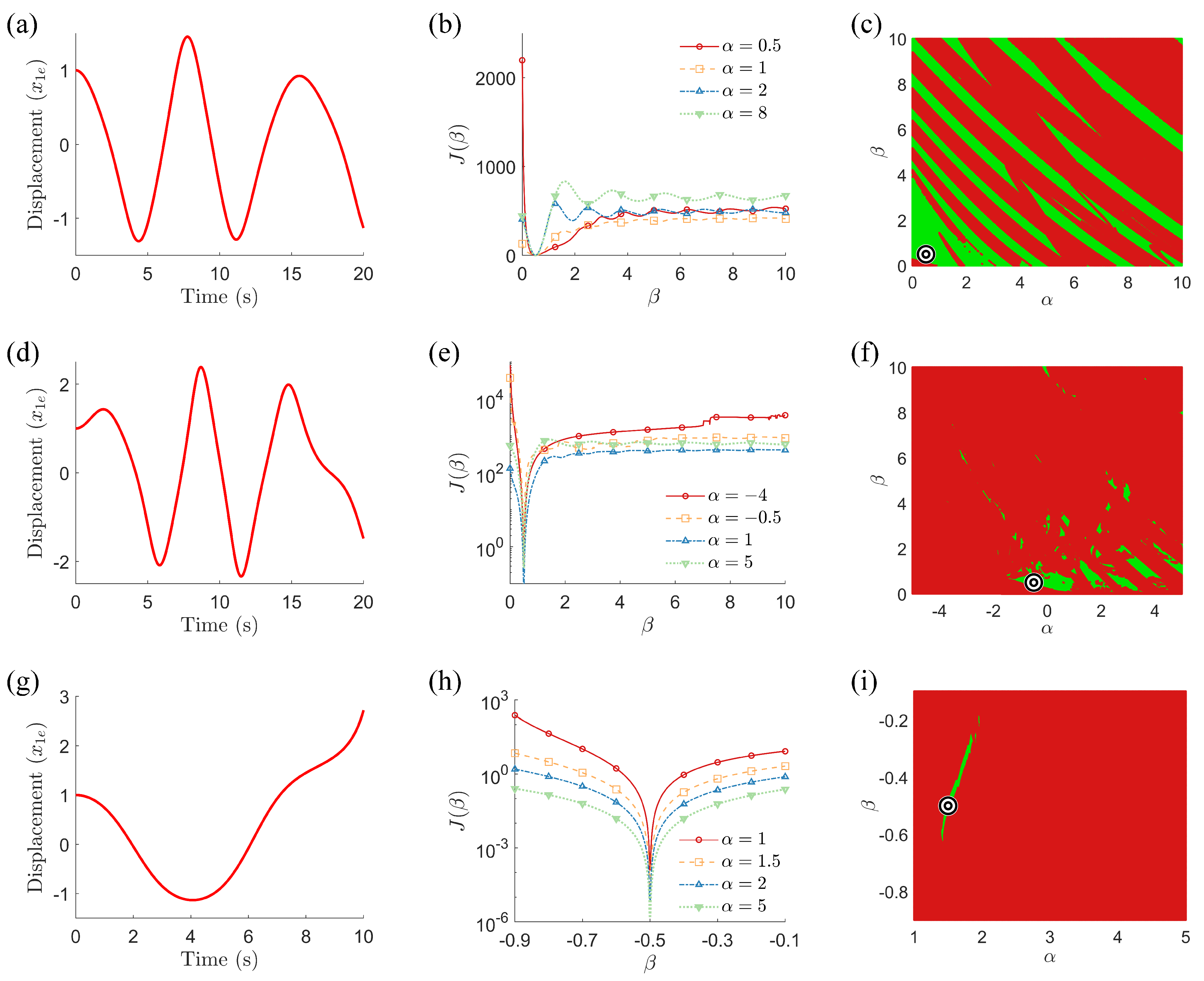
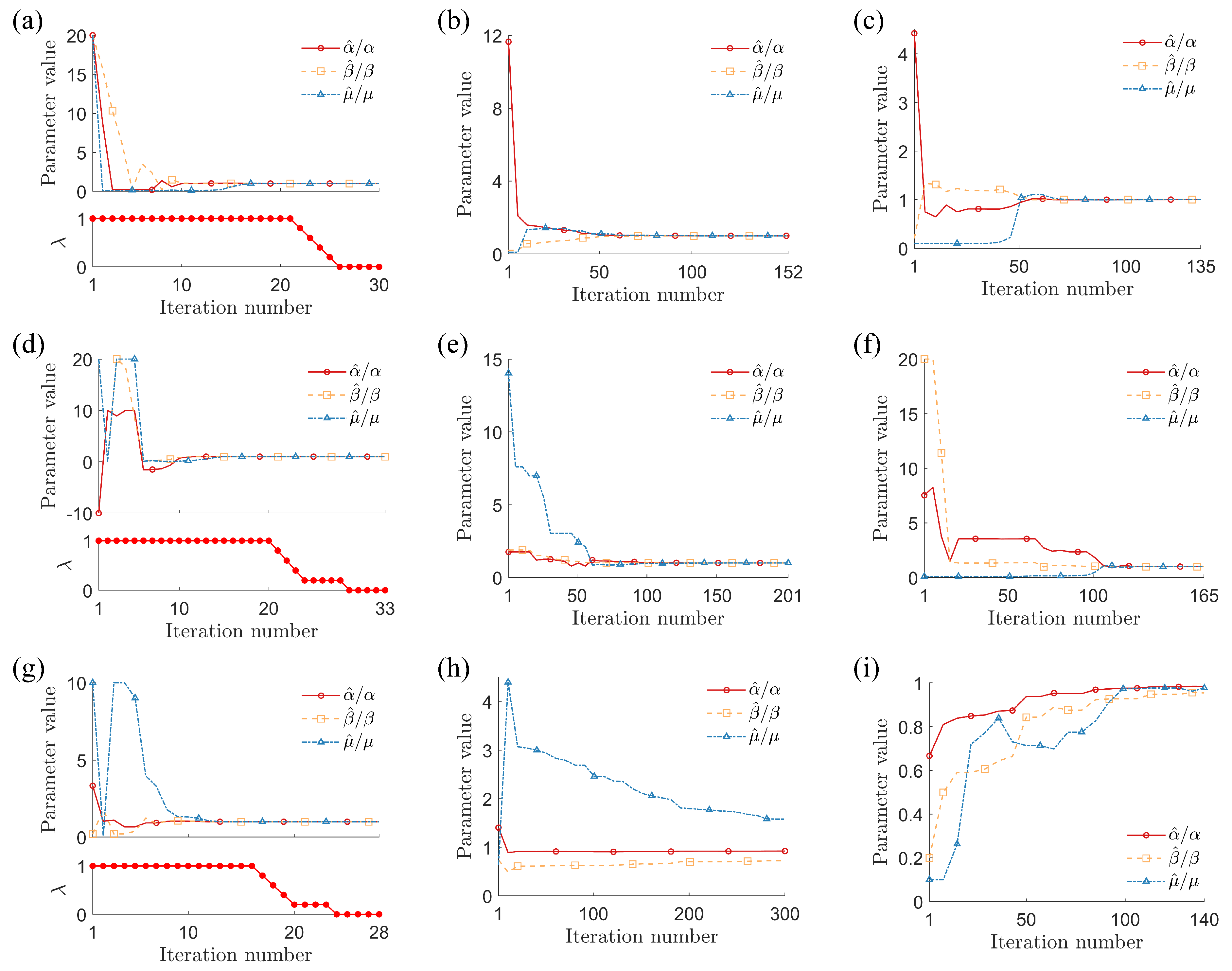
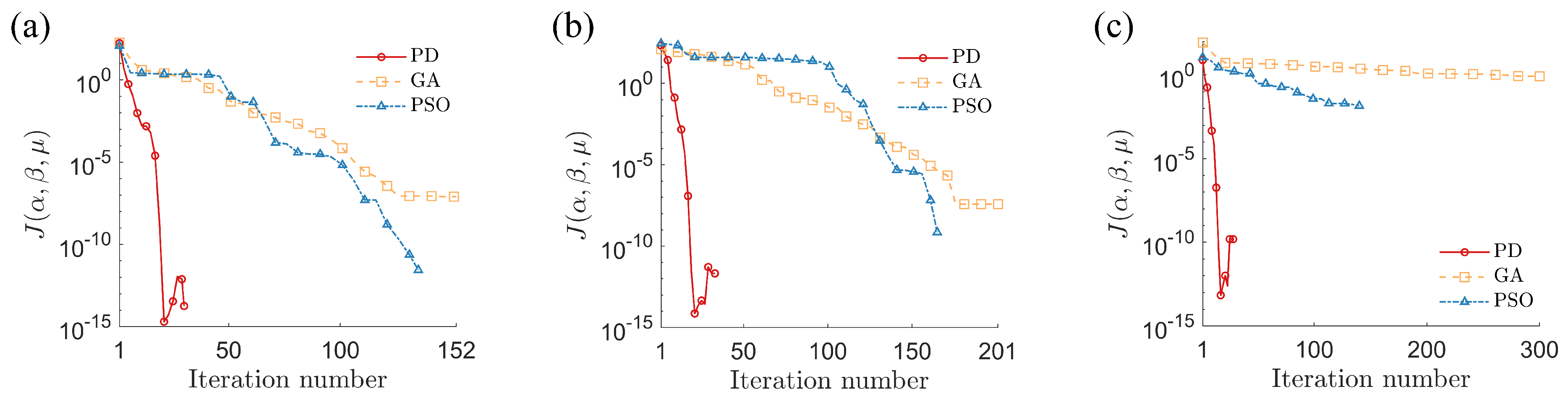
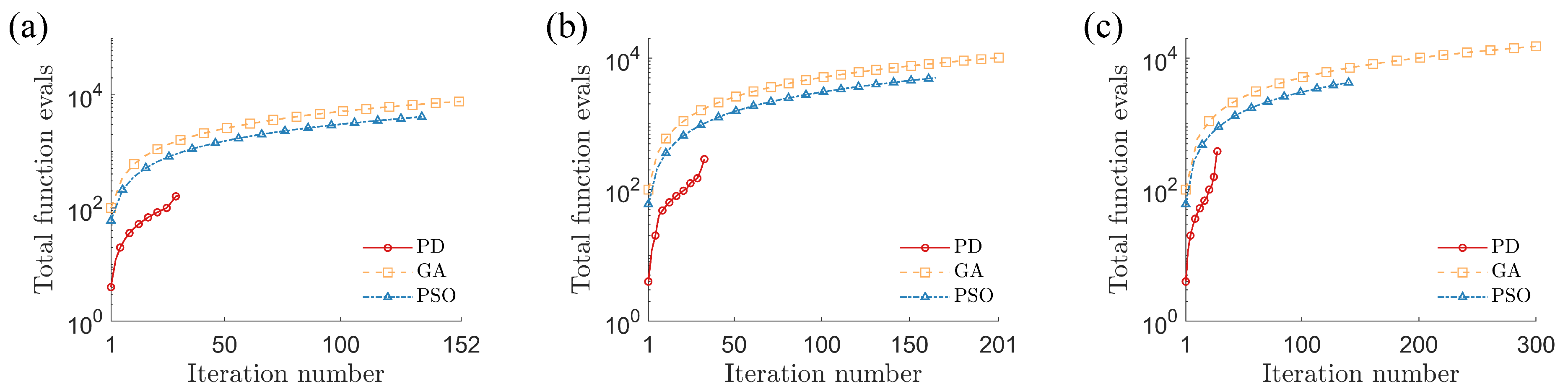
3.1. Van der Pol–Duffing Oscillator

The van der Pol–Duffing (VDPD) oscillator represents a family of classical nonlinear systems with rich dynamical properties, and they appear in many fields of science and engineering [18,19,20,21]. The experimental system we consider in this section is an externally-excited VDPD oscillator [22], given here in first-order form:

$$\begin{array}{cc}\hfill {\dot{x}}_{1e}\left(t\right)& =x_{2e}\left(t\right),\hfill \end{array}$$

(7a)

$$\begin{array}{cc}\hfill {\dot{x}}_{2e}\left(t\right)& =\mu \left(1-x_{1e}^2\left(t\right)\right)x_{2e}\left(t\right)-\alpha x_{1e}\left(t\right)-\beta x_{1e}^3\left(t\right)+f\left(t\right),\hfill \end{array}$$

(7b)

where $f\left(t\right)=gcos\left(\omega t\right)$ is the external excitation, with amplitude $g=0.50$ and frequency $\omega =0.79$. The behavior of the VDPD oscillator depends on three important variables: $\alpha$, $\beta$, and $\mu$. Parameter $\alpha$ determines the stiffness of the system, $\beta$ determines the amount of nonlinearity, and $\mu >0$ is the damping coefficient. VDPD oscillators are typically classified into three categories: single-well ($\alpha$ and $\beta$ both positive), double-well ($\alpha$ negative and $\beta$ positive), and double-hump ($\alpha$ positive and $\beta$ negative). In this example, we seek to identify the system parameters $\alpha$, $\beta$, and $\mu$ given the trajectory of $x_{1e}\left(t\right)$. We assume the initial conditions and the external excitation ($f\left(t\right)$) are known.

As stated in Section 2, we identify parameters for the mathematical model by minimizing Equation (5). In this example, the parameters are $\widehat{\mathbf{p}}\triangleq \left[\widehat{\alpha },\widehat{\beta },\widehat{\mu }\right]$. We assume bounds are known for each parameter; thus, ${\mathbf{p}}^l\le \widehat{\mathbf{p}}\le {\mathbf{p}}^u$ where ${\mathbf{p}}^l$ and ${\mathbf{p}}^u$ are vectors of the lower and upper bounds, respectively. We solve a constrained optimization problem because the VDPD oscillator loses stability beyond particular ranges of parameter values. We consider one experimental system of each category (single-well, double-well, and double-hump); the system parameters and bounds are provided in

Table 1. Experimental parameters and bounds for the van der Pol–Duffing oscillator [22].

Parameter	Single-Well		Double-Well		Double-Hump
	Experimental Value	Bounds	Experimental Value	Bounds	Experimental Value	Bounds
$\alpha$	$0.5$	$\left[0.1,10\right]$	$-0.5$	$\left[-5,5\right]$	$1.5$	$\left[1,5\right]$
$\beta$	$0.5$	$\left[0.1,10\right]$	$0.5$	$\left[0.1,10\right]$	$-0.5$	$\left[-0.9,-0.1\right]$
$\mu$	$0.1$	$\left[0.01,2\right]$	$0.1$	$\left[0.01,2\right]$	$0.1$	$\left[0.01,1\right]$

.

We first consider the single-well case, where the true parameters are $\left[\alpha ,\beta ,\mu \right]=\left[0.5,0.5,0.1\right]$. The initial conditions for the experimental system and mathematical model are assumed to be $\left[x_{1e}\left(0\right),x_{2e}\left(0\right)\right]=\left[x_1\left(0\right),x_2\left(0\right)\right]=\left[1,0\right]$. We generate synthetic experimental data by numerically integrating Equation (7a), (7b) for 20 s [22] using a fourth-order Runge–Kutta method and storing only $x_{1e}\left(t\right)$, as shown in Figure 1a. The shape of the objective function is shown in Figure 1b as a function of $\beta$, for four values of $\alpha$ and with $\mu =0.1$. There are clearly many peaks and valleys in $J\left(\beta \right)$ and, thus, there are many local minima in the objective function $J\left(\widehat{\mathbf{p}}\right)$. We show the basins of attraction in Figure 1c and confirm that a simple gradient-based optimizer is very likely to converge to a local minimum.

To avoid converging to a local minimum, we use the strategy described in Section 2 with a high-gain PD controller. We use initial parameter guesses at the upper bounds, as listed in Table 1 (i.e., $\left[\widehat{\alpha },\widehat{\beta },\widehat{\mu }\right]=\left[10,10,2\right]$) and set $\delta =0.2$. The objective function is given by Equation (5) and is solved using the “fmincon” constrained optimization solver in MATLAB^®; we use the sequential quadratic programming (SQP) algorithm with a first-order optimality tolerance of ${10}^{-6}$ as the termination criterion. The mathematical model is as follows:

$$\begin{array}{cc}\hfill {\dot{x}}_1\left(t\right)& =x_2\left(t\right)+\lambda k_d\left(x_{1e}\left(t\right)-x_1\left(t\right)\right),\hfill \end{array}$$

(8a)

$$\begin{array}{cc}\hfill {\dot{x}}_2\left(t\right)& =\widehat{\mu }\left(1-x_1^2\left(t\right)\right)x_2\left(t\right)-\widehat{\alpha }{x}_1\left(t\right)-\widehat{\beta }{x}_1^3\left(t\right)+f\left(t\right)+\lambda k_p\left(x_{1e}\left(t\right)-x_1\left(t\right)\right).\hfill \end{array}$$

(8b)

Proportional and derivative gains are set to $k_p=k_d=10$, and these values are confirmed to achieve synchronization between the experimental and predicted responses when $\lambda =1$. As shown in Figure 2a, all parameters are successfully identified. The performance of GA and PSO strategies is shown in Figure 2b,c for comparison. We used the “ga” and “pso” functions in MATLAB^® with a population size of 30 in each case (i.e., $10n_p$ where $n_p$ is the number of parameters to be identified [23]). Note that the GA and PSO strategies are also successful at identifying the parameters in the single-well case.

We now repeat the process for double-well and double-hump VDPD oscillators; the experimental data, objective function shape, and basins of attraction for these systems are shown in Figure 1d–i. The double-hump oscillator has a highly unstable response, so we use a simulation duration of 2.5 s in this case. The performance of the PD controller, GA, and PSO strategies is shown in Figure 2d–f for the double-well case and in Figure 2g–i for the double-hump case. All three methods are again successful at identifying the parameters in the double-well case. However, notice that the GA and PSO both fail to find the global optimum in the double-hump case, converging to $\left[\widehat{\alpha },\widehat{\beta },\widehat{\mu }\right]=\left[1.3818,-0.3617,0.1581\right]$ (maximum relative error of 58%) and $\left[1.4754,-0.4767,0.0975\right]$ (maximum relative error of 5%), respectively. Notice the relatively small basin of attraction in Figure 1i, which suggests that the parameter identification problem is relatively challenging in the double-hump case. Even when the GA and PSO strategies are successful, they are substantially more computationally expensive than the proposed PD controller approach. As shown in Figure 3 and Figure 4, the GA and PSO strategies require more iterations and more function evaluations (i.e., they must consider more candidate solutions) than the proposed approach.

Table 2. Performance of optimization strategies for the van der Pol–Duffing oscillator using proportional–derivative controller (PD), genetic algorithm (GA), and particle swarm optimization (PSO) approaches.

Strategy	Single-Well			Double-Well			Double-Hump
	Iter- ations	Function Evals	Error (J)	Iter- ations	Function Evals	Error (J)	Iter- ations	Function Evals	Error (J)
PD	30	165	$1.8\times {10}^{-14}$	33	291	$2.1\times {10}^{-12}$	28	383	$1.5\times {10}^{-10}$
GA	152	7650	$8.1\times {10}^{-8}$	201	10,100	$3.8\times {10}^{-8}$	300	15,050	$0.84$
PSO	135	4080	$2.7\times {10}^{-12}$	165	4980	$7.0\times {10}^{-10}$	140	4230	$0.014$

summarizes the performance of the three strategies.

Finally, we consider the robustness of the proposed approach to uncertainty in the measured data, since experimental measurements are typically corrupted by some amount of noise. We apply Gaussian noise to each data point in the experimental response as follows:

$${\tilde{x}}_{1e}=\left(1+\mathrm{NSR}·r\right)x_{1e},$$

(9)

where ${\tilde{x}}_{1e}$ is the noise-corrupted measurement, $\mathrm{NSR}$ is the noise-to-signal ratio, and r is a zero-mean, normally-distributed random number. As shown in

Table 3. Performance of proportional–derivative controller optimization strategy for the van der Pol–Duffing oscillator with measurement noise (experimental parameter values shown in parentheses).

Noise-to-Signal Ratio	Single-Well			Double-Well			Double-Hump
	$\widehat{\mathit{\alpha }}$ (0.5)	$\widehat{\mathit{\beta }}$ (0.5)	$\widehat{\mathit{\mu }}$ (0.1)	$\widehat{\mathit{\alpha }}$ (−0.5)	$\widehat{\mathit{\beta }}$ (0.5)	$\widehat{\mathit{\mu }}$ (0.1)	$\widehat{\mathit{\alpha }}$ (1.5)	$\widehat{\mathit{\beta }}$ (−0.5)	$\widehat{\mathit{\mu }}$ (0.1)
$1\%$	$0.5009$	$0.4994$	$0.1000$	$-0.5008$	$0.5001$	$0.0999$	$1.5024$	$-0.5025$	$0.0999$
$2\%$	$0.5007$	$0.5005$	$0.0998$	$-0.5034$	$0.4999$	$0.0994$	$1.4990$	$-0.4999$	$0.0985$
$5\%$	$0.5004$	$0.4974$	$0.1005$	$-0.5066$	$0.5009$	$0.0976$	$1.4923$	$-0.4898$	$0.1040$

, the identified parameters are not substantially affected by zero-mean noise, as would be expected. As shown in Figure 5, the predicted response reliably tracks the experimental measurement with $\mathrm{NSR}=5\%$, suggesting that the proposed approach is robust to measurement noise.

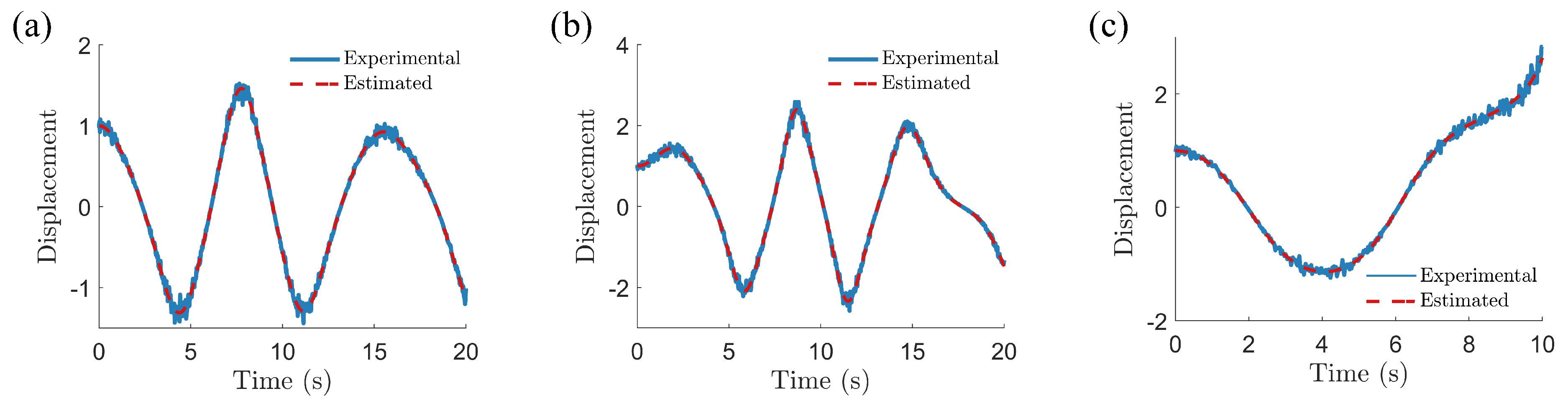
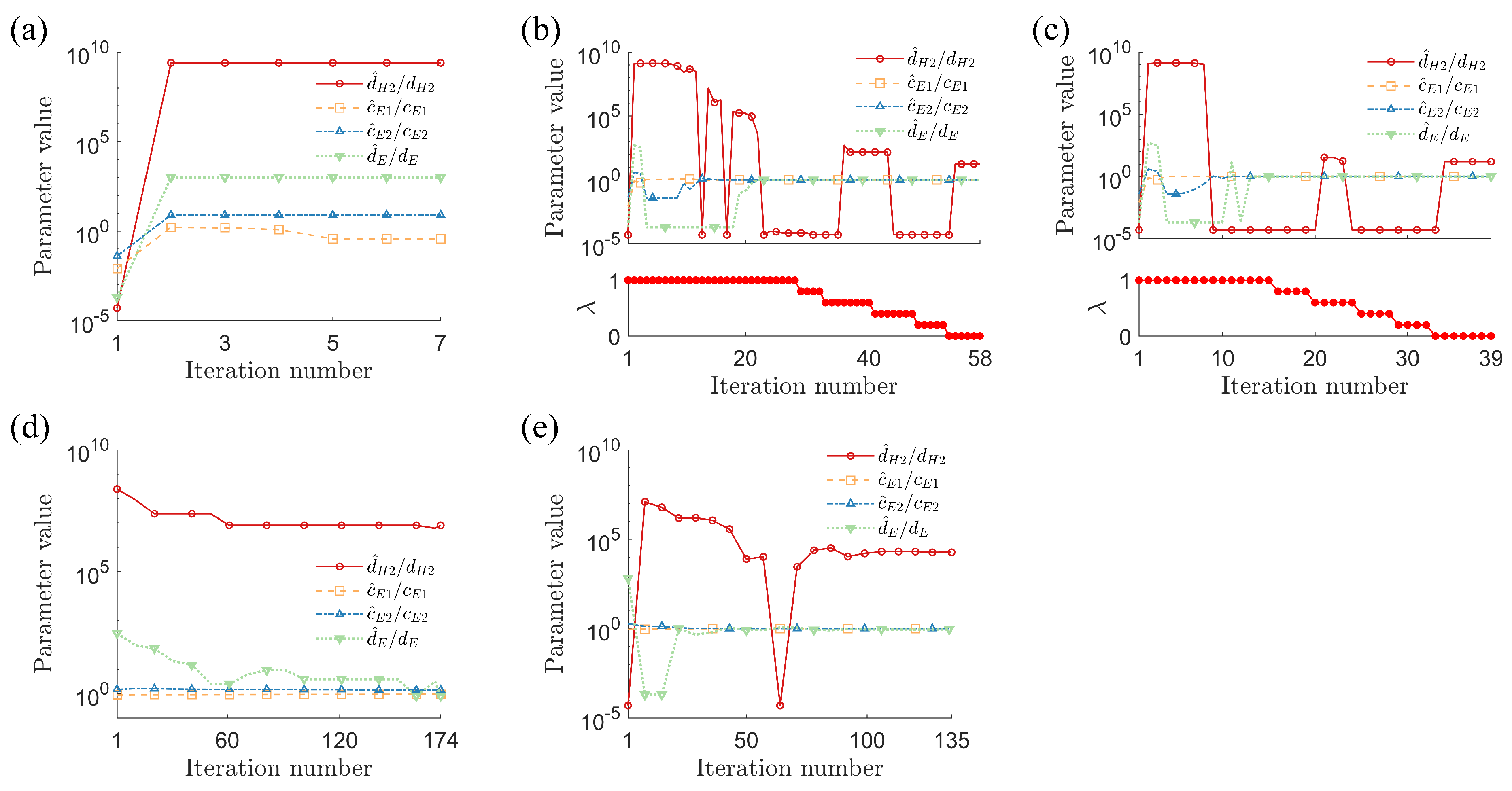
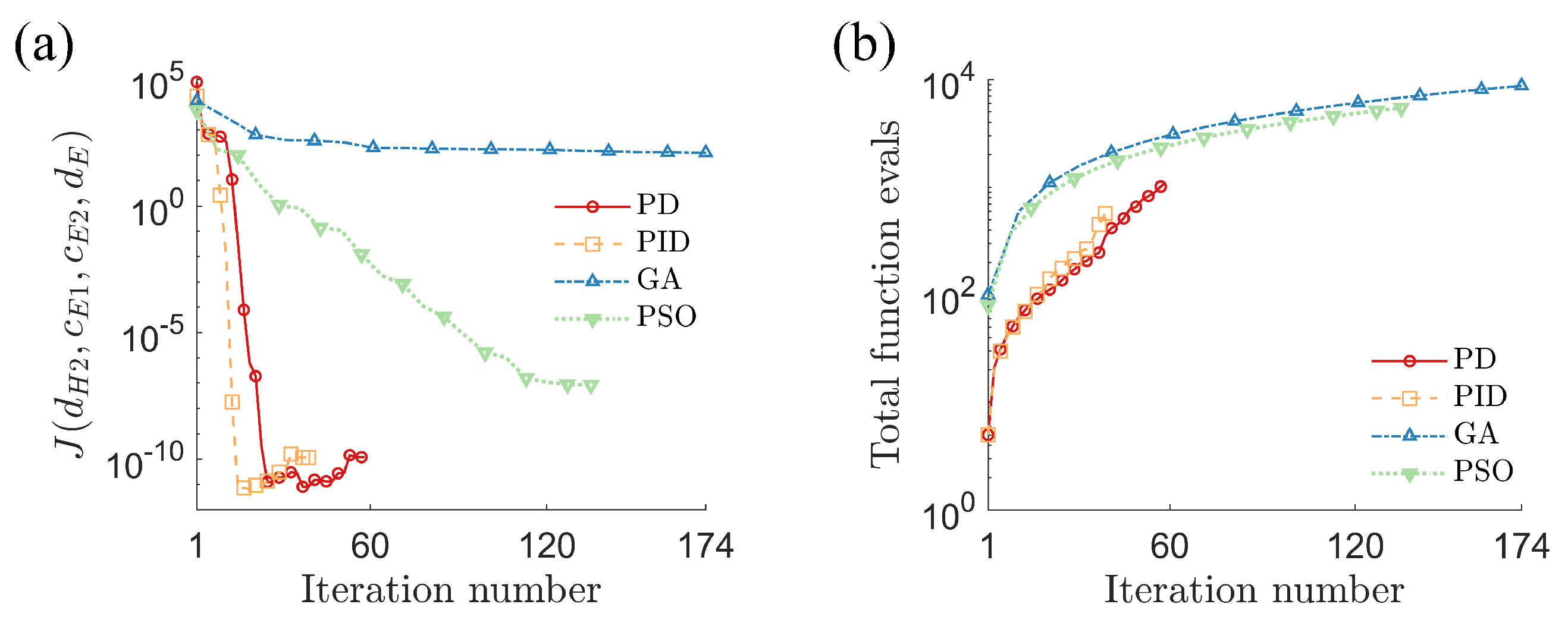
3.2. Hydraulic Engine Mount System

Engine mount systems are designed to isolate passengers in a vehicle from the mechanical vibration of the engine. Designers of these systems must consider two sources of excitation: the low-amplitude, high-frequency vibrations caused by the engine as well as the high-amplitude, low-frequency vibrations induced by the uneven road surface. The response of the engine mount system is critical in the development of engines, and an accurate mathematical model is essential. The mechanical details and operating principles of passive engine mount systems are described in the literature [24,25,26].

The dynamics of this system are governed by a set of differential algebraic equations [27]:

$$\begin{array}{cc}\hfill \mathbf{M}(\mathbf{q},\mathbf{p})\ddot{\mathbf{q}}+C_{\mathbf{q}}^T\left(\mathbf{q}\right)L& =\mathbf{Q}(\mathbf{q},\dot{\mathbf{q}},\mathbf{p},t),\hfill \end{array}$$

(10a)

$$\begin{array}{cc}\hfill C\left(\mathbf{q}\right)& =0,\hfill \end{array}$$

(10b)

where $\mathbf{M}(\mathbf{q},\mathbf{p})\triangleq \mathrm{diag}(m_L,0,m_M,m_H)$ is the mass matrix, $\mathbf{q}\triangleq {\left[x_{1e},x_{2e},x_{3e},x_{4e}\right]}^T$ is the vector of generalized coordinates, $\mathbf{p}\triangleq \left[d_{H2},c_{E1},c_{E2},d_E\right]$ is the vector of parameters to be identified, $C_{\mathbf{q}}^T\left(\mathbf{q}\right)$ is the constraint Jacobian, and L is the Lagrange multiplier. (For clarity of notation, we have not shown functional dependence of each state variable on time.) The generalized force vector is given as follows:

$$\mathbf{Q}(\mathbf{q},\dot{\mathbf{q}},\mathbf{p},t)=\left\{\begin{array}{c}F\left(t\right)+m_{L}g-F_E(x_{1e},{\dot{x}}_{1e})-c_H(x_{1e}-x_{2e})\\ c_H(x_{1e}-x_{2e})\\ -F_M(x_{3e},{\dot{x}}_{3e})\\ -F_H\left({\dot{x}}_{4e}\right)\end{array}\right\}.$$

(11)

In this example, the engine mount is subjected to a frequency-sweep excitation force of $F\left(t\right)=100sin(4\pi ·{25}^{t}t)$. The elastomer force ($F_E$), membrane force ($F_M$), and hydro-damping force ($F_H$) depend on the stiffness and damping of linear and nonlinear components:

$$\begin{array}{cc}\hfill F_E(x_{1e},{\dot{x}}_{1e})& =c_{E1}{x}_{1e}+c_{E2}{x}_{1e}^3+d_E{\dot{x}}_{1e},\hfill \end{array}$$

(12)

$$\begin{array}{cc}\hfill F_M(x_{3e},{\dot{x}}_{3e})& =c_M{x}_{3e}+d_M{\dot{x}}_{3e},\hfill \end{array}$$

(13)

$$\begin{array}{cc}\hfill F_H\left({\dot{x}}_{4e}\right)& =d_{H1}{\dot{x}}_{4e}+d_{H2}{\dot{x}}_{4e}^3.\hfill \end{array}$$

(14)

The algebraic constraint equation that relates the generalized coordinates is as follows:

$$C\left(\mathbf{q}\right)=x_{2e}\left(a+b\right)-x_{3e}b-x_{4e}a,$$

(15)

which has the following Jacobian:

$$C_{\mathbf{q}}\left(\mathbf{q}\right)=\left[0,a+b,-b,-a\right].$$

(16)

Our objective is to identify the parameters $\mathbf{p}=\left[d_{H2},c_{E1},c_{E2},d_E\right]$ from the experimental response. Once again, we assume that only $x_{1e}\left(t\right)$ is measured and the other states are unobserved. In this example, we use 5-second simulations. The system parameters that are assumed to be known are provided in

Table 4. Experimental parameters for the hydraulic engine mount system model [27].

Parameter	Value
$m_L$	20 kg
$m_H$	$0.0019$ kg
$m_M$	$0.002$ kg
$c_H$	375 N·mm−1
$d_{H1}$	$0.8\times {10}^{-4}$ N·s·mm−1
$c_M$	9 N·mm−1
$d_M$	$0.01$ N·s·mm−1
a	95 mm
b	$3.6$ mm
g	$9.81$ m·s−2

; the experimental values of the parameters to be identified are provided in

Table 5. Parameters to be identified in the hydraulic engine mount system model [27].

Parameter	Units	Experimental Value	Initial Guess	Bounds
$d_{H2}$	N${}^3$s${}^3$mm−3	$2\times {10}^{-9}$	$1\times {10}^{-13}$	$\left[1\times {10}^{-13},5\right]$
$c_{E1}$	N·mm−1	123	1	$\left[1,200\right]$
$c_{E2}$	N·mm−1	$2.5$	$0.1$	$\left[0.1,20\right]$
$d_E$	N·s·mm−1	$5\times {10}^{-3}$	$1\times {10}^{-6}$	$\left[1\times {10}^{-6},5\right]$

along with their bounds and initial guesses.

To identify parameters $\mathbf{p}$, we first express the dynamic (Equation (10a), (10b)) in first-order form and augment the system with a PD controller:

$$\begin{array}{cc}\hfill {\dot{x}}_1& =x_2+\lambda k_1\left(x_{1e}-x_1\right),\hfill \end{array}$$

(17a)

$$\begin{array}{cc}\hfill {\dot{x}}_2& =\frac{1}{m_L}\left(F\left(t\right)+m_{L}g-{\widehat{c}}_{E1}{x}_1-{\widehat{c}}_{E2}{x}_1^3-{\widehat{d}}_E{x}_2-c_H\left(x_1-x_3\right)\right)+\lambda k_1\left(x_{1e}-x_1\right),\hfill \end{array}$$

(17b)

$$\begin{array}{cc}\hfill {\dot{x}}_3& =x_4+\lambda k_1\left(x_{1e}-x_1\right),\hfill \end{array}$$

(17c)

$$\begin{array}{cc}\hfill {\dot{x}}_4& =\frac{1}{\left(a+b\right)}\left(\frac{1}{m_M}\left(Lb-c_M{x}_5-d_M{x}_6\right)b+\frac{1}{m_H}\left(La-d_{H1}{x}_8-{\widehat{d}}_{H2}{x}_8^3\right)a\right)+\lambda k_1\left(x_{1e}-x_1\right),\hfill \end{array}$$

(17d)

$$\begin{array}{cc}\hfill {\dot{x}}_5& =x_6+\lambda k_1\left(x_{1e}-x_1\right),\hfill \end{array}$$

(17e)

$$\begin{array}{cc}\hfill {\dot{x}}_6& =\frac{1}{m_M}\left(Lb-c_M{x}_5-d_M{x}_6\right)+\lambda k_1\left(x_{1e}-x_1\right),\hfill \end{array}$$

(17f)

$$\begin{array}{cc}\hfill {\dot{x}}_7& =x_8+\lambda k_1\left(x_{1e}-x_1\right),\hfill \end{array}$$

(17g)

$$\begin{array}{cc}\hfill {\dot{x}}_8& =\frac{1}{m_H}\left(La-d_{H1}{x}_8-{\widehat{d}}_{H2}{x}_8^3\right)+\lambda k_1\left(x_{1e}-x_1\right),\hfill \end{array}$$

(17h)

where $L=\left[c_H\left(x_{1e}-x_{2e}\right)\right]/\left(a+b\right)$ is the Lagrange multiplier and we set gain $k_1=10$. We use the same methods as described in Section 3.1 and solve the optimization problem using the “fmincon” constrained optimization solver in MATLAB^®, with a first-order optimality tolerance of ${10}^{-10}$ as the termination criterion. We first attempt to identify the parameters without the PD controller by setting $\lambda =0$; as shown in Figure 6a, the initial guess (i.e., all parameters at their lower bounds) leads to a local minimum. However, the parameters are correctly identified when the PD controller is used, as illustrated in Figure 6b. In this example, we observe a slight improvement in performance when a PID controller is used (i.e., when the integral term is included as shown in Equation (4a), (4b); we use integral gain $k_i=0.02$. As shown in Figure 6c and summarized in

Table 6. Performance of optimization strategies for the hydraulic engine mount system using proportional–derivative controller (PD), proportional–integral–derivative controller (PID), genetic algorithm (GA), and particle swarm optimization (PSO) approaches.

Strategy	Parameter Estimates				Performance
	${\widehat{\mathit{d}}}_{\mathit{H}2}$	${\widehat{\mathit{c}}}_{\mathit{E}1}$	${\widehat{\mathit{c}}}_{\mathit{E}2}$	${\widehat{\mathit{d}}}_{\mathit{E}}$	Iterations	Function Evaluations	Error (J)
	PD	$3.563\times {10}^{-8}$	$123.0$	$2.500$	$5.000\times {10}^{-3}$	58	1076	$1.21\times {10}^{-10}$
	PID	$3.118\times {10}^{-8}$	$123.0$	$2.500$	$5.000\times {10}^{-3}$	39	572	$1.17\times {10}^{-10}$
GA	$1.598\times {10}^{-2}$	$114.4$	$3.484$	$4.005\times {10}^{-3}$	174	8750	124
PSO	$3.678\times {10}^{-5}$	$123.0$	$2.500$	$4.503\times {10}^{-3}$	135	5440	$8.38\times {10}^{-8}$

, the PID controller successfully identifies the unknown parameters and requires less computational effort than the PD controller. We also observe reasonable robustness of the proposed method to Gaussian measurement noise, as demonstrated by the results shown in

Table 7. Performance of proportional–derivative controller optimization strategy for the hydraulic engine mount system with measurement noise (experimental parameter values shown in parentheses).

Noise-to-Signal Ratio	${\widehat{\mathit{d}}}_{\mathit{H}2}$ ($2\times {10}^{-9}$)	${\widehat{\mathit{c}}}_{\mathit{E}1}$ (123)	${\widehat{\mathit{c}}}_{\mathit{E}2}$ (2.5)	${\widehat{\mathit{d}}}_{\mathit{E}}$ ($5\times {10}^{-3}$)
$1\%$	$3.75\times {10}^{-4}$	$123.00$	$2.4993$	$4.04\times {10}^{-4}$
$2\%$	$3.80\times {10}^{-4}$	$122.97$	$2.5036$	$1.96\times {10}^{-5}$
$5\%$	$5.86\times {10}^{-5}$	$122.94$	$2.5095$	$4.75\times {10}^{-4}$

. Note that parameters ${\widehat{d}}_{H2}$ and ${\widehat{d}}_E$ are relatively small compared to the others and thus we observe greater sensitivity of these parameters to measurement noise. In practice, a low-pass filter or nondimensionalization may be used to reduce this relative sensitivity.

Finally, we compare the performance of the proposed approach to that of the GA and PSO strategies. As before, we used the “ga” and “pso” functions in MATLAB^® with a population size of $10n_p$ in each case (where $n_p=4$ in this example). As shown in Figure 6d,e, the stochastic optimizers fail to correctly identify the parameters. Furthermore, as shown in Figure 7, they require more function evaluations than the PD and PID controller strategies. A summary of these comparisons can be found in Table 6. Thus, the PD and PID controllers demonstrate superior performance in terms of accuracy as well as computational expense.

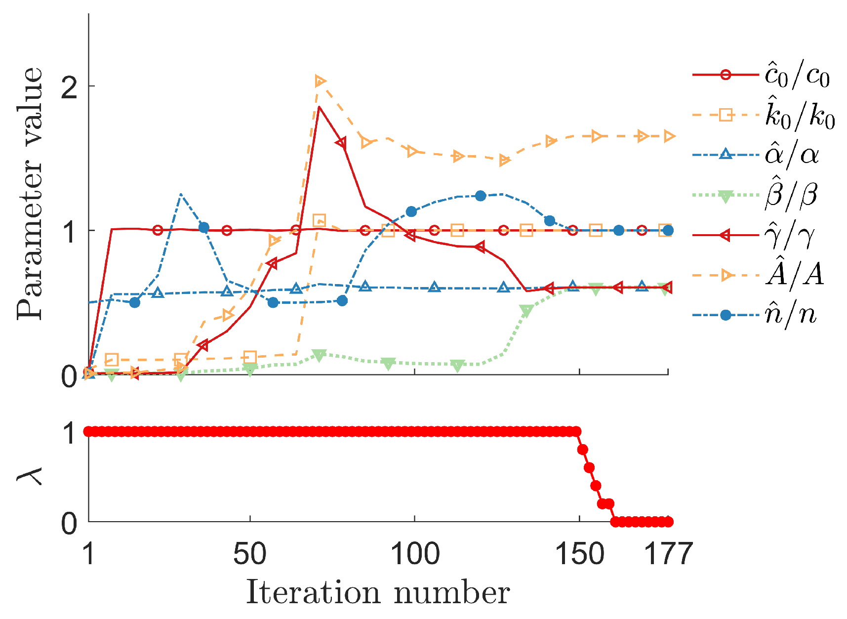
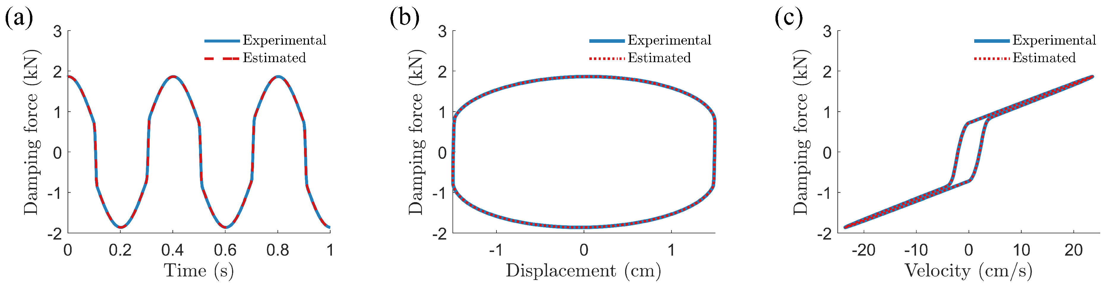
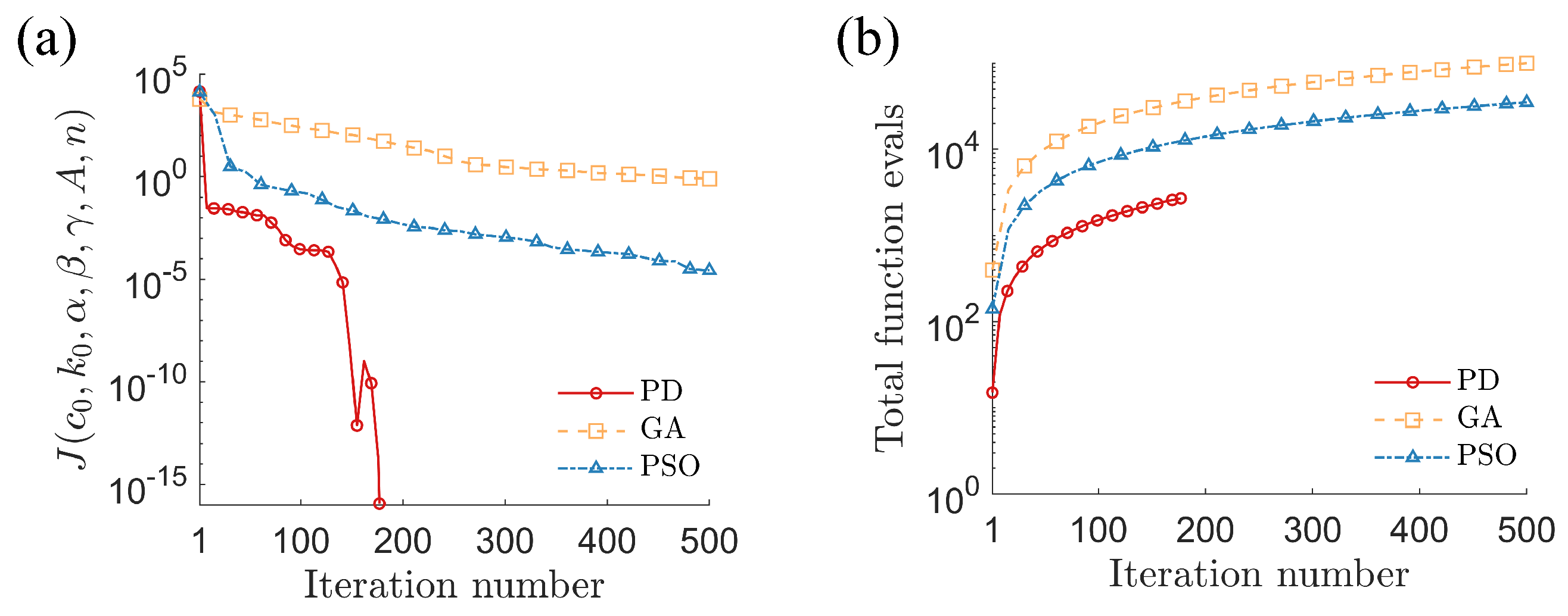
3.3. Magnetorheological Damper System

Magnetorheological (MR) dampers are semi-active devices that use MR fluids to control vibration in structural and mechanical systems [28,29,30]. Adjusting the current delivered to an electromagnet changes its magnetic field, thereby changing the viscosity of the MR fluid. This simple control scheme makes MR dampers ideal for vibration control in vehicle systems [31,32]. MR dampers are also very reliable in practice as they simply act as passive dampers in the event of control system failure. However, for design and implementation in practical applications, one requires a precise mathematical model of the force–displacement behavior of the system. A suitable mathematical model must capture the nonlinear behavior of the system caused by hysteresis.

The Bouc–Wen model is widely used to model the hysteresis behavior of structural and mechanical components [33,34], and is often used to model MR damper systems. In this example, we consider an MR damper system that comprises three parallel force-generating components:

$$F_e\left(t\right)=c_0{\dot{x}}_e\left(t\right)+k_0{x}_e\left(t\right)+\alpha z_e\left(t\right),$$

(18)

where $F_e\left(t\right)$ is the total force applied by the MR damper system, $x_e\left(t\right)$ is the displacement of one end relative to the other (e.g., the relative vertical motion of the sprung and unsprung masses in a vehicle), $c_0$ and $k_0$ are damping and stiffness coefficients, and $\alpha$ represents the ratio between post-elastic stiffness to elastic stiffness of the damper. We do not consider the influence of the applied electrical current on the damping characteristics. The dynamics of the hysteresis component ($z_e\left(t\right)$) are governed by the following differential equation:

$${\dot{z}}_e\left(t\right)=-\gamma \left|{\dot{x}}_e\left(t\right)\right|z_e\left(t\right){\left|z_e\left(t\right)\right|}^{n-1}-\beta {\dot{x}}_e\left(t\right){\left|z_e\left(t\right)\right|}^n+A{\dot{x}}_e\left(t\right).$$

(19)

The parameters $\alpha$, $\beta$, $\gamma$, A, and n determine the hysteresis behavior of the system.

In this example, we identify the system parameters $\mathbf{p}\triangleq \left[c_0,k_0,\alpha ,\beta ,\gamma ,A,n\right]$ assuming the total force ($F_e\left(t\right)$) is measured. The system parameters and bounds are provided in

Table 8. Parameters in the magnetorheological damper system model [35].

Parameter	Units	Experimental Value	Initial Guess	Bounds	Identified Value
$c_0$	N·s·cm$-1$	50	1	$\left[1,400\right]$	$50.00$
$k_0$	N·cm$-1$	25	1	$\left[1,400\right]$	$25.00$
$\alpha$	N·cm$-1$	880	1	$\left[1,1000\right]$	$532.6$
$\beta$	cm$-2$	100	1	$\left[1,400\right]$	$60.52$
$\gamma$	cm$-2$	100	1	$\left[1,400\right]$	$60.52$
A	—	120	1	$\left[1,400\right]$	$198.3$
n	—	2	1	$\left[1,2.5\right]$	$2.000$

. The system is excited by a sinusoidal input displacement of $x_e\left(t\right)=1.5sin\left(5\pi t\right)$, as shown in Figure 8. We use 1-second simulations in this example. To identify the system parameters, we rewrite Equations (18) and (19) in first-order form and add a PD controller:

$$\begin{array}{cc}\hfill F\left(t\right)& ={\widehat{c}}_0{x}_2\left(t\right)+{\widehat{k}}_0{x}_1\left(t\right)+\widehat{\alpha }{x}_3\left(t\right),\hfill \end{array}$$

(20a)

$$\begin{array}{cc}\hfill {\dot{x}}_3\left(t\right)& =-\widehat{\gamma }\left|x_2\left(t\right)\right|x_3\left(t\right){\left|x_3\left(t\right)\right|}^{\widehat{n}-1}-\widehat{\beta }{x}_2\left(t\right){\left|x_3\left(t\right)\right|}^{\widehat{n}}+\widehat{A}{x}_2\left(t\right)+\lambda k_1\left(F_e\left(t\right)-F\left(t\right)\right),\hfill \end{array}$$

(20b)

where $x_1\left(t\right)=1.5sin\left(5\pi t\right)$ and $x_2\left(t\right)$ is its time derivative. In this case, we set gain $k_1=400$ to achieve synchronization when $\lambda =1$ and use the following objective function:

$$J(\widehat{\mathbf{p}},\lambda ,t)={\int }_0^1{\left(F_e\left(t\right)-F(\widehat{\mathbf{p}},\lambda ,t)\right)}^{2}dt.$$

(21)

The initial guess for each parameter (equal to its lower bound) is listed in Table 8.

The evolution of the optimization process using the PD controller is shown in Figure 9; the final identified parameters are listed in the last column of Table 8. Several of the identified parameters differ somewhat from the corresponding experimental values. However, when the identified parameters are used in the original mathematical model (Equations (18) and (19)), the response is in close agreement with the “experimental” response (Figure 10). Thus, the identified parameter values nevertheless produce an accurate overall mathematical model. We again compare the performance of the PD controller with that of GA and PSO strategies [36,37,38], and we again observe that the PD controller obtains a lower objective function value in fewer function evaluations (Figure 11). The comparison between the PD controller and stochastic optimization strategies is summarized in

Table 9. Performance of optimization strategies for the magnetorheological damper system using proportional–derivative controller (PD), genetic algorithm (GA), and particle swarm optimization (PSO) approaches.

Strategy	Number of Iterations	Number of Function Evaluations	Error (J)
PD	177	2716	$1.17\times {10}^{-16}$
GA	500	100,200	$0.804$
PSO	500	35,070	$2.73\times {10}^{-5}$

.

4. Conclusions

In this paper, we have presented a homotopy optimization strategy that uses a proportional–integral–derivative (PID) controller as a penalty function. We have applied this strategy to identify parameters in the van der Pol–Duffing oscillator and two systems of practical importance in engineering applications: a hydraulic engine mount system and a magnetorheological damper system. Through detailed numerical examples, we have demonstrated the utility of the proposed approach to identify model parameters given noisy measurements of only a subset of the system states. We have also compared its performance to that of two popular stochastic optimizers, namely the genetic algorithm and particle swarm optimization strategies. In general, we found the proposed approach to be superior in terms of the solutions that were found as well as the computational effort required. For the hydraulic engine mount system presented in this work, the integral term was found to provide a marginal benefit over a proportional–derivative (PD) controller. We, therefore, recommend considering the PID controller optimization strategy for parameter identification tasks: it is robust, easy to implement, and efficient thanks to its use of a gradient-based optimizer. Future work includes investigating application of the proposed approach to more practical scenarios, such as with data obtained experimentally and approximate mathematical models.

References

1. Gershenfeld, N. The Nature of Mathematical Modeling; Cambridge University Press: Cambridge, MA, USA, 1999. [Google Scholar]
2. Frewin, C. Literature Review and Implementation of Parameter Identification Methods for Multibody Systems Governed by Differential Algebraic Equations; Technical Report; University of Applied Sciences Upper Austria: Wels, Austria, 1 August 2013. [Google Scholar]
3. Söderström, T.; Ljung, L. Theory and Practice of Recursive Identification; MIT Press: Cambridge, MA, USA, 1983. [Google Scholar]
4. Rao, S.S. Engineering Optimization: Theory and Applications; John Wiley & Sons: Hoboken, NJ, USA, 2009. [Google Scholar]
5. Goldberg, D.E. Genetic Algorithms in Search, Optimization and Machine Learning; Addison-Wesley: Boston, MA, USA, 1989. [Google Scholar]
6. Romeijn, H.E.; Smith, R.L. Simulated annealing for constrained global optimization. J. Glob. Optim. 1994, 5, 101–126. [Google Scholar] [CrossRef] [Green Version]
7. Watson, L.T.; Haftka, R.T. Modern homotopy methods in optimization. Comput. Methods Appl. Mech. Eng. 1989, 74, 289–305. [Google Scholar] [CrossRef] [Green Version]
8. Vyasarayani, C.P.; Uchida, T.; McPhee, J. Nonlinear parameter identification in multibody systems using homotopy continuation. J. Comput. Nonlinear Dyn. 2012, 7, 011012. [Google Scholar] [CrossRef] [Green Version]
9. Vyasarayani, C.P.; Uchida, T.; McPhee, J. Single-shooting homotopy method for parameter identification in dynamical systems. Phys. Rev. E 2012, 85, 036201. [Google Scholar] [CrossRef] [PubMed] [Green Version]
10. Luenberger, D.G. Observing the state of a linear system. IEEE Trans. Mil. Electron. 1964, 8, 74–80. [Google Scholar] [CrossRef]
11. Choi, Y.Y.; Kim, S.; Kim, S.; Choi, J.I. Multiple parameter identification using genetic algorithm in vanadium redox flow batteries. J. Power Sources 2020, 450, 227684. [Google Scholar] [CrossRef]
12. Bartkowski, P.; Zalewski, R.; Chodkiewicz, P. Parameter identification of Bouc-Wen model for vacuum packed particles based on genetic algorithm. Arch. Civ. Mech. Eng. 2019, 19, 322–333. [Google Scholar] [CrossRef]
13. Ariza, H.E.; Correcher, A.; Sánchez, C.; Pérez-Navarro, Á.; García, E. Thermal and electrical parameter identification of a proton exchange membrane fuel cell using genetic algorithm. Energies 2018, 11, 2099. [Google Scholar] [CrossRef] [Green Version]
14. Yang, M.; Dai, Y.; Huang, Q.; Mao, X.; Li, L.; Jiang, X.; Peng, Y. A modal parameter identification method of machine tools based on particle swarm optimization. Proc. Inst. Mech. Eng. C J. Mech. Eng. Sci. 2019, 233, 6112–6123. [Google Scholar] [CrossRef]
15. Soon, J.J.; Low, K.S. Photovoltaic model identification using particle swarm optimization with inverse barrier constraint. IEEE Trans. Power Electron. 2012, 27, 3975–3983. [Google Scholar] [CrossRef]
16. Liu, W.; Liu, L.; Chung, I.Y.; Cartes, D.A. Real-time particle swarm optimization based parameter identification applied to permanent magnet synchronous machine. Appl. Soft Comput. 2011, 11, 2556–2564. [Google Scholar] [CrossRef]
17. Abarbanel, H.D.I.; Creveling, D.R.; Farsian, R.; Kostuk, M. Dynamical state and parameter estimation. SIAM J. Appl. Dyn. Syst. 2009, 8, 1341–1381. [Google Scholar] [CrossRef]
18. Cooper, M.; Heidlauf, P.; Sands, T. Controlling chaos—Forced van der Pol equation. Mathematics 2017, 5, 70. [Google Scholar] [CrossRef] [Green Version]
19. Zhihong, Z.; Shaopu, Y. Application of van der Pol–Duffing oscillator in weak signal detection. Comput. Electr. Eng. 2015, 41, 1–8. [Google Scholar] [CrossRef]
20. Ginoux, J.M.; Letellier, C. Van der Pol and the history of relaxation oscillations: Toward the emergence of a concept. Chaos 2012, 22, 023120. [Google Scholar] [CrossRef] [PubMed] [Green Version]
21. Kaplan, B.Z.; Gabay, I.; Sarafian, G.; Sarafian, D. Biological applications of the “filtered” van der Pol oscillator. J. Frankl. Inst. 2008, 345, 226–232. [Google Scholar] [CrossRef]
22. Quaranta, G.; Monti, G.; Marano, G.C. Parameters identification of van der Pol–Duffing oscillators via particle swarm optimization and differential evolution. Mech. Syst. Signal Process. 2010, 24, 2076–2095. [Google Scholar] [CrossRef]
23. Storn, R. On the usage of differential evolution for function optimization. In Proceedings of the 1996 Biennial Conference of the North American Fuzzy Information Processing Society, Berkeley, CA, USA, 19–22 June 1996; pp. 519–523. [Google Scholar]
24. Marzbani, H.; Jazar, R.N.; Fard, M. Hydraulic engine mounts: A survey. J. Vib. Control 2014, 20, 1439–1463. [Google Scholar] [CrossRef]
25. Yu, Y.; Peelamedu, S.M.; Naganathan, N.G.; Dukkipati, R.V. Automotive vehicle engine mounting systems: A survey. J. Dyn. Syst. Meas. Control 2001, 123, 186–194. [Google Scholar] [CrossRef]
26. Flower, W.C. Understanding hydraulic mounts for improved vehicle noise, vibration and ride qualities. SAE Trans. 1985, 94, 832–841. [Google Scholar]
27. Lauß, T.; Oberpeilsteiner, S.; Steiner, W.; Nachbagauer, K. The discrete adjoint method for parameter identification in multibody system dynamics. Multibody Syst. Dyn. 2018, 42, 397–410. [Google Scholar] [CrossRef] [PubMed] [Green Version]
28. Zhu, X.; Jing, X.; Cheng, L. Magnetorheological fluid dampers: A review on structure design and analysis. J. Intell. Mater. Syst. Struct. 2012, 23, 839–873. [Google Scholar] [CrossRef]
29. Bitaraf, M.; Ozbulut, O.E.; Hurlebaus, S.; Barroso, L. Application of semi-active control strategies for seismic protection of buildings with MR dampers. Eng. Struct. 2010, 32, 3040–3047. [Google Scholar] [CrossRef]
30. Dominguez, A.; Sedaghati, R.; Stiharu, I. Modeling and application of MR dampers in semi-adaptive structures. Comput. Struct. 2008, 86, 407–415. [Google Scholar] [CrossRef]
31. Boreiry, M.; Ebrahimi-Nejad, S.; Marzbanrad, J. Sensitivity analysis of chaotic vibrations of a full vehicle model with magnetorheological damper. Chaos Solitons Fractals 2019, 127, 428–442. [Google Scholar] [CrossRef]
32. Yao, G.Z.; Yap, F.F.; Chen, G.; Li, W.H.; Yeo, S.H. MR damper and its application for semi-active control of vehicle suspension system. Mechatronics 2002, 12, 963–973. [Google Scholar] [CrossRef] [Green Version]
33. Bouc, R. Forced vibrations of mechanical systems with hysteresis. In Proceedings of the Fourth Conference on Nonlinear Oscillations, Prague, Czech Republic, 5–9 September 1967; pp. 315–321. [Google Scholar]
34. Wen, Y.K. Equivalent linearization for hysteretic systems under random excitation. J. Appl. Mech. 1980, 47, 150–154. [Google Scholar] [CrossRef]
35. Spencer, B.F., Jr.; Dyke, S.J.; Sain, M.K.; Carlson, J.D. Phenomenological model for magnetorheological dampers. J. Eng. Mech. 1997, 123, 230–238. [Google Scholar] [CrossRef]
36. Xiaomin, X.; Qing, S.; Ling, Z.; Bin, Z. Parameter estimation and its sensitivity analysis of the MR damper hysteresis model using a modified genetic algorithm. J. Intell. Mater. Syst. Struct. 2009, 20, 2089–2100. [Google Scholar] [CrossRef]
37. Kwok, N.M.; Ha, Q.P.; Nguyen, M.T.; Li, J.; Samali, B. Bouc–Wen model parameter identification for a MR fluid damper using computationally efficient GA. ISA Trans. 2007, 46, 167–179. [Google Scholar] [CrossRef]
38. Kwok, N.M.; Ha, Q.P.; Nguyen, T.H.; Li, J.; Samali, B. A novel hysteretic model for magnetorheological fluid dampers and parameter identification using particle swarm optimization. Sens. Actuators A Phys. 2006, 132, 441–451. [Google Scholar] [CrossRef]
Figure 1. Parameter identification problem description for three van der Pol–Duffing oscillators: (ac) single-well, (df) double-well, and (gi) double-hump. (a,d,g): experimental data used for parameter identification ( x 1 e ( t ) ); (b,e,h): shape of objective function over β ( J ( β ) ) for four values of α and with μ = 0.1 ; (c,f,i): basins of attraction with μ = 0.1 . In panels (c,f,i), initial parameter guesses in the dark-red regions lead to local minima when a simple gradient-based optimizer is used; points in the light-green regions lead to the global minimum, indicated with a “target” symbol.
Mathematics 08 01084 g001
Figure 2. Evolution of parameter estimates (normalized relative to experimental values) for three van der Pol–Duffing oscillators: (ac) single-well, (df) double-well, and (gi) double-hump. (a,d,g): parameter identification using proportional–derivative controller; (b,e,h): parameter identification using genetic algorithm; (c,f,i): parameter identification using particle swarm optimization.
Mathematics 08 01084 g002
Figure 3. Error convergence of objective function J ( α , β , μ ) during parameter identification for three van der Pol–Duffing oscillators: (a) single-well, (b) double-well, and (c) double-hump.
Mathematics 08 01084 g003
Figure 4. Computational effort (cumulative number of function evaluations) required to identify parameters for three van der Pol–Duffing oscillators: (a) single-well, (b) double-well, and (c) double-hump.
Mathematics 08 01084 g004
Figure 5. Noisy experimental data (noise-to-signal ratio of 5%) and estimated response using identified parameters for three van der Pol–Duffing oscillators: (a) single-well, (b) double-well, and (c) double-hump.
Mathematics 08 01084 g005
Figure 6. Evolution of parameter estimates (normalized relative to experimental values) for hydraulic engine mount system using five parameter identification strategies: (a) no controller, (b) proportional–derivative controller, (c) proportional–integral–derivative controller, (d) genetic algorithm, and (e) particle swarm optimization.
Mathematics 08 01084 g006
Figure 7. Performance of four strategies to identify parameters for hydraulic engine mount system: (a) error convergence of objective function J ( d H 2 , c E 1 , c E 2 , d E ) ; (b) computational effort required (cumulative number of function evaluations).
Mathematics 08 01084 g007
Figure 8. Input displacement used to identify parameters for the magnetorheological damper system.
Mathematics 08 01084 g008
Figure 9. Evolution of parameter estimates (normalized relative to experimental values) for magnetorheological damper system using proportional–derivative controller.
Mathematics 08 01084 g009
Figure 10. Experimental data and estimated response using identified parameters for magnetorheological damper system: (a) damping force over time, (b) displacement-level hysteretic response, and (c) velocity-level hysteretic response.
Mathematics 08 01084 g010
Figure 11. Performance of three strategies to identify parameters for magnetorheological damper system: (a) error convergence of objective function J ( c 0 , k 0 , α , β , γ , A , n ) ; (b) computational effort required (cumulative number of function evaluations).
Mathematics 08 01084 g011