Resource Exploitation in a Stochastic Horizon under Two Parametric Interpretations

Abstract

This work presents a two-player extraction game where the random terminal times follow (different) heavy-tailed distributions which are not necessarily compactly supported. Besides, we delve into the implications of working with logarithmic utility/terminal payoff functions. To this end, we use standard actuarial results and notation, and state a connection between the so-called actuarial equivalence principle, and the feedback controllers found by means of the Dynamic Programming technique. Our conclusions include a conjecture on the form of the optimal premia for insuring the extraction tasks; and a comparison for the intensities of the extraction for each player under different phases of the lifetimes of their respective machineries.

1. Introduction

In this work we study an extension of the extraction game presented in Reference [1] to the case where the random terminal times follow (different) heavy-tailed distributions which are not necessarily compactly supported. We use the framework of the problem of common non-renewable resource exploitation as was posed in Reference [2], from both—the game-theoretical (cf. Reference [3]) and the actuarial points of view (see References [4,5]).

The first reported works on the dynamic development of exhaustible resources by the members of an oligopoly are those by Hotelling (see References [6,7]). There, we can find the well-known principle of marginal revenue, as well as the standard Hypothesis on the equality between the growth rate and the market interest rate over time. The survey [8] constitutes an excellent introduction to the topic from an Economic point of view, see also Reference [9] for empirical investigation of common-pool resource users’ dynamic and strategic behavior at the micro level using real-world data.

The area owes its main developments to a discussion that took place during the late ‘70s and the early ‘80s on the possibility of replacing the exploitation schemes with some cutting-edge technology to be attained in the near future. The relevance of the debate was the search of a path to move from extracting a non-renewable resource to extracting a renewable one. In this line, we can quote the works of Dasgupta et al. (e.g., References [10,11]; see also Reference [12] Chapter 10.2), and that of Reinganum and Stokey (see Reference [13]). In the former papers, two agents extract a resource that becomes extinct at a time instant which is not known a priori, and then, some technological breakthrough becomes a suitable replacement; while in the latter, the authors assume that the extraction costs equal zero to find an optimal extraction policy over time. From the point of view of our own research, one of the main features of these publications is a method for comparing aggregate extraction paths in terms of the impact of the commitment period of the players on how fast the resource becomes exhausted.

Harris and Vickers [14] revisited Dasgupta’s model, enhanced his analyses on the state dynamics, prove the existence and uniqueness of a Nash equilibrium, and characterize it in terms of the slope of the extraction policies at equilibrium. Epstein [15] and Feliz [16] considered a degenerate game to study the policy of extraction from either one or two wells as the resource dynamics is affected by uncertainty. More recently, the empirical economic knowledge on the subject (along with Hartwick and Solow’s developments—see References [17,18] respectively- on the transformation of an exhaustible resource into productive capital to sustain a steady level of consumption), allowed Van der Ploeg to model the relation between the risk of depletion of a resource with the government policy on debt and precautionary saving (see Reference [19]). In Reference [20], an evolutionary analysis of the renewable resources exploitation with differentiated technologies was undertaken. Comprehensive surveys of models of dynamic games for the development of (renewable and non-renewable) resources can be found in Reference [21] by Van Long, and Reference [12] (Chapter 10) by Dockner et al.

Almost all of the papers mentioned above include the notion of uncertainty. However, only Reference [1] uses random variables to model the terminal times of extraction of the competing firms. We propose a differential game for the extraction of exhaustible resources (see References [12,22] (Chapter 10; Chapter 7)), where we consider uncertainty and asymmetry in a cake-eating model (as shown in Reference [23]), and interpret it in actuarial terms to, for instance, insure the extraction tasks of the players. The uncertainty here is reflected by the fact that the game ends at a random time instant, while the asymmetry can be seen in the different distributions we use for each player involved in the game.

In the insurance literature on non-renewable resource extraction, the work of Stroebel and van Benthem (see Reference [4]) is relevant for our research because they prove that (should the economy is likely to expropriate) the insurance premium on the extraction tasks is increasingly expensive, and decreasingly expensive as the extractors become more expert. Our approach resembles the one used by Delacote (see Reference [24]), because what he sees as households near the extraction points can be, in our case, an agent subjected to a double risk: they will (surely) occupy the place of what we dub Chen extractor (which we prove to be the riskiest of the two players), and they will not be “able to get more than their subsistence requirement” from the wells (the press article [25] presents a narrative of one such situation in Mexico, and the essays in the book [26] delve with the problem in African and Asian countries). There are three more references, in the insurance literature on the extraction of renewable resources, that are important for our developments [27,28,29]. Au lieu of the control methods we adopt, these pieces use statistical methods to show that natural insurance is a normal economic good, and we all agree on the willingness of the agents to pay premia in exchange for a continued supply of the resource under consideration.

The main feature of our game model can be traced back to the works of Petrosyan and Murzov (cf. Reference [30]), and Yaari (cf. Reference [31]). The former used Dynamic Programming to solve a zero-sum pursuit differential game with random duration, while the latter studied the maximization of a utility function by the design of an optimal consumption plan. This topic was further investigated in Reference [32], where the process of technological innovation was supposed to have a random duration. To the best of our knowledge, Petrosyan and Shevkoplyas (Gromova) were the first to propose a general differential game model with random duration (see Reference [33]), including the derivation and solution in closed form under a logarithmic payoff structure, of the corresponding Hamilton-Jacobi-Bellman-Isaacs (HJBI) equations (see Reference [34], and the generalization brought about by Reference [35]).

Game theoretical tools have been applied to model phenomena of the interest of actuarial scientists since the time of the works of Borch and Lemaire, who modelled risk transfers between insurer and reinsurer by means of cooperative games tools (see References [36,37,38]). Among the most relevant and recent works in Actuarial literature related to our work, we can quote Schäl’s paper on the application of stochastic Dynamic Programming for a specific form of the utility function (cf. Reference [5]), because in that research, as well as in ours, we intend to minimize risks in the insurance industry, we focus on a particular form of the reward functions, and we share the use of Dynamic Programming. Such technique is the cornerstone of our approach (the textbook [39] by Hinderer, Rieder and Stieglitz represents an excellent introduction to it, for it covers the deterministic and stochastic cases, and it presents some actuarial applications in insurance). This method has been widely used since its dawn in the decade of the 1960s for many applications, including warfare, resource extraction, and control of pollution in the environment, among others. Schmidli’s textbook [40] presents a complete introduction to the subject with traditional Actuarial Sciences in view. Indeed, he starts with the presentation of stochastic control (by means of Bellman’s principle) in discrete- and continuous-time, then goes to applications in life insurance, and finally presents the classic ruin theory and Merton’s model (Sections 2.6 and 3.1 in the survey [41], and Reference [42] constitute two quick reference guides towards the techniques we use). The works of Dutang et al. (cf. References [43,44]), and that of Polborn (see Reference [45]) present a game theoretic model in discrete-time on a non-life insurance market; and despite the fact that they focus on the competition for the marketshare of the agents, our research can be thought of as a continuation of their model on the fair (optimal) premia to be charged to the agents so as to maximize their profits from the competitive process. Pliska and Ye’s article on optimal life insurance strategies (see Reference [46]), and Mango’s work (cf. Reference [47]) on catastrophe modelling resemble our own contribution, but the characterization of the probability laws that these two works use lies on another extreme of the spectrum of distributions. This is the reason for which the model of perishable inventories with fat-tailed distributions studied by Giri (cf. Reference [48]) is so appealing to us. As for our use of simple contingent functions in association with Markovian processes, the works of Mao and Ostaszewski, and Perry and Stadje on annuity theory (see References [49,50]) represent significant antecedents to our own ideas.

The problem with asymmetry in different random time instants has been studied for some differential games in References [1,51,52,53]. A similar cake-eating problem with different asymmetric discounting functions has been considered in Reference [54]. In our paper we also assume that the game stops at the moment when one of the players quits the extraction tasks. However, rather than a Verhulst-type dynamic for the stock of the resource (see Reference [55]), we use a model that resembles the analysis in Reference [12]. We have chosen to work with the classic two-parameter Weibull distribution and the Chen’s law. Weibull’s model has been widely used in life and non-life Actuarial Mathematics, while Chen’s law owes its importance to the fact that its hazard rate function is –in a broad sense- remarkably stronger than that of the former model; this feature automatically turns it into a very suitable option for modelling extreme events (see Reference [56]). We focus our attention on three phases of the lifetime of the machineries of each player: early stage, normal operation stage, and aging stage. We do this by changing the shape parameters of each one of these laws, for lower value of these parameters ($\delta <1$) results in a lower hazard rate for the distributions; while the choice of $\delta =1$ yields a stable hazard rate function, and a greater value ($\delta >1$) gives us strong failure rates.

Our main conclusions have to do with the implications of using stochastic Dynamic Programming with a particular form of the utility functions, as in Reference [5], however, all of our developments are presented in the continuous-time framework. To this end, we use standard actuarial results and notation, and state a connection between the so-called actuarial equivalence principle (see Chapter 6 in Reference [57], Section on Premium Calculation, Nonlife in References [46,58]), and the feedback controllers found by means of the Dynamic Programming technique. We will end-up showing that, as in References [4,27,28,29], the agents are willing to pay for the coverage of the insurance, in both: the one player context (see References [15,16]), and the game theoretic case with asymmetries (see References [1,51,52,53]); where the unbalance comes from the choice of different fat-tailed distributions for the terminal times of extraction of the agents (see References [50,56,59]).

The rest of the paper is organized as follows. In Section 2 we state the main hypotheses of our model and argue about the connection of the game theoretic framework and the actuarial perspective. Section 3.1 is a reduced version of our study for a degenerate game where only one player performs extraction tasks. This part of the work allows us to exemplify an actuarial interpretation of the verification result given by Theorem 1; and define what we call ease of the extraction of the player in terms of the intensity of the extraction rate. In Section 3.2 we state and explicitly solve the two-player extraction game where the random terminal times are distributed according to Weibull and Chen laws; compare the results in terms of the ease of extraction of each player for particular choices of the parameters; and interpret the verification Theorem 3 in actuarial terms. We give our conclusions in Section 4.

2. Problem Statement

In this section we present the problem we are interested in, introduce our hypotheses, and explain its connection with some ideas from the Actuarial Sciences.

2.1. Game Theoretical Framework

Let us consider the conflict-control process of the extraction of a non-renewable resource in which two participants are involved. We assume that this set of agents remains fixed for the whole duration of the process.

We describe the dynamics of the consumption of the resource by means of the model presented in Reference [12] (Chapter 10.3), according to which,

$$\dot{x}\left(t\right)=-u_1\left(t\right)-u_2\left(t\right),\mathrm{with}x\left(t_0\right)=x_0,$$

(1)

where $x\left(t\right)$ is the amount of the resource available at time $t\ge 0$, $u_i\left(t\right)$ is the extraction rate of the i-th agent at time t, $x_0$ is the initial amount of the stock, and $i=1,2$.

Let $\mathsf{\Gamma }\left(x_0\right)$ be a differential game whose system satisfies the following conditions.

Hypothesis 1. 

(a)Both players act simultaneously and start the game at some initial time $t_0=0$ from the state $x_0$.

(b) 

The control variables of the players are their respective extraction rates at every moment in time, namely $u_1,u_2:[0,\infty )\to \mathcal{U}$, where $\mathcal{U}$ is a compact subset of $[0,\infty )$.

(c) 

The dynamics of the system is given by (1).

The system (1) mirrors the fact that the resource is non-renewable because, by Hypothesis 1(b), $x(·)$ is non-increasing.

We assume that the extraction performed by each agent stops at some random moment of time $T_i$, for $i=1,2$. We impose the following hypothesis on the random terminal times $T_i$.

Hypothesis 2.

The cumulative distribution function of $T_i$ satisfies the following:

(a) 

The random terminal times of the firms are distributed according to some (known) functions $F_i:[0,\infty )\to [0,1]$, $i=1,2$, that satisfy the normalization condition

$${\int }_0^{\infty }\mathrm{d}{F}_i\left(t\right)=1,$$

and that are absolutely continuous with respect to Lebesgue’s measure.

(b) 

Given the different characteristics of the firms, the terminal times of extraction of the same resource are mutually independent.

(c) 

As soon as one of the firms reaches its terminal time, it quits the game and the remaining one keeps extracting the resource until its terminal time is reached (which might happen when the resource becomes extinct).

We define the failure rate function associated with the i-th firm (see References [57,60,61] (Chapter 3; Chapters 4 and 5; Chapter 8.5)) as

$${\lambda }_i\left(t\right):=\frac{f_i\left(t\right)}{1-F_i\left(t\right)},$$

(2)

where $f_i:=F_i^{\prime }$ is a density function for the random terminal time of the i-th player. The existence of such density function is ensured by Hypothesis 2(a).

By virtue of Hypothesis 2(c), $\mathsf{\Gamma }\left(x_0\right)$ collapses to a one-player game at a random terminal time that may be formed by means of the rule of correspondence

$$T:=min\{T_1,T_2\}.$$

(3)

Now, by Hypothesis 2(b), the results in Reference [61] (Chapter 16.3) and the well-known relation

$$1-F_i\left(t\right)=exp\left(-{\int }_0^t{\lambda }_i\left(s\right)\mathrm{d}s\right)$$

(4)

(see Reference [57] (Chapter 3)), we define the distribution function of the random variable T as

$$\begin{array}{cc}\hfill F\left(t\right)& :=1-(1-F_1\left(t\right))(1-F_2\left(t\right))\hfill \\ & =1-{\mathrm{e}}^{-{\int }_{t_0}^t\lambda \left(s\right)\mathrm{d}s},\hfill \end{array}$$

(5)

where $\lambda \left(t\right):={\lambda }_1\left(t\right)+{\lambda }_2\left(t\right)$ stands for the hazard rate function of the random variable T (see, for instance Reference [57] (Chapter 9.3)).

We now introduce the payoff function and the performance indices for each player in the game $\mathsf{\Gamma }\left(x_0\right)$. To do this, we assume the following conditions.

Hypothesis 3.

For $i=1,2$, the utility functions $h_i$ and ${\mathsf{\Phi }}_i$ are continuous in all of their arguments, and concave with respect to $u_i$. Additionally, the function $h_i$ satisfies either:

(a) 

It is a nonnegative function, that is: $h_i:\mathbb{R}\times {\mathcal{U}}^n\to [0,\infty )$.

(a’) 

The product $f_i·h_i$ is such that

$${\int }_0^{\infty }{\int }_0^{\infty }|f_i\left(t\right)·h_i(x\left(\tau \right),u_1\left(\tau \right),u_2\left(\tau \right))|\mathrm{d}t\mathrm{d}\tau <\infty .$$

At time T given by (3), if the i-th player is the only one remaining in the extraction game, she receives a terminal payoff ${\mathsf{\Phi }}_i\left(x\left(T\right)\right)$.

With Hypothesis 3, we can introduce the performance index we are interested in.

Define $u:[0,\infty )\to {\mathcal{U}}^2$ as the vector of functions $(u_1,u_2)$. For $i=1,2$, the performance index for the i-th player is:

$$\begin{array}{ccc}\hfill K_i(x_0,u_1,u_2)& =& {\mathbb{E}}_{x_0}^{u_1,u_2}\left[{\int }_0^{T_i}{h}_i(x\left(\tau \right),u_1\left(\tau \right),u_2\left(\tau \right))\mathrm{d}\tau {\chi }_{\{T_i\le T_j\}}\right]\hfill \end{array}$$

(6)

$$\begin{array}{cc}\hfill & +{\mathbb{E}}_{x_0}^{u_1,u_2}\left[{\int }_0^{T_j}{h}_i(x\left(\tau \right),u_1\left(\tau \right),u_2\left(\tau \right))\mathrm{d}\tau {\chi }_{\{T_i>T_j\}}\right]\hfill \end{array}$$

(7)

$$\begin{array}{cc}\hfill & +{\mathbb{E}}_{x_0}^{u_1,u_2}\left[{\mathsf{\Phi }}_i\left(x\left(T\right)\right){\chi }_{\{T_i>T_j\}}\right],\hfill \end{array}$$

(8)

where ${\mathbb{E}}_{x_0}^{u_1,u_2}[·]$ is the conditional expectation of · given that the initial stock is $x_0$, and the agents use the strategies $u_1$ and $u_2$; ${\chi }_{\{·\}}$ is an indicator function; T is as in (3); and ${\mathsf{\Phi }}_i(·)$ is the terminal payoff function referred to in the final part of Hypothesis 3.

Remark 1.

Note that the payoff of the game has two components: the integral payoff (6) and (7); achieved while playing, and (8), a final reward, which is assigned to the player that stayed longer in the system.

Now we use the compactness mentioned in Hypothesis 1(b) to introduce the sort of optimality we are interested in.

Definition 1.

Let ${\Pi }^i:=\{u_i:[0,\infty )\times [0,x_0]\to [0,x_0]|u_i\mathit{is}\mathit{Lebesgue-measurable}\},$ for $i=1,2$. We say that a pair of feedback strategies $(u_1^{*},u_2^{*})\in {\Pi }^1\times {\Pi }^2$ is optimal if it is a so-called Nash equilibrium, that is, if

$$\begin{array}{ccc}\hfill K_1(x_0,u_1^{*},u_2^{*})& \ge & K_1(x_0,u_1,u_2^{*})\mathit{for}\mathit{every}{u}_1\in {\Pi }^1,\hfill \\ \hfill K_2(x_0,u_1^{*},u_2^{*})& \ge & K_2(x_0,u_1^{*},u_2)\mathit{for}\mathit{every}{u}_2\in {\Pi }^2.\hfill \end{array}$$

In this game, each firm intends to maximize its profit. Then, we designate the corresponding strategies of the players as $u_1^{*},u_2^{*}$, and call them “optimal”. We also write the trajectory under such strategies as $x^{*}$, and also call it “optimal trajectory”. Let $h_i^{*}\left(t\right):=h_i(x^{*},u_1^{*},u_2^{*})$, and rewrite the optimal expected payoff resulting from the maximization of (6)–(8) as

$$\begin{array}{ccc}\hfill K_i(x_0,u_1^{*},u_2^{*})& \hfill =& {\mathbb{E}}_{x_0}^{u_1^{*},u_2^{*}}\left[{\int }_0^{T_i}{h}_i^{*}\left(\tau \right)\mathrm{d}\tau {\chi }_{\{T_i\le T_j\}}\right]\hfill \\ \hfill & \hfill & +{\mathbb{E}}_{x_0}^{u_1^{*},u_2^{*}}\left[{\int }_0^{T_j}{h}_i^{*}\left(\tau \right)\mathrm{d}\tau {\chi }_{\{T_i>T_j\}}\right]\hfill \\ \hfill & \hfill & +{\mathbb{E}}_{x_0}^{u_1^{*},u_2^{*}}\left[{\mathsf{\Phi }}_i\left(x^{*}\left(T\right)\right){\chi }_{\{T_i>T_j\}}\right].\hfill \end{array}$$

The following result is an extension of Reference [1] (Corollary 3.1). We include its proof here for the sake of completeness.

Proposition 1.

Let Hypotheses 1–3 hold. If

$$H_i\left(\theta \right):={\int }_0^{\theta }{h}_i^{*}\left(t\right)\mathrm{d}t<\infty$$

(9)

for all $\theta >0$, then the optimal expected payoff for the problem starting at $t=0$ is given by

$$K_i(x_0,u_1^{*},u_2^{*})={\int }_0^{\infty }{h}_i^{*}\left(\theta \right)(1-F\left(\theta \right))+{\mathsf{\Phi }}_i\left(x^{*}\left(\theta \right)\right)f_j\left(\theta \right)(1-F_i\left(\theta \right))\mathrm{d}\theta .$$

Proof. 

It is easy to see that

$$\begin{array}{ccc}\hfill K_i(x_0,u_1^{*},u_2^{*})& =& {\int }_0^{\infty }{\int }_0^{\infty }{\int }_0^{\theta }{h}_i^{*}\left(t\right)\mathrm{d}t{\chi }_{\{\theta <\tau \}}{f}_j\left(\tau \right)\mathrm{d}\tau f_i\left(\theta \right)\mathrm{d}\theta \hfill \\ & & +{\int }_0^{\infty }{\int }_0^{\infty }{\int }_0^{\tau }{h}_i^{*}\left(t\right)\mathrm{d}t{\chi }_{\{\theta >\tau \}}{f}_i\left(\theta \right)\mathrm{d}\theta f_j\left(\tau \right)\mathrm{d}\tau \hfill \\ & & +{\int }_0^{\infty }{\int }_0^{\infty }{\mathsf{\Phi }}_i\left(x^{*}\left(\tau \right)\right){\chi }_{\{\theta >\tau \}}{f}_j\left(\tau \right)\mathrm{d}\tau f_i\left(\theta \right)\mathrm{d}\theta .\hfill \end{array}$$

The use of (9) and Fubini’s rule yield

$$\begin{array}{ccc}\hfill K_i(x_0,u_1^{*},u_2^{*})& =& {\int }_0^{\infty }{\int }_0^{\tau }{H}_i\left(\theta \right)f_i\left(\theta \right)\mathrm{d}\theta f_j\left(\tau \right)\mathrm{d}\tau +{\int }_0^{\infty }{\int }_0^{\theta }{H}_i\left(\tau \right)f_j\left(\tau \right)\mathrm{d}\tau f_i\left(\theta \right)\mathrm{d}\theta \hfill \end{array}$$

(10)

$$\begin{array}{c}+{\int }_0^{\infty }{\int }_0^{\infty }{\mathsf{\Phi }}_i\left(x^{*}\left(\tau \right)\right){\chi }_{\{\theta >\tau \}}{f}_j\left(\tau \right)\mathrm{d}\tau f_i\left(\theta \right)\mathrm{d}\theta .\hfill \end{array}$$

(11)

An integration by parts yields

$$\begin{array}{cc}\hfill & {\int }_0^{\infty }{\int }_0^{\tau }{H}_i\left(\theta \right)f_i\left(\theta \right)\mathrm{d}\theta f_j\left(\tau \right)\mathrm{d}\tau +{\int }_0^{\infty }{\int }_0^{\theta }{H}_i\left(\tau \right)f_j\left(\tau \right)\mathrm{d}\tau f_i\left(\theta \right)\mathrm{d}\theta \hfill \end{array}$$

(12)

$$\begin{array}{c}= {\int }_0^{\infty }{H}_i\left(\theta \right)f_i\left(\theta \right)\mathrm{d}\theta -{\int }_0^{\infty }{H}_i\left(\theta \right)f_i\left(\theta \right)F_j\left(\theta \right)\mathrm{d}\theta \hfill \end{array}$$

(13)

$$\begin{array}{c}+{\int }_0^{\infty }{H}_i\left(\theta \right)f_j\left(\theta \right)\mathrm{d}\theta -{\int }_0^{\infty }{H}_i\left(\theta \right)f_j\left(\theta \right)F_i\left(\theta \right)\mathrm{d}\theta .\hfill \end{array}$$

(14)

Working with ${\int }_0^{\infty }{H}_i\left(\theta \right)f_i\left(\theta \right)\mathrm{d}\theta$ and ${\int }_0^{\infty }{H}_i\left(\theta \right)f_i\left(\theta \right)F_j\left(\theta \right)\mathrm{d}\theta$ separately yields:

$$\begin{array}{ccc}\hfill {\int }_0^{\infty }{H}_i\left(\theta \right)f_i\left(\theta \right)\mathrm{d}\theta & =& \underset{\theta \to \infty }{lim}{H}_i\left(\theta \right)-{\int }_0^{\infty }{h}_i^{*}\left(\theta \right)F_i\left(\theta \right)\mathrm{d}\theta ,\hfill \\ \hfill {\int }_0^{\infty }{H}_i\left(\theta \right)f_i\left(\theta \right)F_j\left(\theta \right)\mathrm{d}\theta & =& \underset{\theta \to \infty }{lim}{H}_i\left(\theta \right)-{\int }_0^{\infty }{H}_i\left(\theta \right)f_j\left(\theta \right)F_i\left(\theta \right)\mathrm{d}\theta -{\int }_0^{\infty }{h}_i^{*}\left(\theta \right)F_i\left(\theta \right)F_j\left(\theta \right)\mathrm{d}\theta .\hfill \end{array}$$

(15)

The last relations imply

$${\int }_0^{\infty }{H}_i\left(\theta \right)f_i\left(\theta \right)F_j\left(\theta \right)\mathrm{d}\theta +{\int }_0^{\infty }{H}_i\left(\theta \right)f_j\left(\theta \right)F_i\left(\theta \right)\mathrm{d}\theta =\underset{\theta \to \infty }{lim}{H}_i\left(\theta \right)-{\int }_0^{\infty }{h}_i^{*}\left(\theta \right)F_i\left(\theta \right)F_j\left(\theta \right)\mathrm{d}\theta .$$

(16)

Substituting (15) and (16) in (12)–(14) and collecting similar terms yield:

$$\begin{array}{cc}& {\int }_0^{\infty }{\int }_0^{\tau }{H}_i\left(\theta \right)f_i\left(\theta \right)\mathrm{d}\theta f_j\left(\tau \right)\mathrm{d}\tau +{\int }_0^{\infty }{\int }_0^{\theta }{H}_i\left(\tau \right)f_j\left(\tau \right)\mathrm{d}\tau f_i\left(\theta \right)\mathrm{d}\theta \hfill \\ =& \underset{\theta \to \infty }{lim}{H}_i\left(\theta \right)-{\int }_0^{\infty }{h}_i^{*}\left(\theta \right)\left(F_i\left(\theta \right)+F_j\left(\theta \right)-F_i\left(\theta \right)F_j\left(\theta \right)\right)\mathrm{d}\theta \hfill \\ =& {\int }_0^{\infty }{h}_i^{*}\left(\theta \right)\left(1-F\left(\theta \right)\right)\mathrm{d}\theta .\hfill \end{array}$$

(17)

Note that the term ${\int }_0^{\infty }{\int }_0^{\infty }{\mathsf{\Phi }}_i\left(x^{*}\left(\tau \right)\right){\chi }_{\{\theta >\tau \}}{f}_j\left(\tau \right)\mathrm{d}\tau f_i\left(\theta \right)\mathrm{d}\theta$ in (11) equals

$$\begin{array}{ccc}\hfill {\int }_0^{\infty }{\mathsf{\Phi }}_i\left(x^{*}\left(\tau \right)\right)f_j\left(\tau \right)\mathrm{d}\tau f_i\left(\theta \right)\mathrm{d}\theta & =& {\int }_0^{\infty }{\mathsf{\Phi }}_i\left(x^{*}\left(\theta \right)\right)f_j\left(\theta \right)\mathrm{d}\theta -{\int }_0^{\infty }{F}_i\left(\theta \right){\mathsf{\Phi }}_i\left(x^{*}\left(\theta \right)\right)f_j\left(\theta \right)\mathrm{d}\theta \hfill \\ & =& {\int }_0^{\infty }{\mathsf{\Phi }}_i\left(x^{*}\left(\theta \right)\right)f_j\left(\theta \right)\left(1-F_i\left(\theta \right)\right)\mathrm{d}\theta ,\hfill \end{array}$$

(18)

where the first equality is due to an integration by parts. The substitution of (17) and (18) in (10) and (11) gives the result. □

2.2. Interconnection with the Actuarial Sciences

In the traditional Actuarial Sciences literature, there are two main principles under which it is possible to compute the amount (of money, time or effort) to be invested/reserved –know as “premium” (premia)- in exchange for a benefit (e.g., the coverage of an insurance or the earnings of the extraction tasks). These principles are classified according to the following methodologies.

PI. 

Optimization of the probability that the trajectory $x(·)$ attains certain set. This approach and its refinements yield what is called “percentile premium”, “value-at-risk” (see References [60,62] (Chapters 3.5.3 and 3.5.4)) or “risk premium” (see Reference [61] (Example 6.5 and Chapter 17)).

PII. 

Search of a premium such that the decision maker is indifferent between taking the risk or not. This is typically done by setting the expectation of the utility function under uncertainty equal to the utility function without risk. A remarkable simplification arises when the utility function is linear, for in that case, the expectation of the prospective loss turns out to be null, and the computation of the corresponding surcharge is very straightforward (see Reference [57] (Example 6.1.1)). The result of this method is called “equivalence premium”, “indifferent price”, or “utility/benefit premium”.

From the point of view of the actuarial scientist, we are using a third principle, which connects the traditional approaches. Thus, we state such third principle:

PIII. 

Optimization of the conditional expectation (6)–(8) (see References [40] and [63] (Chapter 6)) to find the premium which is to be exchanged for the benefits derived from the extraction tasks. Such a mixture resembles the approach of the tail-value-at-risk –also dubbed conditional tail expectation and expected shortfall- (cf. References [64,65,66] and [60] (Chapter 3.5.4)) from PI, in the sense that the objective function of the optimization program we work with is a conditional expectation. However, due to the logarithmic form of the reward functions we use; and the particular form of the HJBI equations that this yields, the premia we obtain are very much alike the indifferent prices one would get, should one have chosen to work with the equivalence principle from PII in the first place (see the Remarks 2 and 3 below). In the present context, we follow References [31,33] to present the development of the extraction tasks as a process with uncertain duration, and interpret the maximizers $u_1^{*}$ and $u_2^{*}$ as measures of the value’s cost that each of the agents earns from such development, that is, as the premia that they should invest in order to ensure/insure their operation.

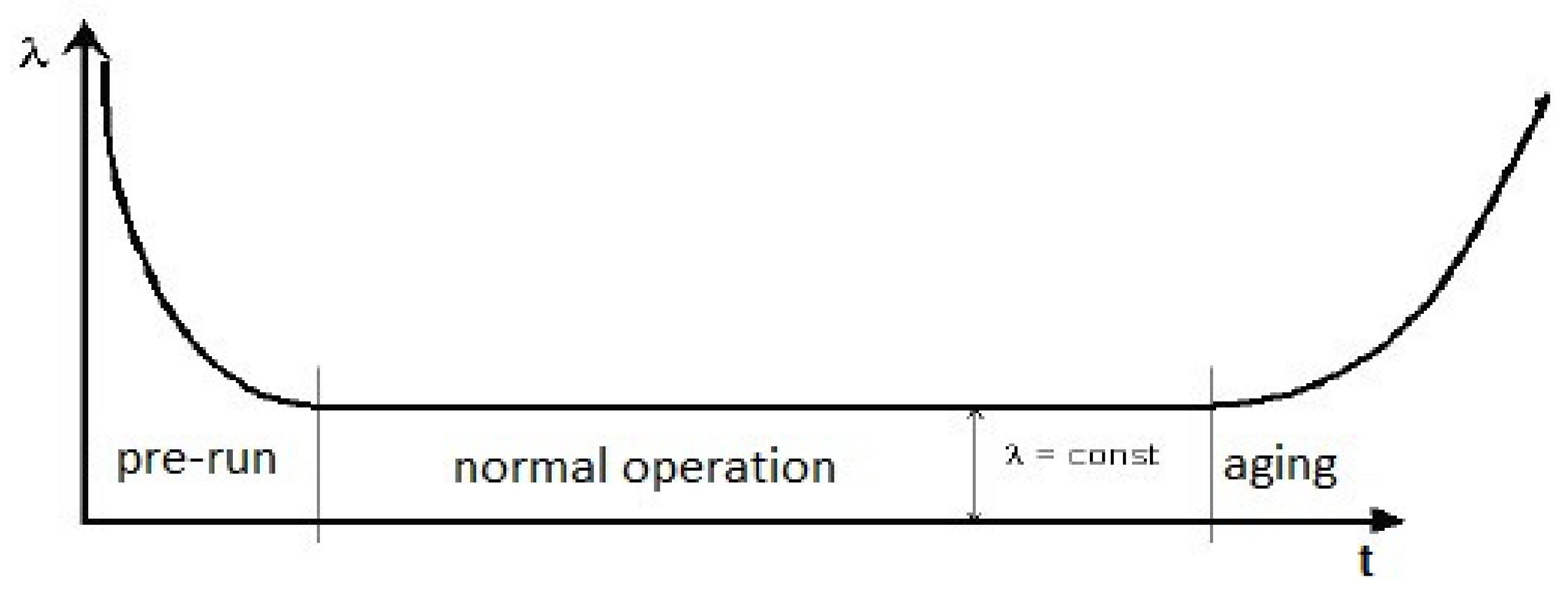
We consider games with a random terminal time T, to which the basic terminology of reliability theory can be applied directly. In fact, the failure rate function (2) can be thought of as a conditional density provided that the agent did not default (i.e., leave the game until the moment t). In our terminology, we would talk about the density of the terminal time of the game, provided that the game was not terminated before the moment t. The failure rate function ${\lambda }_i\left(t\right)$ that describes the life cycle for the player i has the form described by Figure 1. We follow Reference [67] (Chapter 1) to identify three phases of the hazard rate with respect to time.

• The first phase is called the pre-run phase. According to the theory of reliability, the failures in this phase arise due to undetectable latent defects. Specificity of this problem is understandable not only from the point of view of the application of elements to technical systems, in actuarial risk theory, for such a period the terms “newborn period”, “infant mortality” and “early failures” can be used (see Reference [57] (Chapter 3)). From the point of view of game theory, early failures can be caused by inexperience, that is, inconsistency of the players just who just entered the game. The failure rate function ${\lambda }_i(·)$ in this phase is a decreasing function of time.
• The next period of the life cycle of the system is the so-called period of normal system operation. The failure rate function ${\lambda }_i(·)$ in this period is constant (or approximately constant), and the sudden failures themselves are caused by imperfection of the system itself, or are caused by some external factor. This is called the “adult” period of the process (see Reference [67] (Chapters 1, 3 and 5)). The game in the period under consideration can stop under the influence of some unforeseen circumstances of the external environment.
• In the last period, the system goes into the aging phase. The system failures in this period are associated with how the system ages, and that’s why the failure rate function $\lambda \left(t\right)$ is an increasing function.

Moreover, we are interested in presenting a comparative analysis of the results when the duration of the extraction is distributed according to the laws of Weibull and Chen. The former has been widely used for modelling losses, time-until-failure of many non-renewable electronic devices (electronic lamps, semiconductor devices, some microwave devices) and lifetimes in general (see References [57,59,60,61,67]), while the latter is a fat-tailed distribution (see Reference [56]).

The cumulative distribution function of the Weibull distribution is:

$$F_1\left(t\right)=1-exp\left(-{\lambda }_1{t}^{{\delta }_1}\right),$$

(19)

where ${\lambda }_1>0$ is a scale parameter, and ${\delta }_1>0$ is a shape parameter that corresponds to one of the three phases in which the lifetime of the player can be located. Namely, the value ${\delta }_1<1$ corresponds to the pre-run period, here the failure rate function ${\lambda }_1\left(t\right)$ is a decreasing function of t. At ${\delta }_1=1$, the system is in the normal operation mode, and ${\lambda }_1(·)$ equals a constant value of ${\lambda }_1>0$. We note that for ${\delta }_1=1$, the Weibull distribution corresponds to an exponential distribution. For ${\delta }_1>1$, the system is in an aging state, therefore ${\lambda }_1(·)$ is an increasing function. A special case of the Weibull distribution for this instance is the so-called Rayleigh distribution (see Reference [60] (Appendix A.3)). We are in this case when ${\delta }_1=2$.

By (2), the corresponding failure rate function is

$${\lambda }_1\left(t\right)={\lambda }_1{\delta }_1{t}^{{\delta }_1-1}.$$

(20)

The cumulative distribution function of Chen distribution is

$$F_2\left(t\right)=1-exp\left({\lambda }_2\left(1-{\mathrm{e}}^{t^{{\delta }_2}}\right)\right),$$

(21)

where ${\lambda }_2>0$ is a scale parameter, and ${\delta }_2>0$ is a shape parameter. Now, for this case, it follows from (2) that the failure rate function takes the form

$${\lambda }_2\left(t\right)={\lambda }_2{\delta }_2{t}^{{\delta }_2-1}{\mathrm{e}}^{t^{{\delta }_2}}.$$

(22)

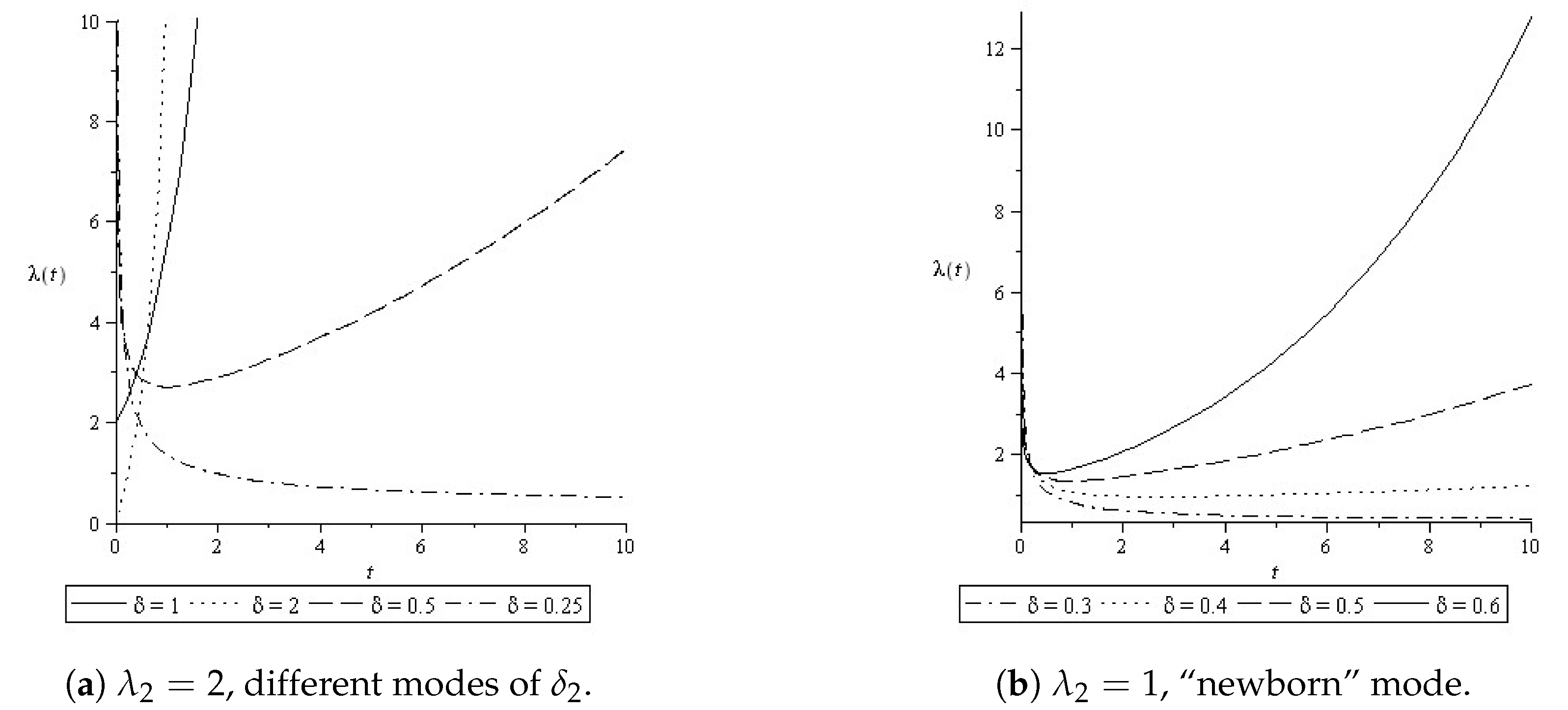
If ${\delta }_2<1$, we will be at the “newborn” phase. Here, the failure rate function ${\lambda }_2(·)$ is bathtub-shaped. This corresponds to a realistic process of extracting natural resources. When ${\delta }_2=1$, the system is in the normal operation mode and the hazard rate function ${\lambda }_2(·)$ is increasing. At ${\delta }_2>1$, the system is in aging state, and ${\lambda }_2(·)$ is also an increasing function, but from

$${\lambda }_2^{\prime }\left(t\right)={\lambda }_2{\delta }_2{t}^{{\delta }_2-1}{\mathrm{e}}^{t^{{\delta }_2}}{for}t>0,$$

it is straightforward that the growth rate of ${\lambda }_2(·)$ is noticeably larger than in the case of normal operation. This implies that there is a greater probability of failure at this stage of the extraction.

Graphical representations of the failure rate function of Chen distribution for two values of the scale parameter ${\lambda }_2$ are shown in Figure 2. In Figure 2b, note that, as $\delta \to 1$, the slope of the graph grows larger. This fact might be interpreted by arguing that Chen’s distribution plausibly describes how the system goes from the pre-run state into the normal operation mode.

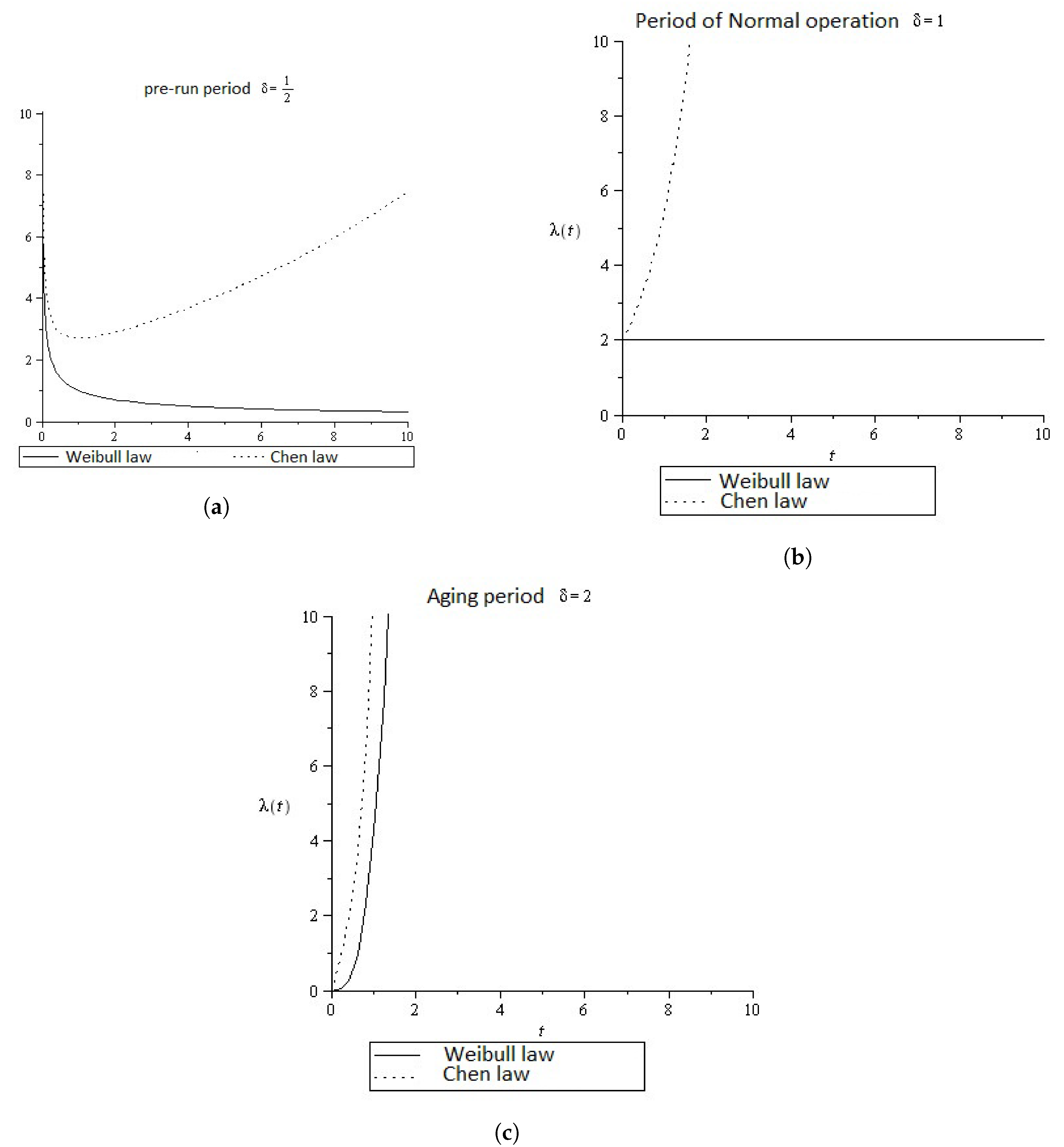
Graphical representations of the failure rate functions for the Weibull and Chen distributions for fixed ${\lambda }_1=2={\lambda }_2$, and the same values of the parameter ${\delta }_1$ and ${\delta }_2$ are shown in Figure 3. Note that we display these functions for each of the periods we have identified.

3. Resource Exploitation under Two Parametric Interpretations

It is easy to see that Weibull and Chen distributions (19) and (21) verify the Hypothesis 2(a). We will consider the cases of these probability laws for the random terminal times of the players, and take $T=min\{T_1,T_2\}$ for different parameters of these families. This will allow us to model failures of the equipments depending on their operation mode.

3.1. Dynamic Models for the Extraction of Natural Resources by One Agent

In this section, we follow Reference [32], and consider the situation where only one agent performs extraction tasks, that is, the degenerate game where $n=1$ (in this case, we do not consider a terminal payoff function, because the game finishes as soon as the only player leaves the system). Let $x\left(t\right)$ be the stock of the non-renewable resource under consideration. Then, the dynamics (1) reduces to

$$\dot{x}\left(t\right)=-u\left(t\right),x\left(t_0\right)=x_0>0,$$

(23)

where $u\left(t\right)\ge 0$. An application of Proposition 1 yields that the expected payoff of the agent, provided that the terminal random time follows Weibull’s law, that is

$$K(x_0,u)={\int }_0^{\infty }h(x\left(t\right),u\left(t\right)){\mathrm{e}}^{-\lambda t^{\delta }}\mathrm{d}t.$$

(24)

Note that adding a terminal cost does not make sense with a single agent, so we set $\mathsf{\Phi }\left(x\right)\equiv 0$.

If we use Chen’s law for the random terminal time, the winnings of the extractor are given by

$$K(x_0,u)={\int }_0^{\infty }h(x\left(t\right),u\left(t\right))exp\left[-\lambda \left(1-{\mathrm{e}}^{t^{\delta }}\right)\right]\mathrm{d}t.$$

(25)

The problem of obtaining feedback maximizers for the expected gains in Formulae (24) and (25) under the condition (23) can be solved using the following Bellman equation

$$\begin{array}{c}\hfill \lambda \left(t\right)W(x,t)=\frac{\partial }{\partial t}W(x,t)+\underset{u}{max}\left(h(t,u)-u\frac{\partial }{\partial x}W(x,t)\right),\end{array}$$

(26)

with transversality condition

$$\underset{t\to \infty }{lim}W(x,t)=0.$$

(27)

In (26), $\lambda (·)$ corresponds either to the failure rate of Weibull or Chen distributions. The details on the necessary calculations for achieving (26) and (27) can be seen in, for instance Reference [68] (Chapter I.5).

The following result assumes a specific form of the agent’s utility function. There are, of course, many other forms, which need to be concave, continuous and non-decreasing. However, we have chosen this particular form because of the interest that the result has from the point of view of the Actuarial Scientist (see Remark 2 below).

Theorem 1.

If the utility function is of the form

$$h(x,u)=lnu,$$

(28)

then the optimal controller is given by the Lebesgue-measurable function

$$u^{*}(t,x)=\frac{x}{{\overline{a}}_t},$$

(29)

where

$${\overline{a}}_t:={\int }_0^{\infty }\frac{1-F(t+s)}{1-F\left(t\right)}\mathrm{d}s.$$

(30)

Proof. 

The substitution of the ansatz (see References [34,35]):

$$W(x,t)=A\left(t\right)lnx+B\left(t\right),$$

(31)

into Bellman’s Equation (26) yields

$$\begin{array}{ccc}\hfill \frac{\partial }{\partial x}W(x,t)& =& \frac{A\left(t\right)}{x},\hfill \end{array}$$

(32)

$$\begin{array}{ccc}\hfill \frac{\partial }{\partial t}W(x,t)& =& \dot{A}\left(t\right)lnx+\dot{B}\left(t\right).\hfill \end{array}$$

(33)

Plugging (32) and (33) into (26) gives us that the maximized control is:

$$u^{*}(t,x)=\frac{x}{A\left(t\right)},$$

(34)

and also the following system of differential equations:

$$\begin{array}{ccc}\hfill \dot{A}\left(t\right)-\lambda \left(t\right)A\left(t\right)+1& =& 0;\hfill \end{array}$$

(35)

$$\begin{array}{ccc}\hfill \dot{B}\left(t\right)-\lambda \left(t\right)B\left(t\right)-ln\left(A\left(t\right)\right)-1& =& 0.\hfill \end{array}$$

(36)

The transversality condition (27) takes the form

$$\begin{array}{ccc}\hfill \underset{t\to \infty }{lim}A\left(t\right)& =& 0,\hfill \end{array}$$

(37)

$$\begin{array}{ccc}\hfill \underset{t\to \infty }{lim}B\left(t\right)& =& 0.\hfill \end{array}$$

(38)

Using (37) and (thus) the integrating factor (4) we can solve (35) and get

$$\begin{array}{ccc}\hfill A\left(t\right)& =& \frac{1}{1-F\left(t\right)}{\int }_t^{\infty }{\mathrm{e}}^{-{\int }_0^s\lambda \left(\tau \right)\mathrm{d}\tau }\mathrm{d}s\hfill \\ & =& \frac{{\int }_t^{\infty }1-F\left(s\right)\mathrm{d}s}{1-F\left(t\right)}.\hfill \end{array}$$

The last equality follows from (4). Here, of course, $F(·)$ is given by (19) or (21).

From (30), it is straightforward that

$$A\left(t\right)={\overline{a}}_t.$$

(39)

The substitution of (39) in (34) gives (29).

The fact that the controller (29) is optimal for the degenerate game follows from Theorem I.7.1(a) in Reference [68]. The fact that that such controller is Lebesgue-measurable follows from Hypothesis 1(b), along with the so-named measurable selection theorems (see, for instance, References [69,70,71] (Theorem 12.1; Proposition D5(a); Theorem 3.4)). This proves the result. □

Remark 2.

An actuarial interpretation of Theorem 1 is the fact that the function $A\left(t\right)$ agrees with the expectation of the so-called contingent life annuity with $0\%$ interest rate for a life aged $\left(t\right)$ displayed in (30) (see Reference [57] (Chapter 5.2)) and write

$$x-u^{*}(t,x)·{\overline{a}}_t=0.$$

(40)

This expression is remarkably similar to the relations (6.2.3)–(6.2.4) in Reference [57] (see PII in Section 2.2, References [57,58] (Chapters 6.2 and 7.2; sections on Premium Calculation for Nonlife Insurance), which are used to establish the equivalence premium $u^{*}(t,x)$ that is to be continuously paid to obtain a benefit of x. In the Actuarial Mathematics literature, we use this expression to state the existence of a balance between an expected income $u^{*}(t,x)·{\overline{a}}_t$ (that will be paid over a contingent horizon), and an expected benefit x (that will be received at a given moment of time). From this point of view, we might distinguish two parts within the Lebesgue-measurable optimal rate of extraction $u^{*}(t,x)$ from (29):

(i) 

the benefit that the agent will eventually get, x; and

(ii) 

the intensity of the extraction that the agent needs to apply to acquire $u^{*}(t,x)$, that is, $A\left(t\right)={\overline{a}}_t$.

Keeping this in mind, we can state that the resulting instantaneous utility of obtaining x by continuously extracting $u^{*}(t,x)$ with an intensity of ${\overline{a}}_t$ is given by $h(x,u)$ in (28).

Since the intensity of the extraction appears in the denominator of (29), we will dub $\frac{1}{{\overline{a}}_t}$ as ease of extraction. Our goal is to emphasize the inverse proportionality of the optimal controller $u^{*}(t,x)$ with respect to the intensity of extraction ${\overline{a}}_t$.

We obtain the following result as a by-product of Theorem 1.

Theorem 2.

If the utility function is of the form (28), then the value function for the optimal control problem of maximizing (6) within $\mathcal{U}$ subject to (1) is given by

$$W(x,t)={\overline{a}}_{t}lnx+{\int }_0^{\infty }(1+ln{\overline{a}}_s)\frac{1-F(s+t)}{1-F\left(t\right)}\mathrm{d}s.$$

(41)

Proof. 

From (31), we readily know that

$$W(x,t)={\overline{a}}_{t}lnx+B\left(t\right).$$

To find the function $B\left(t\right)$, we note that the transversality condition (38) and again, the integrating factor (4) give that

$$\begin{array}{ccc}\hfill B\left(t\right)& =& \frac{{\int }_t^{\infty }exp\left(-{\int }_0^s\lambda \left(\tau \right)\mathrm{d}\tau \right)\left(1+lnA\left(s\right)\right)\mathrm{d}s}{exp\left(-{\int }_0^t\lambda \left(s\right)\mathrm{d}s\right)}\hfill \\ & =& \frac{{\int }_t^{\infty }\left(1-F\left(s\right)\right)\left(1+ln{\overline{a}}_s\right)\mathrm{d}s}{1-F\left(t\right)}.\hfill \end{array}$$

(42)

The last equality follows from (4) and (39). Substituting (42) into (31) gives (41). The fact that this function is actually the value of the optimal control problem of maximizing (6) subject to (1) follows from the verification Theorem I.7.1(b) in Reference [68]. This proves the result. □

3.1.1. Normal Mode (${\delta }_1=1={\delta }_2$)

As we already stated, for the case of Weibull distribution, when ${\delta }_1=1$, the random terminal time is exponentially distributed with mean ${\lambda }_1^{-1}$. Then, by Theorem 1, the optimal strategy of the agent is $u^{*}(t,x)={\lambda }_{1}x$. We solve (23) and get that the optimal trajectory is

$$x^{*}\left(\tau \right)=x_0{\mathrm{e}}^{-{\lambda }_1\tau }.$$

For the case of Chen’s law, we let ${\delta }_2=1$ and substitute (22) into (29) to get

$$u^{*}(t,x)=\frac{xexp\left(-{\lambda }_2{\mathrm{e}}^t\right)}{{\int }_t^{\infty }exp\left(-{\lambda }_2{\mathrm{e}}^s\right)\mathrm{d}s}.$$

We substitute this controller into (23) and solve the differential equation to obtain the optimal trajectory when the random terminal time is distributed according to Chen’s law and ${\delta }_2=1$. That is:

$$x^{*}\left(\tau \right)=x_{0}exp\left(-{\int }_0^{\tau }\frac{exp\left({\mathrm{e}}^{-{\lambda }_{2}t}\right)}{exp\left(-{\int }_{\tau }^{\infty }{\mathrm{e}}^{-{\lambda }_{2}s}\mathrm{d}s\right)}\mathrm{d}t\right).$$

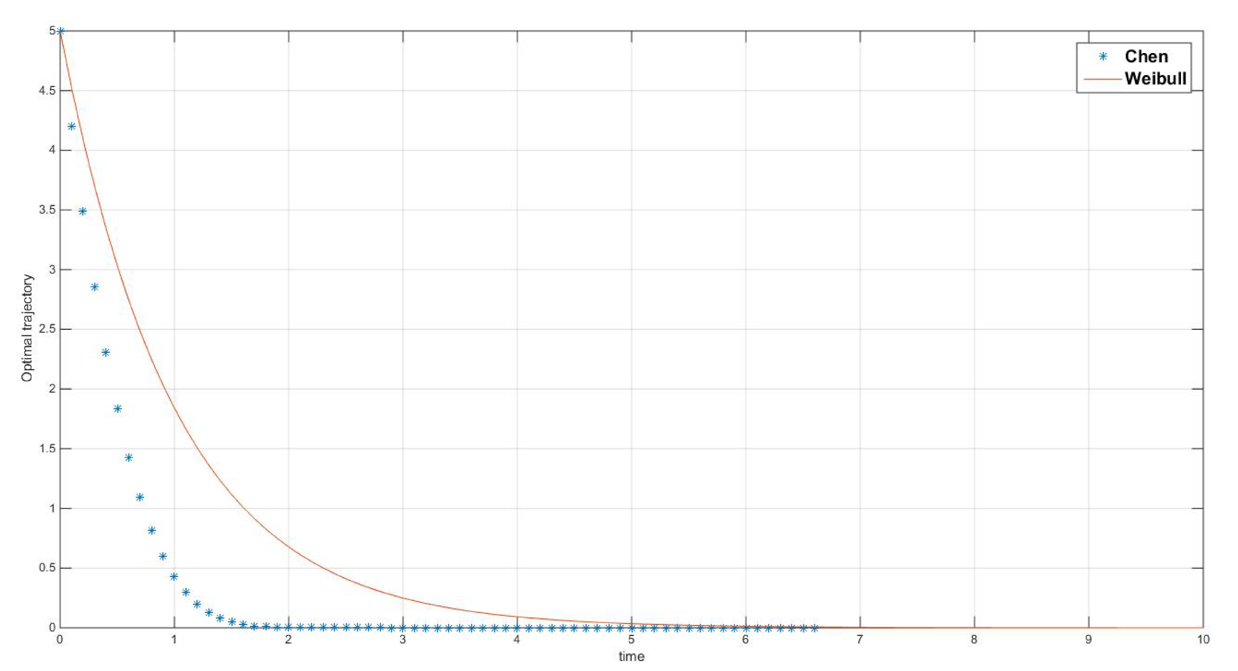
Figure 4, Figure 5 and Figure 6 summarize these results when ${\lambda }_1=1={\lambda }_2$, which, since ${\lambda }_1$ and ${\lambda }_2$ are scale parameters of the distributions under study, we can have a sufficiently general idea of our developments. The reason is that, if we select other values for these parameters, we will end up having constant multiples of the random variables $X_1$ and $X_2$ analyzed in this study (see Reference [60] ( Section 4.2.1)).

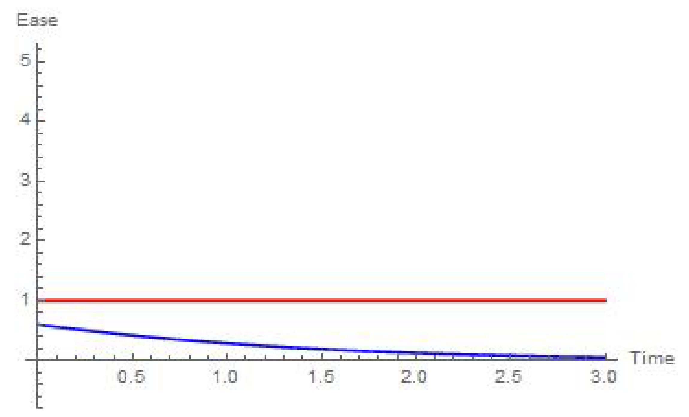
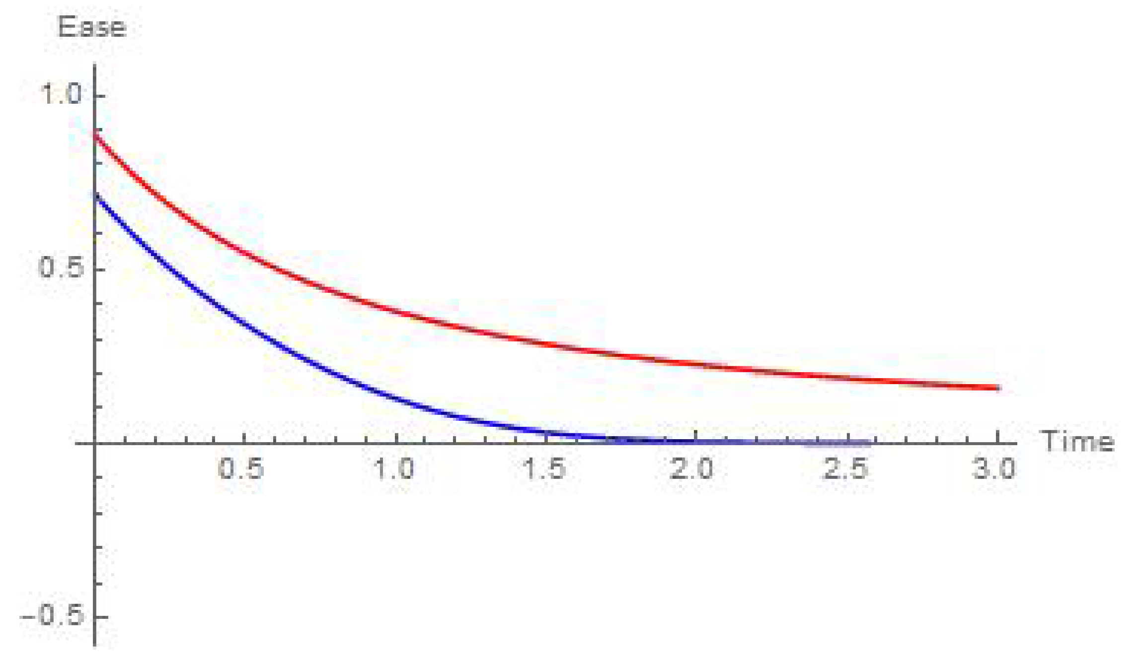
We might give a plausible interpretation of Figure 5 and Figure 6 in the direction of Remark 2. The optimal extraction rates are linear in the state variable and, as we established in Remark 2(ii), the largest the value of $A\left(t\right)={\overline{a}}_t$ is, the easiest it is for the extractor to obtain $u^{*}(t,x)$. In this sense, it is straightforward that, for Chen’s law, as time goes by, it becomes harder to extract at a rate of $u^{*}(t,x)$. On the other hand, it is very easy to see that, under Weibull’s law, $A\left(t\right)\equiv 1$ (see References [12,57,61] (Example 5.2.1; p. 323; Chapter 8.10.1)). This implies that, in the normal mode, the agent whose random terminal time follows the Weibull distribution is indifferent to the moment of time when the extraction task takes place, and should only look at the remaining amount of the resource.

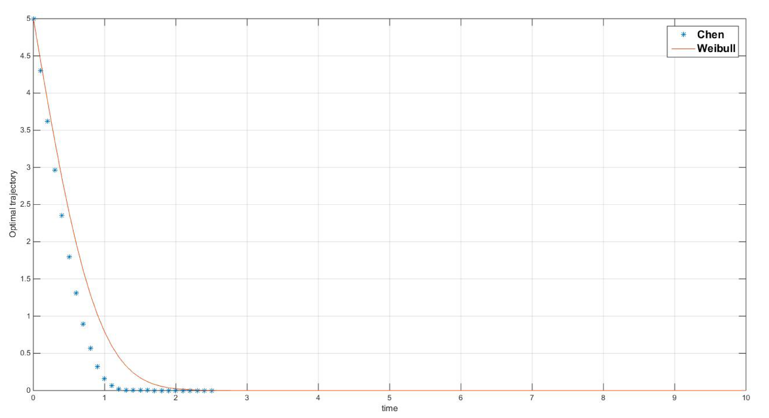
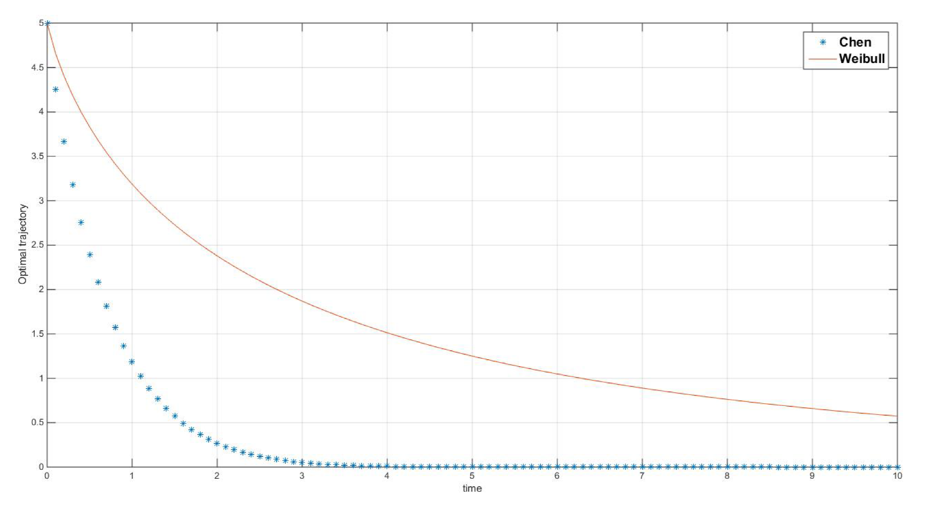
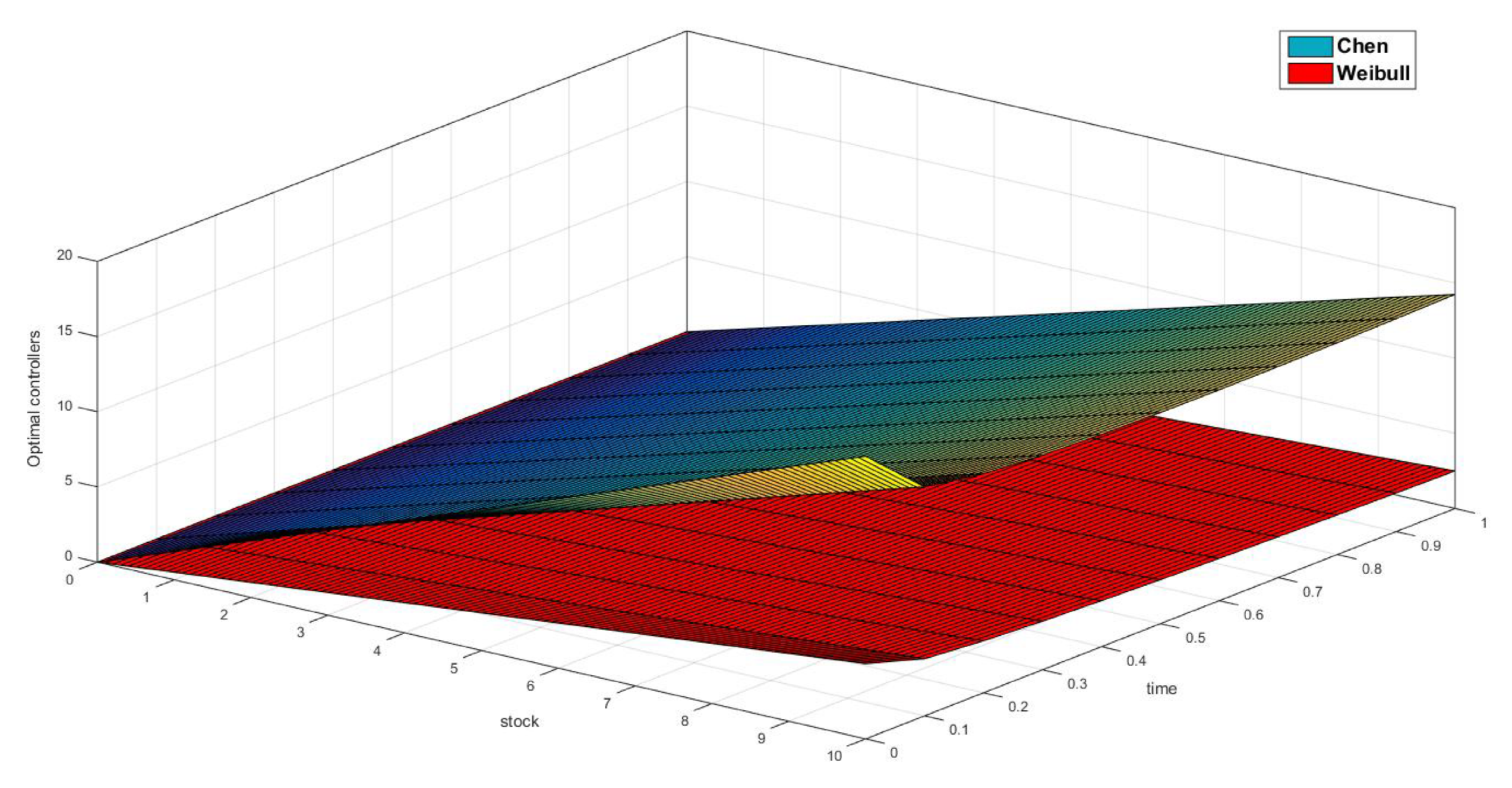
As for the optimal trajectories in Figure 4, observe that the system exploited by an agent affected by Chen’s law becomes exhausted a lot faster than a system exploited by a Weibull extractor. This is consistent with the fact that, according to Figure 5, a Chen extractor would be more intense in his exploitation tasks.

3.1.2. Aging Mode (${\delta }_1=2={\delta }_2$)

We stated before that for ${\delta }_1=2={\delta }_2$, Weibull’s law coincides with Rayleigh distribution. In this case, (20) gives that ${\lambda }_1\left(t\right)=2{\lambda }_{1}t$; then from Theorem 1 we get

$$\begin{array}{ccc}\hfill u^{*}(t,x)& =& \frac{x{\mathrm{e}}^{-{\lambda }_1{t}^2}}{{\int }_t^{\infty }{\mathrm{e}}^{-{\lambda }_1{s}^2}\mathrm{d}s}.\hfill \end{array}$$

For Chen’s distribution, when we have an aging system, by (22), the failure rate function is ${\lambda }_2\left(t\right)=2{\lambda }_{2}t{\mathrm{e}}^{t^2}$, and the Theorem 1 gives that the optimal control is

$$u^{*}(t,x)=\frac{xexp\left(-{\lambda }_2{\mathrm{e}}^{t^2}\right)}{{\int }_t^{\infty }exp\left(-{\lambda }_2{\mathrm{e}}^{s^2}\right)\mathrm{d}s}.$$

We solve (23) and get that the optimal trajectories under each law are:

$$x^{*}\left(\tau \right)=\left\{\begin{array}{ccc}{x}_{0}exp\left(-{\int }_0^{\tau }\frac{{\mathrm{e}}^{-{\lambda }_1{t}^2}}{{\int }_t^{\infty }{\mathrm{e}}^{-{\lambda }_1{s}^2}\mathrm{d}s}\mathrm{d}t\right)& \mathrm{for}{\mathrm{Weibull}}^{\prime }\mathrm{s}\mathrm{law}\mathrm{with}& {\delta }_1=2\\ x_{0}exp\left(-{\int }_0^{\tau }\frac{exp\left(-{\lambda }_2{\mathrm{e}}^{t^2}\right)}{{\int }_t^{\infty }exp\left(-{\lambda }_2{\mathrm{e}}^{s^2}\right)\mathrm{d}s}\mathrm{d}t\right)& \mathrm{for}{\mathrm{Chen}}^{\prime }\mathrm{s}\mathrm{law}\mathrm{with}& {\delta }_2=2.\end{array}\right.$$

Figure 7, Figure 8 and Figure 9 summarize these results when ${\lambda }_1=1={\lambda }_2$. There, we can see that, in the aging mode, as time passes by, the extraction tasks need to be more intense for both assumptions.

However, for the Chen extractor, the situation deteriorates very rapidly, and hence, it needs to speed up the pace of its tasks. It readily follows from (29) that both controllers are linear in the state. Again, Figure 7 shows how the stock becomes exhausted for each case.

3.1.3. Early Period (${\delta }_1=\frac{1}{2}={\delta }_2$)

For the Weibull case, (20) yields that the hazard rate function is ${\lambda }_1\left(t\right)=\frac{{\lambda }_1}{2\sqrt{t}}$. A substitution in (29) gives us

$$\begin{array}{ccc}\hfill u^{*}(t,x)& =& \frac{x{\mathrm{e}}^{-{\lambda }_1\sqrt{t}}}{{\int }_t^{\infty }{\mathrm{e}}^{-{\lambda }_1\sqrt{s}}\mathrm{d}s}.\hfill \end{array}$$

For Chen’s law, the pre-run system has a hazard rate function of the form ${\lambda }_2\left(t\right)=\frac{{\lambda }_2}{2\sqrt{t}}{\mathrm{e}}^{\sqrt{t}}$. The corresponding optimal control has the form

$$\begin{array}{ccc}\hfill u^{*}(t,x)& =& \frac{xexp\left(-{\lambda }_2{\mathrm{e}}^{\sqrt{t}}\right)}{{\int }_t^{\infty }exp\left(-{\lambda }_2{\mathrm{e}}^{\sqrt{s}}\right)\mathrm{d}s}.\hfill \end{array}$$

We solve (23) and get that the optimal trajectories under each law are:

$$x^{*}\left(\tau \right)=\left\{\begin{array}{ccc}{x}_{0}exp\left(-{\int }_0^{\tau }\frac{{\lambda }_1^2}{2({\lambda }_1\sqrt{\tau }+1)}\mathrm{d}t\right)& \mathrm{for}{\mathrm{Weibull}}^{\prime }\mathrm{s}\mathrm{law}\mathrm{with}& {\delta }_1=\frac{1}{2},\\ x_{0}exp\left(-{\int }_0^{\tau }\frac{exp\left(-{\lambda }_2{\mathrm{e}}^{\sqrt{t}}\right)}{{\int }_t^{\infty }exp\left(-{\lambda }_2{\mathrm{e}}^{\sqrt{s}}\right)\mathrm{d}s}\mathrm{d}t\right)& \mathrm{for}{\mathrm{Chen}}^{\prime }\mathrm{s}\mathrm{law}\mathrm{with}& {\delta }_2=\frac{1}{2}.\end{array}\right.$$

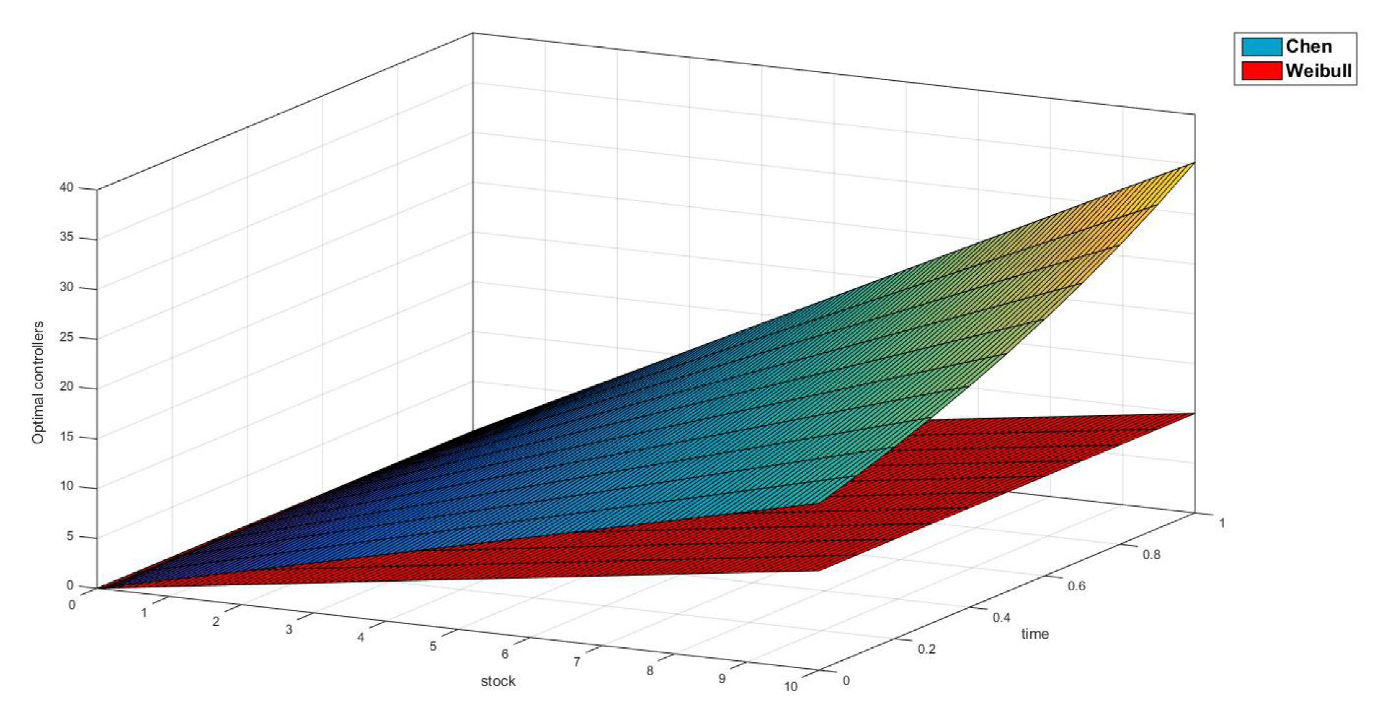
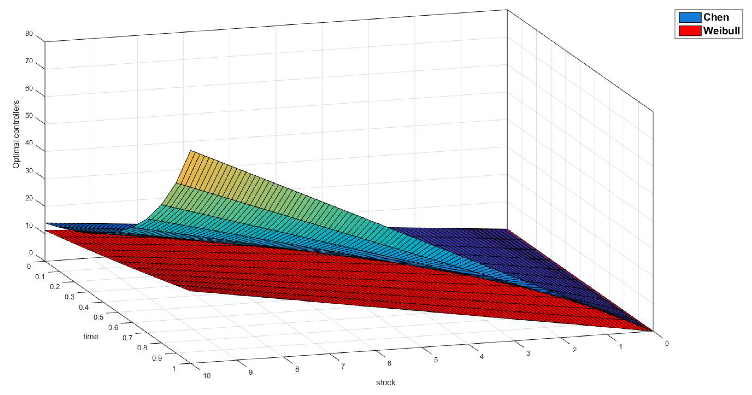
Figure 10, Figure 11 and Figure 12 summarize these results when $\lambda =1$. It is of particular interest that, according to Figure 12, for a Chen extractor, we almost have the same situation displayed in Figure 6 with the Weibull extractor. However, in this case, the intensity function $A\left(t\right)={\overline{a}}_t$ converges to a smaller value than the one displayed in that part of the illustration. This means that, during the early mode of the system, an agent whose random terminal time follows the Chen distribution should only mind about the remaining stock of the resource.

For a Weibull extractor at the pre-run phase, as time goes by, the exploitation becomes less intense, and, in spite of the fact that the reserve will be consumed at an exponential rate, it will last for more time than under Chen assumption (look at Figure 10). An economic interpretation of this fact is that the optimal rules of behavior for the agents demand Chen’s law to be more intense in its labors even from the early period, while they allow Weibull’s to be less intense (look at Figure 11).

3.2. Game Theoretic Model for the Extraction of Natural Resources

Now we consider the non degenerate game model from Section 2. For that purpose, we will make an extensive use of the results presented in References [1,50] and [57] (Chapter 9.2). Note that the utility function of the agent will explicitly depend only on its own control, and there are no payoff transfers among the players, that is, on the extraction rate applied by the agent, and on the stock of the resource at time $t\ge 0$.

Theorem 3.1 in Reference [1] allows us to state the HJBI equations associated with the optimization problem for the i-th player. Namely,

$$\begin{array}{c}-\frac{\partial }{\partial t}{W}_i(x,t)+({\lambda }_1\left(t\right)+{\lambda }_2\left(t\right))W_i(x,t)\hfill \end{array}$$

$$\begin{array}{c}=\underset{u_i\in {\Pi }^i}{max}\left(h_i(t,u_1,u_2)+{\mathsf{\Phi }}_i\left(x\right){\lambda }_j\left(t\right)-\frac{\partial }{\partial x}{W}_i(x,t)(u_1+u_2)\right),\hfill \end{array}$$

(43)

$$\begin{array}{c}{W}_i(x,t)\to 0ast\to \infty ,\hfill \end{array}$$

(44)

for $i=1,2$.

We will find explicit solutions for (43) when the functions $h_i$ are analogous to (28) for $i=1,2$. That is, when

$$h_i(x,u_1(t,x),u_2(t,x))=ln\left(u_i(t,x)\right).$$

(45)

We also suppose that

$${\mathsf{\Phi }}_i\left(x(t\wedge \tau )\right)=c_{i}ln\left(x(t\wedge \tau )\right)=c_{i}ln\left(x\right){\chi }_{\tau \le t},$$

(46)

for some positive constant values $c_i$ and $i=1,2$. In this case, the HJBI Equation (43) turns out to be

$$\begin{array}{c}-\frac{\partial }{\partial t}{W}_i(x,t)+({\lambda }_1\left(t\right)+{\lambda }_2\left(t\right))W_i(x,t)\hfill \\ =\underset{u_i\in {\Pi }^1}{max}\left(ln\left(u_i\right)+c_{i}ln\left(x\right){\lambda }_{-i}\left(t\right)-\frac{\partial }{\partial x}{W}_i(x,t)(u_1+u_2)\right),\hfill \end{array}$$

for $i=1,2$. Here,

$${\lambda }_{-i}(·):=\left\{\begin{array}{cc}{\lambda }_2(·)& \mathrm{if}i=1,\\ {\lambda }_1(·)& \mathrm{if}i=2.\end{array}\right.$$

In what follows, we find the optimal strategies and the value function for this problem by proceeding in the same way that led us to (29) and (41). The next result is similar to Reference [1] (Proposition 4.1).

Theorem 3.

If the utility functions are of the form (28), and the terminal payoff functions are given by (46), then the optimal strategies for the game $\mathsf{\Gamma }\left(x_0\right)$ are Lebesgue-measurable, and are given by:

$$u_i^{*}(t,x)=\frac{x}{{\overline{a}}_{{\left[t\right]}_1:{\left[t\right]}_2}+c_i{\overline{A}}_{{\left[t\right]}_i:}{}_{{\left[t\right]}_{-i}}^1},$$

(47)

for $i=1,2$, where

$${\overline{a}}_{{\left[t\right]}_1:{\left[t\right]}_2}:={\int }_0^{\infty }\frac{1-F(t+s)}{1-F\left(t\right)}\mathrm{d}s,$$

(48)

and

$${\overline{A}}_{{\left[t\right]}_i:}{}_{{\left[t\right]}_{-i}}^1:={\int }_0^{\infty }\frac{1-F(t+s)}{1-F\left(t\right)}{\lambda }_{-i}(s+t)\mathrm{d}s.$$

(49)

Here, $F\left(t\right)$ is as in (5).

Proof. 

The substitution of the informed guesses

$$W_i(x,t)=A_i\left(t\right)lnx+B_i\left(t\right),$$

for $i=1,2$; into (43) and (44) yields:

• that the maximizers of (43) are of the form

  $$u_i^{*}(t,x)=\frac{x}{A_i\left(t\right)}.$$

  (50)
  The fact that these controllers are Lebesgue-measurable follows from Hypothesis 1(b), along with the so-named measurable selection theorems (see, for instance, References [69,70,71] (Theorem 12.1; Proposition D5(a); Theorem 3.4)).
• the following Cauchy problem (which is analogous to (35)–(38)):

  $$\begin{array}{ccc}\hfill -{\dot{A}}_i\left(t\right)+A_i\left(t\right)({\lambda }_i\left(t\right)+{\lambda }_{-i}\left(t\right))& =& 1+c_i{\lambda }_{-i}\left(t\right),\hfill \end{array}$$

  (51)

  $$\begin{array}{ccc}\hfill {\dot{B}}_i\left(t\right)-B_i\left(t\right)({\lambda }_i\left(t\right)+{\lambda }_{-i}\left(t\right))& =& ln{A}_i\left(t\right)+1+\frac{A_i\left(t\right)}{A_{-i}\left(t\right)}\hfill \end{array}$$

  (52)

  $$\begin{array}{ccc}\hfill \underset{t\to \infty }{lim}{A}_i\left(t\right)& =& 0,\hfill \end{array}$$

  (53)

  $$\begin{array}{ccc}\hfill \underset{t\to \infty }{lim}{B}_i\left(t\right)& =& 0.\hfill \end{array}$$

  (54)

We apply the technique of the integrating factor in (51); use the transversality condition (53), and get

$$\begin{array}{ccc}\hfill A_i\left(t\right)& =& \frac{{\int }_t^{\infty }(1+c_i{\lambda }_{-i}\left(\tau \right))exp\left(-{\int }_0^{\tau }{\lambda }_i\left(s\right)+{\lambda }_{-i}\left(s\right)\mathrm{d}s\right)\mathrm{d}\tau }{exp\left(-{\int }_0^t{\lambda }_i\left(\tau \right)+{\lambda }_{-i}\left(\tau \right)\mathrm{d}\tau \right)}\hfill \\ & =& \frac{{\int }_t^{\infty }(1+c_i{\lambda }_{-i}\left(\tau \right))(1-F\left(\tau \right))\mathrm{d}\tau }{1-F\left(t\right)}.\hfill \end{array}$$

The last equality holds by virtue of (5).

We now use (48) and (49) and observe that

$$A_i\left(t\right)={\overline{a}}_{{\left[t\right]}_1:{\left[t\right]}_2}+c_i{\overline{A}}_{{\left[t\right]}_i:}{}_{{\left[t\right]}_{-i}}^1.$$

(55)

The substitution of this expression in (50) yields (47).

By Theorem I.7.1(a) in Reference [68] (see also Reference [52] (Theorem 2(i))), we know that (47) is optimal for the game with no explicit payoff transfer among the players. This proves the result. □

Remark 3.

Just as we interpreted (39) in Remark 2 as a continuous life annuity, we can do the same with (55).

• In the Actuarial Mathematics literature, the continuous annuity of the joint-life status of the times-until-failure $T_1$ and $T_2$ is designed by the symbol ${\overline{a}}_{{\left[t\right]}_1:}{}_{{\left[t\right]}_2}$, and represents a natural extension of (30) to the case where the payments stop when either player leaves the system (the use of the braces around t emphasizes the fact that each player has lived-up to the moment $t>0$, and states that the age-at-selection of each player is t—see Reference [57] (Chapter 3.8)). Thus we define such annuity as in (48) (with null interest rate);
• we also design the mathematical expectation of the present value of one monetary unit payable (to the i-th player) at the moment of failure of the $(-i)$-th player (with null interest rate) by the symbol ${\overline{A}}_{{\left[t\right]}_i:}{}_{{\left[t\right]}_{-i}}^1$, as in (49) (the superscript 1 means that the $(-i)$-th player is the first who fails—see Reference [57] (Chapter 9.7)). The reason is that the expression

  $$\frac{1-F(t+s)}{1-F\left(t\right)}{\lambda }_{-i}(s+t)$$

  can be thought of as the probability that both agents survive up to moment t, and the $(-i)$-th agent fails at moment $t+s$. (See References [46,57] (Chapter 9.9)).

Keeping this in mind we can propose an extension of (40) and write (47) as:

$$x-u_i^{*}(t,x)·\left({\overline{a}}_{{\left[t\right]}_1:{\left[t\right]}_2}+c_i{\overline{A}}_{{\left[t\right]}_i:}{}_{{\left[t\right]}_{-i}}^1\right)=0.$$

(56)

From an actuarial perspective, this expression means that, for the i-th extractor, there is a balance between the eventual benefit x, and the continuous rate of extraction $u_i^{*}(t,x)$, which includes a final payment (of size $c_i{u}_i^{*}(t,x)$) that covers the possibility that the other player fails and leaves the game.

This means that the optimal rate of extraction of the i-th player in (47) can be viewed as the composition of two parts:

(i) 

the benefit that the agent will eventually get, x; and

(ii) 

the intensity of the effort that the agent needs to apply to attain such benefit, that is, (55). Observe that this function explicitly takes into account the fact that the i-th agent will receive a payment if the other one leaves the system before he/she does.

The resulting utility of this exercise for the i-th player is given by (45).

As a by-product of Theorem 3, we can state and prove the following result.

Theorem 4.

If the utility functions are of the form (28), and the terminal payoff functions are given by (46), then the value functions for game $\mathsf{\Gamma }\left(x_0\right)$ are given by

$$\begin{array}{c}{W}_i(x,t)=\left({\overline{a}}_{{\left[t\right]}_1:{\left[t\right]}_2}+c_i{\overline{A}}_{{\left[t\right]}_i:}{}_{{\left[t\right]}_{-i}}^1\right)lnx\hfill \\ +{\int }_0^{\infty }\left(1+ln\left({\overline{a}}_{{\left[t\right]}_1+s:{\left[t\right]}_2+s}+c_i{\overline{A}}_{{\left[t\right]}_i+s:}{}_{{\left[t\right]}_{-i}+s}^1\right)+\frac{{\overline{a}}_{{\left[t\right]}_1+s:{\left[t\right]}_2+s}+c_i{\overline{A}}_{{\left[t\right]}_i+s:}{}_{{\left[t\right]}_{-i}+s}^1}{{\overline{a}}_{{\left[t\right]}_1+s:{\left[t\right]}_2+s}+c_{-i}{\overline{A}}_{{\left[t\right]}_i+s:}^1{}_{{\left[t\right]}_{-i}+s}}\right)\frac{1-F(s+t)}{1-F\left(t\right)}\mathrm{d}s,\hfill \end{array}$$

for $i=1,2$.

Proof. 

From Theorem 3, we readily know that

$$W_i(x,t)=\left({\overline{a}}_{{\left[t\right]}_1:{\left[t\right]}_2}+c_i{\overline{A}}_{{\left[t\right]}_i:}{}_{{\left[t\right]}_{-i}}^1\right)lnx+B_i\left(t\right),$$

for $i=1,2$. To find the functions $B_i\left(t\right)$, we apply the technique of the integrating factor to (52), and use the transversality condition (54). This gives:

$$\begin{array}{ccc}\hfill B_i\left(t\right)& =& \frac{{\int }_t^{\infty }\left(ln{A}_i\left(s\right)+1+\frac{A_i\left(s\right)}{A_{-i}\left(s\right)}\right)exp\left(-{\int }_0^s{\lambda }_i\left(\tau \right)+{\lambda }_{-i}\left(\tau \right)\mathrm{d}\tau \right)\mathrm{d}s}{exp\left(-{\int }_0^t{\lambda }_i\left(s\right)+{\lambda }_{-i}\left(s\right)\mathrm{d}s\right)},\hfill \\ & =& \frac{{\int }_t^{\infty }\left(ln{A}_i\left(s\right)+1+\frac{A_i\left(s\right)}{A_{-i}\left(s\right)}\right)(1-F\left(s\right))\mathrm{d}s}{1-F\left(t\right)},\hfill \end{array}$$

where $A_i(·)$ is as in (55).

The optimality of the functions $W_1$ and $W_2$ follows from Reference [52] (Theorem 2(ii)). This completes the proof. □

The optimal trajectory can be found by plugging (47) into (1) and solving. That is,

$$x^{*}\left(\tau \right)=x_{0}exp\left(-\sum _{i=1}^2{\int }_0^{\tau }\frac{exp\left(-{\int }_0^t({\lambda }_1\left(s\right)+{\lambda }_2\left(s\right))\mathrm{d}s\right)}{{\int }_t^{\infty }(1+c_i{\lambda }_{-i}\left(s\right))exp\left(-{\int }_0^s({\lambda }_1\left(r\right)+{\lambda }_2\left(r\right))\mathrm{d}r\right)\mathrm{d}s}\mathrm{d}t\right).$$

(57)

The relation (57) can also be compactly written as

$$x^{*}\left(\tau \right)=x_0\exp \left(-{\int }_0^{\tau }\frac{1}{{\overline{a}}_{{\left[t\right]}_1:{\left[t\right]}_2}+c_1{\overline{A}}_{{\left[t\right]}_1:}{}_{{\left[t\right]}_2}^1}+\frac{1}{{\overline{a}}_{{\left[t\right]}_1:{\left[t\right]}_2}+c_2{\overline{A}}_{{\left[t\right]}_1:}^1{}_{{\left[t\right]}_2}}\mathrm{d}t\right),$$

thus showing the interaction between the players and their effect on the system.

3.3. An Illustration

We devote this Section to the analysis of the particular cases of our interest.

If the random terminal time of player 1 has a Weibull distribution, and that of player 2 follows Chen’s law, the optimal extraction rates are:

$$u_1^{*}(t,x)=\frac{xexp\left(-{\int }_0^t({\lambda }_1{\delta }_1{s}^{{\delta }_1-1}+{\lambda }_2{\delta }_2{s}^{{\delta }_2-1}{\mathrm{e}}^{s^{{\delta }_2}})\mathrm{d}s\right)}{{\int }_t^{\infty }(1+c_1{\lambda }_2{\delta }_2{s}^{{\delta }_2-1}{\mathrm{e}}^{s^{{\delta }_2}})exp\left(-{\int }_0^s({\lambda }_1{\delta }_1{r}^{{\delta }_1-1}+{\lambda }_2{\delta }_2{r}^{{\delta }_2-1}{\mathrm{e}}^{r^{{\delta }_2}})\mathrm{d}r\right)\mathrm{d}s},$$

and

$$u_2^{*}(t,x)=\frac{xexp\left(-{\int }_0^t({\lambda }_1{\delta }_1{s}^{{\delta }_1-1}+{\lambda }_2{\delta }_2{s}^{{\delta }_2-1}{\mathrm{e}}^{s^{{\delta }_2}})\mathrm{d}s\right)}{{\int }_t^{\infty }(1+c_2{\lambda }_1{\delta }_1{s}^{{\delta }_1-1})exp\left(-{\int }_0^s({\lambda }_1{\delta }_1{r}^{{\delta }_1-1}+{\lambda }_2{\delta }_2{r}^{{\delta }_2-1}{\mathrm{e}}^{r^{{\delta }_2}})\mathrm{d}r\right)\mathrm{d}s}.$$

If we fix the initial stock at $x_0=5$, Figure 13, Figure 14, Figure 15, Figure 16, Figure 17 and Figure 18 will show us a graphical depiction of the involved intensities in the process. From these images, we can notice that almost all the time the extraction rates of the player whose random terminal time follows the Chen distribution are higher than those of the other player. This fact is also consistent with the plots of Figure 4, Figure 5 and Figure 6 and Figure 10, Figure 11 and Figure 12, which were exhibited in the illustration of Section 3.

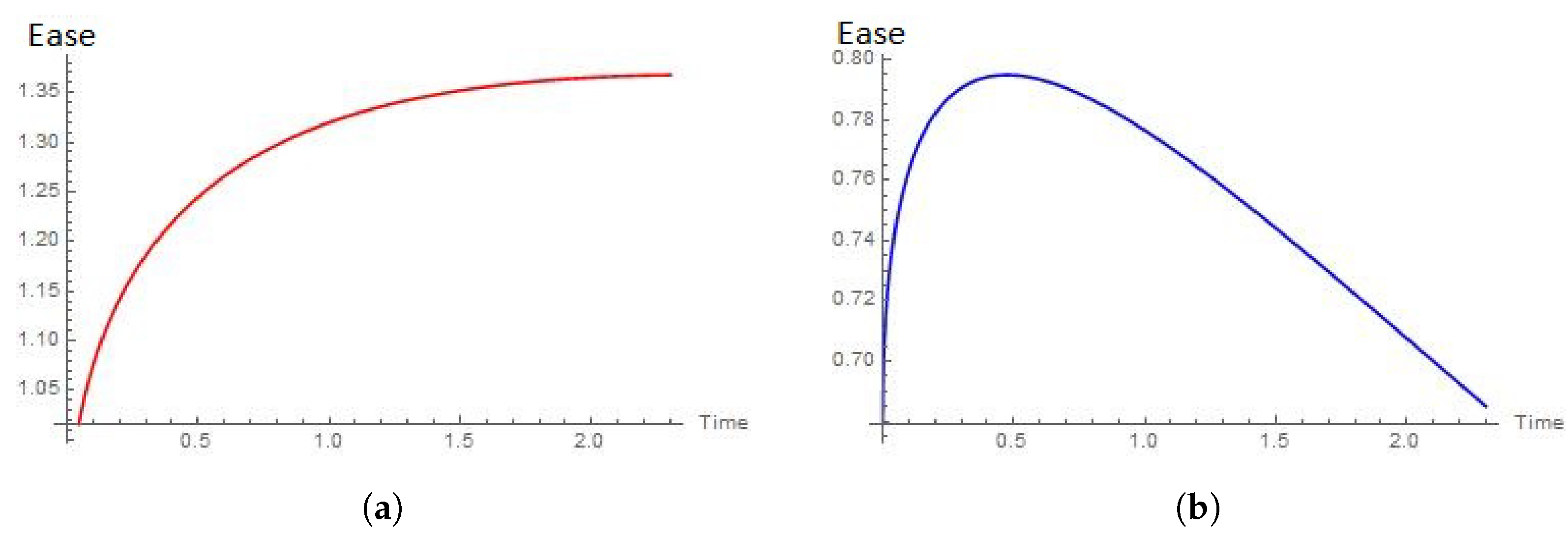
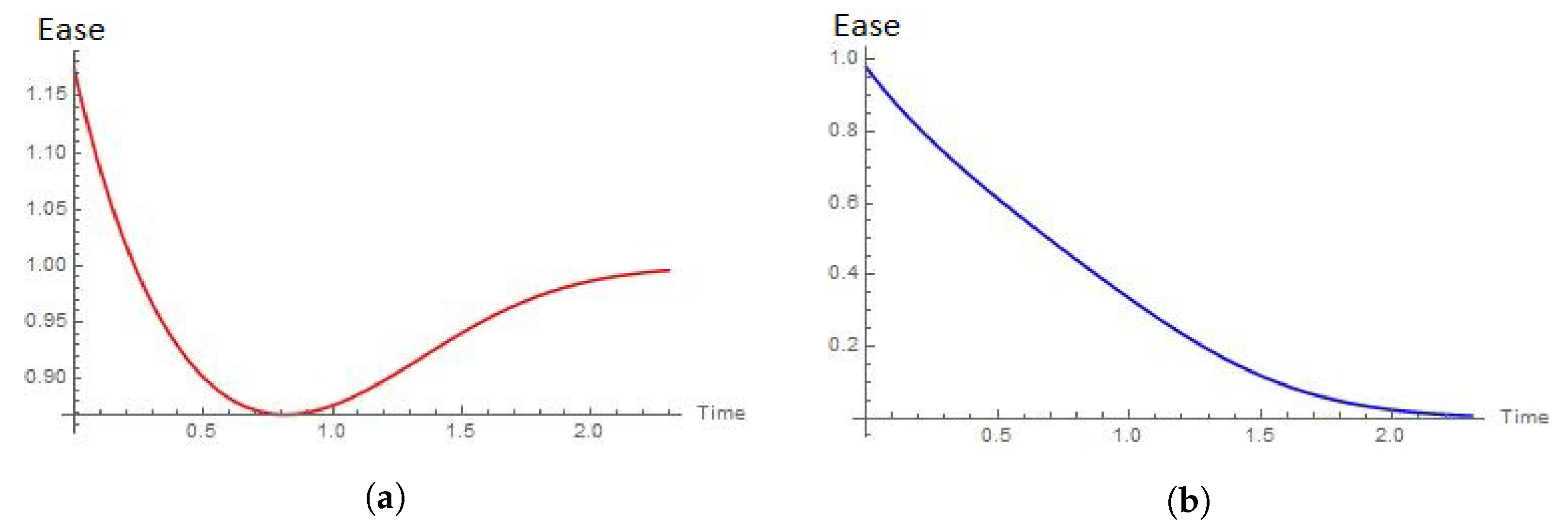
To have a proper interpretation of the results presented in Figure 13, recall Figure 10, Figure 11 and Figure 12. Observe that the shapes of the plots in Figure 13a,b resemble those in Figure 12. It should be noted that the scales are much larger in the degenerate case. The reason is that, in this scenario, there are two actors making decisions and consuming the resource. Moreover, each of the agents needs to take into consideration the action of its counterpart (recall Theorem 3). As in the one-player case, it should be noticed that, in spite of the fact that the plots in Figure 13a,b have opposite trends, the optimal behavior of the Chen extractor is to obtain the resource at a much rapid pace than that of the Weibull extractor.

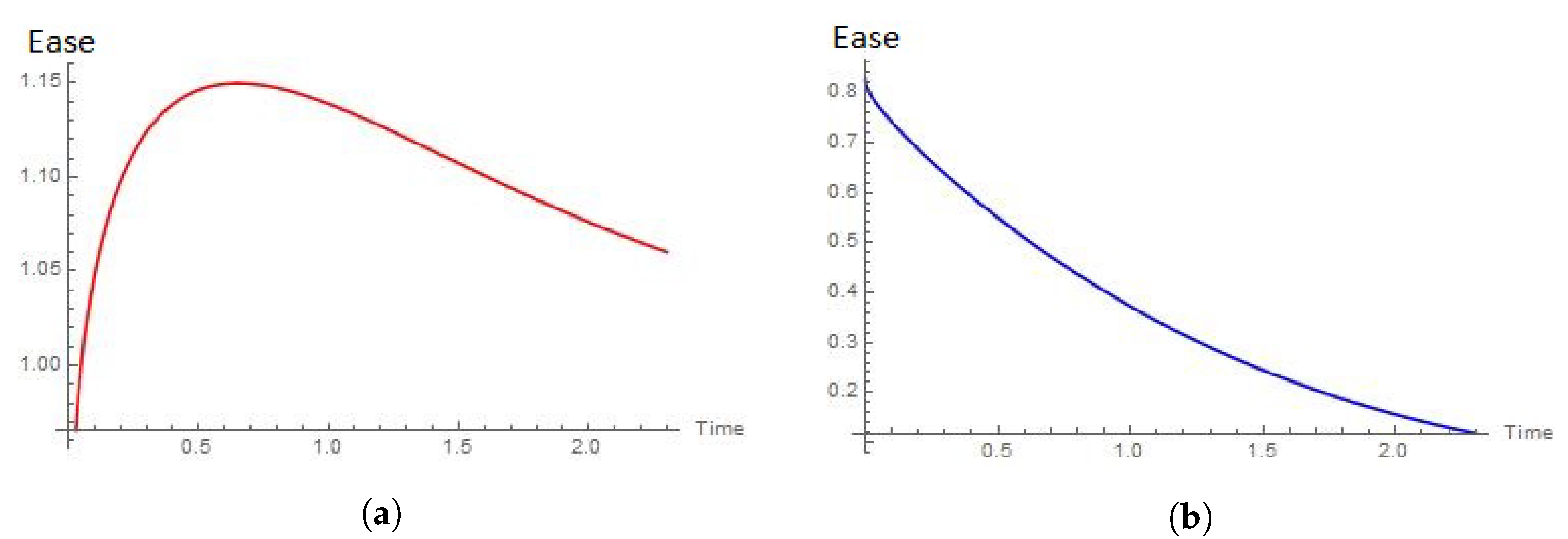
In view of Figure 14, we must recall Figure 4, Figure 5 and Figure 6 and Figure 10, Figure 11 and Figure 12. Again, for the intensity function of the Chen extractor, $A_2(·)$, we see the same general trend as that in Figure 6. However, for the Weibull case, the trend observed in Figure 12 becomes perturbed by the presence of the other agent in a more advanced mode of the extraction.

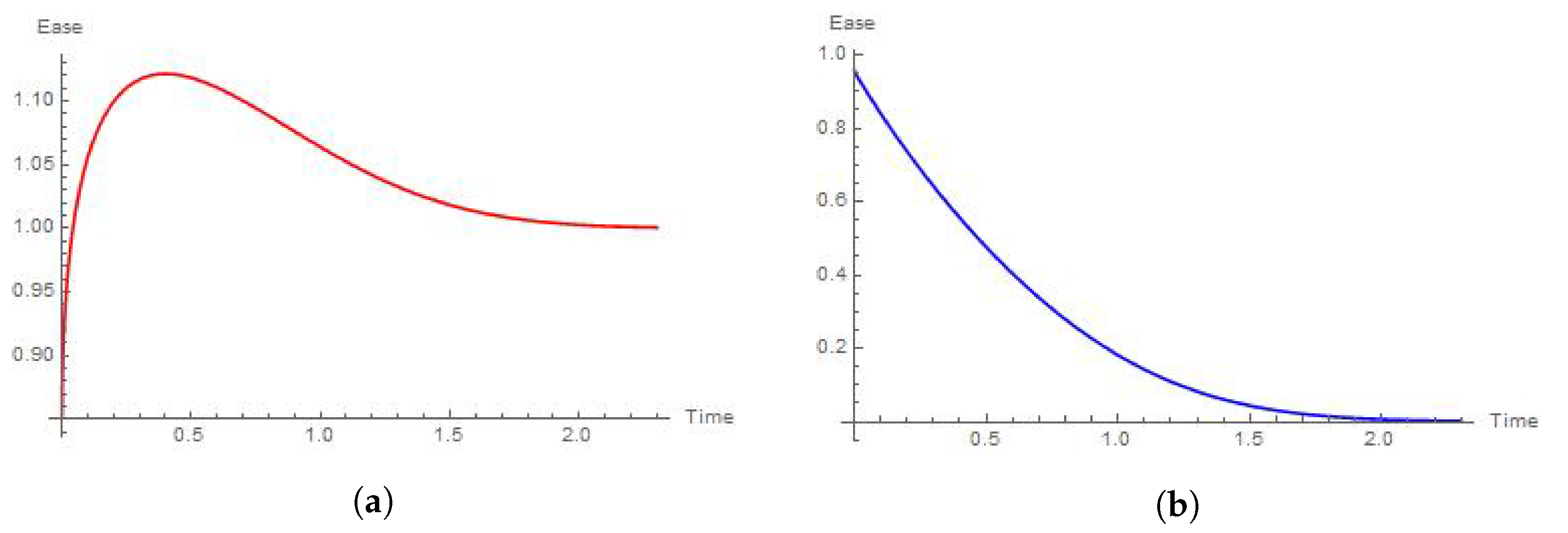
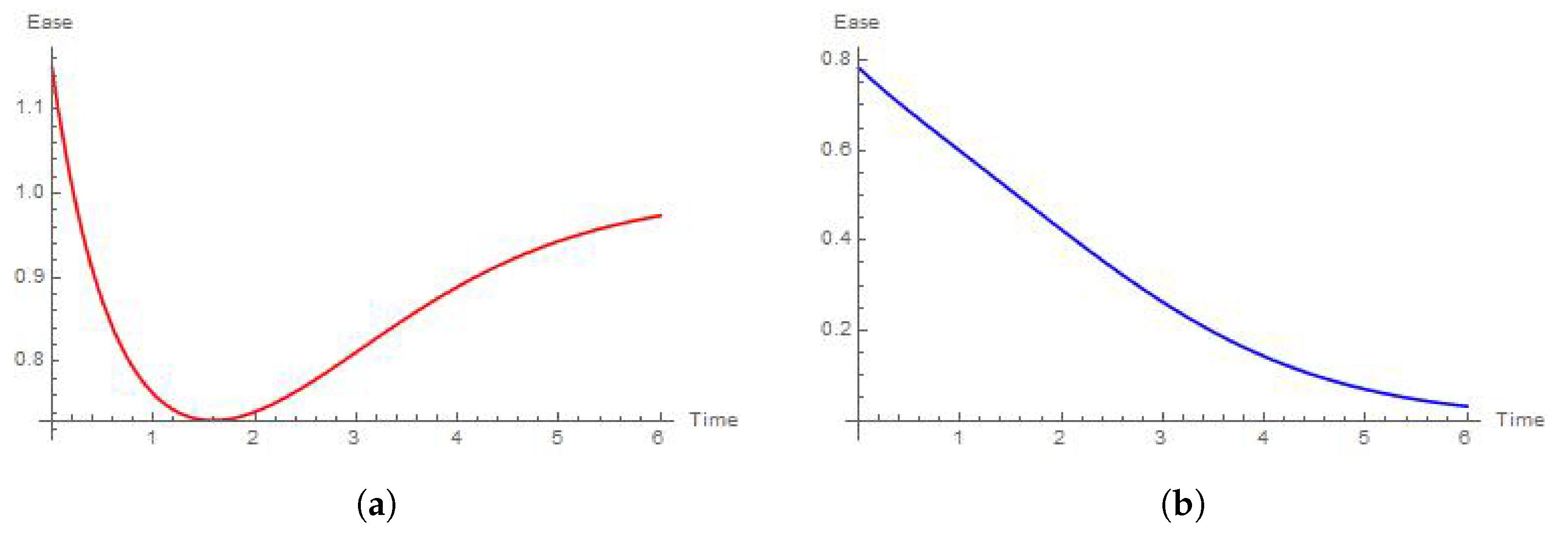
Figure 15 can be interpreted by means of Figure 7, Figure 8, Figure 9, Figure 10, Figure 11 and Figure 12. Note that from the comparison of Figure 15a with Figure 12 it is very clear how the presence of the Chen extractor affects the ease of the extraction of Weibull’s player.

For the case ${\delta }_1=1$, we present the following result.

Proposition 2.

If ${\delta }_1=1$, then

$$A_1\left(t\right)=c_1+(1-c_1{\lambda }_1)\frac{{\mathrm{e}}^t}{1-F_2\left(t\right)}\left(\frac{1}{{\lambda }_1}-\mathcal{L}\left(F_2\right)\right),$$

where $\mathcal{L}\left(F_2\right):={\int }_0^{\infty }{\mathrm{e}}^{-{\lambda }_1\tau }{F}_2\left(\tau \right)\mathrm{d}\tau$ stands for the Laplace transform of the distribution function $F_2$.

Proof. 

By (55), we readily know that

$$A_1\left(t\right)={\overline{a}}_{{\left[t\right]}_1:{\left[t\right]}_2}+c_1{\overline{A}}_{{\left[t\right]}_1}{}_{{\left[t\right]}_2}^1.$$

(58)

Now, by (5) and (48) (with $v\equiv 1$) we can write

$$\begin{array}{ccc}\hfill {\overline{a}}_{{\left[t\right]}_1:{\left[t\right]}_2}& =& {\int }_0^{\infty }\frac{1-F_1(t+\tau )}{1-F_1\left(t\right)}\frac{1-F_2(t+\tau )}{1-F_2\left(t\right)}\mathrm{d}\tau \hfill \\ & =& {\int }_0^{\infty }{\mathrm{e}}^{-{\lambda }_1\tau }\frac{1-F_2(t+\tau )}{1-F_2\left(t\right)}\mathrm{d}\tau .\hfill \end{array}$$

The last equality follows from plugging ${\delta }_1=1$ into Weibull’s distribution. Define $s_2\left(\tau \right):=\frac{1-F_2(t+\tau )}{1-F_2\left(t\right)}$ as the conditional survival of the random variable $[T-t|T>t]$ and write

$${\overline{a}}_{{\left[t\right]}_1:{\left[t\right]}_2}={\int }_0^{\infty }{\mathrm{e}}^{-{\lambda }_1\tau }{s}_2\left(\tau \right)\mathrm{d}\tau .$$

(59)

We now use (5) and (49) (with $v\equiv 1$) to write

$$\begin{array}{ccc}\hfill {\overline{A}}_{{\left[t\right]}_1:}{}_{{\left[t\right]}_2}^1& =& {\int }_0^{\infty }\frac{1-F_1(t+\tau )}{1-F_1\left(t\right)}\frac{1-F_2(t+\tau )}{1-F_2\left(t\right)}{\lambda }_2(t+\tau )\mathrm{d}\tau \hfill \\ & =& {\int }_0^{\infty }{\mathrm{e}}^{-{\lambda }_1\tau }\frac{1-F_2(t+\tau )}{1-F_2\left(t\right)}{\lambda }_2(t+\tau )\mathrm{d}\tau .\hfill \end{array}$$

The last equality follows from the substitution of ${\delta }_1=1$. Now, by the results in Reference [57] (Chapter 3.2.4) we can argue that

$${\overline{A}}_{{\left[t\right]}_1:}{}_{{\left[t\right]}_2}^1=-{\int }_0^{\infty }{\mathrm{e}}^{-\lambda \tau }{s}_2^{\prime }\left(\tau \right)\mathrm{d}\tau ,$$

(60)

where $s_2^{\prime }$ stands for the derivative of $s_2$. Plugging (59) and (60) into (58) yields

$$\begin{array}{ccc}\hfill A_1\left(t\right)& =& {\int }_0^{\infty }{\mathrm{e}}^{-{\lambda }_1\tau }(s_2\left(\tau \right)-c_1{s}_2^{\prime }\left(\tau \right))\mathrm{d}\tau \hfill \\ & =& \mathcal{L}(s_2-c_1{s}_2^{\prime })\hfill \\ & =& \mathcal{L}\left(s_2\right)-c_1\mathcal{L}\left(s_2^{\prime }\right)\hfill \\ & =& \mathcal{L}\left(s_2\right)-c_1({\lambda }_1\mathcal{L}\left(s_2\right)-s_2\left(0\right)).\hfill \end{array}$$

(61)

The last equality follows from the rule of Laplace Transform of Derivatives (see Reference [72] (Theorem 6.2.1)). Noting that $s_2\left(0\right)=1$ and rearranging the terms in (61) gives us

$$\begin{array}{ccc}\hfill A_1\left(t\right)& =& c_1+(1-c_1{\lambda }_1)\mathcal{L}\left(s_2\right)\hfill \\ & =& c_1+(1-c_1{\lambda }_1){\int }_0^{\infty }{\mathrm{e}}^{-{\lambda }_1\tau }\frac{1-F_2(t+\tau )}{1-F_2\left(t\right)}\mathrm{d}\tau \hfill \\ & =& c_1+(1-c_1{\lambda }_1){\int }_0^{\infty }{\mathrm{e}}^{-{\lambda }_1\tau }\frac{1-F_2(t+\tau )}{1-F_2\left(t\right)}\mathrm{d}\tau \hfill \\ & =& c_1+(1-c_1{\lambda }_1)\frac{{\mathrm{e}}^t}{1-F_2\left(t\right)}{\int }_0^{\infty }{\mathrm{e}}^{-{\lambda }_1\tau }(1-F_2\left(\tau \right))\mathrm{d}\tau \hfill \\ & =& c_1+(1-c_1{\lambda }_1)\frac{{\mathrm{e}}^t}{1-F_2\left(t\right)}\left(\frac{1}{{\lambda }_1}-\mathcal{L}\left(F_2\right)\right).\hfill \end{array}$$

This proves the result. □

Proposition 2 gives us that, regardless of the distribution of $T_2$ (or of its shape parameter for the case of Chen’s law), when $T_1$ follows the exponential distribution and $c_1{\lambda }_1=1$, the optimal rate of extraction will be invariant.

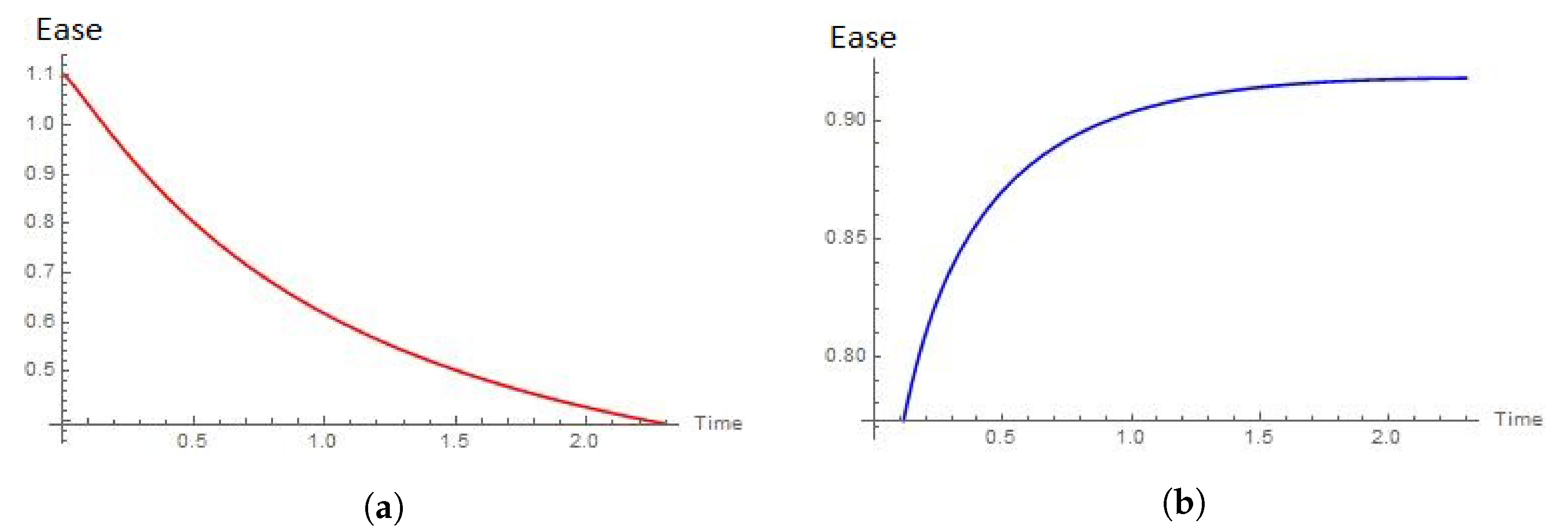
To interpret Figure 16, we recall Figure 7, Figure 8, Figure 9, Figure 10, Figure 11 and Figure 12. This case corresponds to the situation where the Weibull extractor is already at the aging mode of the process, and Chen extractor is only starting its tasks. Here, the intensity of Weibull’s extractor has to be higher as time passes, and the other player can take advantage of it because the intensity of its rate of extraction is decreasing. However, it is only at the beginning of the process when it is optimal for Chen extractor to have a stronger rate than that of Weibull (this is the only case in which this situation is observed). This is consistent with the behaviors shown by the intensity functions for the Weibull extractor in Figure 9, and for the Chen extractor in Figure 12.

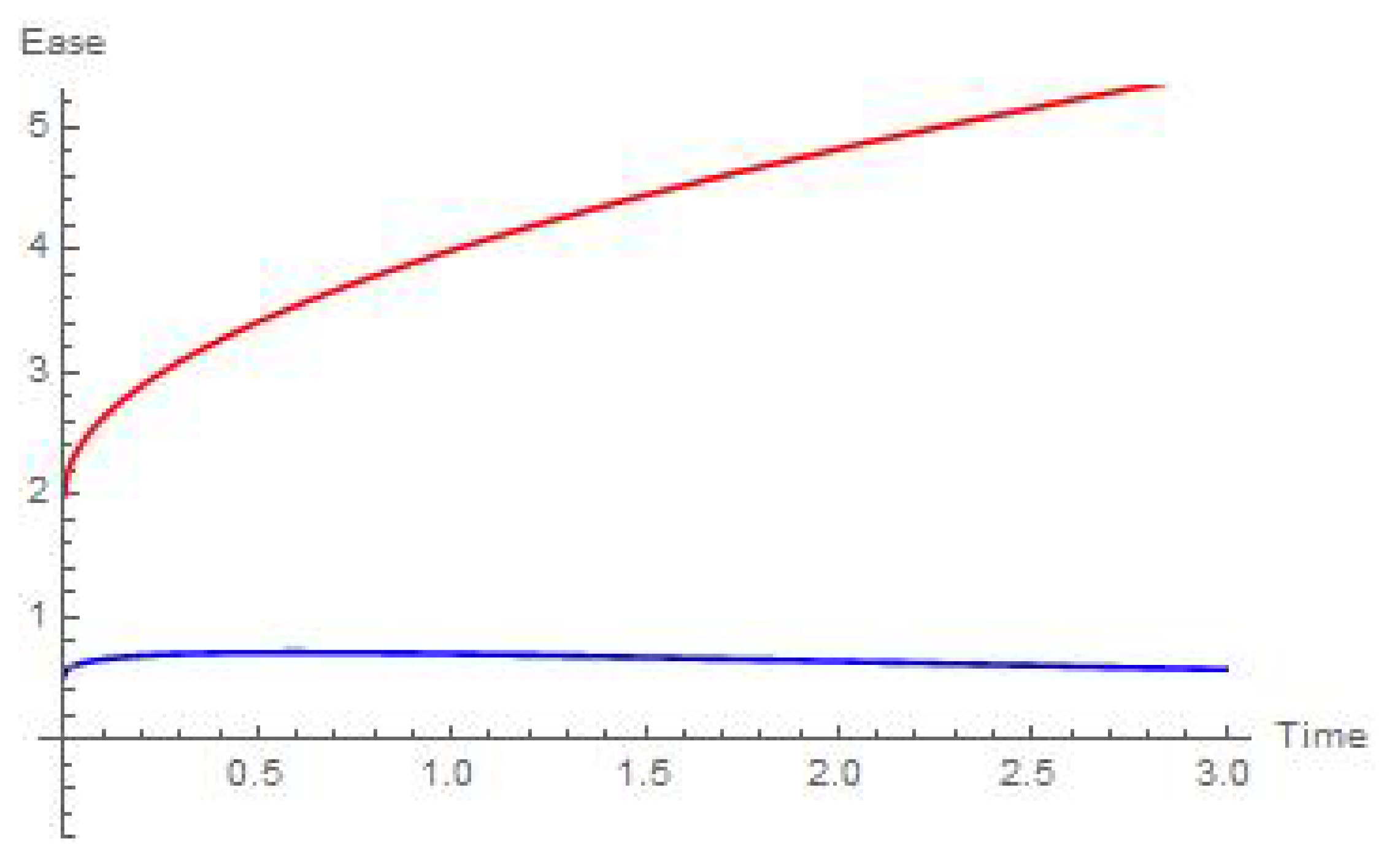
Figure 17a shows how the effort required by the Weibull extractor is a convex function that tends to stabilize in the long run. This feature is consistent with Figure 9. However, in the controlled case, we cannot observe an increasing trend. The behavior of the ease of Chen extractor mirrors that of the corresponding ease function in Figure 6.

Figure 18 shows a dramatized effect of the one shown in Figure 17. The reason is that both agents are in the aging mode of their respective processes.

If we fix the initial stock at $x_0=5$, and use Theorem 4, we can calculate the following table, where we have assumed, as in Section 3 that the scale parameters ${\lambda }_1$ and ${\lambda }_2$ equal the unity. Each of the entries represent the pair $(W_1(5,0),W_2(5,0))$.

Weibull/Chen	${\mathbf{\delta }}_{\mathbf{2}}=\frac{\mathbf{1}}{\mathbf{2}}$	${\mathbf{\delta }}_{\mathbf{2}}=\mathbf{1}$	${\mathbf{\delta }}_{\mathbf{2}}=\mathbf{2}$
${\delta }_1=\frac{1}{2}$	$(2.3257,1.4487)$	$(2.4326,1.6731)$	$(2.5882,1.9514)$
${\delta }_1=1$	$(2.5265,1.4734)$	$(2.6221,1.8187)$	$(2.7908,2.2097)$
${\delta }_1=2$	$(2.6941,1.5161)$	$(2.9190,1.9226)$	$(3.0567,2.4373)$

It should be noted that the player whose random terminal time is distributed according to the Chen’s law end’s up earning less than the other player in all cases. This is consistent with the comparisons we made in Section 2, and in particular, in Figure 3c.

The optimal trajectory is given by the following exponential function:

$$\begin{array}{ccc}\hfill x^{*}\left(\tau \right)& =& x_{0}exp(-{\int }_0^{\tau }\frac{exp\left(-{\int }_0^t({\lambda }_1{\delta }_1{s}^{{\delta }_1-1}+{\lambda }_2{\delta }_2{s}^{{\delta }_2-1}{\mathrm{e}}^{s^{{\delta }_2}})\mathrm{d}s\right)}{{\int }_t^{\infty }(1+c_1{\lambda }_2{\delta }_2{s}^{{\delta }_2-1}{\mathrm{e}}^{s^{{\delta }_2}})exp\left(-{\int }_0^s({\lambda }_1{\delta }_1{r}^{{\delta }_1-1}+{\lambda }_2{\delta }_2{r}^{{\delta }_2-1}{\mathrm{e}}^{r^{{\delta }_2}})\mathrm{d}r\right)\mathrm{d}s}\hfill \\ & & +\frac{exp\left(-{\int }_0^t({\lambda }_1{\delta }_1{s}^{{\delta }_1-1}+{\lambda }_2{\delta }_2{s}^{{\delta }_2-1}{\mathrm{e}}^{s^{{\delta }_2}})\mathrm{d}s\right)}{{\int }_t^{\infty }(1+c_2{\lambda }_1{\delta }_1{s}^{{\delta }_1-1})exp\left(-{\int }_0^s({\lambda }_1{\delta }_1{r}^{{\delta }_1-1}+{\lambda }_2{\delta }_2{r}^{{\delta }_2-1}{\mathrm{e}}^{r^{{\delta }_2}})\mathrm{d}r\right)\mathrm{d}s}\mathrm{d}t).\hfill \end{array}$$

4. Conclusions

In this paper we used standard Dynamic Programming techniques and classic Actuarial Mathematics tools for the analysis of a differential game with linear system and logarithmic reward function under the total payoff criteria with a random horizon. In Section 2.1 we presented the game model of our interest, and in Section 2.2 we presented a third actuarial principle to calculate premia under the total payoff criterion, which has been used to introduce the game with random terminal times. The distributions that we studied for these random variables are of great importance for risk analysts, and we devoted Section 3 to describe them and to present our main results and analyses. The first distribution that we considered is the classic two-parameter Weibull random variable, and the second is the heavy-tailed law of Chen. We compared the results of a resource extraction differential game model with each of these random variables and we identified the phases of the extraction with different values of the shape parameter of the distributions we used. In Section 3.1 we solved the degenerate case of the game (i.e., for only one player) and, in Section 3.2 we used some actuarial tools to study a two-player version of the game with two independent random terminal times for the extraction tasks.

For the purpose of illustrating our developments, we stated a degenerate game, and a two-person game with independent random terminal times for each player. It is important to emphasize the importance of the logarithmic utility of wealth function that we used, for it allowed us to find a connection between principles PI and PII from Section 2.2. This connection is clearly expressed by expressions (40) and (56) in Remarks 2 and 3, respectively. We believe that, regardless of the very particular form of the utility functions involved in our study, these expressions mean that the bond between the extraction game at hand (with random terminal times whose distributions are known), and the actuarial equivalence principle should be further studied, for it implies that, should there be an interest in insuring the operation of any of the agents, the optimal premium to be continuously charged to each player is given by $u^{*}(t,x)$. We think of such an extension as a plausible future line of work.

Additionally, we found short, explicit, numerical and graphical expressions in terms of actuarial nomenclature for the optimal rates of extraction of the agents in each case analyzed. We used this notation to characterize the optimal extraction rates in two parts, namely:

(i) 

the benefit that the agent will eventually get, x; and

(ii) 

the intensity of the effort that the agent needs to invest to acquire $u^{*}(t,x)$, that is, $A\left(t\right)={\overline{a}}_t$ for the degenerate game in Section 3.1, and $A_i\left(t\right)={\overline{a}}_{{\left[t\right]}_1:{\left[t\right]}_2}+c_i{\overline{A}}_{{\left[t\right]}_i:}{}_{{\left[t\right]}_{-i}}^1$ for $i=1,2$, for the game in Section 3.2. As this amount becomes larger, the extractor needs to become more intense in its extraction.

The resulting instantaneous utility of this exercise is given by (28) for the degenerate game, and (45) for the two-person differential game.

Moreover, with such representations of the premia available, it is possible to think of analyses of other kind; for instance, building confidence intervals and adding a loading factor to the premium to compute probabilities of ruin of the (hypothetical) insurance company, and thus extend our results to the realm of the actuarial risk theory. One of such extensions, that we look forward to work on, would be to consider the possibility of having an agent whose entry in the system happens at a random moment after the start of the extraction tasks (as is the case in Reference [52]) and (any of) the agents require(s) insurance to continue to develop the resource.

Another plausible extension is the one suggested by the fact that, in References [1,52], the authors found expressions for the optimal rates of extraction that can also be put in terms of simple contingent functions; which, on the one hand, is consistent with our findings in this paper, and on the other, can be used to model the presence of both, legal and illegal extracting agents. This means that in spite of the particular form of the utility functions we used for the agents, the optimal premia are given by expressions that follow the actuarial equivalence principle. With this in mind, we could try to perform an analysis of the optimality of equivalence premia with a broader class of reward functions, under the total payoff criterion, by using Dynamic Programming.

The speed of the extraction tasks differs for two different moments of the end of the game. And, as it was to be expected, Chen’s distribution allows the most realistic description of the life cycle of the system. Our illustrations confirm that in normal operation, it is necessary to “dig” at a rate which needs to be gradually increased with time, but in the case where the end of the process is subject to Chen’s law, the pace of resource extraction still needs a faster intensification. In the equipment aging mode, when the failure rate function increases, it does not matter what distribution law determines the completion of the development process, it is necessary to increase the rate of development of the fields.

Among our findings, we can also quote that the optimal behaviors of the agents differ for different game scenarios and moments of its completion. For example, during the pre-run phase (i.e., when the equipment is not yet established and the overall picture of the process is not fully clear), the development speed should be the smallest, which corresponds to the agent’s caution. This is reflected in the entries of the row ${\delta }_1=\frac{1}{2}$, and the column ${\delta }_2=\frac{1}{2}$ of the table of Section 3.2. We can notice about this by observing that, for both players, the entries in the other rows and columns are greater than these ones. This feature is consistent with the conclusions drawn in Reference [4], in the sense that both our works prove that the price of insuring the extraction tasks is decreasing in the level of expertise of the extractor (which we might interpret as the stages where the agents are located at). This conclusion is coherent as well with the developments shown in References [27,28,29], on the willingness of the agents to pay for the coverage of an insurance strategy to guarantee the continued supply of the revenues from the extraction tasks.

To conclude, we mention that the results of this paper can be applied to a wide range of critical thecnologies related domains, including Internet of Things, energy management, and security to mention just a few. An extension of our results to the mentioned applications will be addressed in our subsequent work.

References

- Kostyunin, S.; Palestini, A.; Shevkoplyas, E. On a Nonrenewable Resource Extraction Game Played by Asymmetric Firms. J. Optim. Theory Appl. 2014, 163, 660–673. [Google Scholar] [CrossRef]
- Dasgupta, P.; Heal, G. Economic Theory And Exhaustible Resources; Cambridge University Press: Cambridge, UK, 1979. [Google Scholar]
- Ostrom, E.; Gardner, R.; Walker, J. Rules, Games, and Common-Pool Resources; University of Michigan Press: Ann Arbor, MI, USA, 1994. [Google Scholar]
- Stroebel, J.; van Benthem, A. Resource Extraction Contracts Under Threat of Expropriation: Theory and Evidence. Rev. Econ. Stat. 2013, 95, 1622–1639. [Google Scholar] [CrossRef] [Green Version]
- Schäl, M. On Discrete-Time Dynamic Programming in Insurance: Exponential Utility and Minimizing the Ruin Probability. Scand. Actuar. J. 2004, 2004, 189–210. [Google Scholar] [CrossRef]
- Hotelling, H. Stability in Competition. Econ. J. 1929, 39, 41–57. [Google Scholar] [CrossRef]
- Hotelling, H. The Economics of Exhaustible Resources. J. Pol. Econ. 1931, 39, 137–175. [Google Scholar] [CrossRef]
- Sumaila, U.R.; Dinar, A.; Albiac, J. Game theoretic applications to environmental and natural resource problems. Environ. Dev. Econ. 2009, 14, 1–5. [Google Scholar] [CrossRef]
- Huang, L.; Smith, M.D. The dynamic efficiency costs of common-pool resource exploitation. Am. Econ. Rev. 2014, 104, 4071–4103. [Google Scholar] [CrossRef] [Green Version]
- Dasgupta, P.; Stiglitz, J. Resource Depletion under Technological Uncertainty. Econometrica 1981, 49, 85–104. [Google Scholar] [CrossRef]
- Dasgupta, P.; Gilbert, R.; Stiglitz, J. Strategic Considerations in Invention and Innovation: The Case of Natural Resources. Econometrica 1983, 51, 1439–1448. [Google Scholar] [CrossRef] [Green Version]
- Dockner, E.; Jørgensen, S.; van Long, N.; Sorger, G. Differential Games in Economics and Management Science; Cambridge University Press: Cambridge, UK, 2000. [Google Scholar]
- Reinganum, J.; Stokey, N. Oligopoly Extraction of a Common Property Resource: The Importance of the Period of Commitment in Dynamic Games. Int. Econ. Rev. 1985, 26, 161–173. [Google Scholar] [CrossRef]
- Harris, C.; Vickers, J. Innovation and Natural Resources: A Dynamic Game with Uncertainty. RAND J. Econ. 1995, 26, 418–430. [Google Scholar] [CrossRef]
- Epstein, G. The extraction of natural resources from two sites under uncertainty. Econ. Lett. 1996, 51, 309–313. [Google Scholar] [CrossRef]
- Feliz, R. The optimal extraction rate of a natural resource under uncertainty. Econ. Lett. 1993, 43, 231–234. [Google Scholar] [CrossRef]
- Hartwick, J. Intergenerational Equity and the Investing of Rents from Exhaustible Resources. Am. Econ. Rev. 1977, 67, 972–974. [Google Scholar]
- Solow, R. Intergenerational Equity and Exhaustible Resources. Rev. Econ. Stud. Symp. 1974, 41, 29–45. [Google Scholar] [CrossRef] [Green Version]
- Van der Ploeg, F. Aggressive oil extraction and precautionary saving: Coping with volatility. J. Public Econ. 2010, 94, 421–433. [Google Scholar] [CrossRef] [Green Version]
- Lamantia, F.; Radi, D. Exploitation of renewable resources with differentiated technologies: An evolutionary analysis. Math. Comput. Simul. 2015, 108, 155–174. [Google Scholar] [CrossRef] [Green Version]
- Van Long, N. Dynamic games in the economics of natural resources: A survey. Dyn. Games Appl. 2011, 1, 115–148. [Google Scholar] [CrossRef]
- Haurie, A.; Krawczyk, J.; Zaccour, G. Games Dynamic Games; World Scientific Publishing Company: Singapore, 2012. [Google Scholar]
- Rubio, S. On Coincidence of Feedback Nash Equilibria and Stackelberg Equilibria in Economic Applications of Differential Games. J. Optim. Theory Appl. 2006, 128, 203–211. [Google Scholar] [CrossRef]
- Delacote, P. Commons as insurance: Safety nets or poverty traps? Environ. Dev. Econ. 2009, 14, 305–322. [Google Scholar] [CrossRef] [Green Version]
- Espino, M. National Guard faces off against huachicoleros defended by residents. Mexico News Daily, 27 July 2019. [Google Scholar]
- Collier, P.; Bannon, I. Natural Resources and Violent Conflict; The World Bank: Washington, DC, USA, 2003. Available online: http://xxx.lanl.gov/abs/https://elibrary.worldbank.org/doi/pdf/10.1596/0-8213-5503-1 (accessed on 15 February 2018).
- Bagstad, K.J.; Stapleton, K.; D’Agostino, J.R. Taxes, subsidies, and insurance as drivers of United States coastal development. Ecol. Econ. 2007, 63, 285–298. [Google Scholar] [CrossRef]
- Sumukwo, J.; Adano, W.R.; Kiptui, M.; Cheserek, G.J.; Kipkoech, A.K. Valuation of natural insurance demand for non-timber forest products in South Nandi, Kenya. J. Emerg. Trends Econ. Manag. Sci. 2013, 4, 89–97. [Google Scholar]
- Takasaki, Y.; Barham, B.L.; Coomes, O.T. Risk coping strategies in tropical forests: Floods, illnesses, and resource extraction. Environ. Dev. Econ. 2004, 9, 203–224. [Google Scholar] [CrossRef]
- Petrosyan, L.; Murzov, N. Game-theoretic problems of mechanics. Litovsk. Mat. Sb. 1966, 6, 423–433. [Google Scholar]
- Yaari, M. Uncertain Lifetime, Life Insurance, and the Theory of the Consumer. Rev. Econ. Stud. 1965, 32, 137–150. [Google Scholar] [CrossRef]
- Boukas, E.; Haurie, A.; Michel, P. An Optimal Control Problem with a Random Stopping Time. J. Optim. Theory Appl. 1990, 64, 471–480. [Google Scholar] [CrossRef]
- Petrosyan, L.; Shevkoplyas, E. Cooperative differential games with random duration. Vestnik Sankt-Peterburgskogo Universiteta Ser 1 Matematika Mekhanika Astronomiya 2000, 4, 18–23. [Google Scholar]
- Marin-Solano, J.; Shevkoplyas, E. Non-constant discounting and differential games with random time horizon. Automatica 2011, 47, 2626–2638. [Google Scholar] [CrossRef]
- Wei, Q.; Yong, J.; Yu, Z. Time-inconsistent recursive stochastic optimal control problems. SIAM J. Control Optim. 2017, 55, 4156–4201. [Google Scholar] [CrossRef] [Green Version]
- Borch, K. Reciprocal reinsurance treaties seen as a two-person cooperative game. Skandinavisk Aktuarietidskrift 1960, 43, 29–58. [Google Scholar]
- Borch, K. Optimal insurance arrangements. ASTIN Bull. 1975, 8, 284–290. [Google Scholar] [CrossRef] [Green Version]
- Lemaire, J.; Quairière, J.P. Chains of reinsurance revisited. ASTIN Bull. 1986, 16, 77–88. [Google Scholar] [CrossRef] [Green Version]
- Hinderer, K.; Rieder, U.; Stieglitz, M. Dynamic Optimization: Deterministic and Stochastic Models; Springer International Publishing: Berlin, Germany, 2016. [Google Scholar]
- Schmidli, H. Stochastic Control in Insurance; Springer: Berlin/Heidelberg, Germany, 2008. [Google Scholar]
- Brocket, P.I.; Xia, X. Operations Research in Insurance: A review. Trans. Soc. Actuar. 1995, 47, 7–87. [Google Scholar]
- Warren, R.; Yao, J.; Rourke, T.; Iwanik, J. Game Theory in General Insurance: How to outdo your adversaries while they are trying to outdo you. GIRO Conf. 2012. Available online: https://www.actuaries.org.uk/system/files/documents/pdf/game-theory-general-insurance.pdf (accessed on 15 February 2018).
- Dutang, C.; Albrecher, H.; Loisel, S. Competition among non-life insurers under solvency constraints: A game-theoretic approach. Eur. J. Oper. Res. 2013, 231, 702–711. [Google Scholar] [CrossRef] [Green Version]
- Dutang, C. A game-theoretic approach to non-life insurance market cycles. SCOR Pap. 2014, 29, 1–16. [Google Scholar]
- Polborn, M.K. A Model of an Oligopoly in an Insurance Market. Geneva Pap. Risk Insur. Theory 1998, 23, 41–48. [Google Scholar] [CrossRef]
- Pliska, S.; Ye, J. Optimal life insurance purchase and consumption/investment under uncertain lifetime. J. Bank. Financ. 2007, 31, 1307–1319. [Google Scholar] [CrossRef]
- Mango, D. An Application of Game Theory: Property Catastrophe Risk Load. Proc. Casualty Actuar. Soc. 1998, 85, 157–186. [Google Scholar]
- Giri, B.; Goyal, S. Recent trends in modelling of deteriorating inventory. Eur. J. Oper. Res. 2001, 134, 1–16. [Google Scholar]
- Mao, H.; Ostaszewski, K. Application of Game Theory to Pricing of Participating Deferred Annuity. J. Insur. Issues 2007, 30, 102–122. [Google Scholar]
- Perry, D.; Stadje, W. Function space integration for annuities. Insur. Math. Econ. 2001, 29, 73–82. [Google Scholar] [CrossRef]
- Gromova, E.; Tur, A.; Balandina, L. A game-theoretic model of pollution control with asymmetric time horizons. Contrib. Game Theory Manag. 2016, 9, 170–179. [Google Scholar]
- Gromova, E.V.; López-Barrientos, J.D. A Differential Game Model for The Extraction of Nonrenewable Resources with Random Initial Times—The Cooperative and Competitive Cases. Int. Game Theory Rev. 2016, 18, 1640004. [Google Scholar] [CrossRef]
- Tur, A.; Gromova, E. On the optimal control of pollution emissions for the largest enterprises of the Irkutsk region of the Russian Federation. Matematicheskaya Teoriya Igr i Ee Prilozheniya 2018, 10, 62–89. [Google Scholar]
- de Paz, A.; Marin-Solano, J.; Navas, J. Time-consistent equilibria in common access resource games with asymmetric players under partial cooperation. Environ. Model. Assess. 2013, 18, 171–184. [Google Scholar] [CrossRef]
- Clugstone, C. Increasing Global Nonrenewable Natural Resource Scarcity-An Analysis. The Oil Drum, 6 April 2010. [Google Scholar]
- Chen, Z. A new two-parameter lifetime distribution with bathtub shape or increasing failure rate function. Stat. Probab. Lett. 2000, 49, 155–161. [Google Scholar] [CrossRef]
- Bowers, N.; Gerber, H.; Hickman, J.; Jones, D.; Nesbitt, C. Actuarial Mathematics; The Society of Actuaries: Schaumburg, IL, USA, 1997. [Google Scholar]
- Teugels, J.; Sundt, B. Encyclopedia of Actuarial Science; John Wiley & Sons: Hoboken, NJ, USA, 2004; Volume 1. [Google Scholar]
- Weibull, W. A statistical distribution function of wide applicability. J. Appl. Mech. Trans. 1951, 18, 293–297. [Google Scholar]
- Klugman, S.; Panjer, H.; Willmot, G. Loss Models; Wiley: Hoboken, NJ, USA, 2012. [Google Scholar]
- Promislow, D. Fundamentals of Actuarial Mathematics; Wiley: Hoboken, NJ, USA, 2011. [Google Scholar]
- Jorion, P. Value at Risk: The New Benchmark for Managing Financial Risk; McGraw-Hill lProfessional: New York City, NY, USA, 2016. [Google Scholar]
- Luenberger, D. Investment Science; Oxford University Press: New York City, NY, USA, 2014. [Google Scholar]
- Acerbi, C.; Tasche, D. On the coherence of Expected Shortfall. J. Bank. Financ. 2002, 26, 1487–1503. [Google Scholar] [CrossRef] [Green Version]
- Tasche, D. Expected Shortfall and beyond. J. Bank. Financ. 2002, 26, 1519–1533. [Google Scholar] [CrossRef] [Green Version]
- Wirch, J. Raising Value at Risk. North Am. Actuar. J. 1999, 3, 106–115. [Google Scholar] [CrossRef]
- Henley, E.; Kumamoto, H. Probabilistic Risk Assessment: Reliability Engineering, Design, and Analysis; IEEE Press: New York, NY, USA, 1992. [Google Scholar]
- Fleming, W.; Soner, H.M. Controlled Markov Processes and Viscosity Solutions; Springer: Berlin, Germany, 2005. [Google Scholar]
- Schäl, M. Conditions for optimality and for the limit of n-stage optimal policies to be optimal. Z. Wahrs. Verw. Gerb. 1975, 32, 179–196. [Google Scholar] [CrossRef]
- Hernández-Lerma, O.; Lasserre, J.B. Discrete-Time Markov Control Processes: Basic Optimality Criteria; Springer: New York, NY, USA, 1996. [Google Scholar]
- López-Barrientos, J.D.; Jasso-Fuentes, H.; Escobedo-Trujillo, B.A. Discounted robust control for Markov diffusion processes. TOP 2015, 23, 53–76. [Google Scholar] [CrossRef]
- Boyce, W.E.; DiPrima, R.C.; Meade, D.B. Elementary Differential Equations and Boundary Value Problems; John Wiley & Sons Inc.: Hoboken, NJ, USA, 2017. [Google Scholar]
Figure 1.
A U-shaped (bathtub) hazard rate function.
Figure 2.
The failure rate function .
Figure 3.
Failure rate functions forWeibull and Chen distributions with different shape parameters. (a) Comparison of the failure rate functions in the pre-run stage. (b) Comparison of the failure rate functions at the stage of normal operation. (c) Comparison of the failure rate functions during the system aging period.
Figure 4.
Optimal trajectories for the laws of Weibull (continuous-red) and Chen (dotted-blue) when and .
Figure 5.
Optimal Weibull (red) and Chen (blue) controllers when and for .
Figure 6.
Ease of the extraction for the laws of Weibull (straight-red) and Chen (decreasing-blue) when and .
Figure 7.
Optimal trajectories for laws of Weibull (continous-red) and Chen (dotted-blue) when and .
Figure 8.
Figure 9.
ease of the extraction for Weibull (red) and Chen (blue) laws when and .
Figure 10.
Optimal trajectories for laws of Weibull (continuous-red) and Chen (dotted-blue) when and .
Figure 11.
Figure 12.
Ease of the extraction for Weibull (red) and Chen (blue) laws when and .
Figure 13.
Ease of the extraction when the shape parameter of Weibull distribution is . (a) Ease of the extraction forWeibull’s player when . (b) Ease of the extraction for Chen’s player when
Figure 14.
Ease of the extraction when the shape parameters are and for Weibull and Chen distributions, respectively. (a) Ease of the extraction forWeibull’s player when . (b) Ease of the extraction for Chen’s player when .
Figure 15.
Figure 16.
Ease of the extraction when the shape parameters of Weibull and Chen distributions are and , respectively. (a) Ease of the extraction for Weibull’s player when . (b) Ease of the extraction for Chen’s player when .
Figure 17.
Ease of the efforts when the shape parameters of Weibull and Chen distributions are and , respectively. (a) Ease of the effort required Weibull extractor when . (b) Ease of the effort required Chen extractor when .
Figure 18.
Ease of the efforts when the shape parameters of Weibull and Chen distributions are and , respectively. (a) Ease of the effort required by Weibull extractor when . (b) Ease of the effort required Chen extractor when .
© 2020 by the authors. Licensee MDPI, Basel, Switzerland. This article is an open access article distributed under the terms and conditions of the Creative Commons Attribution (CC BY) license (http://creativecommons.org/licenses/by/4.0/).
Share and Cite
MDPI and ACS Style
López-Barrientos, J.D.; Gromova, E.V.; Miroshnichenko, E.S. Resource Exploitation in a Stochastic Horizon under Two Parametric Interpretations. Mathematics 2020, 8, 1081. https://doi.org/10.3390/math8071081
AMA Style
López-Barrientos JD, Gromova EV, Miroshnichenko ES. Resource Exploitation in a Stochastic Horizon under Two Parametric Interpretations. Mathematics. 2020; 8(7):1081. https://doi.org/10.3390/math8071081
Chicago/Turabian StyleLópez-Barrientos, José Daniel, Ekaterina Viktorovna Gromova, and Ekaterina Sergeevna Miroshnichenko. 2020. "Resource Exploitation in a Stochastic Horizon under Two Parametric Interpretations" Mathematics 8, no. 7: 1081. https://doi.org/10.3390/math8071081
Note that from the first issue of 2016, this journal uses article numbers instead of page numbers. See further details here.