n-Ary Cartesian Composition of Multiautomata with Internal Link for Autonomous Control of Lane Shifting

Abstract

In this paper, which is based on a real-life motivation, we present an algebraic theory of automata and multi-automata. We combine these (multi-)automata using the products introduced by W. Dörfler, where we work with the cartesian composition and we define the internal links among multiautomata by means of the internal links’ matrix. We used the obtained product of n-ary multi-automata as a system that models and controls certain traffic situations (lane shifting) for autonomous vehicles.

1. Introduction

1.1. Motivation

Every physical object in real time and space is defined by its specific properties such as its position in spacetime, temperature, shape, or dimension. This set of properties may be regarded as a state in which the physical object evinces. While focusing on transport infrastructure, there are a lot of elements of characteristic properties. These characteristics are considered as states of elements in the transport infrastructure, for example, a state of traffic lights, a state of velocity, a state of mileage, or a state of traffic density. A clear description of such states is not the only requirement. The possibility of a state change is an equally important requirement. In this respect, the algebraic theory of automata suggests a specific tool (automata or multi-automata) that enables to change a state using the transition function and input words. In other words, the input symbol (or input word) is applied to a state by a transition function, and consequently, a new state is obtained. In the past, these structures were considered as systems that transmitted a specific type of information. Nowadays, this concept cannot sufficiently describe or even control real-life applications as these are too complex. In such complex and difficult systems, a change of a state causes a change of another state, for example, a train that passes a railroad crossing stops vehicles on a road. In current traffic, a driver of a vehicle usually responds to the change in the state of the surrounding elements in transport—generally, this is what we consider a human factor. Traffic situations will get more complicated when autonomous vehicles or even whole autonomous systems that control the traffic are included. In the case of autonomous systems, we suggest that every vehicle communicates with other vehicles or the infrastructure, and as a result, it influences the next state of a system. The fact that autonomous vehicles can communicate and send information about their state or information about a planned change of their state is considered as an advantage that makes the traffic infrastructure more effective. In this paper, we construct a cartesian composition of multi-automata, i.e., we combine some multi-automata (or automata) and we add internal links between their particular states. This new approach to a system of multi-automata with an internal link ($\mathcal{S}\mathbb{MA}il$) is defined by matrices and enables to describe and control the above-mentioned problems.

1.2. Basic Terminology of the Hyperstructure Theory

Before we introduce a theory of automata, recall some basic notions of the algebraic hyperstructure theory (or theory of algebraic hypercompositional structures). For further reference see, for example, books [1,2]. A hypergroupoid is a pair $(H,\ast )$, where H is a nonempty set and the mapping $\ast :\mathit{H}\times \mathit{H}⟶{\mathcal{P}}^{\ast }\left(H\right)$ is a binary hyperoperation (or hypercomposition) on $\mathit{H}$ (here ${\mathcal{P}}^{\ast }\left(H\right)$ denotes the system of all nonempty subsets of $\mathit{H}$). If $a\ast (b\ast c)=(a\ast b)\ast c$ holds for all $a,b,c\in \mathit{H}$, then $(H,\ast )$ is called a semihypergroup. If moreover the reproduction axiom, i.e., relation $a\ast H=H=H\ast a$ for all $a\in H$, is satisfied, then the semihypergroup $(H,\ast )$ is called hypergroup. By extensive hypergroup in the sense of hypercompositional structures we mean a hypergroup that $\{a,b\}\subseteq a\ast b$ for all $a,b\in H$, i.e., that the elements are included in its “resalt of hyperoperation”. For the same application on this theory in other science or real-life problems see, for example, [3,4,5,6,7].

1.3. Some Notions of the (Multi-)Automata Theory

In the field of automata theory, several types of automata are considered. In this work, we focus on automata without outputs, i.e., a structure composed from a triad of an input alphabet, a set of states, and a transition function. For completeness, let us note that the automaton is a quintuple consisting of the above-mentioned triad plus an output alphabet, and an output function. For more details, see [8,9,10,11]. For details regarding terminology and some minor deviations from standard usage, see Novák, Křehlík, and Staněk [12]. Further on, we recall the following definition (notice that condition 1 is sometimes omitted if we regard a semigroup instead of a monoid).

Definition 1

([13]). By a quasi–automaton we mean a structure $\mathbb{A}=(I,S,\delta )$ such that $I\ne \varnothing$ is a monoid, $S\ne \varnothing$ and $\delta :I\times S\to S$ satisfies the following condition:

• There exists an element $e\in I$ such that $\delta (e,s)=s$ for any state $s\in S$.
• $\delta (y,\delta (x,s\left)\right)=\delta (xy,s)$ for any pair $x,y\in I$ and any state $s\in S.$

The set I is called the input set or input alphabet, the set S is called the state set and the mapping δ is called next-state or transition function. Condition 1 is called the unit condition (UC) while condition 2 is called the Mixed Associativity Condition (MAC).

Next, we are going to work with the idea of a quasi-multiautomaton as a hyperstructure generalization of a quasi-automaton, see [14,15,16,17,18]. When adjusting the conditions imposed on the transition function $\delta$, it must be defined cautiously because we get a state on the left-hand side of Definition 1, condition 2, whereas we get a set of states on the right-hand side.

Definition 2

([13]). A quasi–multiautomaton is a triad $\mathbb{MA}=(I,S,\delta )$, where $(I,\ast )$ is a semihypergroup, S is a non-empty set and $\delta :I\times S\to S$ is a transition function satisfying the condition:

$$\delta (b,\delta (a,s\left)\right)\in \delta (a\ast b,s)\mathit{for}\mathit{all}a,b\in I,s\in S.$$

(1)

The semihypergroup $(I,\ast )$ is called the input semihypergroup of the quasi–multiautomaton $\mathbb{A}$ (I alone is called the input set or input alphabet), the set S is called the state set of the quasi–multiautomaton $\mathbb{A}$, and δ is called next-state or transition function. Elements of the set S are called states, elements of the set I are called input symbols or letters. Condition (1) is called Generalized Mixed Associativity Condition (GMAC).

In the theory of automata, ways to combine automata into one structure have been described. We will recall homogeneous, heterogeneous products, and cartesian composition, which was introduced by [9]. These products were constructed and investigated primarily on classical automata without output in [19]. In the following definition, we recall all three types of products/compositions introduced by W. Dörfler

Definition 3

([20]). Let ${\mathbb{A}}_1=(I,S,\delta )$, ${\mathbb{A}}_2=(I,R,\tau )$ and $\mathbb{B}=(J,T,\sigma )$ be quasi–automata. By the homogeneous product ${\mathbb{A}}_1\times {\mathbb{A}}_2$ we mean the quasi–automaton $(I,S\times R,\delta \times \tau )$, where $\delta \times \tau :I\times (S\times R)\to S\times R$ is a mapping satisfying, for all $s\in S,r\in R,a\in H$, $(\delta \times \tau )(a,(s,r))=({\delta }_1(a,s),\tau (a,r))$, while the heterogeneous product ${\mathbb{A}}_1\otimes \mathbb{B}$ is the quasi-automaton $(I\times J,S\times T,\delta \otimes \sigma )$, where $\delta \otimes \tau :(I\times J)\times (S\times T)\to S\times T$ is a mapping satisfying, for all $a\in I,b\in J,s\in S,t\in T$, $\delta \otimes \sigma \left(\right(a,b),(s,t\left)\right)=\left(\delta \right(a,s),\sigma (b,t\left)\right)$. For $I,J$ disjoint we, by $\mathbb{A}·\mathbb{B}$, denote the cartesian composition of $\mathbb{A}$ and $\mathbb{B}$, i.e., the quasi–automaton $(I\cup J,S\times T,\delta ·\sigma )$, where $\delta ·\sigma :(I\cup J)\times (S\times T)\to S\times T$ is defined, for all $x\in I\cup J$, $s\in S$ and $t\in T$, by

$$(\delta ·\sigma )\left(x,(s,t)\right)=\left\{\begin{array}{cc}\left(\delta \right(x,s),t)\hfill & \mathit{if}x\in I,\hfill \\ (s,\sigma (x,t\left)\right)\hfill & \mathit{if}x\in J.\hfill \end{array}\right.$$

One can see that in the homogeneous product, we have the same input set, which operates on every component of the state set. In the heterogeneous product, the input is a pair of symbols such that each input symbol from the pair is operated on the respective component of the state pair. In the cartesian composition, the input is directed to the corresponding state and operates on one component of the state pair only.

Notice that generalizing the homogeneous or heterogeneous product of automata to the case of quasi-multiautomata is rather straightforward; see Chvalina, Novák, and Křehlík [20]. However, applying the GMAC condition, which distinguishes the transition function of a quasi-multiautomaton from a transition function of a quasi-automaton, on cartesian composition of quasi-multiautomata is not straightforward. In Chvalina, Novák, and Křehlík [13] two extensions of this condition:

• Extension Generalized Mixed Associativity Condition (E-GMAC),
• Small Extension Generalized Mixed Associativity Condition (SE-GMAC)

and their applications were suggested.

Definition 4

([13]). Let $\mathbb{A}=(I,S,\delta ),\mathbb{B}=(J,T,\sigma )$ be e-quasi-multiautomata with input semihypergroups $(I\circ ),(J,\ast )$ and transition maps $\delta :I\times S\to S,\sigma :J\times T\to T$ satisfying conditions

$$\begin{array}{cc}\hfill & \delta (y,\delta (x,s\left)\right)\in \delta (x·y,s)\cup \delta (I,s)forallx,y\in I,s\in S,\end{array}$$

(2)

$$\begin{array}{c}\sigma (y,\sigma (x,t\left)\right)\in \sigma (x·y,t)\cup \sigma (J,t)forallx,y\in J,t\in T.\end{array}$$

(3)

By the cartesian composition of e-quasi-multiautomata $\mathbb{A}$ and $\mathbb{B}$, denoted as $\mathbb{A}{·}_E\mathbb{B}$, we mean the e-quasi-multiautomaton $\mathbb{A}{·}_E\mathbb{B}=(((I\cup J),\diamond ),S\times T,\delta ·\sigma )$, where $\delta ·\sigma$ is for all $x\in I\cup J$, $s\in S$ and $t\in T$ defined by

$$\begin{array}{c}\hfill (\delta ·\sigma )(x,(s,t))=\left\{\begin{array}{cc}\left(\delta \right(x,s),t)\hfill & \mathit{if}x\in I,\hfill \\ (s,\sigma (x,t\left)\right)\hfill & \mathit{if}x\in J,\hfill \end{array}\right.\end{array}$$

(4)

and $\diamond :(I\cup J)\times (I\cup J)\to {\mathcal{P}}^{\ast }(I\cup J)$ is for all $x,y\in I\cup J$ defined by

$$x\diamond y=\left\{\begin{array}{cc}x\circ y\subseteq I\hfill & \mathit{if}x,y\in I,\hfill \\ x\ast y\subseteq J\hfill & \mathit{if}x,y\in J,\hfill \\ \{x,y\}\hfill & \mathit{if}x\in I,y\in Jorx\in J,y\in I\hfill \end{array}\right.$$

and $\delta ·\sigma :(I\cup J)\times (S\times T)\to (S\times T)$

When modelling the process of data aggregation from underwater wireless sensor networks, Křehlík and Novák [21] suggested that using an internal link between respective automata in their cartesian composition describes the real-life context better because the internal link influences not only the given individual automaton but to a certain extent the whole system. In this paper we make use of [21]. Therefore, we include the following definition. For an example explaining the concept (together with calculations) see [21], Example 1.

Definition 5

([21]). Let $\mathbb{A}=(I,S,{\delta }_{\mathbb{A}})$ and $\mathbb{B}=(J,T,{\delta }_{\mathbb{B}})$ be two quasi–automata ${\delta }_{\mathbb{A}}:I\times S\to S,{\delta }_{\mathbb{B}}:J\times T\to T$ with disjoint input sets $I,J$. By $\mathbb{A}·\mathbb{B}$ we denote the automaton $\mathbb{A}·\mathbb{B}=(I\cup J,S\times T,{\delta }_{\mathbb{A}}·{\delta }_{\mathbb{B}})$, where ${\delta }_{\mathbb{A}}·{\delta }_{\mathbb{B}}:(I\cup J)\times (S\times T)\to S\times T$ and $\phi :S\to J$, $\varrho :T\to I$ is defined by

$$\begin{array}{c}\hfill ({\delta }_{\mathbb{A}}·{\delta }_{\mathbb{B}})\left(x,(s,t)\right)=\left\{\begin{array}{cc}({\delta }_{\mathbb{A}}(x,s);{\delta }_{\mathbb{B}}\left(\phi ({\delta }_{\mathbb{A}}(x,s),t)\right))\hfill & \mathit{if}x\in I,\hfill \\ ({\delta }_{\mathbb{A}}\left(\varrho ({\delta }_{\mathbb{B}}(x,t),s)\right);{\delta }_{\mathbb{B}}(x,t))\hfill & \mathit{if}x\in J,\hfill \end{array}\right.\end{array}$$

(5)

for all $x\in I\cup J$, $s\in S$ and $t\in T$. The quasi–automaton $\mathbb{A}·\mathbb{B}$ is called the cartesian composition of quasi-automata $\mathbb{A}$ and $\mathbb{B}$ with an internal link. If in Definition 4 we replace Condition (4) with (5), we call the resulting quasi-multiautomaton the cartesian composition of quasi–multiautomata $\mathbb{A}$ and $\mathbb{B}$ with an internal link.

2. New Theoretical Model

In the classical theory, automata were considered as systems for transfering information of specific types. However, given complicated systems used nowadays, their benefits may not seem sufficient. In [9,13,19,20] we presented some real-life applications. In this section, we introduce an extension of ideas first included in [21] regarding internal links in the cartesian composition of quasi-multiautomata. We discuss systems in which there is a whole set of internal links. For our theoretical purposes we will organize them in a matrix considered by, for example, Golestan et al. [22]. In Section 3, we show the application of our theoretical results in the context of autonomous cars and their navigation.

Notation 1.

We are going to use the following notation:

$$\begin{array}{cc}Cartesianproductofstatesets:\hfill & {\displaystyle \underset{i=1}{\overset{n}{⨂}}}{S}_i=S_1\times S_2\times S_3\times \dots \times S_n\hfill \\ Cartesianproductoftransitonfunctions:\hfill & {\displaystyle \prod _{i=1}^n}{\delta }_i={\delta }_1·{\delta }_2·{\delta }_3·\dots {\delta }_n\hfill \end{array}$$

Definition 6.

Let ${\mathbb{MA}}_i=(I_i,S_i,{\delta }_i)$ be e-quasi-multiautomata with input semihypergroups $(I_i,{\ast }_i)$ and ${\delta }_i:I_i\times S_i\to S_i$ satisfying condition

$$\begin{array}{c}\hfill {\delta }_i(y,\left({\delta }_i(x,s)\right)\in {\delta }_i(y{\ast }_{i}x,s)\cup {\delta }_i(I_i,s)forallx,y\in I_i,s\in S_i,i\in \{1,2\dots ,n\}.\end{array}$$

(6)

By n-ary cartesian composition of the e-quasi-multiautomata we mean the following system of e-quasi-multiautomata with internal link ($\mathcal{S}\mathbb{MA}il$):

$${\mathbb{A}}^{n_{cc}}=\left(\left(\bigcup _{i=1}^n{I}_i,\diamond \right),\underset{i=1}{\overset{n}{⨂}}{S}_i,\prod _{i=1}^n{\delta }_i,{\mathbf{M}}_{nn}\left(\phi \right)\right),$$

where ${\displaystyle \prod _{i=1}^n}{\delta }_i:{\displaystyle \bigcup _{i=1}^n}{I}_i\times {\displaystyle \underset{i=1}{\overset{n}{⨂}}}{S}_i\to {\displaystyle \underset{i=1}{\overset{n}{⨂}}}{S}_i$ and matrix ${\mathbf{M}}_{nn}\left(\phi \right)$, called matrix of internal links, where ${\phi }_{ij}:S_i\to I_j$ for $i,j\in \{1,2\dots ,n\}$, i.e.,

${\mathbf{M}}_{nn}\left(\phi \right)=\left(\begin{array}{cccc}{\phi }_{11}& {\phi }_{12}& \dots & {\phi }_{1n}\\ {\phi }_{21}& {\phi }_{22}& \dots & {\phi }_{2n}\\ ⋮& \dots & \ddots & ⋮\\ {\phi }_{n1}& {\phi }_{n2}& \dots & {\phi }_{nn}\end{array}\right)$ is defined by

$$\begin{array}{cc}\hfill \left({\displaystyle \prod _{i=1}^n}{\delta }_i\right)& \left(x,(s_1;s_2;\dots ;s_n)\right)=({\delta }_1·{\delta }_2·\dots ·{\delta }_n)\left(x,(s_1;s_2;\dots ;s_n)\right)=\hfill \\ \hfill & =\left\{\begin{array}{ll}({\delta }_1({\phi }_{11}\left({\delta }_1(x,s_1)\right),s_1);{\delta }_2({\phi }_{12}\left({\delta }_1(x,s_1)\right),s_2);\dots ;{\delta }_n\left({\phi }_{1n}({\delta }_1(x,s_1),s_n)\right)& \mathit{if}x\in I_1,\\ ({\delta }_1({\phi }_{21}\left({\delta }_2(x,s_2)\right),s_1);{\delta }_2({\phi }_{22}\left({\delta }_2(x,s_2)\right),s_2);\dots ;{\delta }_n({\phi }_{2n}\left({\delta }_2(x,s_2)\right),s_n))& \mathit{if}x\in I_2,\\ ⋮& ⋮\\ ({\delta }_1({\phi }_{n1}\left({\delta }_n(x,s_n)\right),s_1);{\delta }_2({\phi }_{n2}\left({\delta }_n(x,s_n)\right),s_2);\dots ;{\delta }_n({\phi }_{nn}\left({\delta }_n(x,s_n)\right),s_n)& \mathit{if}x\in I_n,\end{array}\right.\hfill \end{array}$$

(7)

and $\diamond :{\displaystyle \bigcup _{i=1}^n}{I}_i\times {\displaystyle \bigcup _{i=1}^n}{I}_i\to {\mathcal{P}}^{\ast }\left({\displaystyle \bigcup _{i=1}^n}{I}_i\right)$ is for all $x,y\in \bigcup _{i=1}^n{I}_i$ defined by

$$x\diamond y=\left\{\begin{array}{cc}x{\ast }_{i}y\subseteq I_i\hfill & \mathit{if}x,y\in I_i,\hfill \\ \{x,y\}\hfill & \mathit{if}x\in I_i,y\in I_{k}wherei\ne k.\hfill \end{array}\right.$$

satisfies the condition:

$$\left(\prod _{i=1}^n{\delta }_i\right)\left(y,\left(\prod _{i=1}^n{\delta }_i\right)\left(x,\left(s_1;s_2;\dots ;s_n\right)\right)\right)\in \left(\prod _{i=1}^n{\delta }_i\right)\left(x\diamond y,\left(s_1;s_2;\dots ;s_n\right)\right)\cup \underset{i=1}{\overset{n}{⨂}}{\delta }_i(I_i,s_i).$$

(8)

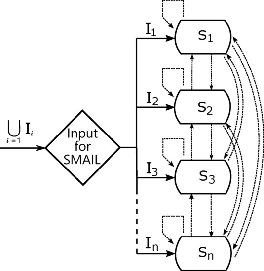
One can easily explain what is meant by Definition 6 using Figure 1. When an arbitrary input $x\in {\displaystyle \bigcup _{i=1}^n}{I}_i$ is applied, the system, i.e., the cartesian composition, has to find out in which input set x belongs. Therefore, we determine the correct line in Equation (7), which through using we obtain a new state of the system. If, for example, $x\in I_1$, the new state $s_1^{\prime }\in S_1$ will be computed. Then, it will be adjusted to $s_1^{\prime \prime }\in S_1$ using ${\phi }_{11}$, i.e., by the self-mapping internal link. This new state $s_1^{\prime \prime }\in S_1$ will be mapped to remaining input sets $I_2,I_3,\dots$ as defined by the matrix of internal links. In other words, the matrix determines which other states can be influenced by the change of the primary state. We apply inputs on states using respective transition functions. If there is 0 instead of ${\phi }_{ij}$ in the matrix of internal links, then the link between the state set $S_{ij}$ and input set $I_j$ does not exist. Notice that in Equation (7) e.g., ${\delta }_1({\phi }_{n1}\left({\delta }_n(x,s_n)\right),s_1)={\delta }_1({\phi }_{n1}\left(s^{\prime }\right),s_1)={\delta }_1(i_1,s_1)=s^{\prime \prime }$. Since we obviously have to regard directions (see the oriented arrows), the matrix of internal links is not symmetric.

In Section 3 we apply the matrix of internal links in the context of modelling the navigation of autonomous vehicles. In this context, each vehicle obviously adjusts its behaviour based on the behaviour of other vehicles. Also obviously, not all vehicles need to be autonomous, which explains the use of zeros in the matrix (only autonomous vehicles communicate).

The above reasoning can be seen applied in the following example. Notice that we will use it also for the construction of the state set in Theorems 2 and 4 of Section 3.

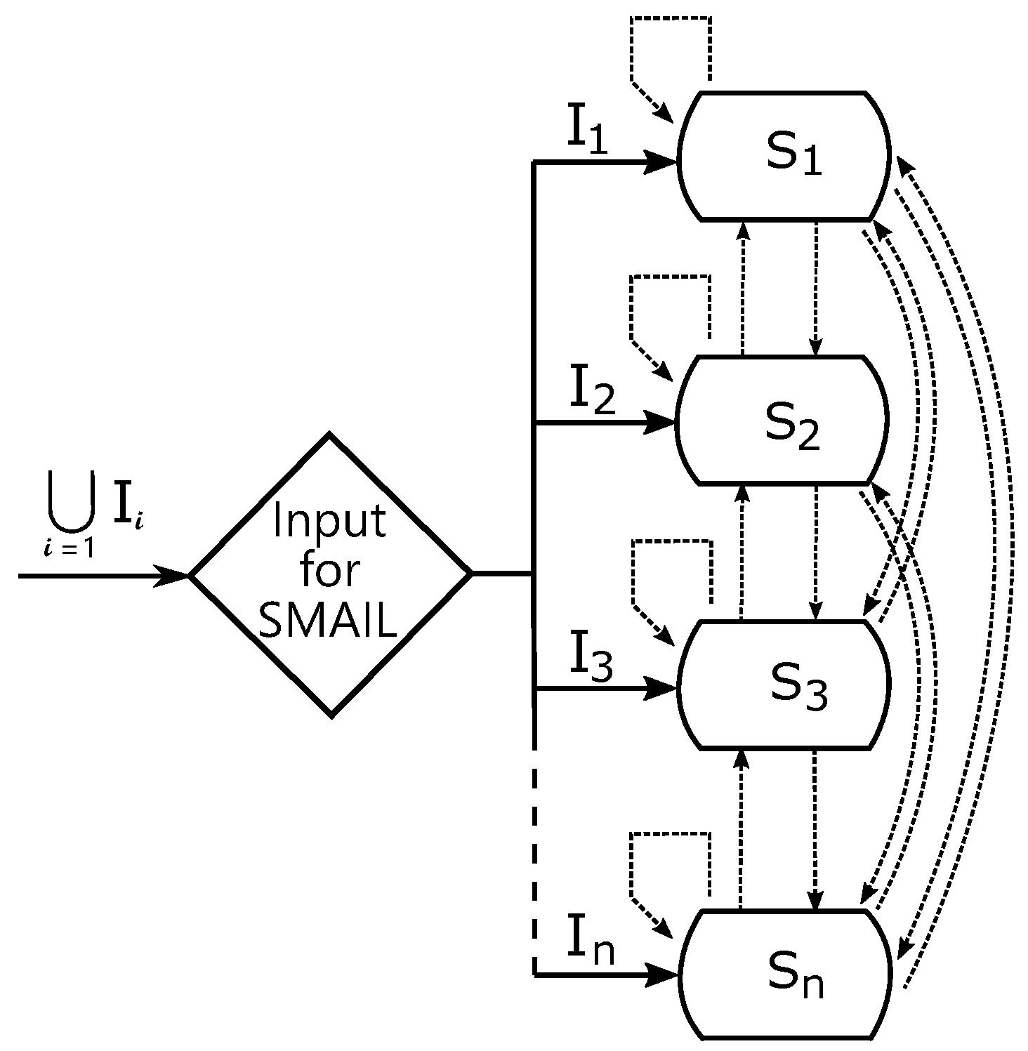
Example 1.

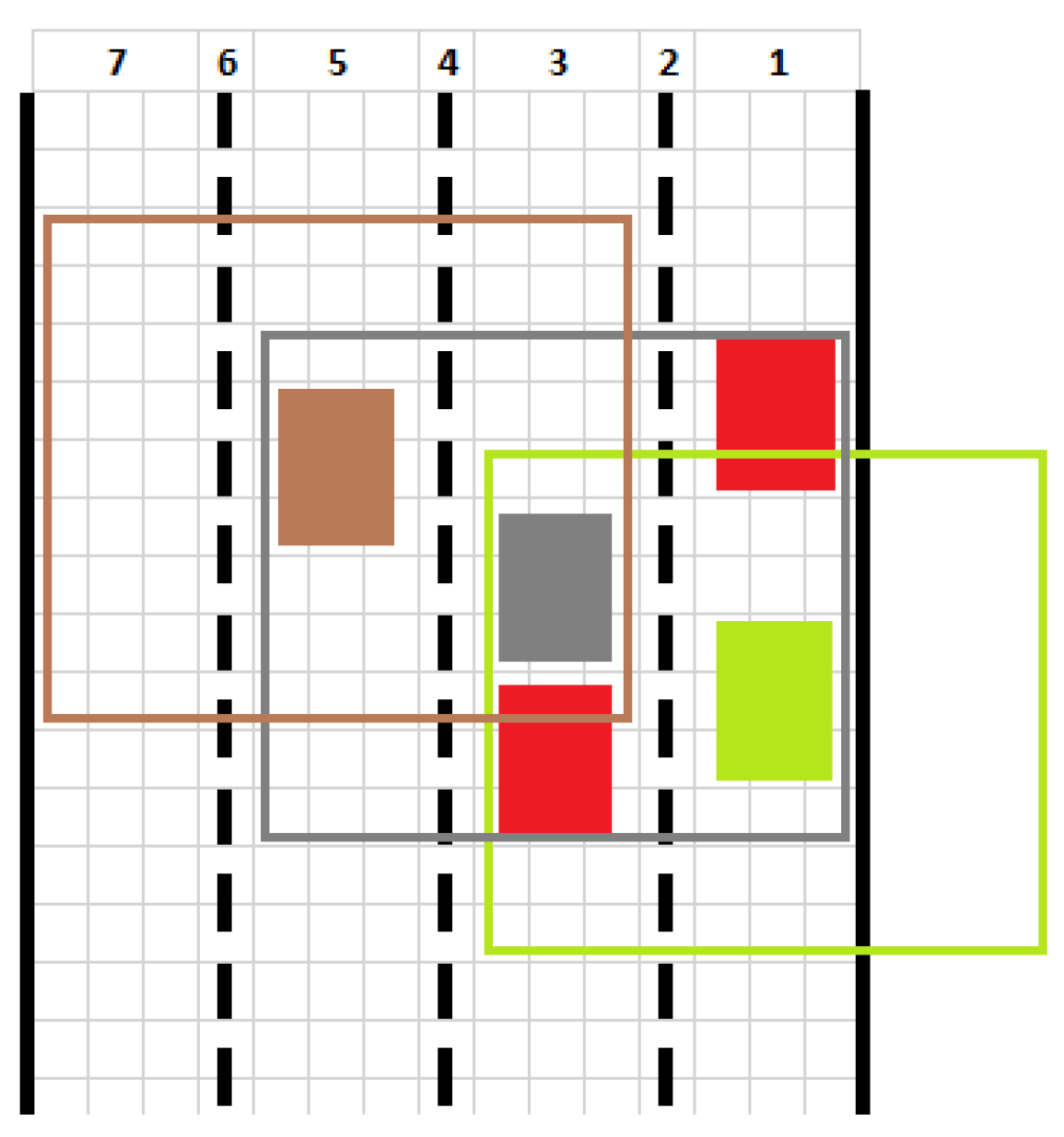
Consider a section of a road in front of an autonomously controlled intersection in Figure 2. All vehicles are autonomous with compatible self-driving control parameters. Every car is in a certain state s, for example, car $A_3$ is in state $s=\left(3;45;250;1;0;0\right)$, which means, for example, that car number 3 going at $45km/h$ is in the position $250m$ from the intersection in the 1st lane from the right. The first 0 means no change in speed while the second 0 means that the car is about to turn left.

In our system it is obvious that vehicle $A_3$ does not need to communicate with vehicle $A_4$ because it is not an obstacle in its intended driving operation. Thus, introducing an internal link between $A_3$ and $A_4$ is not necessary. However, vehicles $A_1$ and $A_2$ are problematics for $A_3$ because it intends to turn left. Therefore, $A_1$ should increase its speed while $A_2$ should slow down.

Remark 1.

Notice that some theoretical requests in the above example are not possible or even absurd, i.e., we have to keep in mind their feasibility. We already faced this problem in [12,23], where it was eliminated by using a suitable state set, input set, or operations on them. In this paper, we will choose special input and state sets as well.

3. $\mathcal{S}\mathbb{MA}il$—Application of the Theoretical Model for Autonomous Cooperation

We are going to construct our system, called $\mathcal{S}\mathbb{MA}il$, for the above context of Example 1. Naturally, Example 1 is an example of a possible usage of $\mathcal{S}\mathbb{MA}il$ only.

First, we need to define suitable sets ${\mathbb{S}}_{\mathcal{R}M}^p$ and $I_{\mathcal{VM}}^p$, where $p\in \mathbb{N}$ is the index. The elements of the state set are ordered pairs—the first component being an ordered sextuple of numbers while the second component is a matrix. The state set is

$$\begin{array}{c}\hfill {\mathbb{S}}_{\mathcal{R}M}^p=\left\{[s;\mathbf{A}],|s\in {\mathcal{R}}_6^p,\mathbf{A}\in {\mathbf{M}}_{m,n}\right\},\end{array}$$

(9)

where

$$\begin{array}{c}\hfill {\mathcal{R}}_6^p=\left\{s=(s_1,s_2,\dots s_6)|s_1=p;s_2,s_3,s_5\in {\mathbb{R}}_0^{+};s_4,\in \mathbb{N};s_6\in \langle -\frac{\pi }{4},\frac{\pi }{4}\rangle \right\}\end{array}$$

(10)

and

$$\begin{array}{c}\hfill {\mathbf{M}}_{m,n}=\left\{\left[\begin{array}{ccc}{a}_{11}& \dots & a_{1n}\\ ⋮& \ddots & ⋮\\ a_{m1}& \dots & a_{mn}\end{array}\right]|a_{ij}\in \left\{\begin{array}{cc}\left\{0\right\}\hfill & \mathrm{for}i=\frac{m+1}{2},j=\frac{n+1}{2};\hfill \\ \{-1,0,1\}\hfill & \mathrm{for}otherwise\hfill \end{array}\right.\right\}\end{array}$$

(11)

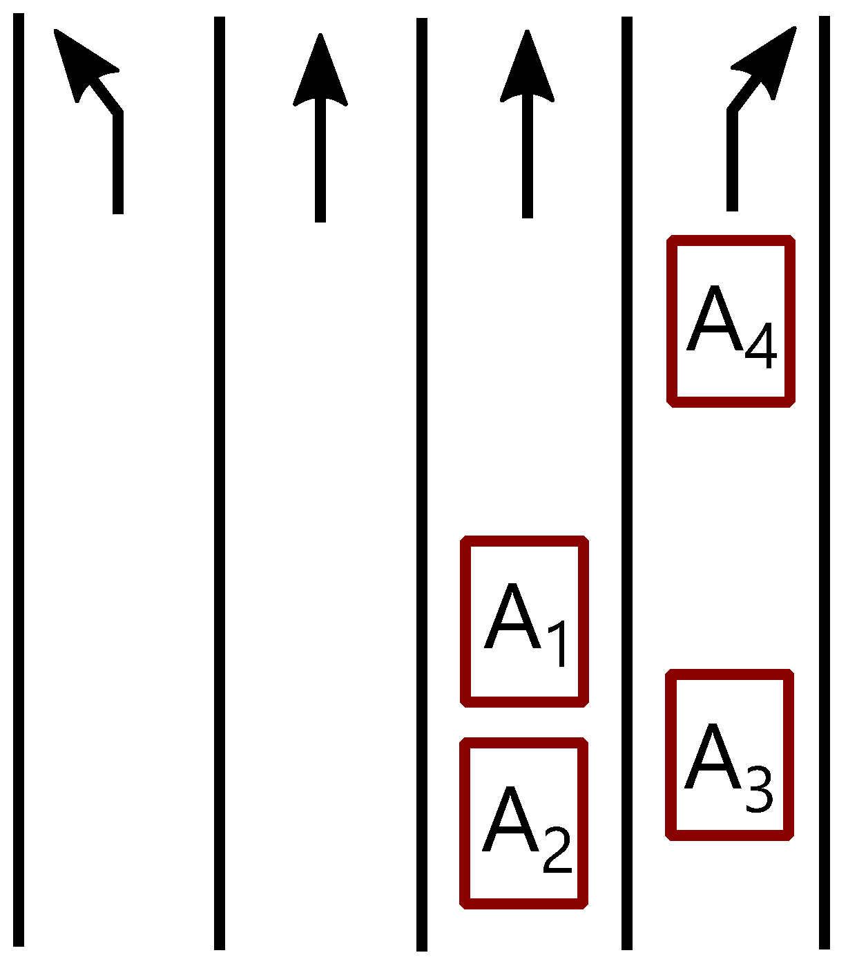
where $m,n$ are a odd numbers. The state set describes the complete position of every vehicle in all lanes. Notice that this is the same approach as in [24,25]. Now, the elements of ${\mathcal{R}}_6^p$ defined by Equation (10) correspond to states mentioned in Example 1, i.e., $s_1$ stands for the vehicle number, $s_2$ for its speed, $s_3$ for distance from the intersection, $s_4$ for the respective lane (calculated from the right using odd numbers only, even number are reserved for positions between two lanes), $s_5$ stands for changing velocity (i.e., an interval $(0,1)$ is deceleration, an interval $(1,\infty )$ is acceleration, 1 stands for constant speed), $s_6$ stands for changing direction (i.e., an interval $[-\frac{\pi }{4},0)$ means manoeuvring left, interval $(0,\frac{\pi }{4}]$ means manoeuvring right, 0 means straight direction). Of course, more parameters can be used; for an example see [26]. Matrices $\mathbf{A}$ used in Equation (9) are taken from the set ${\mathbf{M}}_{m,n}$ defined by Equation (11). Notice that we use these matrices in the form suggested in [25,27,28] where, for the purpose of its control policy, the intersection is divided into a grid of reservation tiles. To be more precise,

$$\begin{array}{c}\hfill \mathbf{A}=\left[\begin{array}{ccccccccc}\hfill -1& \hfill -1& \hfill -1& \hfill -1& \hfill -1& \hfill -1& \hfill 1& \hfill 1& \hfill 1\\ \hfill 1& \hfill 1& \hfill 1& \hfill -1& \hfill -1& \hfill -1& \hfill 1& \hfill 1& \hfill 1\\ \hfill 1& \hfill 1& \hfill 1& \hfill -1& \hfill -1& \hfill -1& \hfill -1& \hfill -1& \hfill -1\\ \hfill 1& \hfill 1& \hfill 1& \hfill -1& \hfill -1& \hfill -1& \hfill -1& \hfill -1& \hfill -1\\ \hfill -1& \hfill -1& \hfill -1& \hfill 0& \hfill 0& \hfill 0& \hfill -1& \hfill -1& \hfill -1\\ \hfill -1& \hfill -1& \hfill -1& \hfill 0& \hfill 0& \hfill 0& \hfill 1& \hfill 1& \hfill 1\\ \hfill -1& \hfill -1& \hfill -1& \hfill 0& \hfill 0& \hfill 0& \hfill 1& \hfill 1& \hfill 1\\ \hfill -1& \hfill -1& \hfill -1& \hfill -1& \hfill -1& \hfill -1& \hfill 1& \hfill 1& \hfill 1\\ \hfill -1& \hfill -1& \hfill -1& \hfill -1& \hfill -1& \hfill -1& \hfill 1& \hfill 1& \hfill 1\\ \hfill -1& \hfill -1& \hfill -1& \hfill -1& \hfill -1& \hfill -1& \hfill 1& \hfill 1& \hfill 1\\ \hfill -1& \hfill -1& \hfill -1& \hfill -1& \hfill -1& \hfill -1& \hfill -1& \hfill -1& \hfill -1\end{array}\right]\in {\mathbf{M}}_{m,n}\end{array}$$

(12)

where 0 are parts of the grid (or tiles) occupied by the given vehicle, 1 stands for tiles occupied by some other vehicles and $-1$ are free tiles. The above matrix $\mathbf{A}$ describes the situation depicted in Figure 3 from the point of view of $A_3$.

Next, for construction of the i-th quasi-multiautomaton and consequently $\mathcal{S}\mathbb{MA}il$, we will need an input alphabet, i.e., input sets (since we will be working with quasi-multiautomata, these will be algebraic hyperstructures). As mentioned above, we will define $I_{\mathcal{VM}}^p$, where $p\in \mathbb{N}$ is the index of the input set.

$$\begin{array}{c}{I}_{\mathcal{VM}}^p=\left\{\left[\overrightarrow{i},{\mathbf{C}}_{m,n}\right]=\left[(i_1,i_2,\dots ,i_6),\left[\begin{array}{ccc}{c}_{11}& \dots & c_{1n}\\ ⋮& \ddots & ⋮\\ c_{m1}& \dots & c_{mn}\end{array}\right]\right]\right.\hfill \\ |i_1=p,i_2\in {\mathbb{R}}_0^{+},i_3\in \langle 0,1\rangle ,i_4\in {\mathbb{N}}_0,i_5\in {\mathbb{R}}^{+},i_5\in 〈-\frac{\pi }{4},\frac{\pi }{4}〉,\\ \hfill \left.\phantom{\left[\begin{array}{ccc}{c}_{11}& \dots & c_{1n}\\ ⋮& \ddots & ⋮\\ c_{m1}& \dots & c_{mn}\end{array}\right]}{c}_{ij}\in \{-1,1\},i\in \{1,2,\dots ,n\},j\in \{1,2,\dots ,m\}\right\}\end{array}$$

(13)

It is obvious that input sets $I_{V,M}^p$ and $I_{V,M}^q$ are disjunct for $p\ne q$, because the first component of every vector used in $[\overrightarrow{v},{\mathbf{A}}_{n,m}]\in I_{\mathcal{VM}}^p$ is p while the first component of every vector used in $[\overrightarrow{u},{\mathbf{B}}_{n,m}]\in I_{\mathcal{VM}}^q$ is q, i.e.,

$$I_{V,M}^p\cap I_{V,M}^q=\varnothing ,\mathrm{for}\mathrm{every}p,q\in \mathbb{N},\mathrm{where}p\ne q.$$

Since vector components are real (or even natural) numbers, we can suppose that their sets are ordered; we write ≤ for this ordering. For all $p\in \mathbb{N}$ we define hyperoperation ${\ast }_p:I_{\mathcal{VM}}^p\times I_{\mathcal{VM}}^p\to {\mathcal{P}}^{\ast }\left(I_{\mathcal{VM}}^p\right)$ by:

$$\begin{array}{c}\left[\overrightarrow{u},{\mathbf{A}}_{m,n}\right]{\ast }_p\left[\overrightarrow{v},{\mathbf{B}}_{m,n}\right]=\\ \left\{\left[\overrightarrow{w},{\mathbf{C}}_{m,n}\right]\mid min\{u_i,v_i\}\le w_i\le max\{u_i,v_i\},\mathrm{for}\mathrm{every}i\in \mathbb{N},{\mathbf{C}}_{m,n}\in \{{\mathbf{A}}_{m,n},{\mathbf{B}}_{m,n}\}\right\}.\end{array}$$

(14)

In the following example we show what we mean by the hyperoperation. Notice that the hyperoperation will be later on used to construct a hypergroup in Theorem 1, which will fulfil the assumption regarding input alphabet stated in Definition 2.

Example 2.

Consider two elements $\left[\overrightarrow{a},{\mathbf{A}}_{2,3}\right],\left[\overrightarrow{c},{\mathbf{C}}_{2,3}\right]\in I_{\mathcal{VM}}^2$, where $\left[\overrightarrow{a},{\mathbf{A}}_{2,3}\right]=\left[(2;6.2;0;1;4;-\frac{\pi }{8}),\left[\begin{array}{ccc}1& -1& 1\\ 1& -1& -1\end{array}\right]\right]$ and $\left[\overrightarrow{c},{\mathbf{C}}_{2,3}\right]=\left[(2;8.1;1;2;5;\frac{\pi }{6}),\left[\begin{array}{ccc}-1& -1& -1\\ 1& -1& -1\end{array}\right]\right]$. Then the hyperoperarion

$$\begin{array}{c}\left[\overrightarrow{a},{\mathit{A}}_{2,3}\right]{\ast }_p\left[\overrightarrow{c},{\mathit{C}}_{2,3}\right]=\left[(2;6.2;0;1;4;-\frac{\pi }{8}),\left[\begin{array}{ccc}1& -1& 1\\ 1& -1& -1\end{array}\right]\right]{\ast }_p\left[(2;8.1;1;2;5;\frac{\pi }{6}),\left[\begin{array}{ccc}-1& -1& -1\\ 1& -1& -1\end{array}\right]\right]=\\ \left\{\left[(2;r_2;r_3;r_4;r_5;r_6),{\mathbf{D}}_{2,3}\right]\mid 6.2\le r_2\le 8.1;0\le r_3\le 1;1\le r_4\le 2;4\le r_5\le 5;-\frac{\pi }{8}\le r_6\le \frac{\pi }{6}\right\},\end{array}$$

where $\left[\overrightarrow{r},{\mathit{D}}_{2,3}\right]$ is defined by Equation (14), i.e., ${\mathbf{D}}_{2,3}\in \left\{\left[\begin{array}{ccc}1& -1& 1\\ 1& -1& -1\end{array}\right],\left[\begin{array}{ccc}-1& -1& -1\\ 1& -1& -1\end{array}\right]\right\}$.

Theorem 1.

For every index $p\in \mathbb{N}$, the pairs $(I_{\mathcal{VM}}^p,{\ast }_p)$ are hypergroups.

Proof. 

First, we have to show that the associativity axiom holds, i.e., for all $\left[\overrightarrow{u},{\mathbf{A}}_{m,n}\right];\left[\overrightarrow{v},{\mathbf{B}}_{m,n}\right];\left[\overrightarrow{w},{\mathbf{C}}_{m,n}\right]\in I_{\mathcal{VM}}^p$ there is $\left[\overrightarrow{u},{\mathbf{A}}_{m,n}\right]{\ast }_p\left(\left[\overrightarrow{v},{\mathbf{B}}_{m,n}\right]{\ast }_p\left[\overrightarrow{w},{\mathbf{C}}_{m,n}\right]\right)=\left(\left[\overrightarrow{u},{\mathbf{A}}_{m,n}\right]{\ast }_p\left[\overrightarrow{v},{\mathbf{B}}_{m,n}\right]\right){\ast }_p\left[\overrightarrow{w},{\mathbf{C}}_{m,n}\right]$. Without losing generality, we can show that associativity axiom holds for both matrices and vectors. First, we consider vectors:

$$\begin{array}{c}\overrightarrow{u}{\ast }_p\left(\overrightarrow{v}{\ast }_p\overrightarrow{w}\right)=\overrightarrow{u}{\ast }_p\left\{\overrightarrow{r},min\{v_i,w_i\}\le r_i\le max\{v_i,w_i\}\right\}=\\ \bigcup _{\overrightarrow{s}\in \left\{\overrightarrow{r},min\{v_i,w_i\}\le r_i\le max\{v_i,w_i\}\right\}}\overrightarrow{u}{\ast }_p\overrightarrow{s}=\bigcup _{\overrightarrow{s}\in \left\{\overrightarrow{r},min\{v_i,w_i\}\le r_i\le max\{v_i,w_i\}\right\}}\left\{\overrightarrow{t},min\{u_i,s_i\}\le t_i\le max\{u_i,s_i\}\right\}=\\ \left\{\overrightarrow{t},min\{u_i,min\{v_i,w_i\}\}\le t_i\le max\{u_i,max\{v_i,w_i\}\}\right\}=\left\{\overrightarrow{t},min\{u_i,v_i,w_i\}\le t_i\le max\{u_i,v_i,w_i\}\}\right\}=\\ \left\{\overrightarrow{t},min\{min\{u_i,v_i\},w_i\}\le t_i\le max\{min\{u_i,v_i\},w_i\}\right\}=\\ \bigcup _{\overrightarrow{a}\in \left\{\overrightarrow{b},min\{u_i,v_i\}\le b_i\le max\{u_i,v_i\}\right\}}\left\{\overrightarrow{c},min\{w_i,a_i\}\le c_i\le max\{w_i,a_i\}\right\}=\bigcup _{\overrightarrow{a}\in \left\{\overrightarrow{b},min\{u_i,v_i\}\le b_i\le max\{u_i,v_i\}\right\}}\overrightarrow{a}{\ast }_p\overrightarrow{w}=\\ \left\{\overrightarrow{b},min\{u_i,v_i\}\le b_i\le max\{u_i,v_i\}\right\}{\ast }_p\overrightarrow{w}=\left(\overrightarrow{u}{\ast }_p\overrightarrow{v}\right){\ast }_p\overrightarrow{w}.\end{array}$$

In the case of matrices, the proof is straightforward:

$$\begin{array}{c}\mathbf{A}{\ast }_p\left(\mathbf{B}{\ast }_p\mathbf{C}\right)=\mathbf{A}{\ast }_p\{\mathbf{B},\mathbf{C}\}=\mathbf{A}{\ast }_p\mathbf{B}\cup \mathbf{A}{\ast }_p\mathbf{C}=\{\mathbf{A},\mathbf{B}\}\cup \{\mathbf{A},\mathbf{C}\}=\{\mathbf{A},\mathbf{B},\mathbf{C}\}\\ =\{\mathbf{A},\mathbf{C}\}\cup \{\mathbf{B},\mathbf{C}\}=\mathbf{A}{\ast }_p\mathbf{C}\cup \mathbf{B}{\ast }_p\mathbf{C}=\{\mathbf{A},\mathbf{B}\}{\ast }_p\mathbf{C}=\left(\mathbf{A}{\ast }_p\mathbf{B}\right){\ast }_p\mathbf{C}.\end{array}$$

The reproductivity axiom holds automatically because the hyperoperation defined above is obviously extensive, i.e., for all $\mathbf{A},\mathbf{B}\in I_{\mathcal{VM}}^p$ there is $\{\mathbf{A},\mathbf{B}\}\subseteq \mathbf{A}{\ast }_p\mathbf{B}$. So for arbitrary $\left[\overrightarrow{v},{\mathbf{B}}_{m,n}\right]$ we have $\left[\overrightarrow{v},{\mathbf{B}}_{m,n}\right]\ast I_{\mathcal{VM}}^p=\bigcup _{\left[\overrightarrow{u},{\mathbf{C}}_{m,n}\right]\in I_{\mathcal{VM}}^p}\left[\overrightarrow{v},{\mathbf{B}}_{m,n}\right]\ast \left[\overrightarrow{u},{\mathbf{C}}_{m,n}\right]=I_{\mathcal{VM}}^p$. Thus, for all indices $p\in \mathbb{N}$ the structures $(I_{\mathcal{VM}}^p,{\ast }_p)$ are hypergroups. □

At this point, everything is ready for the construction of an e-quasi-multiautomaton with the state set ${\mathbb{S}}_{\mathcal{R}M}^p$ and input set $I_{\mathcal{VM}}^p$ for p-th quasi-automaton, where $p\in \mathbb{N}$.

Remark 2.

We consider ordered pairs of vectors and matrices as elements of the input set and also of the state set. As a result, we will denote elements with index ı for input and with index s for the state, i.e., $\left[\overrightarrow{a^{ı}},{\mathbf{A}}_{m,n}^{ı}\right]$ is an input word and $\left[u^s,{\mathbf{M}}_{m,n}^s\right]$ is a state.

Theorem 2.

For every index $p\in \mathbb{N}$ the triple ${\mathbb{MA}}_p=(I_{\mathcal{VM}}^p,{\mathbb{S}}_{\mathcal{R}M}^p,{\delta }_p)$ is an e-quasi-multiautomtaton with input hypergroup $(I_{\mathcal{VM}}^p,{\ast }_p)$, where transition function ${\delta }_p:I_{\mathcal{VM}}^p\times {\mathbb{S}}_{\mathcal{R}M}^p\to {\mathbb{S}}_{\mathcal{R}M}^p$ is defined by

$$\begin{array}{c}\hfill {\delta }_p\left(\left[\overrightarrow{a^{ı}},{\mathbf{C}}_{m,n}^{ı}\right],\left[v^s,{\mathbf{K}}_{m,n}^s\right]\right)=\end{array}$$

(15)

$$\begin{array}{c}\hfill \left[{\left(\sqrt{a_1·v_1};a_2·v_2+a_2;a_3·v_3;a_4+v_4\equiv mod2l-1;a_5·v_5;a_6+0·v_6\right)}_s,{\left[\begin{array}{ccc}{c}_{11}{k}_{11}& \cdots & c_{1n}{k}_{1n}\\ \cdots & \cdots & \cdots \\ c_{m1}{k}_{m1}& \cdots & c_{mn}{k}_{mn}\end{array}\right]}^s\right].\end{array}$$

Proof. 

This proof is constructed as follows: first we calculate left hand side condition E-GMAC, second we show that left hand side is included in right hand side.

The left hand side:

$$\begin{array}{c}{\delta }_p\left(\left[\overrightarrow{a^{ı}},{\mathbf{A}}_{m,n}^{ı}\right],{\delta }_p\left(\left[\overrightarrow{b^{ı}},{\mathbf{B}}_{m,n}^{ı}\right],\left[u^s,{\mathbf{U}}_{m,n}^s\right]\right)\right)=\\ {\delta }_p\left(\left[\overrightarrow{a^{ı}},{\mathbf{A}}_{m,n}^{ı}\right],\left[{\left(\sqrt{b_1{u}_1};b_2{u}_2+b_2;b_3{u}_3;b_4+u_4\equiv mod2l-1;b_5{u}_5;b_6+0·u_6\right)}_s,{\left(b_{ij}{u}_{ij}\right)}^s\right]\right)=\\ {\delta }_p\left(\left[\overrightarrow{a^{ı}},{\mathbf{A}}_{m,n}^{ı}\right],\left[{\left(\sqrt{p^2};b_2{u}_2+b_2;b_3{u}_3;b_4+u_4\equiv mod2l-1;b_5{u}_5;b_6\right)}_s,{\left(b_{ij}{u}_{ij}\right)}^s\right]\right)=\\ \left[{\left(\sqrt{a_{1}p};a_2(b_2{u}_2+b_2)+a_2;a_3{b}_3{u}_3;a_4+b_4+u_4\equiv mod2l-1;a_5{b}_5{u}_5;a_6+(0·b_6)\right)}_s,{\left(a_{ij}{b}_{ij}{u}_{ij}\right)}^s\right]=\\ \left[{\left(\sqrt{p^2};a_2(b_2{u}_2+b_2)+a_2;a_3{b}_3{u}_3;a_4+b_4+u_4\equiv mod2l-1;a_5{b}_5{u}_5;a_6\right)}_s,{\left(a_{ij}{b}_{ij}{u}_{ij}\right)}^s\right]=\\ \left[{\left(p;a_2(b_2{u}_2+b_2)+a_2;a_3{b}_3{u}_3;a_4+b_4+u_4\equiv mod2l-1;a_5{b}_5{u}_5;a_6\right)}_s,{\left(a_{ij}{b}_{ij}{u}_{ij}\right)}^s\right]=\\ \left[v^s,{\mathbf{V}}_{m,n}^s\right].\end{array}$$

The right hand side:

$$\begin{array}{c}{\delta }_p\left(\left[\overrightarrow{a^{ı}},{\mathbf{A}}_{m,n}^{ı}\right],{\ast }_p\left[\overrightarrow{b^{ı}},{\mathbf{B}}_{m,n}^{ı}\right],\left[u^s,{\mathbf{U}}_{m,n}^s\right]\right)\cup {\delta }_p\left(I_{\mathcal{VM}}^p,\left[u^s,{\mathbf{U}}_{m,n}^s\right]\right).\end{array}$$

From the definition of hyperoproduct ${\ast }_p$ in Equation (14), we simply observe that the left hand side is not included in the right part of the right hand side union. Therefore, we have to proof, that the left hand side belongs to the left part of the right hand side union. Therefore we calculate:

$$\begin{array}{c}{\delta }_p\left(I_{\mathcal{VM}}^p,\left[u^s,{\mathbf{U}}_{m,n}^s\right]\right)=\bigcup _{\left[\overrightarrow{p^{ı}},{\mathbf{P}}_{m,n}^{ı}\right]\in I_{\mathcal{VM}}^p}{\delta }_p\left(\left[\overrightarrow{p^{ı}},{\mathbf{P}}_{m,n}^{ı}\right],\left[u^s,{\mathbf{U}}_{m,n}^s\right]\right)\end{array}$$

There exist an input word $\left[\overrightarrow{c^{ı}},{\mathbf{C}}_{m,n}^{ı}\right]\in I_{\mathcal{VM}}^p$ such that the vector is $\overrightarrow{c}=\left(p;\frac{a_2{i}_{2}s+a_2{i}_2+a}{s+1};a_3{b}_3;a_4+b_4;a_5{b}_5;a_6\right)$ and the matrix is $\mathbf{C}={\left[\begin{array}{ccc}{a}_{11}{b}_{11}& \cdots & a_{1n}{b}_{1n}\\ \cdots & \cdots & \cdots \\ a_{m1}{b}_{m1}& \cdots & a_{mn}{b}_{mn}\end{array}\right]}^i$. Thus,

$$\begin{array}{c}\left[v^s,{\mathbf{V}}_{m,n}^s\right]={\delta }_p\left(\left[\overrightarrow{c^{ı}},{\mathbf{C}}_{m,n}^{ı}\right],\left[u^s,{\mathbf{U}}_{m,n}^s\right]\right)\in \bigcup _{\left[\overrightarrow{p^{ı}},{\mathbf{P}}_{m,n}^{ı}\right]\in I_{\mathcal{VM}}^p}{\delta }_p\left(\left[\overrightarrow{p^{ı}},{\mathbf{P}}_{m,n}^{ı}\right].\left[u^s,{\mathbf{U}}_{m,n}^s\right]\right),\end{array}$$

As a result, E-GMAC holds and the structure ${\mathbb{MA}}_p=(I_{\mathcal{VM}}^p,S_{V,M}^p,{\delta }_p)$ is an e-quasi-multiautomaton. □

Once Theorem 2 is proved we will show a practical application af e-quasi-multiautomata in intelligent transport systems. In the following example, the e-quasi-multiautomaton represents an autonomous vehicle. Its state is described by parameters organized into a sextuple while the matrix is used to detect its environment. This example is also linked to Example 1.

Example 3.

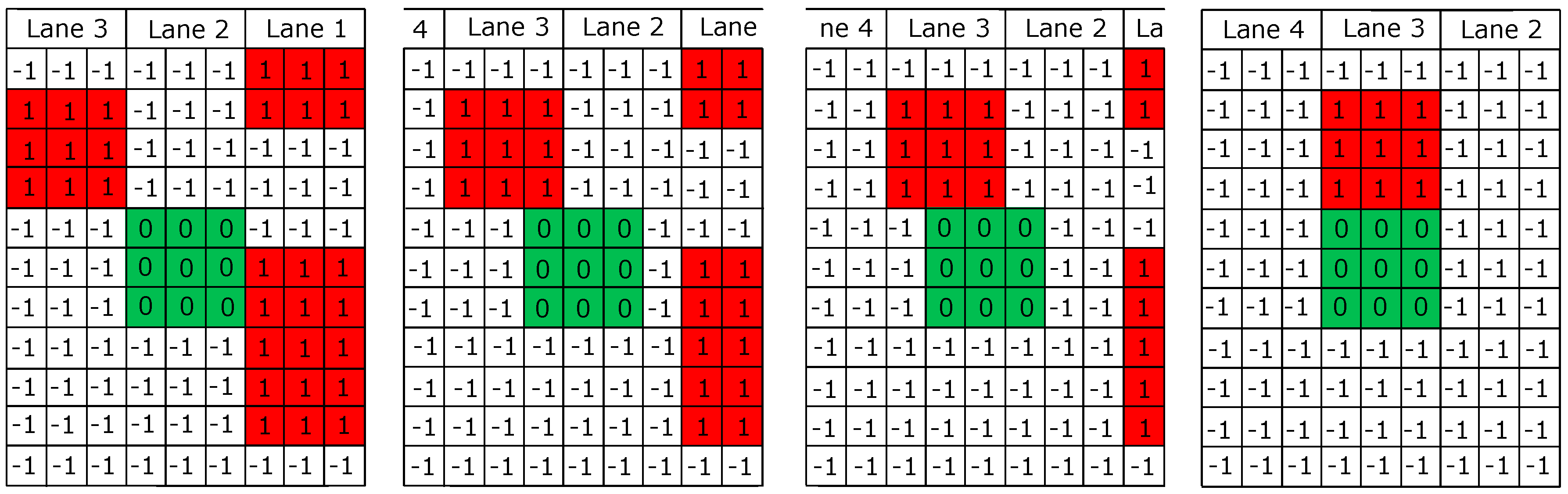
We consider matrix $\mathbf{B}$ equivalent to matrix $\mathbf{A}$ of Equation (12), which describes the situation in Figure 3. The vehicle $A_3$—in Figure 4 depicted in green (while other, non-autonomous, vehicles are red)—detects its surroundings and saves the data to matrix $\mathbf{B}$. This model is suitable for a situation where only one vehicle, such as $A_3$, is autonomous and it is not possible to establish communication with other vehicles (because they are not autonomous). We consider a state $\left[a^s,{\mathbf{B}}_{m,n}^s\right]\in S_{V,M}^3$, where ${\overrightarrow{a}}_s=(3;30;200;2;0;0)$ and values in matrix $\mathbf{B}$ corresponding to values in the first picture of Figure 4. If we apply the input $\left[\overrightarrow{s^{ı}},{\mathbf{S}}_{m,n}^{ı}\right]\in I_{\mathcal{VM}}^3$ by the transition function ${\delta }_3$, where $\overrightarrow{s^{ı}}=(3;1;0,99;1;0;-\frac{\pi }{4})$ and ${\mathbf{S}}_{m,n}^{ı}=\left[\begin{array}{ccccccccc}\hfill 1& \hfill 1& \hfill 1& \hfill 1& \hfill 1& \hfill 1& \hfill -1& \hfill 1& \hfill 1\\ \hfill -1& \hfill 1& \hfill 1& \hfill -1& \hfill 1& \hfill 1& \hfill -1& \hfill 1& \hfill 1\\ \hfill -1& \hfill 1& \hfill 1& \hfill -1& \hfill 1& \hfill 1& \hfill 1& \hfill 1& \hfill 1\\ \hfill -1& \hfill 1& \hfill 1& \hfill -1& \hfill 1& \hfill 1& \hfill 1& \hfill 1& \hfill 1\\ \hfill 1& \hfill 1& \hfill 1& \hfill 1& \hfill 1& \hfill 1& \hfill 1& \hfill 1& \hfill 1\\ \hfill 1& \hfill 1& \hfill 1& \hfill 1& \hfill 1& \hfill 1& \hfill -1& \hfill 1& \hfill 1\\ \hfill 1& \hfill 1& \hfill 1& \hfill 1& \hfill 1& \hfill 1& \hfill -1& \hfill 1& \hfill 1\\ \hfill 1& \hfill 1& \hfill 1& \hfill 1& \hfill 1& \hfill 1& \hfill -1& \hfill 1& \hfill 1\\ \hfill 1& \hfill 1& \hfill 1& \hfill 1& \hfill 1& \hfill 1& \hfill -1& \hfill 1& \hfill 1\\ \hfill 1& \hfill 1& \hfill 1& \hfill 1& \hfill 1& \hfill 1& \hfill -1& \hfill 1& \hfill 1\\ \hfill 1& \hfill 1& \hfill 1& \hfill 1& \hfill 1& \hfill 1& \hfill -1& \hfill 1& \hfill 1\end{array}\right]$, then the first component of the input word is used to control the direction, i.e., it changes the state of the sextuple. The second component of the input word changes the matrix that detects the surroundings of a vehicle. This way we obtain a new state $\left[r^s,{\mathbf{R}}_{m,n}^s\right]$, where ${\overrightarrow{s}}_i=(3;30;198;3;0;-\frac{\pi }{4})$ and the entries of the matrix ${\mathbf{R}}_{m,n}^s$ are $-\mathbf{1}$ for $a_{21},a_{24},a_{31},a_{34},a_{41},a_{44},a_{17},a_{27},a_{67},a_{77},a_{87},a_{97},a_{10,7}$ and $\mathbf{1}$ for other cases.

We know from the new state $\left[r^s,{\mathbf{R}}_{m,n}^s\right]$ that the vehicle $A_3$ does not change its velocity or its acceleration. We also know that the vehicle $A_3$ is positioned about 2$m$ far from the intersection border and is between lane 2 and 3, and it turns to the left. We can see the position surroundings in Figure 4. Consequently, this is what we use in the next step as input for full inclusion in lane 3.

We will use the e-quasi-multiautomata from Theorem 2 for the construction of a system called $\mathcal{S}\mathbb{MA}il$. Necessarily, a change on any component of the state of the system must trigger a change on another component of the state. However, there may be situations where the change of other components are not necessarily required. Therefore, we include the following theorem in which we assert that there are such inputs for which the state of the multiautomata do not change.

Theorem 3.

For every e-quasi-mulltiautomaton ${\mathbb{MA}}_p=(I_{\mathcal{VM}}^p,{\mathbb{S}}_{\mathcal{R}M}^p,{\delta }_p)$ there is an input $\left[\overrightarrow{e^{ı}},{\mathbf{E}}_{m,n}^{ı}\right]$ for which holds

$$\begin{array}{c}\hfill {\delta }_p\left(\left[\overrightarrow{e^{ı}},{\mathbf{E}}_{m,n}^{ı}\right],\left[s^s,{\mathbf{S}}_{m,n}^s\right]\right)=\left[s^s,{\mathbf{S}}_{m,n}^s\right].\end{array}$$

(16)

Proof. 

Consider an arbitrary state $\left[s^s,{\mathbf{S}}_{m,n}^s\right]\in {\mathbb{S}}_{\mathcal{R}M}^p$ of the e-quasi-mulltiautomaton ${\mathbb{MA}}_p$. For input words $\left[\overrightarrow{e^{ı}},{\mathbf{E}}_{m,n}^{ı}\right]=\left[(e_1;e_2;e_3;e_4;e_5;e_6),{\left[\begin{array}{ccc}{1}_{11}& \cdots & 1_{1n}\\ \cdots & \cdots & \cdots \\ 1_{m1}& \cdots & 1_{mn}\end{array}\right]}^i\right]$, where $e_1=p;e_2=\frac{s_2}{s_2+1};e_3=1;e_4=0;e_5=1;e_6=s_6$, there holds Equation (16). Indeed,

$$\begin{array}{c}{\delta }_p\left(\left[\overrightarrow{e^{ı}},{\mathbf{E}}_{m,n}^{ı}\right],\left[s^s,{\mathbf{S}}_{m,n}^s\right]\right)=\\ {\delta }_p\left(\left[{(p;\frac{s_2}{s_2+1};1;0;1;s_6)}_i,{\left[\begin{array}{ccc}{1}_{11}& \cdots & 1_{1n}\\ \cdots & \cdots & \cdots \\ 1_{m1}& \cdots & 1_{mn}\end{array}\right]}^i\right],\left[{(s_1;s_2;s_3;s_4;s_5;s_6)}_s,{\left[\begin{array}{ccc}{a}_{11}& \cdots & a_{1n}\\ \cdots & \cdots & \cdots \\ a_{m1}& \cdots & a_{mn}\end{array}\right]}^s\right]\right)=\\ \left[\left(\sqrt{p^2},\frac{s_2}{s_2+1}{s}_2+\frac{s_2}{s_2+1},1·s_3,0+s_4\equiv modk-1,1·s_5,s_6+0·s_6\right){\left[\begin{array}{ccc}{1}_{11}{a}_{11}& \cdots & 1_{1n}{a}_{1n}\\ \cdots & \cdots & \cdots \\ 1_{m1}{a}_{m1}& \cdots & 1_{mn}{a}_{mn}\end{array}\right]}^s\right]=\\ \left[\left(p,\frac{s_2(s_2+1)}{s_2+1}{s}_3,s_4,s_5,s_6\right),{\left[\begin{array}{ccc}{a}_{11}& \cdots & a_{1n}\\ \cdots & \cdots & \cdots \\ a_{m1}& \cdots & a_{mn}\end{array}\right]}^s\right]=\left[s^s,{\mathbf{S}}_{m,n}^s\right]\end{array}$$

□

In Example 4 we consider different e-quasi-multiautomata as parts of a cooperative intelligent transport system. Some e-quasi-multiautomata represent autonomous vehicles while some are non-autonomous vehicles. Obviously, non-autonomous vehicles cannot detect their surroundings. In such cases we will use e-quasi-multiautomata, in which all entries of state matrices are 0. This explains the inclusion of the following lemma.

Lemma 1.

Let ${\overline{{\mathbb{S}}^p}}_{\mathcal{R}M}=\left\{[s;\mathbf{A}]|s\in {\mathcal{R}}_6^p,a_{ij}=0\right\},$ then a structure $sub{\mathbb{MA}}_p=(I_{\mathcal{VM}}^p,{\overline{{\mathbb{S}}^p}}_{\mathcal{R}M},{\delta }_p)$ is a sub-e-quasi-multiautomaton of e-quai-multiautomaton ${\mathbb{MA}}_p=(I_{\mathcal{VM}}^p,{\mathbb{S}}_{\mathcal{R}M}^p,{\delta }_p)$.

Proof. 

It is obvious that ${\overline{{\mathbb{S}}^p}}_{\mathcal{R}M}\subset {\mathbb{S}}_{\mathcal{R}M}^p$ and ${\delta }_p:I_{\mathcal{VM}}^p\times {\overline{{\mathbb{S}}^p}}_{\mathcal{R}M}\to {\overline{{\mathbb{S}}^p}}_{\mathcal{R}M}$. Next, we can see that E-GMAC holds because all entries in the state matrix are zero. Thus, the second component of the state can not change for any input. Therefore, the proof for the first component is the same as the proof of the Theorem 2. □

In what follows, we will note that every state $\left[{}_p{s}^s,{}_p{\mathbf{S}}_{m,n}^s\right]$ is equal to $\left[\left({}_p{s}_1^s,\dots {,}_p{s}_6^s\right){,}_p{b}_{ij}^s\right]\in {\mathbb{S}}_{\mathcal{R}M}^p$ and every input $\left[{}_p\overrightarrow{a^{ı}}{,}_p{\mathbf{A}}_{m,n}^{ı}\right]$ is equal to $\left[\left({}_p{a}_1^{ı},\dots {,}_p{a}_6^{ı}\right){,}_p{a}_{ij}^{ı}\right]\in I_{\mathcal{VM}}^p$ from e-quasi-multiautomaton ${\mathbb{MA}}_p=(I_{\mathcal{VM}}^p,{\mathbb{S}}_{\mathcal{R}M}^p,{\delta }_p)$, where $p\in \mathbb{N}$ is an index. In the other words, such as ${}_p{s}_1^s$, the upper index s denotes state element, lower index 1 denotes position in the sextuple and the lower index p denotes the $p-th$ e-quasi-multiautomaton. The indices in matrices have the same meaning. As far as input words are regarded, we use upper index ı; other indices have the same meaning.

Now we need to define the matrix of internal links. First, we define ${\phi }_{pp}:{\mathbb{S}}_{\mathcal{R}M}^p\to I_{\mathcal{VM}}^p$ for all $p\in \{1,2,\dots ,n\}$ by

$$\begin{array}{c}\hfill {\phi }_{pp}\left(\left[{(}_p{s}_1^s{,}_p{s}_2^s{,}_p{s}_3^s{,}_p{s}_4^s{,}_p{s}_5^s{,}_p{s}_6^s){,}_p{\mathbf{A}}_{m,n}^s\right]\right)=\left[{(}_p{v}_1^{ı}{,}_p{v}_2^{ı}{,}_p{v}_3^{ı}{,}_p{v}_4^{ı}{,}_p{v}_5^{ı}{,}_p{v}_6^{ı}){,}_p{\mathbf{B}}_{m,n}^{ı}\right].\end{array}$$

where ${}_p{v}_1^{ı}={}_p{s}_1^s=p;{}_p{v}_2^{ı}=\frac{{}_p{s}_2^s}{{}_p{s}_2^s+\frac{1}{{}_p{s}_5^s}};{}_p{v}_3^{ı}=0,95;{}_p{v}_4^{ı}={}_p{s}_4^s+l+sgn\left(s_6^s\right);{}_p{v}_5^{ı}=\frac{1}{{}_p{s}_5^s};{}_p{v}_6^{ı}=0$ and entries of the input matrix are dependent on the occupancy of the tiles.

Corollary 1.

For mapping ${\phi }_{pp}$ added to every e-quasi-multiautomaton ${\mathbb{MA}}_p=(I_{\mathcal{VM}}^p,{\mathbb{S}}_{\mathcal{R}M}^p,{\delta }_p)$ from Theorem 2 there holds the condition E-GMAC.

Proof. 

The proof is obvious. On the left hand side we have up to four changes of the original state in the E-GMAC condition (two inputs and two applications of the internal link). However, we have a suitable input for the right hand side, similar to the proof of Theorem 2. □

Now we will define a mapping for two different e-quasi-multiautomata, i.e., from the state set of the pth e-quasi-multiautomaton to the input set of the qth e-quasi-multiautomaton. We define mapping ${\phi }_{pq}:{\mathbb{S}}_{\mathcal{R}M}^p\to I_{\mathcal{VM}}^q$ for all $p,q\in \{1,2,\dots ,n\}$, where $p\ne q$ between two e-quai-multiautomata ${\mathbb{MA}}_p=\left((I_{\mathcal{VM}}^p,{\mathbb{S}}_{\mathcal{R}M}^p,{\delta }_p)\right)$ and ${\mathbb{MA}}_q=\left((I_{\mathcal{VM}}^q,{\mathbb{S}}_{\mathcal{R}M}^q,{\delta }_q)\right)$ by

$$\begin{array}{c}\hfill {\phi }_{pq}\left(\left[{(}_p{s}_1^s,{}_p{s}_2^s,{}_p{s}_3^s,{}_p{s}_4^s,{}_p{s}_5^s,{}_p{s}_6^s){,}_p{\mathbf{A}}_{n,m}^s\right]\right)=\left[{(}_q{v}_1^{ı},{}_q{v}_2^{ı},{}_q{v}_3^{ı},{}_q{v}_4^{ı},{}_q{v}_5^{ı},{}_q{v}_6^{ı}){,}_q{\mathbf{B}}_{n,m}^{ı}\right],\end{array}$$

(17)

where

$${}_q{v}_1^{ı}=q\ne {}_p{s}_1^s;{}_q{v}_2^{ı}=\frac{{}_p{s}_2^s}{{}_p{s}_2^s+1}+\alpha {}_p{s}_5^s+\lambda ·\frac{{|}_p{s}_6^s|}{10};{}_q{v}_3^{ı}=0,99;{}_q{v}_4^{ı}=0{;}_q{v}_5^{ı}=1{;}_q{v}_6^{ı}=0.$$

Next we add a meaning of the parameters $\lambda$ and $\alpha$

$$\begin{array}{c}\hfill \lambda =\left\{\begin{array}{cc}1\hfill & {\mathrm{if}}_p{s}_4^s{>}_q{s}_4^s{\mathrm{and}}_p{s}_6^s>0\hfill \\ 1\hfill & {\mathrm{if}}_p{s}_4^s{<}_q{s}_4^s{\mathrm{and}}_p{s}_6^s<0\hfill \\ 0\hfill & otherewise\hfill \end{array}\right.\mathrm{and}\alpha =\left\{\begin{array}{cc}1\hfill & {\mathrm{if}}_p{s}_4^s{=}_q{s}_4^s\mathrm{and}q{s}_3^s{<}_p{s}_4^s{\mathrm{and}}_p{s}_5^s>1\hfill \\ 0\hfill & otherewise\hfill \end{array}\right.\end{array}$$

At this point we can give the main theorem of this section in which we are going to use all results obtained above, i.e., e-quasi-multiautomata, hypergroups, and internal links. By Definition 6 we obtain the n-ary cartesian composition of e-quasi-multiautomata with internal links.

Theorem 4.

Let ${\mathbb{MA}}_1=(I_{\mathcal{VM}}^1,{\mathbb{S}}_{\mathcal{R}M}^1,{\delta }_1),{\mathbb{MA}}_2=\left((I_{\mathcal{VM}}^2,{\mathbb{S}}_{\mathcal{R}M}^2,{\delta }_2)\right),\dots ;{\mathbb{MA}}_p=\left((I_{\mathcal{VM}}^p,{\mathbb{S}}_{\mathcal{R}M}^p,{\delta }_p)\right)$ be an e-quasi-multiautomata with disjoint input-sets $I_{\mathcal{VM}}^p$, and $p\ge 2$. Then a quadruple

$$\mathcal{S}\mathbb{MA}il=\left(\left(\bigcup _{i=1}^p{I}_{\mathcal{VM}}^i,\diamond \right),\underset{i=1}{\overset{p}{⨂}}{\mathbb{S}}_{\mathcal{R}M}^i,\prod _{i=1}^p{\delta }_i,{\mathbf{M}}_{nn}\left(\phi \right)\right)$$

is a system of the cartesian composition of e-quasi-multiautomata with internal links.

Proof. 

We have to demonstrate that the condition E-GMAC holds, i.e., that there is

$$\begin{array}{c}{\displaystyle \left(\prod _{i=1}^p{\delta }_i\right)\left(\left[\overrightarrow{a^{ı}},{\mathbf{A}}_{m,n}^{ı}\right],\left(\prod _{i=1}^p{\delta }_i\right)\left(\left[\overrightarrow{b^{ı}},{\mathbf{B}}_{m,n}^{ı}\right],\underset{i=1}{\overset{p}{⨂}}\left[{}_i{s}^s,{}_i{\mathbf{S}}_{m,n}^s\right]\right)\right)\in }\hfill \\ \hfill \left(\prod _{i=1}^p{\delta }_i\right)\left(\left[\overrightarrow{a^{ı}},{\mathbf{A}}_{m,n}^{ı}\right]{\ast }_p\left[\overrightarrow{b^{ı}},{\mathbf{B}}_{m,n}^{ı}\right],\underset{i=1}{\overset{p}{⨂}}\left[{}_i{s}^s,{}_i{\mathbf{S}}_{m,n}^s\right]\right)\cup \underset{i=1}{\overset{p}{⨂}}{\delta }_i\left(I_{\mathcal{VM}}^i,\left[{}_i{s}^s,{}_i{\mathbf{S}}_{m,n}^s\right]\right).\end{array}$$

(18)

We prove, while maintaining generality, that

$$\left(\prod _{i=1}^t{\delta }_i\right)\left(\left[\overrightarrow{a^{ı}},{\mathbf{A}}_{m,n}^{ı}\right],\left(\prod _{i=1}^t{\delta }_i\right)\left(\left[\overrightarrow{b^{ı}},{\mathbf{B}}_{m,n}^{ı}\right],\underset{i=1}{\overset{t}{⨂}}\left[{}_i{s}^s,{}_i{\mathbf{S}}_{m,n}^s\right]\right)\right)\in \underset{i=1}{\overset{t}{⨂}}{\delta }_i\left(I_{\mathcal{VM}}^i,\left[{}_i{s}^s,{}_i{\mathbf{S}}_{m,n}^s\right]\right),$$

(19)

i.e., Formula (18) without the left part of the right hand side of E-GMAC. There are two cases. The first, both input words are in the same input set, and the second, input words are from different input sets.

(a)

For the first case, we consider $\left[{}_p\overrightarrow{a^{ı}}{,}_p{\mathbf{A}}_{m,n}^{ı}\right],\left[{}_p\overrightarrow{b^{ı}}{,}_p{\mathbf{B}}_{m,n}^{ı}\right]\in I_{\mathcal{VM}}^p$. On the left hand of Equation (19), we know that the input $\left[{}_p\overrightarrow{b^{ı}}{,}_p{\mathbf{B}}_{m,n}^{ı}\right]$ works upon one component from $\left(\left[{}_1{s}^s,{}_1{\mathbf{S}}_{m,n}^s\right],\left[{}_2{s}^s,{}_2{\mathbf{S}}_{m,n}^s\right],\dots ,\left[{}_t{s}^s,{}_t{\mathbf{S}}_{m,n}^s\right]\right)$ and the state can alter by the internal link ${\phi }_{pp}$. This is performed again for input $\left[{}_p\overrightarrow{a^{ı}}{,}_p{\mathbf{A}}_{m,n}^{ı}\right]$, then we have an input $\left[{}_p\overrightarrow{c^{ı}}{,}_p{\mathbf{C}}_{m,n}^{ı}\right]\in I_{\mathcal{VM}}^p$ for which holds following (considering the proof of Theorem 2):

$${\delta }_p(\left[{}_p\overrightarrow{a^{ı}}{,}_p{\mathbf{A}}_{m,n}^{ı}\right],{\delta }_p(\left[{}_p\overrightarrow{b^{ı}}{,}_p{\mathbf{B}}_{m,n}^{ı}\right],\left[{}_p{s}^s,{}_p{\mathbf{S}}_{m,n}^s\right]))={\delta }_p(\left[{}_p\overrightarrow{c^{ı}}{,}_p{\mathbf{C}}_{m,n}^{ı}\right],\left[{}_p{s}^s,{}_p{\mathbf{S}}_{m,n}^s\right]).$$

When the inputs $\left[{}_p\overrightarrow{a^{ı}}{,}_p{\mathbf{A}}_{m,n}^{ı}\right]$ or $\left[{}_p\overrightarrow{b^{ı}}{,}_p{\mathbf{B}}_{m,n}^{ı}\right]$ are applied on the state $\left[{}_t{s}^s,{}_t{\mathbf{S}}_{m,n}^s\right]$ other states react to this change by mapping ${\phi }_{pq}$. It is obvious that mapping ${\phi }_{pr}$ influences other states by the input from the respective input set. Then for every component of the state on the right side there exists an element from the corresponding input set, that state on the left hand side is included on the right hand side.

(b)

For the second case, we consider different inputs $\left[{}_p\overrightarrow{a^{ı}}{,}_p{\mathbf{A}}_{m,n}^{ı}\right]\in I_{\mathcal{VM}}^p,\left[{}_q\overrightarrow{b^{ı}}{,}_q{\mathbf{B}}_{m,n}^{ı}\right]\in I_{\mathcal{VM}}^q$ now. On the left-hand side, we have an influence on two different components in the tuple $\left(\left[{}_1{s}^s,{}_1{\mathbf{S}}_{m,n}^s\right],\left[{}_2{s}^s,{}_2{\mathbf{S}}_{m,n}^s\right],\dots ,\left[{}_t{s}^s,{}_t{\mathbf{S}}_{m,n}^s\right]\right)$ it is evident that the same inputs are the same on the right-hand side if internal links ${\phi }_{pp}$, ${\phi }_{qq}$ do not change. At the moment, ${\phi }_{pp}$, ${\phi }_{pp}$ influence corresponding components of the state, we have suitable inputs on the right-hand side, as in proof of Theorem 2. For mapping the influence of ${\phi }_{pr}$ and ${\phi }_{qs}$ on other components, we have the same situation as case a). Thus, it is obvious that $\mathcal{S}\mathbb{MA}il$ holds condition E-GMAC.

□

In the conclusion of this section, we will demonstrate the theory explained by using the example of $\mathcal{S}\mathbb{MA}il$ to describe and model a situation with several autonomous vehicles in traffic lanes each intending to perform some action.

Example 4.

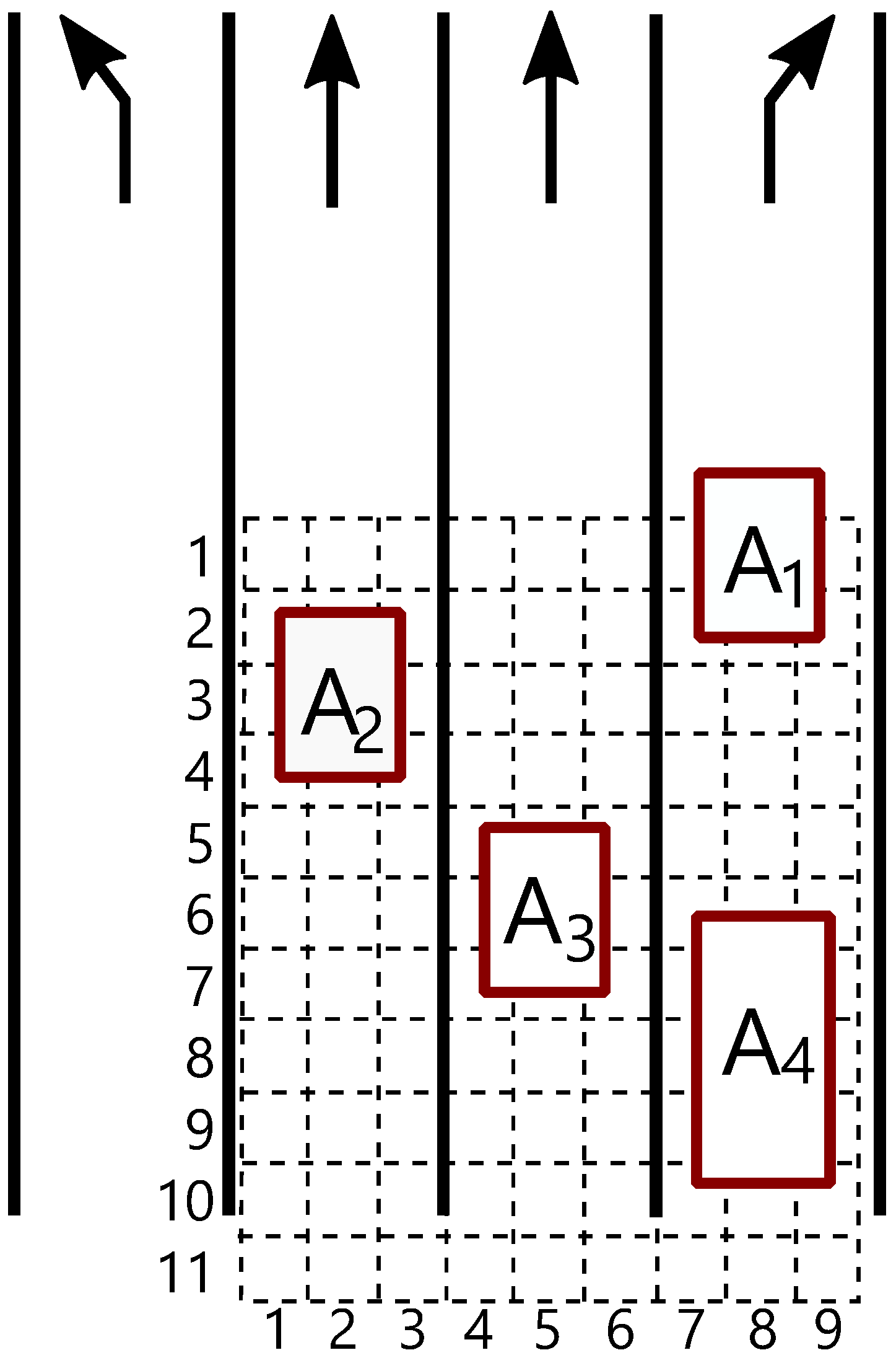
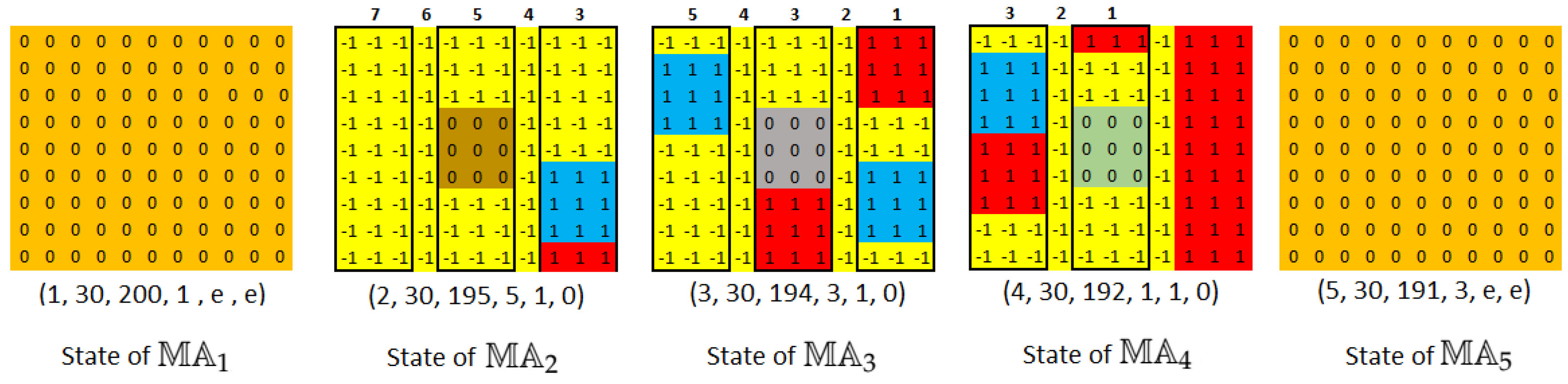
We will consider five e-quasi-multiautomata ${\mathbb{MA}}_1=(I_{\mathcal{VM}}^1,{\mathbb{S}}_{\mathcal{R}M}^1,{\delta }_1),{\mathbb{MA}}_2=(I_{\mathcal{VM}}^2,{\mathbb{S}}_{\mathcal{R}M}^2,{\delta }_2),{\mathbb{MA}}_3=(I_{\mathcal{VM}}^3,{\mathbb{S}}_{\mathcal{R}M}^3,{\delta }_3),{\mathbb{MA}}_4=(I_{\mathcal{VM}}^4,{\mathbb{S}}_{\mathcal{R}M}^4,{\delta }_4),{\mathbb{MA}}_5=(I_{\mathcal{VM}}^5,{\mathbb{S}}_{\mathcal{R}M}^5,{\delta }_5)$, where every e-quasi-multiautomaton represents a vehicle. The e-quasi-multiautomata ${\mathbb{MA}}_2,{\mathbb{MA}}_3,{\mathbb{MA}}_4$ are autonomous vehicles and ${\mathbb{MA}}_1,{\mathbb{MA}}_5$ are ordinary vehicles. Figure 5 depicts the state of every vehicle, where the vehicles ${\mathbb{MA}}_1,{\mathbb{MA}}_5$ are denoted in red colour in the same as verge of the road and other colour are used for autonomous vehicles. The complete situation with detection field of each vehicle is presented in Figure 6. In fact, Figure 5 is state of $\mathcal{S}\mathbb{MA}il$, i.e.,

$$\left(\left[{}_1{r}^s,{}_1{\mathit{R}}_{m,n}^s\right],\left[{}_2{s}^s,{}_2{\mathit{S}}_{m,n}^s\right],\left[{}_3{t}^s,{}_3{\mathit{T}}_{m,n}^s\right],\left[{}_4{u}^s,{}_4{\mathit{U}}_{m,n}^s\right],\left[{}_5{v}^s,{}_5{\mathit{V}}_{m,n}^s\right]\right).$$

Next, we need a matrix of the internal link

$$\left[\begin{array}{ccccc}0& 0& 0& 0& 0\\ 0& \phi & \phi & \phi & 0\\ 0& \phi & \phi & \phi & 0\\ 0& \phi & \phi & \phi & 0\\ 0& 0& 0& 0& 0\end{array}\right],$$

where 0 means no internal link and φ mean internal link between vehicles given by the respective indices. We are going to describe how to proceed, i.e., what input symbols to use, if the grey car, represented by e-quasi-multiautomaton ${\mathbb{MA}}_3$, wants to change lane and turn left to lane 5.

We have two approaches to start changing the lane: we can correct of the state of the vehicle directly by the component on the 2nd, 3rd and 4th position in the input word, or to use the internal link and 6th component of the input. We will use an input $\left[{(}_3{3}^{ı},{}_3{1}^{ı},{}_3{0.98}^{ı},{}_3{0}^{ı},{}_3{1}^{ı},{}_3{\frac{\pi }{5}}^{ı}),{}_3{\left(b_{i,j}\right)}^{ı}=1\right]\in I_{\mathcal{VM}}^3$, which will operate on the 6th component. Then, the resulting state—full correction—will be made by the internal link. The calculation will be done according to Equations (7) and (15), i.e.,

$$\begin{array}{c}{\delta }_3\left(\left[{(}_3{3}^{ı},{}_3{1}^{ı},{}_3{0.99}^{ı},{}_3{0}^{ı},{}_3{1}^{ı},{}_3{\frac{\pi }{5}}^{ı}),{}_3{\left(b_{i,j}\right)}^{ı}=1\right],\left[{}_3{t}^s,{}_3{\mathbf{T}}_{m,n}^s\right]\right)=\hfill \\ \hfill \left[\left({}_{3}3,{}_{3}30,{}_{3}192.06,{}_{3}3,{}_{3}1,{}_3\frac{\pi }{5}\right){,}_3{\mathbf{T}}_{n,m}^s\right]\end{array}$$

(20)

We obtain a state with new elements on the $5^{th},6$th positions where these components have an effect on other components by means of the internal link ${\phi }_{33}$ between the state and input of the e-quasi-multiautomaton ${\mathbb{MA}}_3$. With this internal link, we obtain a new input:

$${\phi }_{33}\left(\left[\left({}_3{3}^s,{}_3{30}^s,{}_3{192.06}^s,{}_3{3}^s,{}_3{1}^s,{}_3{\frac{\pi }{5}}^s\right){,}_3{\mathbf{T}}_{n,m}^s\right]\right)=\left[\left({}_3{3}^{ı},{}_3{1}^{ı},{}_3{1}^{ı},{}_3{1}^{ı},{}_3{1}^{ı},{}_3{0}^s\right){,}_3{\mathbf{C}}_{n,m}^{ı}\right],$$

where ${}_3{\mathbf{C}}_{n,m}^{ı}=\left[\begin{array}{ccccccccccc}\hfill 1& \hfill 1& \hfill 1& \hfill 1& \hfill 1& \hfill 1& \hfill 1& \hfill 1& \hfill 1& \hfill 1& \hfill -1\\ \hfill -1& \hfill 1& \hfill 1& \hfill -1& \hfill 1& \hfill 1& \hfill 1& \hfill 1& \hfill 1& \hfill 1& \hfill -1\\ \hfill -1& \hfill 1& \hfill 1& \hfill -1& \hfill 1& \hfill 1& \hfill 1& \hfill 1& \hfill 1& \hfill 1& \hfill -1\\ \hfill -1& \hfill 1& \hfill 1& \hfill -1& \hfill 1& \hfill 1& \hfill 1& \hfill 1& \hfill 1& \hfill 1& \hfill 1\\ \hfill 1& \hfill 1& \hfill 1& \hfill 1& \hfill 1& \hfill 1& \hfill 1& \hfill 1& \hfill 1& \hfill 1& \hfill 1\\ \hfill 1& \hfill 1& \hfill 1& \hfill 1& \hfill 1& \hfill 1& \hfill 1& \hfill 1& \hfill 1& \hfill 1& \hfill 1\\ \hfill 1& \hfill 1& \hfill 1& \hfill 1& \hfill 1& \hfill 1& \hfill 1& \hfill 1& \hfill 1& \hfill 1& \hfill 1\\ \hfill 1& \hfill 1& \hfill 1& \hfill 1& \hfill 1& \hfill 1& \hfill 1& \hfill 1& \hfill 1& \hfill 1& \hfill 1\\ \hfill 1& \hfill 1& \hfill 1& \hfill 1& \hfill -1& \hfill 1& \hfill 1& \hfill -1& \hfill 1& \hfill 1& \hfill -1\\ \hfill 1& \hfill 1& \hfill 1& \hfill 1& \hfill -1& \hfill 1& \hfill 1& \hfill -1& \hfill 1& \hfill 1& \hfill -1\\ \hfill 1& \hfill 1& \hfill 1& \hfill 1& \hfill -1& \hfill 1& \hfill 1& \hfill -1& \hfill 1& \hfill 1& \hfill -1\end{array}\right]$, i.e., matrix to correct the state matrix detecting other vehicles or obstacles near vehicle $A_3$.

When we apply a new input on the state $\left[\left({}_{3}3,{}_{3}30,{}_{3}192.06,{}_{3}3,{}_{3}1,{}_3\frac{\pi }{5}\right){,}_3{\mathbf{T}}_{n,m}^s\right]$, we obtain

$${\delta }_3\left(\left[{(}_3{3}^{ı},{}_3{1}^{ı},{}_3{1}^{ı},{}_3{1}^{ı},{}_3{1}^{ı},{}_3{0}^{ı}),{}_3{\mathbf{C}}_{n,m}^s\right],\left[{}_3{t}^s,{}_3{\mathbf{T}}_{m,n}^s\right]\right)=\left[\left({}_3{3}^s,{}_3{30}^s,{}_3{192.06}^s,{}_3{4}^s,{}_3{1}^s,{}_3{0}^s\right){,}_3{\mathbf{D}}_{n,m}^s\right],$$

where matrix $\mathbf{D}$ has the same size and entries as depicted for ${\mathbb{MA}}_3$ in Figure 7.

Now consider internal link ${\phi }_{32}$, i.e., state of the e-quasi-multiautomaton ${\mathbb{MA}}_2$ will be changed by the state

$\left[\left({}_3{3}^s,{}_3{30}^s,{}_3{192.06}^s,{}_3{3}^s,{}_3{1}^s,{}_3{\frac{\pi }{5}}^s\right){,}_3{\mathbf{T}}_{n,m}^s\right]$ of the e-quasi-multiautomaton ${\mathbb{MA}}_3$, which we obtained in Equation (20).

We will proceed using the definition of the link between two different e-quasi-multiautomata given as Equation (17).

$$\begin{array}{c}{\phi }_{32}\left(\left[\left({}_3{3}^s,{}_3{30}^s,{}_3{192.06}^s,{}_3{3}^s,{}_3{1}^s,{}_3{\frac{\pi }{5}}^s\right){,}_3{\mathbf{T}}_{n,m}^s\right]\right)=\hfill \\ \hfill \left[\left({}_2{2}^{ı},{}_2{\left(\frac{30}{31}+0.0628\right)}^{ı},{}_2{0.99}^{ı},{}_2{0}^{ı},{}_2{1}^{ı},{}_2{0}^{ı}\right){,}_2{\mathbf{M}}_{n,m}^{ı}\right],\end{array}$$

(21)

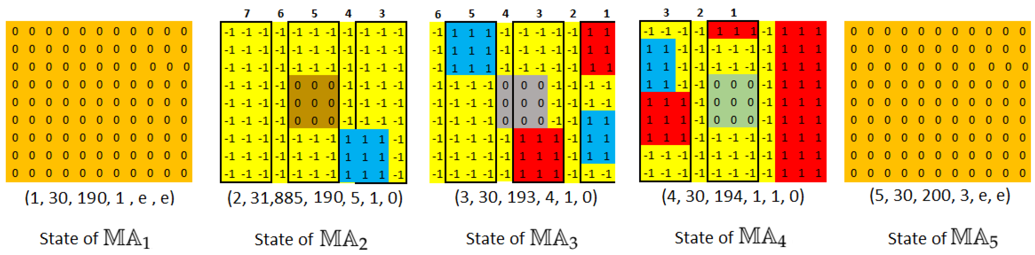
where ${}_2{\mathbf{M}}_{n,m}^{ı}$ is a suitable matrix which enables us to obtain a state matrix with entries given in Figure 7 for the state of ${\mathbb{MA}}_2$. After we apply the input obtained by the internal link ${\phi }_{32}$ in Equation (21) with the help of transition function ${\delta }_2$, we get a new state depicted in Figure 7 for e-quasi-multiautomaton ${\mathbb{MA}}_2$.

Next state of the (vehicle) ${\mathbb{MA}}_4$ will not affect velocity by internal link ${\phi }_{24}$, because the input obtained by ${\phi }_{24}$ from state $\left[\left({}_3{3}^s,{}_3{30}^s,{}_3{192.06}^s,{}_3{3}^s,{}_3{1}^s,{}_3{\frac{\pi }{5}}^s\right){,}_3{\mathbf{T}}_{n,m}^s\right]$ has parameters $\lambda =0$ and $\alpha =0$.

Thus, the input $\left[\left({}_4{4}^{ı},{}_3{\left(\frac{30}{30+1}\right)}^{ı},{}_3{0.99}^{ı},{}_3{0}^{ı},{}_3{1}^{ı},{}_3{0}^s\right),{}_3{\mathbf{N}}_{m,n}^{ı}\right]$ operates as neutral input on states of ${\mathbb{MA}}_4$ except for the distance given by ${}_4{s}_3^s$. Thus, we will present a new situation on the lanes, i.e., a new state after the application of one input. See Figure 7.

4. Conclusions

In this paper, we presented the concept of cartesian compositions, which was first introduced by W. Dörfler. In the past, cartesian compositions were generalized in the sense of hyperstructure theory (using complete hypergroups). Now we considered the internal link between the cartesian product of state sets. We described these internal links by matrices and decision functions. These functions determine which state will influence other components. Our modified concept of the cartesian composition is suitable to describe and control systems used for real-life applications, as was shown in examples throughout the paper. While constructing our system called $\mathcal{S}\mathbb{MA}il$, we assumed that it was made up of e-quasi-multiautomata of a similar nature. This fact affected the proof of the E-GMAC condition (see Theorem 4), which was a substantial simplification of the procedure discussed in [13]. In our future research, we shall concentrate on answering the question of whether the internal link may not remove the necessity to use the extensions of GMAC, i.e., whether the pure GMAC could be used instead of E-GMAC.

References

- Corsini, P.; Leoreanu, V. Applications of Hyperstructure Theory; Kluwer Academic Publishers: Dodrecht, The Netherlands; Boston, MA, USA; London, UK, 2003. [Google Scholar]
- Davvaz, B.; Leoreanu–Fotea, V. Applications of Hyperring Theory; International Academic Press: Palm Harbor, FL, USA, 2007. [Google Scholar]
- Chvalina, J.; Smetana, B. Series of Semihypergroups of Time-Varying Artificial Neurons and Related Hyperstructures. Symmetry 2019, 11, 927. [Google Scholar] [CrossRef] [Green Version]
- Cristea, I.; Kocijan, J.; Novák, M. Introduction to Dependence Relations and Their Links to Algebraic Hyperstructures. Mathematics 2019, 7, 885. [Google Scholar] [CrossRef] [Green Version]
- Křehlík, Š.; Vyroubalová, J. The Symmetry of Lower and Upper Approximations, Determined by a Cyclic Hypergroup, Applicable in Control Theory. Symmetry 2020, 12, 54. [Google Scholar] [CrossRef] [Green Version]
- Novák, M.; Křehlík, Š. EL–hyperstructures revisited. Soft. Comput. 2018, 22, 7269–7280. [Google Scholar] [CrossRef]
- Al Tahan, M.; Hoskova-Mayerova, Š.; Davvaz, B. Some Results on (Generalized) Fuzzy Multi-Hv-Ideals of Hv-Rings. Symmetry 2019, 11, 1376. [Google Scholar] [CrossRef] [Green Version]
- Chvalina, J. Functional Graphs, Quasi-Ordered Sets and Commutative Hypergroups; Masaryk University: Brno, Czech Republic, 1995. (In Czech) [Google Scholar]
- Dörfler, W. The cartesian composition of automata. Math. Syst. Theory 1978, 11, 239–257. [Google Scholar] [CrossRef]
- Gécseg, F.; Peák, I. Algebraic Theory of Automata; Akadémia Kiadó: Budapest, Hungary, 1972. [Google Scholar]
- Ginzburg, A. Algebraic Theory of Automata; Academic Press: New York, NY, USA, 1968. [Google Scholar]
- Novák, M.; Křehlík, Š.; Staněk, D. n-ary Cartesian composition of automata. Soft. Comput. 2019, 24, 1837–1849. [Google Scholar] [CrossRef]
- Chvalina, J.; Křehlík, Š.; Novák, M. Cartesian composition and the problem of generalising the MAC condition to quasi-multiautomata. An. Univ. Ovidius Constanta-Ser. Mat. 2016, 24, 79–100. [Google Scholar]
- Ashrafi, A.R.; Madanshekaf, A. Generalized action of a hypergroup on a set. Ital. J. Pure Appl. Math. 1998, 15, 127–135. [Google Scholar]
- Chvalina, J. Infinite multiautomata with phase hypergroups of various operators. In Proceedings of the 10th International Congress on Algebraic Hyperstructures and Applications, Brno, Czech Republic, 3 September 2008; Hošková, Š., Ed.; University of Defense: Washington, DC, USA; pp. 57–69.
- Chvalina, J.; Chvalinová, L. State hypergroups of automata. Acta Math. Inform. Univ. Ostrav. 1996, 4, 105–120. [Google Scholar]
- Chvalina, J.; Hošková-Mayerová, Š.; Dehghan Nezhad, A. General actions of hyperstructures and some applications. An. Univ. Ovidius Constanta-Ser. Mat. 2013, 21, 59–82. [Google Scholar] [CrossRef]
- Massouros, G.G. Hypercompositional structures in the theory of languages and automata. An. Şt. Univ. A.I. Çuza Iaşi, Sect. Inform. 1994, 3, 65–73. [Google Scholar]
- Dörfler, W. The direct product of automata and quasi-automata. In Mathematical Foundations of Computer Science: 5th Symposium; Mazurkiewicz, A., Ed.; Springer: Gdansk, Poland, 1976; pp. 6–10. [Google Scholar]
- Chvalina, J.; Novák, M.; Křehlík, Š. Hyperstructure generalizations of quasi-automata induced by modelling functions and signal processing. In Proceedings of the 16th International Conference of Numerical Analysis and Applied Mathematics, Rhodes, Greece, 13–18 September 2018. [Google Scholar]
- Křehlík, Š.; Novák, M. Modifed Product of Automata as a Better Tool for Description of Real-Life Systems. In Proceedings of the 17th International Conference of Numerical Analysis and Applied Mathematics, Rhodes, Greece, 23–29 September 2019. [Google Scholar]
- Golestan, K.; Seifzadeh, S.; Kamel, M.; Karray, F.; Sattar, F. Vehicle Localization in VANETs Using Data Fusion and V2V Communication. In Proceedings of the Second ACM International Symposium on Designand Analysis of Intelligent Vehicular Networks and Applications, Paphos, Cyprus, 21 October 2012; pp. 123–130. [Google Scholar]
- Novák, N.; Křehlík, Š.; Ovaliadis, K. Elements of hyperstructure theory in UWSN design and data aggregation. Symmetry 2019, 11, 734. [Google Scholar] [CrossRef] [Green Version]
- Dresner, K.; Stone, P. A multiagent approach to autonomous intersection management. J. Artif. Intell. Res. 2008, 31, 591–656. [Google Scholar] [CrossRef] [Green Version]
- Fajardo, D.; Au, T.-C.; Waller, S.T.; Stone, P.; Yang, D. Automated Intersection Control: Performance of Future Innovation Versus Current Traffic Signal Control. Transp. Res. Rec. 2011, 2259, 223–232. [Google Scholar] [CrossRef] [Green Version]
- Huifu, J.; Jia, H.; Shi, A.; Meng, W.; Byungkyu, B.P. Eco approaching at an isolated signalized intersection under partially connected and automated vehicles environment. Transp. Res. Part C Emerg. Technol. 2017, 79, 290–307. [Google Scholar]
- Latombe, J. Robot Motion Planning; Kluwer Academic Publishers: Boston, MA, USA, 1991. [Google Scholar]
- Liu, F.; Naraynan, A.; Bai, Q. Effective methods for generating collision free paths for multiple robots based on collision type (demonstration). In Proceedings of the 11th International Conference on Autonomous Agents and Multiagent Systems, Valencia, Spain, 4–8 June 2012; Volume 3, pp. 1459–1460. [Google Scholar]
Figure 1.
—A system of multiautomata with internal links.
Figure 2.
Lane shifting.
Figure 3.
Lane shifting; grid view of vehicle .
Figure 4.
Lane change.
Figure 5.
for lane change.
Figure 6.
Complete situation in lanes with detection field of each vehicle.
Figure 7.
A new state of with the release position.
© 2020 by the author. Licensee MDPI, Basel, Switzerland. This article is an open access article distributed under the terms and conditions of the Creative Commons Attribution (CC BY) license (http://creativecommons.org/licenses/by/4.0/).
Share and Cite
MDPI and ACS Style
Křehlík, Š. n-Ary Cartesian Composition of Multiautomata with Internal Link for Autonomous Control of Lane Shifting. Mathematics 2020, 8, 835. https://doi.org/10.3390/math8050835
AMA Style
Křehlík Š. n-Ary Cartesian Composition of Multiautomata with Internal Link for Autonomous Control of Lane Shifting. Mathematics. 2020; 8(5):835. https://doi.org/10.3390/math8050835
Chicago/Turabian StyleKřehlík, Štěpán. 2020. "n-Ary Cartesian Composition of Multiautomata with Internal Link for Autonomous Control of Lane Shifting" Mathematics 8, no. 5: 835. https://doi.org/10.3390/math8050835
Note that from the first issue of 2016, this journal uses article numbers instead of page numbers. See further details here.