Predicting Hard Rock Pillar Stability Using GBDT, XGBoost, and LightGBM Algorithms


1
School of Resources and Safety Engineering, Central South University, Changsha 410083, China
2
The Robert M. Buchan Department of Mining, Queen’s University, Kingston, ON K7L 3N6, Canada
3
College of Systems Engineering, National University of Defense Technology, Changsha 410073, China
*
Author to whom correspondence should be addressed.
Mathematics 2020, 8(5), 765; https://doi.org/10.3390/math8050765
Submission received: 17 April 2020
/
Revised: 5 May 2020
/
Accepted: 8 May 2020
/
Published: 11 May 2020
Abstract
:Predicting pillar stability is a vital task in hard rock mines as pillar instability can cause large-scale collapse hazards. However, it is challenging because the pillar stability is affected by many factors. With the accumulation of pillar stability cases, machine learning (ML) has shown great potential to predict pillar stability. This study aims to predict hard rock pillar stability using gradient boosting decision tree (GBDT), extreme gradient boosting (XGBoost), and light gradient boosting machine (LightGBM) algorithms. First, 236 cases with five indicators were collected from seven hard rock mines. Afterwards, the hyperparameters of each model were tuned using a five-fold cross validation (CV) approach. Based on the optimal hyperparameters configuration, prediction models were constructed using training set (70% of the data). Finally, the test set (30% of the data) was adopted to evaluate the performance of each model. The precision, recall, and F1 indexes were utilized to analyze prediction results of each level, and the accuracy and their macro average values were used to assess the overall prediction performance. Based on the sensitivity analysis of indicators, the relative importance of each indicator was obtained. In addition, the safety factor approach and other ML algorithms were adopted as comparisons. The results showed that GBDT, XGBoost, and LightGBM algorithms achieved a better comprehensive performance, and their prediction accuracies were 0.8310, 0.8310, and 0.8169, respectively. The average pillar stress and ratio of pillar width to pillar height had the most important influences on prediction results. The proposed methodology can provide a reliable reference for pillar design and stability risk management.
1. Introduction
Pillars are essential structural units to ensure mining safety in underground hard rock mines. Their functions are to provide safe access to working areas, and support the weight of overburden rocks for guaranteeing global stability [1,2]. Instable pillars can cause large-scale catastrophic collapse, and significantly increase safety hazards of workers [3]. If a pillar fails, the adjacent pillars have to bear a larger load. The increased load may exceed the strength of adjacent pillars, and lead to their failure. Like the domino effect, rapid and large-scale collapse can be induced [4]. In addition, with the increase of mining depth, the ground stress is larger and pillar instability accidents become more frequent [5,6,7]. Accordingly, determining pillar stability is essential for achieving safe and efficient mining.
In general, there are three types of methods to determine pillar stability in hard rock mines. The first one is the safety factor approach. The safety factor indicates the ratio of pillar strength to stress [8]. Using this method, three parts, namely, pillar strength, pillar stress, and safety threshold, should be determined. For the calculation of pillar strength, many empirical methods have been proposed, such as the linear shape effect, power shape effect, size effect, and Hoek–Brown formulas [9]. For the determination of pillar stress, tributary area theory, and numerical modeling technology are the main approaches [10]. Based on the pillar strength and stress, the safety factor can be calculated. A larger safety factor means the pillar is more stable. Theoretically, the safety threshold is assigned as 1. If the safety factor is larger than 1, the pillar is stable, otherwise it is unstable [11]. Considering the possible deviations of this method, the safety threshold is generally larger than 1 to ensure safety in practice. Although the safety factor method is simple, the unified pillar strength formula and safety threshold are still not determined.
The second one is the numerical simulation technique. Numerical simulation methods have been widely used because the complicated boundary conditions and rock mass properties can be considered. Mortazavi et al. [12] adopted fast Lagrangian analysis of continua (FLAC) approach to study the failure process and non-linear behavior of rock pillars; Shnorhokian et al. [13] used FLAC3D to assess the pillar stability based on different mining sequence scenarios; Elmo and Stead [14] integrated finite element method (FEM) and discrete element method (DEM) to investigate the failure characteristics of naturally fractured pillars; Li et al. [15] used rock failure process analysis (RFPA) to evaluate the pillar stability under coupled thermo-hydrologic-mechanical conditions; Jaiswal et al. [16] utilized boundary element method (BEM) to simulate asymmetry in the induced stresses over pillars; and Li et al. [17] introduced finite-discrete element method (FDEM) to analyze the mechanical behavior and failure mechanisms of the pillar. In addition, some scholars combined numerical simulation and other mathematical models to study pillar stability. Deng et al. [18] used FEM, neural networks, and reliability analysis to optimize pillar design; and Griffiths et al. [19] adopted random field theory, elastoplastic finite element algorithm and Monte-Carlo approach to analyze pillar failure probability. Using numerical simulation techniques, the complex failure behaviors of pillars can be modeled and the failure process and range can be obtained. However, because of the complicated nonlinear characteristics and anisotropic nature of rock mass, the model inputs and constitutive equations are not easy to be accurately determined [20]. Therefore, the reliability of results obtained by this method is limited.
The third one is the machine learning (ML) algorithm. Big data has been proved to be useful for managing emergencies and disasters [21]. With the accumulation of pillar stability cases, it provides researchers the opportunity to develop advanced predictive models using ML algorithms. Tawadrous and Katsabanis [22] used the artificial neural networks (ANN) to analyze the stability of surface crown pillars; Wattimena [23] introduced the multinomial logistic regression (MLR) for pillar stability prediction; Ding et al. [24] adopted a stochastic gradient boosting (SGB) model to predict pillar stability, and found that this model achieved a better performance than the random forest (RF), support vector machine (SVM), and multilayer perceptron neural networks (MPNN); Ghasemi et al. [25] utilized J48 algorithm and SVM to develop two pillar stability graphs, and obtained acceptable prediction accuracy; and Zhou et al. [9] compared the prediction performance of pillar stability using six supervised learning methods, and revealed that SVM and RF performed better. Although these ML algorithms can solve pillar stability prediction issues to some extent, none can be applied to all engineering conditions. To date, there is not a uniform algorithm under the consensus of the mining industry.
Compared with traditional safety factor and numerical simulation methods, ML approach can deeply find implicit relationships between variables, and well handle nonlinear problems. Therefore, it is a promising method for predicting pillar stability. In addition to these above ML algorithms, the gradient boosting decision tree (GBDT) method has shown great prediction performances in many fields [26,27,28]. As one of the ensemble learning algorithms, it integrates multiple decision trees (DTs) into a strong classifier using the boosting approach [29]. DTs refer to a ML method using tree-like structure, which can deal with various types of data and trace every path to the prediction results [30]. However, DTs are easy to overfit and sensitive to noises of the dataset. Through the integration of DTs, the overall prediction performances of GBDT become better because the errors of DTs are compensated by each other. Under the framework of GBDT, extreme gradient boosting (XGBoost) [31] and light gradient boosting machine (LightGBM) [32] have been proposed recently. They have also received wide attentions because of their excellent performances. Particularly, these three algorithms work well with small datasets. Additionally, overfitting, which means the model fits the existing data too exactly but fails to predict the future data reliably, can be avoided to some extent [30]. However, to the best of our knowledge, GBDT, XGBoost, and LightGBM algorithms have not been used to predict pillar stability in hard rock mines.
The objective of this study is to predict hard rock pillar stability using GBDT, XGBoost, and LightGBM algorithms. First, pillar stability cases are collected from seven hard rock mines. Next, these three algorithms are applied to predict pillar stability. Finally, their comprehensive performances are analyzed and compared with the safety factor approach and other ML algorithms.
2. Data Acquisition
The existing hard rock pillar cases are obtained as supportive data for the establishment of prediction model. In this study, 236 samples were collected from seven underground hard rock mines [8,10,33]. These mines include the Elliot Lake uranium mine, Selebi-Phikwe mine, Open stope mine, Zinkgruvan mine, Westmin Resources Ltd.’s H-W mine, Marble mine, and Stone mine. The pillar stability data is shown in Table 1 (the complete database is available in Table S1), where indicates the pillar width, indicates the pillar height, indicates the ratio of pillar width to pillar height, indicates the uniaxial compressive strength, and indicates the average pillar stress.
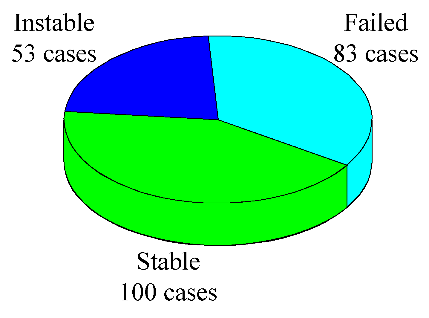
From Table 1, it can be seen that each sample contains five indicators and the level of pillar stability. These five indicators have been widely used in a large amount of literature [9,10,24,33]. The advantages are two-fold: (1) They can reflect the necessary conditions of pillar stability, such as pillar size, strength, and load; (2) their values are relatively easy to be obtained. The descriptive statistics of each indicator are listed in Table 2. Besides, according to the instability mechanism and failure process of pillars, the level of pillar stability is divided into three types: stable, instable, and failed. Among them, the stable level indicates that the pillar shows no sign of stress induced fracturing, or only has minor spallings which do not affect pillar stability; the instable level indicates that the pillar is partially failed, and has prominent spallings, but still possesses a certain supporting capacity; the failed level indicates that the pillar is crushed, and has pronounced openings of joints, which shows a great collapse risk. The distribution of these three pillar stability levels is described in Figure 1.
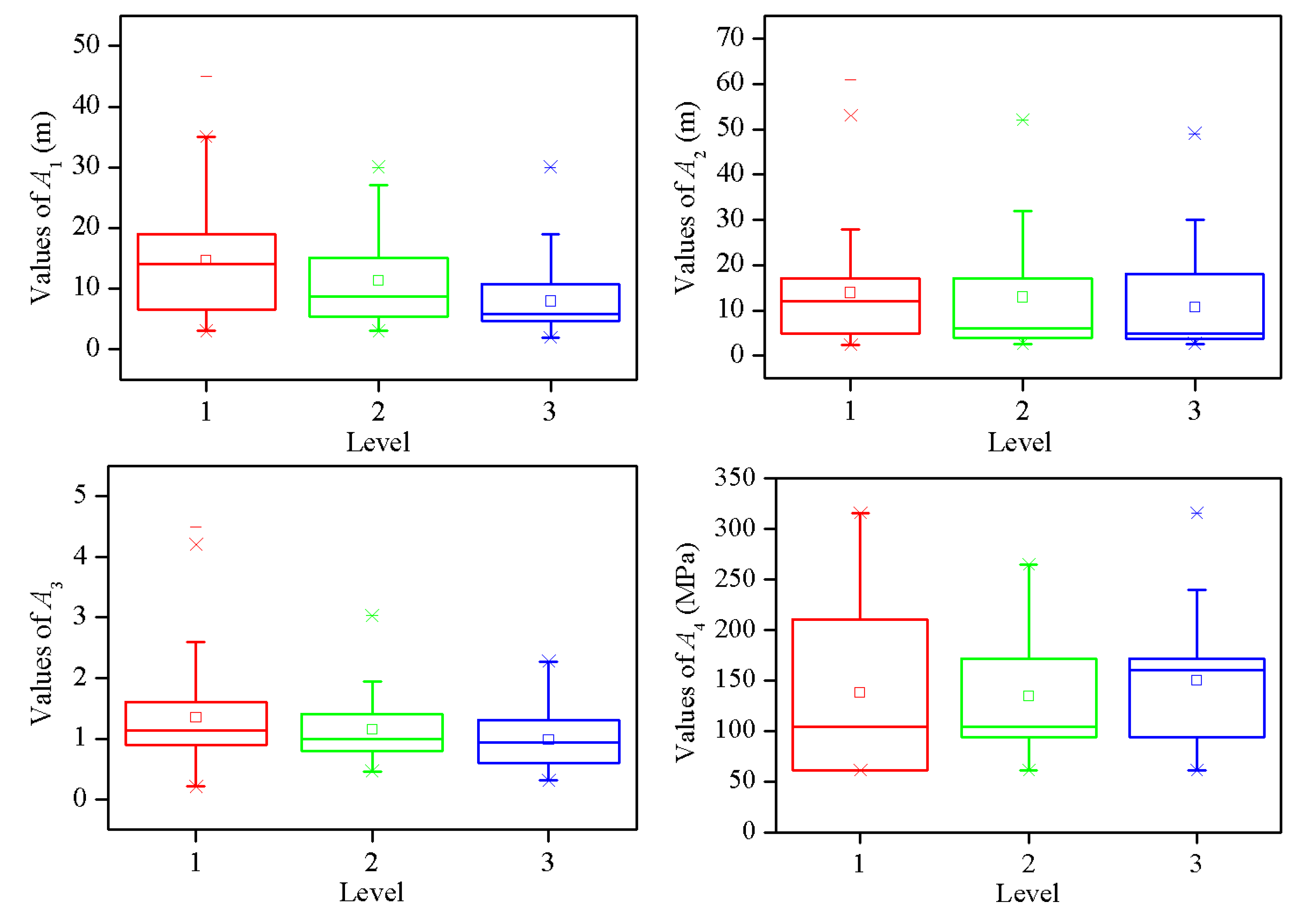
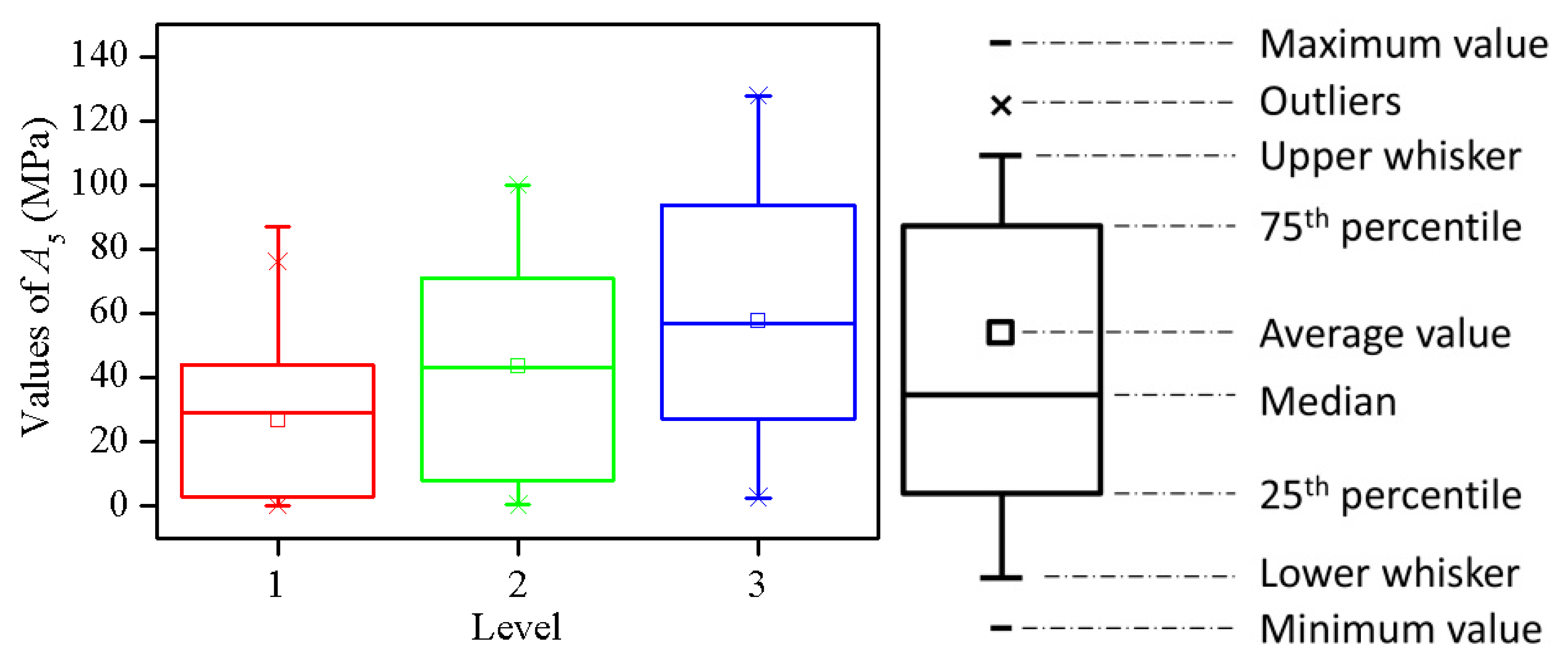
The box plot of each indicator for different pillar stability level is shown in Figure 2. According to Figure 2, some meaningful characteristics can be found. First, all indicators have several outliers. Second, the pillar stability level is negatively correlated with and (the Pearson correlation coefficients are −0.381 and −0.266, respectively), while is positively correlated with (the Pearson correlation coefficient is 0.433). However, there are no obvious correlations with and (the Pearson correlation coefficients are −0.121 and 0.079, respectively). Third, the distances between upper and lower quartiles are different for the same indicators in various levels. Fourth, there are some overlapping parts for the range of indicator values in different levels. Fifth, as the median is not in the center of the box, the distribution of indicator values is asymmetric. All these phenomena illustrate the complexity of pillar stability prediction.
3. Methodology
3.1. GBDT Algorithm
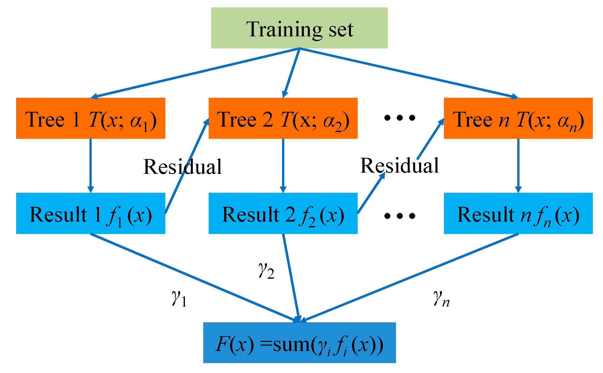
GBDT is an ensemble ML algorithm using multiple DTs as base learners. Every decision tree (DT) is not independent, because a new added DT increases emphasis on the misclassified samples attained by previous DTs [34]. The diagram of GBDT algorithm is shown in Figure 3. It can be noticed that the residual of former DTs is taken as the input for the next DT. Then, the added DT is used to reduce residual, so that the loss decreases following the negative gradient direction in each iteration. Finally, the prediction result is determined based on the sum of results from all DTs.
Let indicates the sample data, where represent the indicators, and denotes the label. The specific steps of GBDT are indicated as follows [35]:
Step 1: The initial constant value is obtained as
where is the loss function.
Step 2: The residual along the gradient direction is written as
where indicates the number of iterations, and .
Step 3: The initial model is obtained by fitting sample data, and the parameter is calculated based on the least square method as
Step 4: By minimizing the loss function, the current model weight is expressed as
Step 5: The model is updated as
This loop is performed until the specified iterations times or the convergence conditions are met.
3.2. XGBoost Algorithm
XGBoost algorithm was proposed by Chen and Guestrin [31] based on the GBDT structure. It has received widespread attentions because of its excellent performances in Kaggle’s ML competitions [36]. Different from the GBDT, XGBoost introduces the regularization term in the objective function to prevent overfitting. The objective function is defined as
where denotes the regularization term at the time iteration, and is a constant term, which can be selectively omitted.
The regularization term is expressed as
where represents the complexity of leaves, indicates the number of leaves, denotes the penalty parameter, and is the output result of each leaf node. In particular, the leaves indicate the predicted categories following the classification rules, and the leaf node indicates the node of the tree that cannot be split.
Moreover, as opposed to use the first-order derivative in GBDT, a second-order Taylor series of objective function is adopted in XGBoost. Suppose the mean square error is used as the loss function, then the objective function can be derived as
where indicates a function that assigns data points to the corresponding leaves, and and denote the first and second derivative of loss function, respectively.
The final loss value is calculated based on the sum of all loss values. Because samples correspond to leaf nodes in the DT, the ultimate loss value can be determined by summing the loss values of leaf nodes. Therefore, the objective function is also expressed as
where , , and indicates all samples in leaf node .
To conclude, the optimization of objective function is converted to a problem of determining the minimum of a quadratic function. In addition, because of the introduction of regularization term, XGBoost has a better ability to against overfitting.
3.3. LightGBM Algorithm
LightGBM was another algorithm designed by Microsoft Research Asia [32] using GBDT framework. It aims to improve the computational efficiency, so that the prediction problems with big data can be solved more effectively. In GBDT algorithm, presorting approach is used to select and split indicators. Although this method can precisely determine the splitting point, it requires more time and memory. In LightGBM, the histogram-based algorithm and trees leaf-wise growth strategy with a maximum depth limit is adopted to increase the training speed and reduce memory consumption.
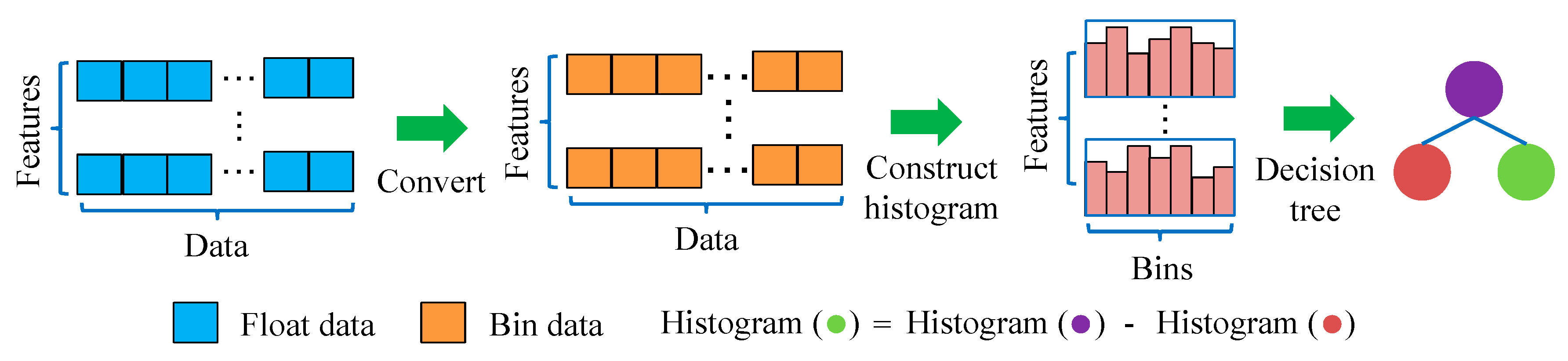
The histogram-based DT algorithm is shown in Figure 4. It can be seen that the successive floating-point eigenvalues are discretized into s small bins. After that, these bins are used to construct the histogram with width s. Once the data is traversed at the first time, the required statistics (sum of gradients and number of samples in each bin) are accumulated in the histogram. Based on the discrete value of histogram, the optimal segmentation point can be found [37]. By using this method, the cost of storage and calculation can be reduced.
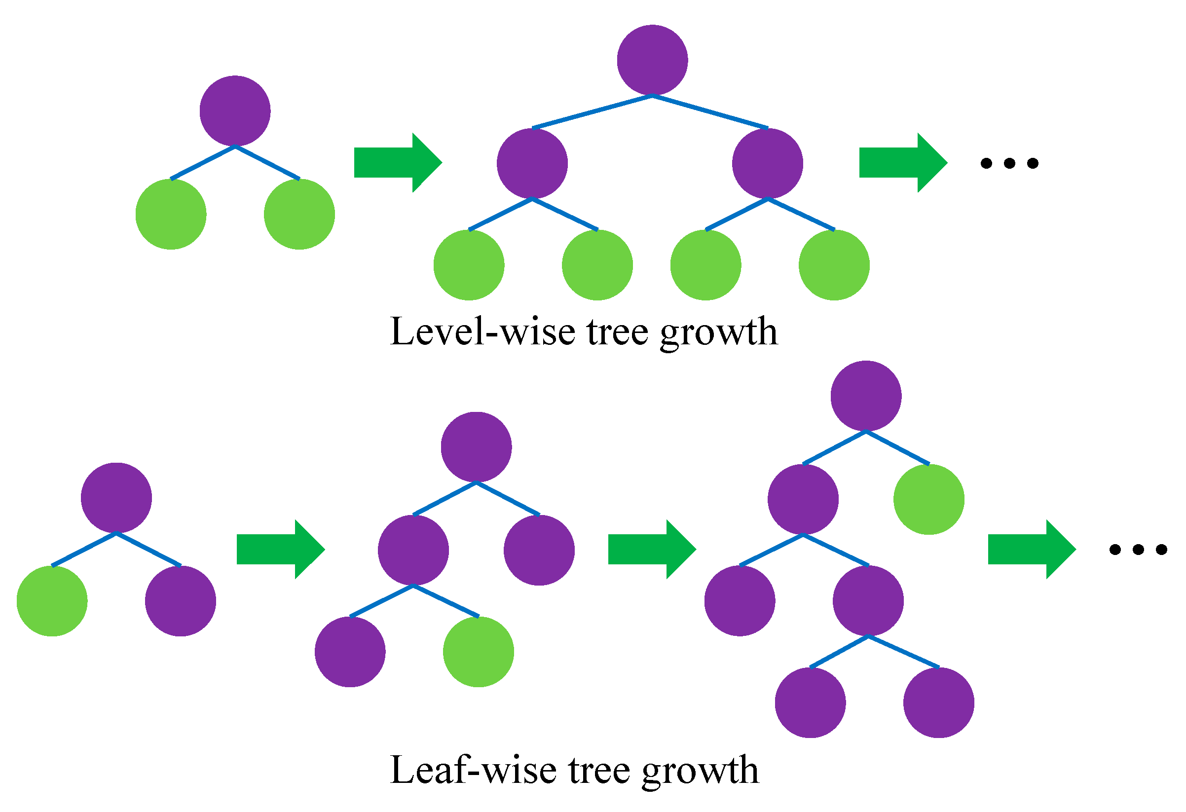
The level-wise and leaf-wise growth strategies are shown in Figure 5. According to the level-wise growth strategy, the leaves on the same layer are simultaneously split. It is favorable to optimize with multiple threads, and control model complexity. However, leaves on same layer are indiscriminately treated, whereas they have different information gain. Information gain indicates the expected reduction in entropy caused by splitting the nodes based on attributes, which can be determined by [38]
where is the information entropy of the collection , is the ratio of pertaining to category , is the number of categories, is the value of attribute , and is the subset of for which attribute has value .
Actually, many leaves with low information gain are unnecessary to be searched and split, which increases a great deal of extra memory consumption and causes this method to be ineffective. In contrast, leaf-wise growth strategy is more efficient because it only split the leaf that has the largest information gain on the same layer. Furthermore, considering this strategy may cause trees with high depth, resulting in overfitting, a maximum depth limitation is adopted during the growth of trees [39].
4. Construction of Prediction Model
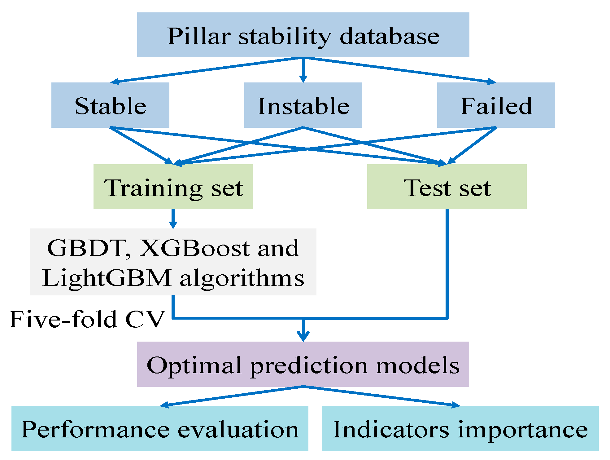
The construction process of prediction model is shown in Figure 6. First, approximately 70% and 30% of the original pillar stability data are selected as training and test sets, respectively. Second, a five-fold cross validation (CV) approach is utilized to tune the model hyperparameters. Third, using the optimal hyperparameters configuration, the prediction model is fitted based on training set. Fourth, the test set is adopted to evaluate model performances according to the overall prediction results and the prediction ability for each stability level. Last, by comparing the comprehensive performance of these models, the optimal model is determined. If the prediction performance of this model is acceptable, then it can be adopted for deployment. The entire calculation process is performed in Python 3.7 based on the scikit-learn [40], XGBoost [41], and LightGBM [42] libraries, respectively. The hyperparameter optimization process and model evaluation indexes are descripted as follows.
4.1. Hyperparameter Optimization
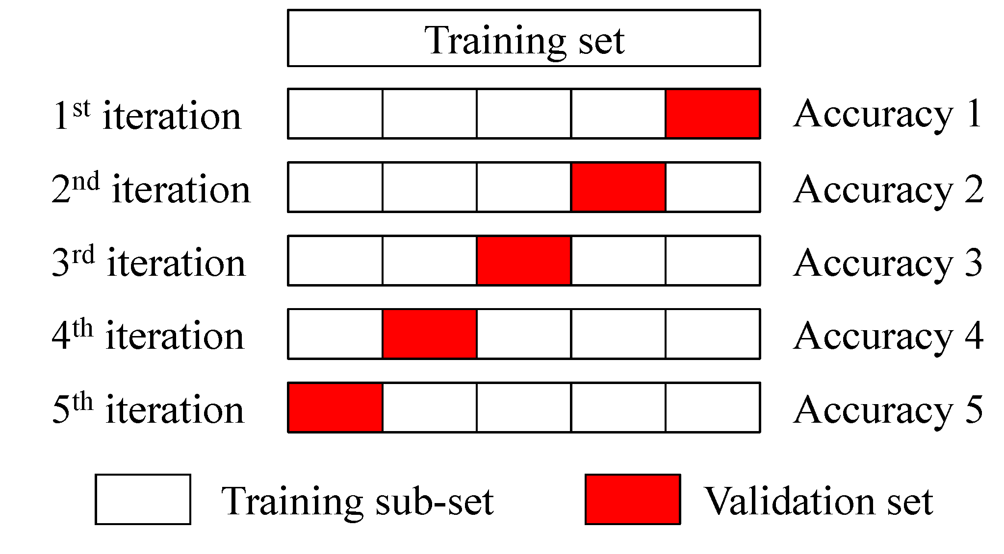
Most of ML algorithms contain hyperparameters that need to be tuned. These hyperparameters should be adjusted based on dataset rather than specifying manually. Generally, the hyperparameters search methods include grid search, Bayesian optimization, heuristic search and randomized search [43]. Because the randomized search method is more efficient for simultaneously tuning multiple hyperparameters, it is used to recognize the best set of hyperparameters in this study. In general, K-fold CV approach is utilized for hyperparameters configuration [44]. In our work, five-fold CV method is used, which is illustrated in Figure 7. The original training set is randomly split into five equal size subsamples. Among them, a singular subsample is adopted as the validation set, and the other four subsamples are used as the training sub-set. This procedure is repeated five times until each subsample is selected as a validation set once. Thereafter, the average accuracy of these five validation sets is used to determine the optimal hyperparameter values.
In this study, some critical hyperparameters in GBDT, XGBoost, and LightGBM algorithms are tuned, as shown in Table 3. The specific meanings of these hyperparameters are also explained in Table 3. First, the search range of different hyperparameters values is specified. In particular, for different algorithms, the search range of the same hyperparameters is kept consistent. Further on, according to the maximum average accuracy, the optimal values for each set of hyperparameters are obtained, which are indicted in Table 3.
4.2. Model Evaluation Indexes
The accuracy, precision, recall and measures have been widely used for the performance evaluation of ML algorithms [43]. Among them, accuracy indicates the proportion of samples that is correctly predicted; precision is the ability to accurately predict samples; recall denotes the capability of correctly predicting as many samples as possible in actual samples; and represents a comprehensive metric that measures the performance of both precision and recall. Accordingly, these indexes are adopted to evaluate model performances in this study. Assume the confusion matrix is expressed as
where is the number of pillar stability levels, represents the number of samples correctly predicted for level , and denotes the number of samples of level that are classified to level .
Based on the confusion matrix, the precision, recall and measure for each pillar stability level are respectively determined by
To further reflect the overall prediction performance, the accuracy and macro average of precision, recall and F1 (expressed as , and , respectively) are calculated as
5. Results and Analysis
5.1. Overall Prediction Results
The prediction results of GBDT, XGBoost, and LightGBM algorithms were obtained on the test set. Subsequently, the confusion matrix of each algorithm was determined, as shown in Table 4. The values on the main diagonal indicated the number of samples correctly predicted. It can be seen that most samples were accurately classified using these three algorithms. Based on Table 4, the accuracy, , , and were calculated based on Equations (16)–(19), which were listed in Table 5. According to the results, all these three algorithms had good performances in predicting the pillar stability of hard rock. Furthermore, the accuracy degrees of GBDT and XGBoost were largest and up to 0.8310, followed by LightGBM with an accuracy of 0.8169. Although GBDT and XGBoost possessed the same accuracy, the prediction performances were different. Comparing their values of , , and , GBDT performed better than XGBoost. Therefore, based on their overall prediction performances, the rank was GBDT > XGBoost > LightGBM.
5.2. Prediction Results of Each Stability
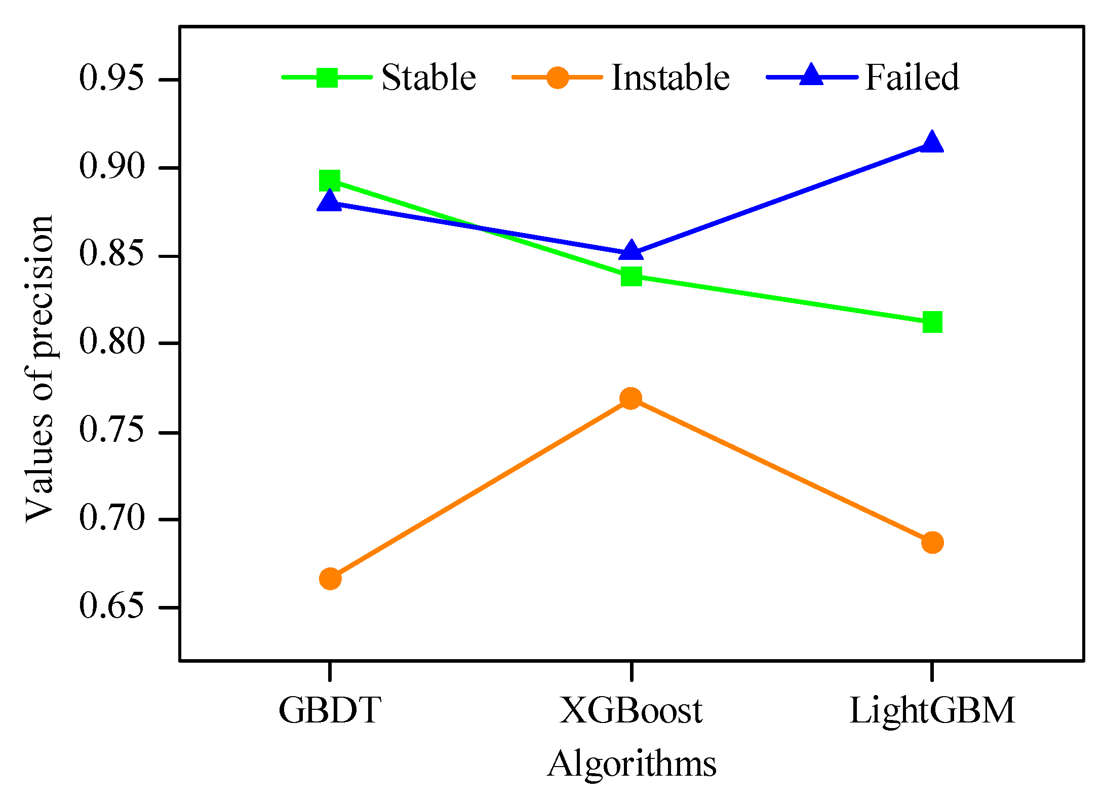
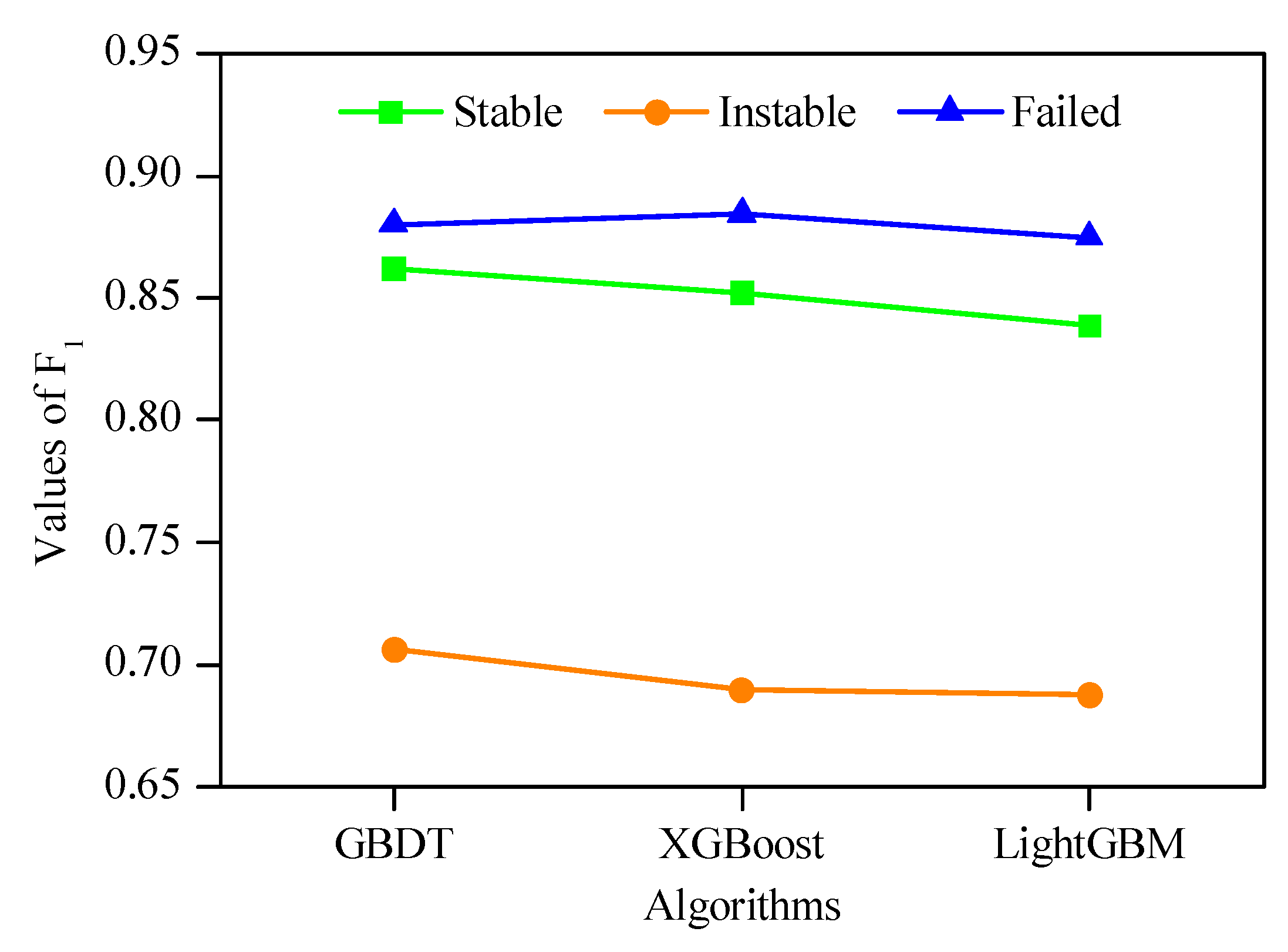
To analyze the prediction performance of algorithms for each stability level, the precision, recall and F1 indexes were calculated based on Equations (13)–(15), which were shown in Figure 8, Figure 9 and Figure 10, respectively. It can be seen that the prediction performance of each algorithm for different stability level was not the same. For the stable level, GBDT achieved the highest precision value (0.8929) and the highest F1 value (0.8621); and XGBoost achieved the highest recall value (0.8667). For the instable level, XGBoost possessed the highest precision value (0.7692); and GBDT possessed the highest recall value (0.7500) and the highest F1 value (0.7059). For the failed level, LightGBM obtained the highest precision value (0.9130); and XGBoost obtained the highest recall value (0.9200) and the highest F1 value (0.8846). Moreover, it can be observed that the prediction performance of these algorithms for failed level was the best, followed by stable level. However, the prediction performance for instable level was the worst.
5.3. Relative Importance of Indicators
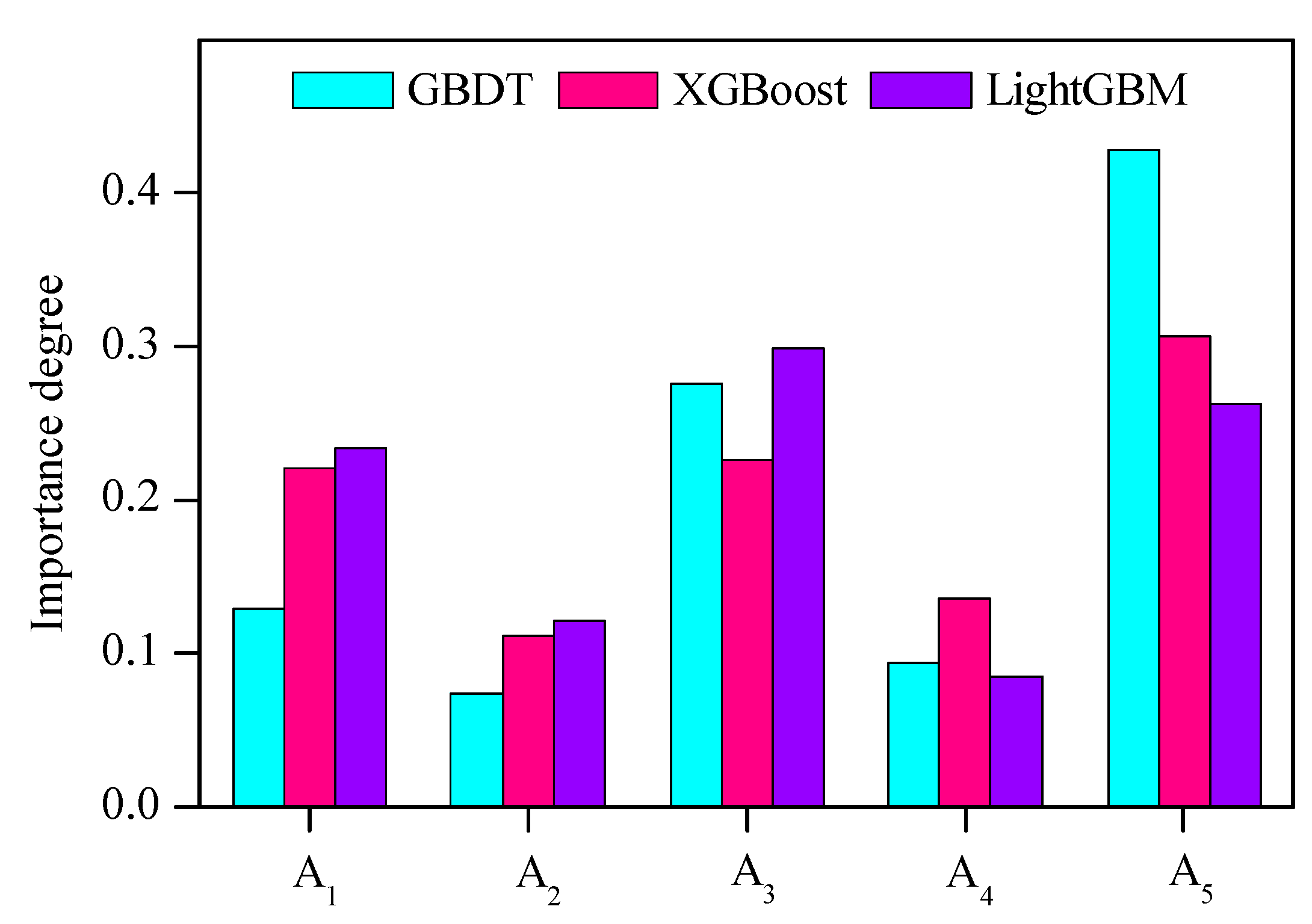
The relative importance of indicators is a valuable reference for taking reasonable measures to prevent pillar instability. In this study, the importance degree of each indicator was obtained using GBDT, XGBoost, and LightGBM algorithms, which was indicated in Figure 11. Based on GBDT algorithm, the rank of importance degree was . According to XGBoost algorithm, the rank of importance degree was . Using LightGBM algorithm, the rank of importance degree was . Therefore, there were two most important indicators: (average pillar stress) and (ratio of pillar width to pillar height).
6. Discussions
Although the pillar stability can be well predicted using GBDT, XGBoost, and LightGBM algorithms, the prediction performance for different instable level was not the same. The reason may be two-fold. One is that the number of samples for instable level is smaller than other two levels. Another is that the discrimination boundary of instable level is more uncertain, which would influence the quality of data. As data-driven approaches, the prediction performances of GBDT, XGBoost, and LightGBM algorithms are greatly affected by the number and quality of supportive data. Therefore, compared with other two levels, the prediction performance for instable level was worse.
According to the analysis of indicator importance, and were the most important indicator. The reason may be that the pillar stability is greatly affected by the external stress conditions and inherent dimension characteristics. According to the field experience, the spalling phenomenon of pillar was more common in deep mines because of high stress, and the pillar with small value was more vulnerable to be damaged. Based on the importance degrees of indicators, some measures can be adopted to improve pillar stability from two directions. One is reducing pillar stress, such as the adjustment of excavation sequence and relief of pressure [32]. Another is optimizing pillar parameters, such as the increase of pillar width and ratio of pillar width to pillar height.
To further illustrate the effectiveness of GBDT, XGBoost, and LightGBM algorithms, the safety factor approach and other ML algorithms were adopted as comparisons.
First, the safety factor approach was used to determine pillar stability. According to the research of Esterhuizen et al. [33], the pillar strength can be calculated by
Based on Equation (20) and the given pillar stress, the safety factor can be determined by their quotient. From the work of Lunder and Pakalnis [45], when , the pillar was stable; when , the pillar was unstable; and when , the pillar was failed. According to this discrimination method, the prediction accuracy was 0.6610. From the work of González-Nicieza et al. [8], when , the pillar was stable; when , the pillar was unstable; and when , the pillar was failed. Base on this classification method, the prediction accuracy was 0.6398. Therefore, the prediction accuracy of safety factor approach was lower than that of the proposed methodology. It can be inferred that this empirical method has difficulty in obtaining satisfactory prediction results on these pillar samples.
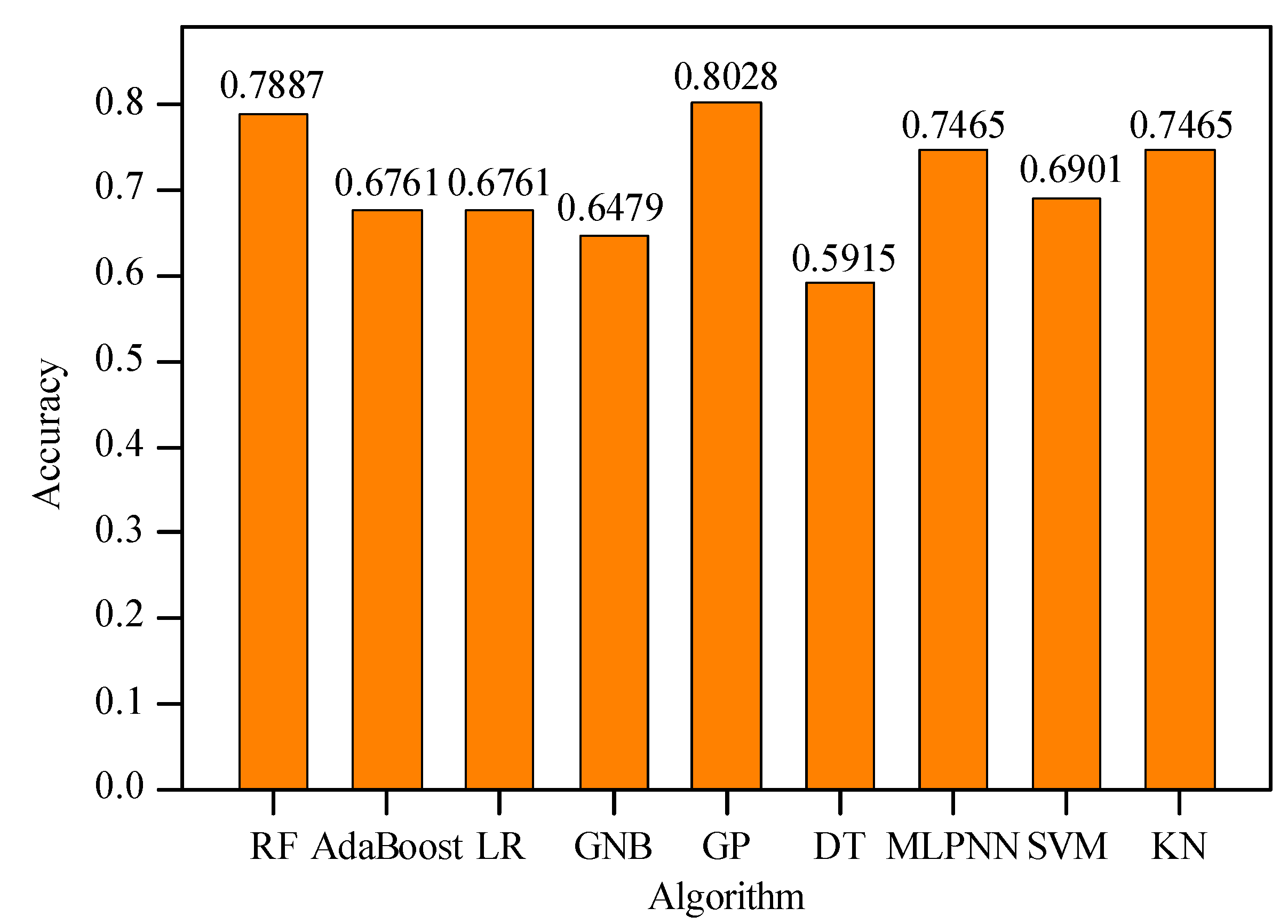
On the other hand, some ML algorithms, such as RF, adaptive boosting (AdaBoost), MLR, Gaussian naive Bayes (GNB), Gaussian processes (GP), DT, MLPNN, SVM, and k-nearest neighbor (KNN), were adopted to predict pillar stability. First, some key hyperparameters in these algorithms were tuned, and the optimization results were listed in Table 6. Afterwards, these algorithms with optimal hyperparameters were used to predict pillar stability based on the same dataset. The accuracy of each algorithm was shown in Figure 12. It can be seen that the accuracies of these algorithms were all lower than those of GBDT, XGBoost, and LightGBM algorithms. The accuracies of most algorithms (except for GP) were lower than 0.8, whereas the accuracies of GBDT, XGBoost, and LightGBM algorithms were all higher than 0.8. It demonstrated that compared with other ML algorithms, GBDT, XGBoost, and LightGBM algorithms were better for predicting pillar stability in hard rock mines.
Although the proposed approach obtains desirable prediction results, some limitations should be addressed in the future.
- (1)
- The dataset is relatively small and unbalanced. The prediction performance of ML algorithms is heavily affected by the number and quality of dataset. Generally, if the dataset is small, the generalization and reliability of model would be influenced. Although GBDT, XGBoost, and LightGBM algorithms work well with small datasets, the prediction performances could be better on a larger dataset. In addition, the dataset is unbalanced, particularly for samples with instable level. Compared with other levels, the prediction performance for the instable level is not good. This illustrates the adverse effects of imbalanced data on results. Therefore, it is meaningful to establish a larger and more balanced pillar stability database.
- (2)
- Other indicators may also have influences on the prediction results. Pillar stability is affected by numerous factors, including the inherent characteristics and external environments. Although the five indictors adopted in this study can describe the necessary conditions of pillar stability to some extent, some other indicators may also have effects on pillar stability, such as joints, underground water, and blasting disturbance. Theoretically, the joints and underground water can affect the pillar strength, and blasting disturbance can be deemed as a dynamic stress on the pillar. Accordingly, it is significant to analyze the influences of these indicators on the prediction results.
7. Conclusions
To ensure mining safety, pillar stability prediction is a crucial task in underground hard rock mines. This study investigated the performance of GBDT, XGBoost, and LightGBM algorithms for pillar stability prediction. The prediction models were constructed based on training set (165 cases) after their hyperparameters were tuned using the five-fold CV method. The test set (71 cases) were adopted to validate the feasibility of trained models. Overall, the performances of GBDT, XGBoost, and LightGBM were acceptable, and their prediction accuracies were 0.8310, 0.8310, and 0.8169, respectively. By comprehensively analyzing the accuracy and macro average of precision, recall and F1, the rank of overall prediction performance was GBDT > XGBoost > LightGBM. According to the precision, recall and F1 of each stability level, the prediction performance for stable and failed levels was better than that for instable level. Based on the importance scores of indicators from these three algorithms, the average pillar stress and ratio of pillar width to pillar height were the most influential indicators on the prediction results. Compared with the safety factor approach and other ML algorithms (RF, AdaBoost, LR, GNB, GP, DT, MLPNN, SVM, and KNN), the performances of GBDT, XGBoost, and LightGBM were better, which further verified that they were reliable and effective for the pillar stability prediction.
In the future, a larger and more balanced pillar stability database can be established to further illustrate the adequacy of these algorithms for the prediction of stable, instable, and failed pillar levels. The influences of other indicators on the prediction results are essential to be analyzed. The methodology can also be applied in other fields, such as the risk prediction of landslide, debris flow, and rockburst.
Supplementary Materials
The following are available online at https://www.mdpi.com/2227-7390/8/5/765/s1, Table S1: Pillar stability cases database.
Author Contributions
This research was jointly performed by W.L., S.L., G.Z., and H.W. Conceptualization, W.L. and S.L.; Methodology, S.L.; Software, G.Z. and H.W.; Validation, G.Z. and H.W.; Formal analysis, H.W.; Investigation, W.L.; Resources, S.L.; Data curation, G.Z. and H.W.; Writing—original draft preparation, W.L.; Writing—review and editing, W.L., S.L., G.Z., and H.W.; Funding acquisition, G.Z. All authors have read and agreed to the published version of the manuscript.
Funding
This research was funded by the National Natural Science Foundation of China (no. 51774321) and National Key Research and Development Program of China (no. 2018YFC0604606).
Conflicts of Interest
The authors declare no conflict of interest.
References
- Ghasemi, E.; Ataei, M.; Shahriar, K. Prediction of global stability in room and pillar coal mines. Nat. Hazards 2014, 72, 405–422. [Google Scholar] [CrossRef]
- Liang, W.Z.; Dai, B.; Zhao, G.Y.; Wu, H. Assessing the Performance of Green Mines via a Hesitant Fuzzy ORESTE–QUALIFLEX Method. Mathematics 2019, 7, 788. [Google Scholar] [CrossRef] [Green Version]
- Wang, J.A.; Shang, X.C.; Ma, H.T. Investigation of catastrophic ground collapse in Xingtai gypsum mines in China. Int. J. Rock Mech. Min. 2008, 45, 1480–1499. [Google Scholar] [CrossRef]
- Zhou, Y.J.; Li, M.; Xu, X.D.; Li, X.T.; Ma, Y.D.; Ma, Z. Research on catastrophic pillar instability in room and pillar gypsum mining. Sustainability 2018, 10, 3773. [Google Scholar] [CrossRef] [Green Version]
- Liang, W.Z.; Zhao, G.Y.; Wu, H.; Chen, Y. Assessing the risk degree of goafs by employing hybrid TODIM method under uncertainty. B. Eng. Geol. Environ. 2019, 78, 3767–3782. [Google Scholar] [CrossRef]
- Peng, K.; Liu,, Z.P.; Zou, Q.L.; Zhang, Z.Y.; Zhou, J.Q. Static and dynamic mechanical properties of granite from various burial depths. Rock Mech. Rock Eng. 2019, 52, 3545–3566. [Google Scholar]
- Luo, S.Z.; Liang, W.Z.; Xing, L.N. Selection of mine development scheme based on similarity measure under fuzzy environment. Neural Comput. Appl. 2019, 32, 5255–5266. [Google Scholar] [CrossRef]
- González-Nicieza, C.; Álvarez-Fernández, M.I.; Menéndez-Díaz, A.; Alvarez-Vigil, A.E. A comparative analysis of pillar design methods and its application to marble mines. Rock Mech. Rock Eng. 2006, 39, 421–444. [Google Scholar] [CrossRef]
- Zhou, J.; Li, X.; Mitri, H.S. Comparative performance of six supervised learning methods for the development of models of hard rock pillar stability prediction. Nat. Hazards 2015, 79, 291–316. [Google Scholar] [CrossRef]
- Lunder, P.J. Hard Rock Pillar Strength Estimation: An Applied Empirical Approach. Master’s Thesis, University of British Columbia, Vancouver, BC, Canada, 1994. [Google Scholar]
- Cauvin, M.; Verdel, T.; Salmon, R. Modeling uncertainties in mining pillar stability analysis. Risk Anal. 2009, 29, 1371–1380. [Google Scholar] [CrossRef]
- Mortazavi, A.; Hassani, F.P.; Shabani, M. A numerical investigation of rock pillar failure mechanism in underground openings. Comput. Geotech. 2009, 36, 691–697. [Google Scholar] [CrossRef]
- Shnorhokian, S.; Mitri, H.S.; Moreau-Verlaan, L. Stability assessment of stope sequence scenarios in a diminishing ore pillar. Int. J. Rock Mech. Min. 2015, 74, 103–118. [Google Scholar] [CrossRef]
- Elmo, D.; Stead, D. An integrated numerical modelling–discrete fracture network approach applied to the characterisation of rock mass strength of naturally fractured pillars. Rock Mech. Rock Eng. 2010, 43, 3–19. [Google Scholar] [CrossRef]
- Li, L.C.; Tang, C.A.; Wang, S.Y.; Yu, J. A coupled thermo-hydrologic-mechanical damage model and associated application in a stability analysis on a rock pillar. Tunn. Undergr. Space Technol. 2013, 34, 38–53. [Google Scholar] [CrossRef]
- Jaiswal, A.; Sharma, S.K.; Shrivastva, B.K. Numerical modeling study of asymmetry in the induced stresses over coal mine pillars with advancement of the goaf line. Int. J. Rock Mech. Min. 2004, 41, 859–864. [Google Scholar] [CrossRef]
- Li, X.Y.; Kim, E.; Walton, G. A study of rock pillar behaviors in laboratory and in-situ scales using combined finite-discrete element method models. Int. J. Rock Mech. Min. 2019, 118, 21–32. [Google Scholar] [CrossRef]
- Liang, W.Z.; Zhao, G.Y.; Wang, X.; Zhao, J.; Ma, C.D. Assessing the rockburst risk for deep shafts via distance-based multi-criteria decision making approaches with hesitant fuzzy information. Eng. Geol. 2019, 260, 105211. [Google Scholar] [CrossRef]
- Deng, J.; Yue, Z.Q.; Tham, L.G.; Zhu, H.H. Pillar design by combining finite element methods, neural networks and reliability: A case study of the Feng Huangshan copper mine, China. Int. J. Rock Mech. Min. 2003, 40, 585–599. [Google Scholar] [CrossRef]
- Griffiths, D.V.; Fenton, G.A.; Lemons, C.B. Probabilistic analysis of underground pillar stability. Int. J. Numer. Anal. Met. 2002, 26, 775–791. [Google Scholar] [CrossRef]
- Amato, F.; Moscato, V.; Picariello, A.; Sperli’ì, G. Extreme events management using multimedia social networks. Future Gener. Comput. Syst. 2019, 94, 444–452. [Google Scholar] [CrossRef]
- Tawadrous, A.S.; Katsabanis, P.D. Prediction of surface crown pillar stability using artificial neural networks. Int. J. Numer. Anal. Met. 2007, 31, 917–931. [Google Scholar] [CrossRef]
- Wattimena, R.K. Predicting the stability of hard rock pillars using multinomial logistic regression. Int. J. Rock Mech. Min. 2014, 71, 33–40. [Google Scholar] [CrossRef]
- Ding, H.X.; Li, G.H.; Dong, X.; Lin, Y. Prediction of pillar stability for underground mines using the stochastic gradient boosting technique. IEEE Access 2018, 6, 69253–69264. [Google Scholar]
- Ghasemi, E.; Kalhori, H.; Bagherpour, R. Stability assessment of hard rock pillars using two intelligent classification techniques: A comparative study. Tunn. Undergr. Space Technol 2017, 68, 32–37. [Google Scholar] [CrossRef]
- Sun, R.; Wang, G.Y.; Zhang, W.Y.; Hsu, L.T.; Ochieng, W.Y. A gradient boosting decision tree based GPS signal reception classification algorithm. Appl. Soft Comput. 2020, 86, 105942. [Google Scholar] [CrossRef]
- Lombardo, L.; Cama, M.; Conoscenti, C.; Märker, M.; Rotigliano, E.J.N.H. Binary logistic regression versus stochastic gradient boosted decision trees in assessing landslide susceptibility for multiple-occurring landslide events: Application to the 2009 storm event in Messina (Sicily, southern Italy). Nat. Hazards 2015, 79, 1621–1648. [Google Scholar] [CrossRef]
- Tama, B.A.; Rhee, K.H. An in-depth experimental study of anomaly detection using gradient boosted machine. Neural Comput. Appl. 2019, 31, 955–965. [Google Scholar] [CrossRef]
- Sachdeva, S.; Bhatia, T.; Verma, A.K. GIS-based evolutionary optimized gradient boosted decision trees for forest fire susceptibility mapping. Nat. Hazards 2018, 92, 1399–1418. [Google Scholar] [CrossRef]
- Kotsiantis, S.B. Decision trees: A recent overview. Artif. Intell. Rev. 2013, 39, 261–283. [Google Scholar] [CrossRef]
- Chen, T.; Guestrin, C. Xgboost: A scalable tree boosting system. In Proceedings of the 22nd ACM SIGKDD International Conference on Knowledge Discovery and Data Mining, San Francisco, CA, USA, 13–17 August 2016; pp. 785–794. [Google Scholar]
- Ke, G.L.; Meng, Q.; Finley, T.; Wang, T.F.; Chen, W.; Ma, W.D.; Ye, Q.W.; Liu, T.Y. LightGBM: A highly efficient gradient boosting decision tree. In Proceedings of the 31st Annual Conference on Neural Information Processing Systems, Long Beach, CA, USA, 4–9 December 2017; pp. 3146–3154. [Google Scholar]
- Esterhuizen, G.S.; Dolinar, D.R.; Ellenberger, J.L. Pillar strength in underground stone mines in the United States. Int. J. Rock Mech. Min. 2011, 48, 42–50. [Google Scholar] [CrossRef]
- Friedman, J.H. Greedy function approximation: A gradient boosting machine. Ann. Stat. 2001, 29, 1189–1232. [Google Scholar] [CrossRef]
- Rao, H.D.; Shi, X.Z.; Rodrigue, A.K.; Feng, J.J.; Xia, Y.C.; Elhoseny, M.; Yuan, X.H.; Gu, L.C. Feature selection based on artificial bee colony and gradient boosting decision tree. Appl. Soft Comput. 2019, 74, 634–642. [Google Scholar] [CrossRef]
- Website of the Kaggle. Available online: https://www.kaggle.com/ (accessed on 3 May 2020).
- Zeng, H.; Yang, C.; Zhang, H.; Wu, Z.H.; Zhang, J.M.; Dai, G.J.; Babiloni, F.; Kong, W.Z. A lightGBM-based EEG analysis method for driver mental states classification. Comput. Intel. Neurosc. 2019, 2019, 3761203. [Google Scholar] [CrossRef] [PubMed]
- Kodaz, H.; Özşen, S.; Arslan, A.; Güneş, S. Medical application of information gain based artificial immune recognition system (AIRS): Diagnosis of thyroid disease. Expert Syst. Appl. 2009, 36, 3086–3092. [Google Scholar] [CrossRef]
- Weng, T.Y.; Liu, W.Y.; Xiao, J. Supply chain sales forecasting based on lightGBM and LSTM combination model. Ind. Manage. Data Syst. 2019, 120, 265–279. [Google Scholar] [CrossRef]
- Pedregosa, F.; Varoquaux, G.; Gramfort, A.; Michel, V.; Thirion, B.; Grisel, O.; Blondel, M.; Prettenhofer, P.; Weiss, R.; Dubourg, V.; et al. Scikit-learn: Machine learning in Python. J. Mach. Learn. Res. 2011, 12, 2825–2830. [Google Scholar]
- Website of the XGBoost Library. Available online: https://xgboost.readthedocs.io/en/latest/ (accessed on 3 May 2020).
- Website of the LightGBM Library. Available online: https://lightgbm.readthedocs.io/en/latest/ (accessed on 3 May 2020).
- Kumar, P. Machine Learning Quick Reference; Packt Publishing Ltd.: Birmingham, UK, 2019. [Google Scholar]
- Jung, Y. Multiple predicting K-fold cross-validation for model selection. J. Nonparametr. Stat. 2018, 30, 197–215. [Google Scholar] [CrossRef]
- Lunder, P.J.; Pakalnis, R.C. Determination of the strength of hard-rock mine pillars. CIM Bull. 1997, 90, 51–55. [Google Scholar]
Figure 1.
Distribution of pillar stability levels.

Figure 2.
Distribution of pillar stability levels.


Figure 3.
Diagram of GBDT algorithm.

Figure 4.
Histogram-based decision tree algorithm.

Figure 5.
Level-wise and leaf-wise tree construction.

Figure 6.
Construction process of prediction model.

Figure 7.
Flowchart of five-fold CV.

Figure 8.
Precision values of algorithms for each stability level.

Figure 9.
Recall values of algorithms for each stability level.

Figure 10.
F1 values of each algorithm for each stability level.

Figure 11.
Importance degree of each indicator.

Figure 12.
Accuracy of each comparison algorithm.


Table 1.
Pillar stability data.
| Samples | A1 (m) | A2 (m) | A3 | A4 (MPa) | A5 (MPa) | Level |
|---|---|---|---|---|---|---|
| 1 | 5.9 | 4 | 1.48 | 172 | 49.6 | Stable |
| 2 | 7.2 | 4 | 1.8 | 172 | 56.7 | Stable |
| 3 | 7.8 | 4 | 1.95 | 172 | 99.9 | Unstable |
| … | … | … | … | … | … | … |
| 234 | 14.25 | 18 | 0.79 | 104 | 5.33 | Unstable |
| 235 | 13 | 17 | 0.76 | 104 | 16.67 | Stable |
| 236 | 7.75 | 11 | 0.70 | 104 | 4.57 | Unstable |
Table 2.
Descriptive statistics of each indicator.
| Samples | A1 (m) | A2 (m) | A3 | A4 (MPa) | A5 (MPa) |
|---|---|---|---|---|---|
| Minimum | 1.90 | 2.4 | 0.21 | 61 | 0.14 |
| Maximum | 45 | 61 | 4.50 | 316 | 127.60 |
| Mean | 11.51 | 12.58 | 1.17 | 141.06 | 41.50 |
| Standard deviation | 7.75 | 11.34 | 0.61 | 64.62 | 31.42 |
Table 3.
Hyperparameters optimization results.
| Algorithm | Hyperparameters | Meanings | Search Ranges | Optimal Values |
|---|---|---|---|---|
| GBDC | n_estimators | Number of trees | (1000, 2000) | 1200 |
| learning_rate | Shrinkage coefficient of each tree | (0.01, 0.2) | 0.17 | |
| max_depth | Maximum depth of a tree | (10, 100) | 20 | |
| min_samples_leaf | Minimum number of samples for leaf nodes | (2, 11) | 7 | |
| min_samples_split | Minimum number of samples for nodes split | (2, 11) | 7 | |
| XGBoost | n_estimators | Number of trees | (1000, 2000) | 1000 |
| learning_rate | Shrinkage coefficient of each tree | (0.01, 0.2) | 0.2 | |
| max_depth | Maximum depth of a tree | (10, 100) | 50 | |
| colsample_bytree | Subsample ratio of columns for tree construction | (0.1, 1) | 1 | |
| subsample | Subsample ratio of training samples | (0.1, 1) | 0.3 | |
| LightGBM | n_estimators | Number of trees | (1000, 2000) | 1900 |
| learning_rate | Shrinkage coefficient of each tree | (0.01, 0.2) | 0.2 | |
| max_depth | Maximum depth of a tree | (10, 100) | 80 | |
| num_leaves | Number of leaves for each tree | (2, 100) | 11 |
Table 4.
Prediction results of each algorithm.
| Predicted | ||||||||||
|---|---|---|---|---|---|---|---|---|---|---|
| GBDT | XGBoost | LightGBM | ||||||||
| 1 | 2 | 3 | 1 | 2 | 3 | 1 | 2 | 3 | ||
| True | 1 | 25 | 4 | 1 | 26 | 2 | 2 | 26 | 3 | 1 |
| 2 | 2 | 12 | 2 | 4 | 10 | 2 | 4 | 11 | 1 | |
| 3 | 1 | 2 | 22 | 1 | 1 | 23 | 2 | 2 | 21 | |
Table 5.
Overall prediction results of each algorithm.
| Accuracy | ||||
|---|---|---|---|---|
| GBDT | 0.8310 | 0.8132 | 0.8211 | 0.8160 |
| XGBoost | 0.8310 | 0.8199 | 0.8039 | 0.8089 |
| LightGBM | 0.8169 | 0.8043 | 0.7981 | 0.8004 |
Table 6.
Hyperparameters optimization of comparison algorithms.
| Algorithm | Hyperparameters | Meanings | Search Range | Optimal Values |
|---|---|---|---|---|
| RF | n_estimators | Number of trees | (1000, 2000) | 1100 |
| min_samples_split | Minimum number of samples for nodes split | (2, 11) | 4 | |
| max_depth | Maximum depth of a tree | (10, 100) | 20 | |
| min_samples_leaf | Minimum number of samples for leaf nodes | (2, 11) | 2 | |
| AdaBoost | n_estimators | Number of trees | (1000, 2000) | 1200 |
| learning_rate | Shrinkage coefficient of each tree | (0.01, 0.2) | 0.01 | |
| LR | penalty | Norm used in the penalization | {l1, l2} | l2 |
| Inverse of regularization strength | (0.1, 10) | 1.0 | ||
| GNB | ||||
| GP | Parameter of radial basis function () | (0.1, 2.0) | 0.9 | |
| Parameter of radial basis function () | (0.1, 2.0) | 0.3 | ||
| DT | min_samples_split | Minimum number of samples for nodes split | (2, 11) | 4 |
| max_depth | Maximum depth of a tree | (10, 100) | 80 | |
| min_samples_leaf | Minimum number of samples for leaf nodes | (2, 11) | 4 | |
| MLPNN | hidden_layer_sizes | Number of neurons in the hidden layer | (10, 100) | 87 |
| learning_rate_init | Initial learning rate for weight updates | (0.0001,0.002) | 0.0019 | |
| SVM | Regularization parameter | (0.1, 10) | 1.2 | |
| KNN | n_neighbors | Number of neighbors | (1, 20) | 3 |
© 2020 by the authors. Licensee MDPI, Basel, Switzerland. This article is an open access article distributed under the terms and conditions of the Creative Commons Attribution (CC BY) license (http://creativecommons.org/licenses/by/4.0/).
Share and Cite
MDPI and ACS Style
Liang, W.; Luo, S.; Zhao, G.; Wu, H. Predicting Hard Rock Pillar Stability Using GBDT, XGBoost, and LightGBM Algorithms. Mathematics 2020, 8, 765. https://doi.org/10.3390/math8050765
AMA Style
Liang W, Luo S, Zhao G, Wu H. Predicting Hard Rock Pillar Stability Using GBDT, XGBoost, and LightGBM Algorithms. Mathematics. 2020; 8(5):765. https://doi.org/10.3390/math8050765
Chicago/Turabian StyleLiang, Weizhang, Suizhi Luo, Guoyan Zhao, and Hao Wu. 2020. "Predicting Hard Rock Pillar Stability Using GBDT, XGBoost, and LightGBM Algorithms" Mathematics 8, no. 5: 765. https://doi.org/10.3390/math8050765
Note that from the first issue of 2016, this journal uses article numbers instead of page numbers. See further details here.