Reinforcement Procedure for Randomized Machine Learning

Abstract

This paper is devoted to problem-oriented reinforcement methods for the numerical implementation of Randomized Machine Learning. We have developed a scheme of the reinforcement procedure based on the agent approach and Bellman’s optimality principle. This procedure ensures strictly monotonic properties of a sequence of local records in the iterative computational procedure of the learning process. The dependences of the dimensions of the neighborhood of the global minimum and the probability of its achievement on the parameters of the algorithm are determined. The convergence of the algorithm with the indicated probability to the neighborhood of the global minimum is proved.

1. Introduction

The beginning of this century has been marked by an increased interest in the problems of reinforcement learning. The essence of this branch of machine learning is to train an object (model, algorithm, etc.) by interacting not with a teacher but with an environment, using the trial-and-error method with reward or penalty depending on the results.

Let us look at this idea, abstracting from the specifics of the experiment, exclusively from the methodological point of view. Clearly, it represents a virtual game procedure where the game is simulated by two player-agents, their strategies, and quantitative assessments of their payoffs and losses. Reflecting on the peculiarities of learning processes, F. Rosenblatt, the author of the perceptron, introduced the concept of learning without a teacher and classified the types of structural tuning for playing automata [1].

The same concept can be traced in the paper [2] by I.M. Gelfand, I.I. Pyatetskij-Shapiro, and M.L. Tsetlin. The authors proposed a mathematical model of a game between two automata with a variable structure changing in the course of interaction with the environment. The interaction results were characterized by quantitative assessments.

Later, the response to the action of “environment” was given a particular term, the so-called “reinforcement.” It became a whole branch in the theory and applications of machine learning. Admittedly, both focused on two problems, clustering (visualization) and pattern recognition. Such problems involve objects with their quantitative characteristics (feature), and, most importantly, the “distances” between them can be calculated. Some kinds of rewards or penalties in the algorithm parameters were arranged based on the distance matrix. Neural networks were used as algorithms [3]. In particular, the so-called “Kohonen maps” were one of the first research works in this area; for details, see [4]. In such maps, the weights of a neural network are adjusted using a game-theoretic model that implements the principle of competition between its nodes: an advantage is gained for the nodes with the minimum distance between the objects at each step of the algorithm.

Subsequently, reinforcement learning was actively developed based on the automata models of an object (agent) interacting with the environment in game-theoretic terms (strategies, utility functions, and payoffs). It was presented to the scientific community as a certain model of human management [5].

Numerous algorithms appeared with different models and volumes of a priori information about the environment, different methods for choosing strategies, and different procedures for forming utility functions. For example, we refer to [6,7,8]. A fairly comprehensive survey of reinforcement learning methods was prepared at the Department of Mathematical Methods of Forecasting (Faculty of Computational Mathematics and Cybernetics, Moscow State University) [9].

The general structure of reinforcement learning procedures is interpreted in terms of a Markov decision process, an extremely general construction of one-step iterations in continuous time t with feedback, accompanied by a specific terminology [10]. Its main components are an agent model with output (agent’s action) and inputs in the form of environment states and rewards, current or averaged over a certain number of iterations, and an environment model with input (agent’s action) and outputs in the form of specified rewards and responses (environment states). The fundamental feature of this procedure is the empirical estimation of the conditional probabilities of rewards for the agent’s actions based on adjustable random Monte Carlo simulations. Such simulations (also called iterations or trials) are used to average a fixed number of current rewards or discount them. The resulting function depends on the environment state and the agent’s strategy and is being taken as a utility function (an analog of the objective function in teacher-assisted learning procedures). During learning, this function is sequentially maximized [11,12] using Bellman’s optimality principle [13] in its stochastic setting [14] (Many researchers of reinforcement learning interpret it as learning without a teacher. Indeed, this approach involves no goal-setting in the form of a teacher’s error-and-response function to be minimized. However, the corresponding role is played by experimentally generated utility and reward functions, which represent a virtual “teacher.” The structures of these functions and methods for calculating their mathematical expectations are based on experimental statistical material and expert opinions. Therefore, the results of using reinforcement learning often provoke discussions.).

Reinforcement learning is actively applied in its traditional field—robotics [15,16,17]—as well as in self-tuning procedures for trade forecasting [18], adaptive programming technologies [19,20], and dynamic decision support [21].

In the papers [22,23], and the book [24], a new machine learning procedure (Randomized Machine Learning, RML) was developed. The basic concept of RML is based on the use of a parameterized model with random parameters, its optimization using the conditional information entropy maximization method, and the subsequent generation of random parameters with optimized probability density functions. According to this concept, it consists of three stages: analytical (determining the entropy-optimal probability density function of randomized model parameters and measurement noises consistent with empirical balances with the data), computational (solving the empirical balance equations numerically), and experimental (performing Monte Carlo simulations to reproduce random sequences with the entropy-optimal probabilistic characteristics).

Because all machine learning problems incorporate intrinsic uncertainty in models and data, it was proposed to maximize the informational entropy of probability density functions (PDFs) of the model parameters and measurement noises as a measure of uncertainty subject to empirical balances with real data. This is a functional entropy-linear programming problem of the Lyapunov type [24]. It has an analytical solution, i.e., the optimal PDFs parameterized by Lagrange multipliers, which are determined from the empirical balance equations.

They are specific nonlinear equations containing the so-called integral components (multidimensional parametrized definite integrals). Therefore, it is impossible to establish any fruitful properties of the equations that would ensure the convergence of iterative procedures for their solution.

In this paper, we employ the GFS method based on Monte Carlo batch iterations [25,26]. The basic method GFS (Generation, Filtration, Selection) is an improved method for finding an approximate value of the global minimum on a unit cube, with an estimate of the size of the neighborhood and the probability of reaching it.

A problem-oriented version of the reinforcement concept is being developed to fundamentally improve the computational properties of the GFS method and the RML procedure as a whole. We prove the theorem on the strict monotonic decrease of the residual function for a system of nonlinear equations of empirical balances in which only measurements of the values of the functions are available. The latter is used to study the convergence with probability 1 of an iterative procedure with reinforcement and to estimate the size of the neighborhood of the global minimum and the probability of reaching it with a finite number of iterations.

Therefore, our contribution to the theory and practice of RMS is to develop a reinforcement scheme that allows us to increase the computational efficiency of the procedure and prove its convergence to the neighborhood of the global minimum with a certain probability.

2. The Mathematical Model of the RML Procedure

We study the problem of learning the model of dependence between one-dimensional input and output data. Consider a set of measurements of input data $x\left[0\right],\dots ,x\left[N\right]$ and output data $y\left[0\right],\dots ,y\left[N\right].$ The latter are measured with random and independent noises $\xi \left[0\right],\dots ,\xi \left[N\right]$ of the interval type:

$$\xi \left[k\right]\in {\Xi }_k=[{\xi }_k^{(-)},{\xi }_k^{(+)}],k\in \mathcal{N}=[0,N],$$

(1)

where ${\xi }_k^{(-)},{\xi }_k^{(+)}$ are left and right boundaries of the interval. The probabilistic properties of the measurement noises are characterized by PDFs $Q_k\left(\xi \left[k\right]\right)$, $k\in \mathcal{N}$. Suppose that they are continuously differentiable.

The mathematical model of the general dynamic dependence with finite memory $\rho$ is described by a functional $\mathcal{B}$ [24]:

$$\widehat{y}\left[k\right]=\mathcal{B}\left(x\left[i\right],k-\rho \le i\le k|\mathbf{a}\right),k\in \mathcal{N},$$

(2)

where parameters $\mathbf{a}=\{a_1,\dots ,a_m\}$.

If the functional $\mathcal{B}$ is linear and continuous, it can be represented by a segment of the Volterra functional power series [24].

In the equality above, the parameters $\mathbf{a}$ are random and interval-type:

$$\mathbf{a}\in \mathcal{A}\subset R^m,\mathcal{A}=\left[{\mathbf{a}}^{(-)},{\mathbf{a}}^{(+)}\right].$$

(3)

The probabilistic properties of the parameters are characterized by a PDF $P\left(\mathbf{a}\right),$ which is supposed to be continuously differentiable as well.

The output of the model is observed with additive noises:

$$\widehat{v}\left[k\right]=\widehat{y}\left[k\right]+\xi \left[k\right],k\in \mathcal{N}.$$

(4)

Because the model parameters are random and measurements of the output are distorted by random noises, according to (1) and (4) it is generated ensembles of random trajectories $\widehat{y}\left[k\right]\in \mathcal{Y}$ and $\widehat{v}\left[k\right]\in \mathcal{V}$, where $k\in \mathcal{N}$.

To form the morphological properties of the PDFs, we adopt the numerical characteristics of ensembles based on moments and called normalized total moments:

$$m^{\left(s\right)}\left[k\right]={\left(\mathcal{M}\left\{{\widehat{y}}^s\left[k\right]\right\}\right)}^{1/s}+{\left(\mathcal{M}\left\{{\xi }^s\left[k\right]\right\}\right)}^{1/s},s\in [1,S],$$

(5)

where s is a degree of the moment, and S is a number of moments.

$$\begin{array}{ccc}\hfill \mathcal{M}\left\{{\widehat{y}}^s\left[k\right]\right\}& =& {\int }_{\mathcal{A}}P\left(\mathbf{a}\right){\left(\mathcal{B}\left(x\left[\tau \right],k-\rho \le \tau \le k|\mathbf{a}\right)\right)}^{s}d\mathbf{a},\hfill \\ \hfill \mathcal{M}\left\{{\xi }^s\left[k\right]\right\}& =& {\int }_{{\Xi }_k}{Q}_k\left(\xi \left[k\right]\right){\left(\xi \left[k\right]\right)}^{s}d\xi \left[k\right],k\in \mathcal{N}.\hfill \end{array}$$

(6)

The numerical characteristics (5) are the values of the normalized total moments along the trajectories of the observed model output. Output data $u^{\left(s\right)}\left[k\right]$, $s\in [1,S]$, $k\in \mathcal{N}$ are assumed to be similar indicators of some real process:

$$u^{\left(s\right)}\left[k\right]={\left(\mathcal{M}\left\{y^s\left[k\right]\right\}\right)}^{1/s}.$$

(7)

In particular, such properties are inherent in trading procedures for options [27,28].

In this case, the basic RML algorithm [24] has the following form:

$$\begin{array}{ccc}\hfill & & \mathcal{H}[P\left(\mathbf{a}\right);Q_0\left(\xi \left[0\right]\right),\dots ,Q_N\left(\xi \left[N\right]\right)]=\hfill \\ & -& {\int }_{\mathcal{A}}P\left(\mathbf{a}\right)lnP\left(\mathbf{a}\right)d\mathbf{a}-\sum _{k=0}^N{\int }_{{\Xi }_k}{Q}_k\left(\xi \left[k\right]\right)ln{Q}_k\left(\xi \left[k\right]\right)d\xi \left[k\right]\Rightarrow max\hfill \end{array}$$

(8)

subject to

—the normalization conditions

$${\int }_{\mathcal{A}}P\left(\mathbf{a}\right)d\mathbf{a}=1,{\int }_{{\Xi }_k}{Q}_k\left(\xi \left[k\right]\right)d\xi \left[k\right],k\in \mathcal{N},$$

(9)

and

—the empirical balance conditions

$$\begin{array}{c}\hfill m^{\left(s\right)}\left[k\right]=u^{\left(s\right)}\left[k\right],k\in \mathcal{N}.\end{array}$$

(10)

Problem (8)–(10) has an analytical solution parameterized by Lagrange multipliers $\Lambda =\left[{\lambda }_{s,k}\right|s=\overline{1,S};k\in \mathcal{N}]$:

$$\begin{array}{ccc}\hfill & & P^{*}\left(\mathbf{a}\right)=\frac{exp\left(-{\sum }_{s=1,k=0}^{S,N}{\lambda }_{s,k}{\mathcal{B}}^s\left(x\left[\tau \right],k-\rho \le \tau \le k|\mathbf{a}\right)\right)}{\mathcal{P}(\Lambda )},\hfill \\ & & Q_k^{*}\left(\xi \left[k\right]\right)=\frac{exp\left({\lambda }_{s,k}{\xi }^s\left[k\right]\right)}{{\mathcal{Q}}_k\left({\lambda }_{s,k}\right)},\hfill \end{array}$$

(11)

where

$$\begin{array}{ccc}\hfill & & \mathcal{P}(\Lambda )={\int }_{\mathcal{A}}exp\left(-\sum _{s=1,k=0}^{S,N}{\lambda }_{s,k}{\mathcal{B}}^s\left(x\left[\tau \right],k-\rho \le \tau \le k|\mathbf{a}\right)\right)d\mathbf{a},\hfill \\ & & {\mathcal{Q}}_k\left({\lambda }_{s,k}\right)={\int }_{{\Xi }_k}exp\left(-{\lambda }_{s,k}{\xi }^s\left[k\right]\right)d\xi \left[k\right].\hfill \end{array}$$

(12)

The Lagrange multipliers figuring in these equations satisfy the empirical balance equations

$$\begin{array}{ccc}\hfill & & {\mathcal{P}}^{-1}(\Lambda ){\int }_{A}exp\left(-\sum _{s=1,k=0}^{S,N}{\lambda }_{s,k}{\mathcal{B}}^s\left(x\left[\tau \right],k-\rho \le \tau \le k|\mathbf{a}\right)\right)\times \hfill \\ & \times & {\mathcal{B}}^s\left(x\left[\tau \right],k-\rho \le \tau \le k|\mathbf{a}\right)d\mathbf{a}+\hfill \\ & +& {\mathcal{Q}}_k^{-1}\left({\lambda }_{s,k}\right){\int }_{{\Xi }_k}exp\left({\lambda }_{s,k}{\xi }^s\left[k\right]\right){\xi }^s\left[k\right]d\xi \left[k\right]=u^{\left(s\right)}\left[k\right],\hfill \\ & & s\in [1,S];k\in \mathcal{N}.\hfill \end{array}$$

(13)

It can be seen from these equations that they contain the so-called integral components, namely, definite parametrized multidimensional integrals on m-dimensional parallelepipeds $\mathcal{A}$ (3). In general, it is possible to determine numerically only the values of the functions in which they are included. The latter excludes the possibility of a reasonable declaration of the properties of functions in the left parts of these equations.

3. The Adaptive Method of Monte Carlo Packet Iterations with Reinforcement (the GFS-RF Algorithm)

To solve these equations, in [26], the GFS algorithm was proposed, which is a modification of the random search method, in which the generation (G) of the number $M_i$ of random and independent points specified at each iteration step i on the unit cube in $R^m$, filtering (F) “good” points, i.e., that fall into the admissible region, their selection (S) according to the values of the residual functional adopted for these equations. The convergence properties of GFS were based on the existence of certain functional properties of the functions involved in these equations. It is proposed to fundamentally modify this algorithm using the ideas of reinforcement.

The Canonical Form of the Problem

The system of formula (13) can be represented in the following form:

$${\Phi }_{s,k}(\Lambda )=0,s\in [1,S],k\in [0,N],$$

(14)

where $\Lambda =\left[{\lambda }_{s,k}\right|s\in [1,S],k\in \mathcal{N}]$—Lagrange multipliers matrix, and functions

$$\begin{array}{ccc}\hfill & & {\Phi }_{s,k}(\Lambda )={\mathcal{P}}^{-1}(\Lambda ){\int }_{A}exp\left(-\sum _{s=1,k=0}^{S,N}{\lambda }_{s,k}{\mathcal{B}}^s\left(x\left[\tau \right],k-\rho \le \tau \le k|\mathbf{a}\right)\right)\times \hfill \\ & \times & {\mathcal{B}}^s\left(x\left[\tau \right],k-\rho \le \tau \le k|\mathbf{a}\right)d\mathbf{a}+\hfill \\ & +& {\mathcal{Q}}_k^{-1}\left({\lambda }_{s,k}\right){\int }_{{\Xi }_k}exp\left({\lambda }_{s,k}{\xi }^s\left[k\right]\right){\xi }^s\left[k\right]d\xi \left[k\right]-u^{\left(s\right)}\left[k\right],\hfill \\ & & s\in [1,S];k\in \mathcal{N}.\hfill \end{array}$$

(15)

In the vectorization procedure [29], Equations (14) and (15) can be written as

$$\mathit{\varphi }\left(\mathit{\lambda }\right)=\mathbf{0},$$

(16)

where the vector function $\mathit{\varphi }$, the variable $\mathit{\lambda },$ and the 0-vector on the right-hand side have the dimension $d=S\times (N+1)$. The vector $\mathit{\lambda }\in R^d$, i.e., its components take values $-\infty <{\lambda }_n<\infty$.

We reduce problem (16) to the canonical form using the following change of variables:

$$\begin{array}{ccc}\hfill z_n& =& \frac{1}{1+exp(-b_n{\lambda }_n)},\hfill \\ \hfill {\lambda }_n& =& \frac{1}{b_n}ln\frac{z_n}{1-z_n},n\in [1,d],\hfill \end{array}$$

(17)

where $b_n$ is a parameter. This mapping changes the infinity interval to the interval $[0,1]$.

As a result, Equation (16) takes the form

$$\mathit{\psi }\left(\mathbf{z}\right)=\mathbf{0},\mathbf{z}\in Z_{+}^d=[\mathbf{0},\mathbf{1}].$$

(18)

We introduce the residual function (the Euclidean norm)

$$J\left(\mathbf{z}\right)={\Vert \mathbf{\Psi }\left(\mathbf{z}\right)\Vert }_E.$$

(19)

Solving Equation (18) is equivalent to finding points ${\mathbf{z}}^{*}$, in which the global minimal of the residual function $J\left(\mathbf{z}\right)$ is reached. Such an interpretation turns out to be fruitful since the global minimum is known:

$$J\left(\mathbf{z}\right)\ge J\left({\mathbf{z}}^{*}\right)=0.$$

(20)

Thus, solving Equation (18) is reduced to finding the global minimum of a continuous function that is bounded below and algorithmically computable function values on the unit cube:

$$J\left(\mathbf{z}\right)\Rightarrow \mathrm{glob}\min ,\mathbf{z}\in Z_{+}^d.$$

(21)

Because the function $J\left(\mathbf{z}\right)$ is continuous and $\mathbf{z}\in Z_{+}^d$, there exist its modulus of continuity $\omega \left(h\right)$ and positive constants $(H,h)$:

$$\omega (H,h)=\underset{(\mathbf{v},\mathbf{y})\in Z_{+}^d;\parallel \mathbf{v}-\mathbf{y}\parallel \le h}{max}|J\left(\mathbf{v}\right)-J\left(\mathbf{y}\right)|\le H{h}^s,$$

(22)

where the constants $H,s$ are unknown. In order to use these constants to study the properties of the iterative process, we have to estimate them using only the values of the residual function.

4. Structure of Reinforcement Procedure

Let us introduce a useful terminological framework. The function $J\left(\mathbf{z}\right)$ is treated as an environment and its values $J_k\left({\mathbf{z}}^{\left(k\right)}\right)$ on iteration k are responses to the agent’s strategy (action) ${\mathbf{z}}^{\left(k\right)}.$ The quality of the environment response is assessed by a utility function $Q\left(J\right)$, whose values on iteration k are $Q_k\left(J_k\right)$. The quality of the agent’s actions (strategies) is characterized by a payoff function $\kappa \left(Q\right)$.

The self-learning algorithm minimizing the residual function (21) based on Monte Carlo packet iterations has the following reinforcement scheme. Note that this algorithm enumerates in a controlled way the values of the residual function on the unit cube. Therefore, the reinforcement scheme is focused on learning rational controllability to accelerate the iterative process.

Agent. The agent’s strategy on iteration k is to generate a packet of uniformly distributed random vectors on the unit cube. The strategy is characterized by the grid step ${\eta }_k$ and the number $M_k$ of random values for each component of the vector $\mathbf{z}$ from the interval $[0,1]$. They have the relation

$${\eta }_k=M_k^{-q},0<q<1,$$

(23)

where q is a fixed parameter.

Due to this relation, let the agent’s strategy be the value $M_k$.

On a given grid step, it is possible to generate a different number $N_k$ of independent random vectors (agent’s strategies) with the uniform distribution on the cube $Z_{+}^d:$

$${\mathcal{Z}}_k=\{{\mathbf{z}}^{\left(1\right)},\dots ,{\mathbf{z}}^{\left(N_k\right)}\}.$$

(24)

Assume that in this packet (As has been emphasized, we employ simple Monte Carlo simulations: the same number of independent random numbers with the uniform distribution on $[0,1]$ is generated for each coordinate of the original space),

$$N_k=M_k^d.$$

(25)

For each pair of the $(k-1)$th and kth packets, the corresponding $(k-1,k)$-records, and the decrements are calculated by the formulas

$$\begin{array}{ccc}\hfill & & J_{k-1}^{*}\left(M_k\right)=J\left({\mathbf{z}}^{N_{k-1}}\right)=\underset{\mathbf{z}\in {\mathcal{Z}}_{k-1}}{min}J\left(\mathbf{z}\right),\hfill \\ & & J_k^{*}\left(M_k\right)=J\left({\mathbf{z}}^{N_k}\right)=\underset{\mathbf{z}\in {\mathcal{Z}}_k}{min}J\left(\mathbf{z}\right),\hfill \end{array}$$

(26)

and

$$u_k\left(M_k\right)=J_k^{*}\left(M_k\right)-J_{k-1}^{*}\left(M_k\right),$$

(27)

respectively.

Utility function. The performance of the iterative process is characterized by the values of the decrements. Because the iterative process involves Monte Carlo simulations, the values $u_k$ appear to be random. To operate more reliable trend indicators of the iterative process, we organize m simple Monte Carlo simulations with $M_k$ (23) trials on each iteration k and compute the mean values ${\overline{u}}_k\left(M_k\right)$:

$${\overline{u}}_k\left(M_k\right)=\frac{1}{m}\sum _{h=1}^m{u}_h^{\left(k\right)}\left(M_k\right).$$

(28)

To describe the state of the iterative process, we adopt the concept of exponential comparative utility [30,31]. In this context, the utility function $\phi \left({\overline{u}}_k\left(M_k\right)\right)$ is assumed continuously differentiable, positive, and monotonically decreasing in the variable ${\overline{u}}_k$:

$$\phi \left({\overline{u}}_k\right)>0,{\phi }^{\prime }\left({\overline{u}}_k\right)<0\mathrm{for} \mathrm{all}-\infty <{\overline{u}}_k<+\infty .$$

(29)

Following [30,31], we choose the exponential comparative utility function

$$\phi ({\overline{u}}_k,{\overline{u}}_{k-1}|M_k)=\eta exp\left(\gamma ({\overline{u}}_k\left(M_k\right)-{\overline{u}}_{k-1}\left(M_k\right))\right)={\phi }_{k,k-1}\left(M_k\right),$$

(30)

where $\eta >0$ and $\gamma >0$ are some parameters.

Payoff function. In the concept of reinforcement, the payoff function reflects the dependence of the payoff $r_k$ on the utility ${\phi }_{k,k-1}\left(M_k\right)$. By assumption, the payoff grows with increasing the exponential comparative utility. Therefore, the payoff function satisfies the condition $r_k\left({\phi }_{k,k-1}\right|M_k)>0$ and is monotonically increasing in the variable ${\phi }_{k,k-1},$ i.e.,

$$r_k^{\prime }\left({\phi }_{k,k-1}\right|M_k)>0.$$

(31)

The reinforcement decision is taken after accumulating a given number L of the payoffs $Q_k$ by iteration $k,$ i.e., the mean payoff ${\overline{Q}}_k\left(M_k\right)$ over L iterations:

$${\overline{Q}}_k\left(M_k\right)=\frac{1}{L}\sum _{j=0}^L{r}_{k-L+j}\left({\phi }_{k-L+j,k-L+j-1}\right|M_k).$$

(32)

The value ${\overline{Q}}_k\left(M_k\right)$ is an important characteristic of the reinforcement procedure and is used to optimize the main parameter of MC trials—the number of required random points at the $(k+1)$-th iteration step.

Formation of the Monotonic Sequences of Records

Following the concept of reinforcement, we use a Markov iterative process for RML; the state of this process on iteration $(k+1)$ depends only on the state of the previous iteration (k.)

To search for the agent’s optimal strategy (the value $M_{k+1}$), let us use Bellman’s optimality principle [13]. In its extended interpretation, the agent’s optimal strategy on iteration $(k+1)$ depends on the weighted optimal strategy on iteration $k.$ This principle can be implemented within the additive

$$M_{k+1}=M_k+\alpha \underset{M_k}{max}{\overline{Q}}_k\left(M_k\right)$$

(33)

or multiplicative

$$M_{k+1}=M_k{\left(\underset{M_k}{max}{\overline{Q}}_k\left(M_k\right)\right)}^{\gamma }$$

(34)

form of the algorithm. Here, $\alpha$ and $\gamma$ are some parameters.

Remark 1.

Generally speaking, Bellman’s optimality principle is only a declaration here, which sometimes may fail. In particular, learning processes and their internal mechanisms are underinvestigated, and they do not necessarily satisfy the Markov property. As a result, the agent’s strategy on iteration $(k+1)$ can be formed from the weighted optimal strategies on iterations $(k-s)-,\dots ,k.$

• For example,

$$M_{k+1}=\sum _{j=0}^s{\alpha }_{k-s+j}\underset{M_{k-s+j}}{max}{\overline{Q}}_{k-s+j}\left(M_{k-s+j}\right),$$

(35)

where ${\alpha }_{k-s},\dots ,{\alpha }_k$ are some parameters.

The reinforcement procedure generates an optimal number $M_{k+1}$ of random values for each iteration. The local record $J_{k+1}^{*}\left(M_{k+1}\right)$ and the decrement $u_{k+1}\left(M_{k+1}\right)$ are then determined for the resulting value $M_{k+1}$. They are compared to their counterparts obtained on the previous iteration k. If the first record is smaller than the previous one, it becomes a member of the strictly monotonically decreasing sequence of local records. In this case, the sequence of decrements has strictly negative elements:

$$u_{k_i^{*}}^{*}<0,k_i^{*}\in {\mathcal{K}}^{*}.$$

(36)

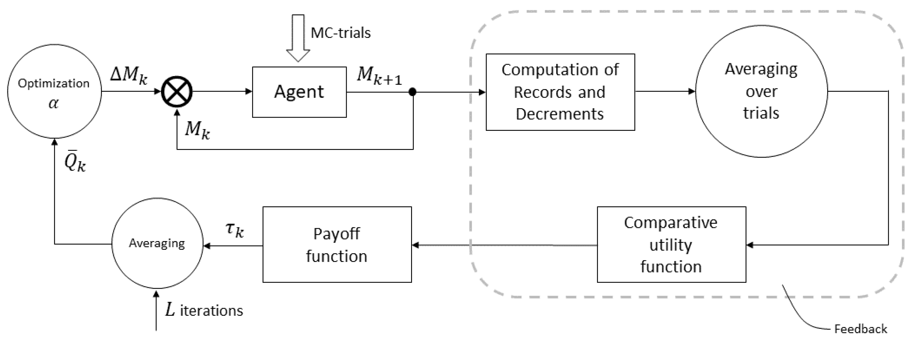
Thus, the Reinforcement module has the logical diagram shown in Figure 1. Agent is the central block of this diagram. It generates the number $M_{k+1}$ of random values on iteration $(k+1)$ as the sum of the number of random values on the previous iteration k and the optimized component $\Delta M_k$ with the parameter $\alpha$. At each iterative step, the Optimization block outputs the maximum ${\overline{Q}}_k$ of the payoffs $r_k$ accumulated over L iterations (a fixed number), which are calculated in the Payoff function block. The necessary values of the comparative utility function ${\phi }_{k,k-1}$, records $J_k^{*}$ and $J_{k-1}^{*},$ and their decrements $u_k$ and $u_{k-1}$ are calculated in the Feedback block.

Thus, the described reinforcement procedure proves the following assertion:

Let at each step of the iterative process of finding a solution to the Equations (14) and (16) a reinforcement procedure (30)–(32) is carried out, which implements the Belman optimality principle in the form (33) or (34).

Then, a strictly monotonically decreasing sequence of local records is generated:

$$J_{k_1^{*}}^{*}>J_{k_2^{*}}^{*}>\cdots >J_{k_i^{*}}^{*}>\dots ,{\mathcal{K}}^{*}=\{k_1^{*}<k_2^{*}<\cdots <k_i^{*}<\dots \}$$

(37)

Note that the sequence of local records consists of random elements but satisfies the chain of inequalities (36).

5. The Probabilistic Properties of Random Sequences Generated by the GFS-RF Algorithm

5.1. The Probabilistic Characteristics of the Packet ${𝒵}_k$

The iterative procedure is based on generating the packet ${𝒵}_k^d$ of random and independent vectors with a uniform distribution on the unit d-dimensional cube. The source of this packet is a random generator that produces on each iteration k a $(d\times M_k)$-dimensional array of independent random variables with a uniform distribution on the interval $[0,1]$.

Consider the d-dimensional unit cube $Z_{+}^d$ and the grid with step ${\eta }_k$ (23). The cube $Z_{+}^d$ is the union of the elementary cubes with side $M_k^{-q}$. We estimate the probability $P(M_k,d,q)$ that each elementary cube will contain at least one of the random vectors from the packet ${𝒵}_k^d$ generated on iteration $k.$

Lemma 1.

The probability $P(M_k,d,q)$ satisfies the upper bound

$$\begin{array}{ccc}\hfill P(M_k,d,q)& \le & 1-{(M_k^{-q/2}+1)}^d{(1-M_k^{-qd})}^{M_k^d}<\hfill \\ & <& 1-{(1-M_k^{-qd})}^{M_k^d}=P_0(M_k,d,q).\hfill \end{array}$$

(38)

where

$$P(M_k,d,q)\le \widehat{P}(M_k,d,q)\sim M_k^{q/2}exp\left(-M_k^{d(1-q/2)}\right)<1.$$

(39)

as $M_k\to \infty .$

Proof. 

Consider the partition of the interval $[0,1]$ by a grid with step ${\eta }_k\ll 1$ (23). At least one random value from $M_k={(1/\eta )}^{1/q}$ will fall into the elementary interval with the probability ${\eta }_k$. Let this grid be applied to all sides of the unit cube. Then the event A that at least one random vector from $N_k=M_k^d$ will fall into the elementary cube and has the probability ${\eta }_k^d$. Hence, the complementary event (not getting into the elementary cube) has the probability ${(1-{\eta }_k^d)}^{N_k}$.

The upper bounds on the number of elementary intervals and the number of elementary cubes are $(1+M_k^{-q/2})$ and ${(1+M_k^{-q/2})}^d,$ respectively. Therefore, the upper bound on the probability of the event A is given by

$$\widehat{P}(M_k,d,q)={(1+M_k^{-q/2})}^d{(1-{\eta }_k^d)}^{N_k}.$$

(40)

Due to the relation (25) between $M_k$ and $N_k$, we finally arrive at the upper bound (38).

For large values $M_k=x,$

$$\underset{x\to \infty }{lim}\frac{{(1-x-q)}^x}{exp(-x^{1-q})}=1,$$

which yields (39).  □

5.2. The Probabilistic Properties of the Local Record Sequence (36)

The reinforcement procedure forms the strictly monotonically decreasing sequence $J^{*}$ of local records and the sequence of their arguments ${\mathbf{z}}^{*}$. Because of their strict monotonic decrease, it is more convenient to renumber the elements by integers $1,2,\dots ,i,\dots$:

$$\begin{array}{ccc}\hfill & & {\mathcal{J}}^{*}=\{J_1^{*}>J_2^{*},>\dots ,>J_i^{*},>\dots \}\hfill \\ & & {\mathbf{z}}^{*}=\{{\mathbf{z}}_1^{*},{\mathbf{z}}_2^{*},\dots ,{\mathbf{z}}_i^{*},\dots \}.\hfill \end{array}$$

(41)

Let $\mathbb{Z}$ denote the set of points ${\mathbf{z}}^0$ corresponding to the zero value of the residual function: $J\left({\mathbf{z}}^0\right)=J^{*}=0$ (20). Due to the continuity of the function $J\left(\mathbf{z}\right)$, this set is compact.

We introduce the distance between an arbitrary point in the cube and the set $\mathbb{Z}$:

$$\varrho (\mathbf{z},\mathbb{Z})=\underset{\mathbf{y}\in \mathbb{Z}}{min}\parallel \mathbf{z}-\mathbf{y}\parallel .$$

(42)

The elements of the local record sequence are ordered but random values. Therefore, the deviation from the global record (the global minimum) takes a random value $J_i^{*}$ on each iteration. Using the assumption that the residual function (19) has a modulus of continuity $\omega (H,h)$ (22), we can formulate the following Lemma 2.

Lemma 2.

For a finite number of iterative steps i with a probability not smaller than $P_0(M_i,d,q)$ (38) and (39), we have the bilateral estimate

$$Pb\{0\le J_i^{*}-J^{*}\le \omega (H,h_i)\}>P_0(M_i,d,q),$$

(43)

where $\omega (H,h_i)$ denotes the modulus of continuity of the function $J\left(\mathbf{z}\right)$ (22), and $h_i=\frac{\sqrt{d}}{2}{M}_i^{-q}$.

Proof. 

Consider the random points generated on iteration i among them, let $\widehat{\mathbf{z}}$ be the closest one to the set $\mathbb{Z}$ in terms of the distance (42).

At least one of these points will fall with a probability not smaller than $P_0(M_i,d,q)$ into each elementary cube with side $M_i^{-q};$ see Lemma 1. Hence,

$$h_i=\parallel \widehat{\mathbf{z}}-{\mathbf{z}}^0\parallel \le M_i^{-q}\frac{\sqrt{d}}{2}.$$

(44)

This happens if the point ${\mathbf{z}}^0$ corresponding to the zero value of the residual function is in the center of the elementary cube with side $M_i^{-q}$ and its nearest random points are in the cube vertices so that each cube contains at least one random point.

By the Hölder condition (22), we have

$$0\le J\left(\widehat{\mathbf{z}}\right)-J^{*}\le \omega \left(h_i\right).$$

(45)

On the other hand,

$$J^{*}=J\left({\mathbf{z}}^0\right)=\underset{\mathbf{z}\in Z^d}{min}J\left(\mathbf{z}\right)\le \underset{s,1\le s\le i}{min}J\left({\mathbf{z}}^s\right)=J_i^{*}\le J\left(\widehat{\mathbf{z}}\right).$$

(46)

This chain of inequalities implies

$$0\le J_i^{*}-J^{*}\le J\left(\widehat{\mathbf{z}}\right)-J^{*}.$$

(47)

From (45) and (47) it follows that

$$0\le J_i^{*}-J^{*}\le \omega (H,h_i)$$

(48)

with a probability not smaller than $P_0(M_i,d,q)$.  □

Inequality (48) provides an upper bound on the deviation from the zero value of the residual function on each iteration obtained after the reinforcement procedure and a lower bound on the probability $P_0(M_i,d,q)$ (38) of its realization. The upper bound is the value of the modulus of continuity of the function J on these iterations. In other words, according to (22),

$$\omega (H,h_i)\le H{h}_i^s=H{\left({\eta }_i\frac{\sqrt{d}}{2}\right)}^s=H{\left(M_i^{-q}\frac{\sqrt{d}}{2}\right)}^s.$$

(49)

With the notations

$$\begin{array}{ccc}\hfill & & D=H{\left(\frac{\sqrt{d}}{2}\right)}^s,p=sq,\hfill \\ & & r_i(D,p)=D{M}_i^{-p}.\hfill \end{array}$$

(50)

we arrive at a very useful probabilistic form of inequality (49):

$$P\{0\le J_i^{*}-J^{*}\le r_i(D,p)\}\ge P_0(M_i,d,q).$$

(51)

It gives a lower bound on the probability that the current record will fall into the neighborhood of the global minimum as well as determines its size.

5.3. The Size of the Neighborhood of the Global Minimum

Consider a sequence of decrements on a finite number of iterations k:

$$u_k=J_k^{*}-J_{k-1}^{*}<0,\forall k=1,2,\dots$$

(52)

We represent the decrements as

$$|u_k|=|(J_k^{*}-J^{*})-(J_{k-1}^{*}-J^{*})|.$$

(53)

Due to (51)

$$|u_k| \le |(J_{k-1}^{*}-J^{*})| - |(J_k^{*}-J^{*})| \le D\left(M_{k-1}^{-p}-M_k^{-p}\right)=D{M}_k^{-p}{\beta }_k\left(p\right)\le D{M}_k^{-p},$$

(54)

where, due to (33)

$${\beta }_k\left(p\right)=1-{\left(\frac{M_{k-1}}{M_k}\right)}^{-p},{\beta }_k\left(p\right)\in [0,1],\forall p,k.$$

(55)

The boundary value of the modulus of continuity of the decrement for k iterations is

$$u_k^{*}=D{M}_k^{-p},$$

(56)

or, in the logarithmic scale,

$$log{u}_k^{*}=logD-plog{M}_k.$$

(57)

Thus, we have a linear dependence with unknown parameters $logD$ and p, which are related to the parameters of the modulus of continuity (22). Their values can be estimated using the available data on $log{u}_k^{*}$ and $log{M}_k$ by the least squares method. The parameters D and p determine the size of the neighborhood of the global minimum and the probability of reaching it (50) and (51).

Remark 2.

The upper bound (54) is very conservative: it focuses on estimating the elements of the local record sequence and neglects an essential feature of the decrement sequence. In the latter, the number of random values on iteration $(k+1)$ changes compared to iteration k due to the reinforcement procedure (33) and (34).

This feature is reflected in the expression for the decrement boundary value:

$$u_k^{*}=D{M}_k^{-p}{\beta }_k\left(p\right),{\beta }_k\left(p\right)=1-{\left(\frac{1}{{\tilde{M}}_k}\right)}^p,$$

(58)

where the reinforcement procedure (34) generates the values

$${\tilde{M}}_k=arg\underset{M_k}{max}{\overline{Q}}_k\left(M_k\right).$$

(59)

By analogy with (57), we obtain

$$log{u}_k^{*}=logD-plog{M}_k+log{\beta }_k({\tilde{M}}_k,p).$$

(60)

This dependence still has two parameters, D and p, but the data include $log{u}_k^{*}, M_k,$ and $\widetilde{M_k}$ additionally generated by the reinforcement procedure. The dependence (60) is nonlinear. Its parameters can be restored using the least squares method as well. As in the previous case, however, there is no guarantee of obtaining the optimal result.

6. The Convergence of the GFS-RF Algorithm to the Global Minimum

The reinforcement procedure (30)–(33), combined with the selection of local records, makes their sequence the property of a strictly monotonic decrease (37), accompanied by a sequence of decrements with negative elements (36). Based on them, we can formulate the following Theorem 1.

Theorem 1.

Let the following conditions be satisfied for a finite number of iterations equal to k:

(𝚊). inequalities (37) and (36) are true;

(б). function $J\left(\mathit{z}\right)$ is of Hoelder type with parameters of mudulus of continuity $(H^{*},h_k^{*})$ which are estimated by (57);

(b). area ${\mathcal{R}}_k^{*}$ of the existence of global extrema is as follows:

$${\mathcal{R}}_k^{*}=\{J:|J_k^{*}-J^{*}| \le r_k(D,p)\},$$

(61)

where

$$r_k(D,p)=D{M}_k^{-p}.$$

(62)

Then the sequence of local records ${\mathcal{J}}_k^{*}=\{J_1^{*}>J_2^{*},>\cdots >J_k^{*}\}$ at k iterations achieve the area ${\mathcal{R}}_k^{*}$ with probability not less than

$$P_0(M_k,d,q)=1-{\left(1-M_k^{dq}\right)}^{M_k^d},$$

(63)

and at high values of $M_k$

$$P_0(M_k,d,q)\sim M_k^{q/2}exp\left(-M_k^{d(1-q/2)}\right).$$

(64)

Proof. 

The proof follows from Lemmas 1 and 2 and the estimate (51).  □

7. Discussion and Conclusions

The concept and computational procedure of Randomized Machine Learning proposed in [22] turned out to be very useful in terms of inaccurate data estimation probability distributions, and also an effective computer technique for solving many applied problems [24]. The modules of this procedure have been applied to practical problems of the randomized forecasting of World population [32], electrical load in the power systems [33], the evolution of the thermokarst lakes in the Arctic zone [34], randomized classification of the objects [35,36]. In these works, we used public datasets of the UN [37], and [38]. However, its practical application is associated with solving a very difficult problem of finding solutions to a specific system of nonlinear equations in which only the values of the functions included in it are available.

In this paper, we propose to use the idea of reinforcement to give adaptive properties to computational algorithms. A problem-oriented reinforcement procedure based on the agent-based approach is proposed, in which the agent generates a strategy in terms of the optimal number of random numbers generated at each step of the iterative process. As a utility function, the exponential comparative utility function is used, which depends on the average decrements of local records achieved at each main iteration. An important role in the reinforcement procedure is played by the payoff function, which generates “penalties” on the values of the utility function. Optimization of the agent’s strategy is carried out using R. Belman’s principle of optimality. As a result of applying the reinforcement procedure, the dimensions of the neighborhood of the global minimum of the quadratic residual function and the probability of its achievement with a finite number of iterations are determined.

References

- Rosenblatt, F. Principles of Neirodynamic: Perceptrons and the Theory of Brain Mechanisms; Spartan Books: Washington, DC, USA, 1962. [Google Scholar]
- Gelfand, I.M.; Pyatetskij-Shapiro, I.I.; Tsetlin, M.L. Certain Classes of Games and Automata Games. Sov. Phys. Dokl. 1964, 8, 964–966. [Google Scholar]
- Wasserman, P.D. Neural Computing: Theory and Practice; Van Nostrand Reinhold Co.: New York, NY, USA, 1992. [Google Scholar]
- Kohonen, T. Self-Organizing Maps; Springer: Berlin/Heidelberg, Germany, 1995. [Google Scholar]
- Mnih, V.; Kavukcuoglu, K.; Silver, D.; Rusu, A.A.; Veness, J.; Bellemare, M.G.; Graves, A.; Riedmiller, M.; Fidjeland, A. Human-level Control through Deep Reinforcement Learning. Nature 2015, 518, 529–533. [Google Scholar] [CrossRef] [PubMed]
- Sutton, R.S.; Barto, A.G. Introduction to Reinforcement Learning; MIT Press: Cambridge, UK, 1998. [Google Scholar]
- Russel, S.J.; Norvig, P. Artificial Intelligence: A Modern Approach, 3rd ed.; Prentice Hall: Upper Saddle River, NJ, USA, 2010. [Google Scholar]
- van Hasselt, H. Reinforcement Learning in Continuous State and Action Spaces. In Reinforcement Learning: State-of-the-Art; Wiering, M., van Otterio, M., Eds.; Springer Sciences & Business Media: Berlin/Heidelberg, Germany, 2012; pp. 207–257. [Google Scholar]
- Kropotov, D.; Bobrov, E.; Ivanov, S.; Temirchev, P. Reinforcement Learning Textbook. arXiv 2022, arXiv:2201.09746v1. (In Russian) [Google Scholar]
- Bozinovski, S. Crossbar Adaptive Array: The First Connectionist Network That Solved the Delayed Reinforcement Learning Problem. In Artificial Neural Nets and Genetic Algorithms; Dobnikar, A., Steele, N.C., Pearson, D.W., Albrecht, R.F., Eds.; Springer Science & Business Media: Berlin/Heidelberg, Germany, 1999; pp. 320–325. [Google Scholar]
- Watkins, C.; Dayan, P. Q-learning. Mach. Learn. 1992, 8, 279–292. [Google Scholar] [CrossRef]
- van Hasselt, H.; Guez, A.; Silver, D. Deep Reinforcement Learning with Double Q-learning. In Proceedings of the 13th AAAI Conference on Artificial Intelligence, Phoenix, AZ, USA, 12–17 February 2016; pp. 2094–2100. [Google Scholar]
- Bellman, R. Dynamic Programming; Princeton University Press: Princeton, NJ, USA, 1957. [Google Scholar]
- Robbins, H.; Monro, S. A Stochastic Approximation Method. Ann. Math. Stat. 1951, 22, 400–407. [Google Scholar] [CrossRef]
- Spong, M.W.; Hutchinson, S.; Vidyasagar, M. Robot Modeling and Control; Wiley: Hoboken, NJ, USA, 2005. [Google Scholar]
- Koshmanova, N.P.; Pavlovsky, V.E.; Trifonov, D.S. Reinforcement Learning for Manipulator Control. Rus. J. Nonlin. Dyn. 2012, 8, 689–704. (In Russian) [Google Scholar] [CrossRef]
- Fu, Y.; Jha, D.K.; Zhang, Z.; Yuan, Z.; Ray, A. Neural Network-Based Learning from Demonstration of an Autonomous Ground Robot. Machines 2019, 7, 24. [Google Scholar] [CrossRef]
- Nikitin, P.V.; Gorokhova, R.I.; Korchagin, S.A.; Krasnikov, V.S. Applying Deep Reinforcement Learning to Algorithmic Trading. Mod. Inf. Technol. IT-Educ. 2020, 16, 510–517. (In Russian) [Google Scholar]
- Esfahani, N.; Malek, S. Uncertainty in Self-Adaptive Software Systems. In Software Engineering for Self-Adaptive Systems II; de Lemos, R., Giese, H., Müller, H.A., Shaw, M., Eds.; Lecture Notes in Computer Science Book Series; Springer: Berlin/Heidelberg, Germany, 2013; pp. 214–238. [Google Scholar] [CrossRef]
- Ghezzi, C.; Salvaneschi, G.; Pradella, M. ContextErlang. Sci. Comput. Program. 2015, 102, 20–43. [Google Scholar] [CrossRef]
- Bencvoma, N.; Belaggoun, A. Supporting Decision-Making for Soft-Adaptive Systems: From Goal Models to Dynamic Decision Network. In Requirements Engineering: Foundation for Software Quality, proceedings of the 19th International Working Conference, REFSQ 2013, Essen, Germany, 8–11 April 2013; Springer: Berlin/Heidelberg, Germany, 2013; pp. 221–236. [Google Scholar]
- Popkov, Y.S.; Popkov, A.Y. New Nethod of Entropy-Robust Estimation for Randomized Models under Limited Data. Entropy 2014, 16, 675–698. [Google Scholar] [CrossRef]
- Popkov, Y.S.; Dubnov, Y.A.; Popkov, A.Y. Randomized Machine Learning: Statement, Solution, Applications. In Proceedings of the IEEE 8th International Conference on Intelligent Systems, Sofia, Bulgaria, 4–6 September 2016; pp. 27–39. [Google Scholar]
- Popkov, Y.S.; Popkov, A.Y.; Dubnov, Y.A. Entropy Randomization in Machine Learning; CRC Press: Boca Raton, FL, USA, 2023. [Google Scholar]
- Darkhovskii, B.S.; Popkov, A.Y.; Popkov, Y.S. Monte Carlo Method of Batch Iterations: Probabilistic Characteristics. Autom. Remote Control 2015, 76, 775–784. [Google Scholar] [CrossRef]
- Popkov, A.Y.; Darkhovskii, B.S.; Popkov, Y.S. Iterative MC-Algorithm to Solve the Global Optimization Problems. Autom. Remote Control 2017, 78, 261–275. [Google Scholar] [CrossRef]
- Avellaneda, M. Minimum-Relative-Entropy Calibration of Asset-Pricing Models. Int. J. Theor. Appl. Financ. 1998, 1, 447–472. [Google Scholar] [CrossRef]
- Vine, S. Options: Trading Strategy and Risk Management, 1st ed.; Wiley: Hoboken, NJ, USA, 2005. [Google Scholar]
- Magnus, J.R.; Neudecker, H. Matrix Differential Calculus (with Applications in Statistics and Econometrics); John Wiley and Sons: New York, NY, USA, 1999. [Google Scholar]
- von Neumann, J.; Morgenstern, O. Theory of Games and Economic Behavior; Princeton Univiversity Press: Princeton, NJ, USA, 1944. [Google Scholar]
- Fishburn, P.C. Utility Theory for Decision Making; Wiley: New York, NY, USA, 1970. [Google Scholar]
- Popkov, Y.S.; Dubnov, Y.A.; Popkov, A.Y. New Method of Randomized Forecasting Using Entropy-Robust Estimation: Application to the World Population Prediction. Mathematics 2016, 4, 16. [Google Scholar] [CrossRef]
- Popkov, Y.S.; Popkov, A.Y.; Dubnov, Y.A.; Solomatine, D. Entropy-Randomized Forecasting of Stochastic Dynamic Regression Models. Mathematics 2020, 8, 1119. [Google Scholar] [CrossRef]
- Dubnov, Y.A.; Popkov, A.Y.; Polyschuk, V.Y.; Sokol, E.A.; Melnikov, A.V.; Polyschuk, Y.M.; Popkov, Y.S. Randomized Machine Learning to Forecast the Evolution of Thermokarst Lakes in Permafrost Zones. Autom. Remote Control 2023, 84, 56–70. [Google Scholar] [CrossRef]
- Popkov, Y.S.; Volkovich, Z.; Dubnov, Y.A. Entropy “2”-Soft Classification of Objects. Entropy 2017, 19, 178. [Google Scholar] [CrossRef]
- Dubnov, Y.A. Entropy-Based Estimation in Classification Problems. Autom. Remote Control 2019, 80, 502–512. [Google Scholar] [CrossRef]
- UNdata—A World of Information. Available online: https://data.un.org (accessed on 17 August 2023).
- Hong, T.; Prinson, P.; Fan, S.; Zareipour, H.; Triccoli, A.; Hyndman, R.J. Probabilistic Energy Forecasting: Global Energy Forecasting Competition 2014 and Beyond. Int. J. Forecast. 2016, 32, 896–913. [Google Scholar] [CrossRef]
Figure 1.
Logical diagram of the Reinforcement module.
Disclaimer/Publisher’s Note: The statements, opinions and data contained in all publications are solely those of the individual author(s) and contributor(s) and not of MDPI and/or the editor(s). MDPI and/or the editor(s) disclaim responsibility for any injury to people or property resulting from any ideas, methods, instructions or products referred to in the content. |
© 2023 by the authors. Licensee MDPI, Basel, Switzerland. This article is an open access article distributed under the terms and conditions of the Creative Commons Attribution (CC BY) license (https://creativecommons.org/licenses/by/4.0/).
Share and Cite
MDPI and ACS Style
Popkov, Y.S.; Dubnov, Y.A.; Popkov, A.Y. Reinforcement Procedure for Randomized Machine Learning. Mathematics 2023, 11, 3651. https://doi.org/10.3390/math11173651
AMA Style
Popkov YS, Dubnov YA, Popkov AY. Reinforcement Procedure for Randomized Machine Learning. Mathematics. 2023; 11(17):3651. https://doi.org/10.3390/math11173651
Chicago/Turabian StylePopkov, Yuri S., Yuri A. Dubnov, and Alexey Yu. Popkov. 2023. "Reinforcement Procedure for Randomized Machine Learning" Mathematics 11, no. 17: 3651. https://doi.org/10.3390/math11173651
Note that from the first issue of 2016, this journal uses article numbers instead of page numbers. See further details here.