Spatio-Temporal Coherence of mmWave/THz Channel Characteristics and Their Forecasting Using Video Frame Prediction Techniques

Abstract

Channel state information in millimeter wave (mmWave) and terahertz (THz) communications systems is vital for various tasks ranging from planning the optimal locations of BSs to efficient beam tracking mechanisms to handover design. Due to the use of large-scale phased antenna arrays and high sensitivity to environmental geometry and materials, precise propagation models for these bands are obtained via ray-tracing modeling. However, the propagation conditions in mmWave/THz systems may theoretically change at very small distances, that is, 1 mm–1 $\mathsf{\mu }$m, which requires extreme computational effort for modeling. In this paper, we first will assess the effective correlation distances in mmWave/THz systems for different outdoor scenarios, user mobility patterns, and line-of-sight (LoS) and non-LoS (nLoS) conditions. As the metrics of interest, we utilize the angle of arrival/departure (AoA/AoD) and path loss of the first few strongest rays. Then, to reduce the computational efforts required for the ray-tracing procedure, we propose a methodology for the extrapolation and interpolation of these metrics based on the convolutional long short-term memory (ConvLSTM) model. The proposed methodology is based on a special representation of the channel state information in a form suitable for state-of-the-art video enhancement machine learning (ML) techniques, which allows for the use of their powerful prediction capabilities. To assess the prediction performance of the ConvLSTM model, we utilize precision and recall as the main metrics of interest. Our numerical results demonstrate that the channel state correlation in AoA/AoD parameters is preserved up until approximately 0.3–0.6 m, which is 300–600 times larger than the wavelength at 300 GHz. The use of a ConvLSTM model allows us to accurately predict AoA and AoD angles up to the 0.6 m distance with AoA being characterized by a higher mean squared error (MSE). Our results can be utilized to speed up ray-tracing simulations by selecting the grid step size, resulting in the desired trade-off between modeling accuracy and computational time. Additionally, it can also be utilized to improve beam tracking in mmWave/THz systems via a selection of the time step between beam realignment procedures.

1. Introduction

With the advent of 5G new radio (NR) systems, operators promise to deliver radically higher user data rates at the access interface, which will enable new applications such as holographic communications, augmented/virtual reality (AR/VR), and high-resolution streaming [1]. At the same time, the research community is already discussing 6G systems, which will further enhance system throughput and diversify the service offerings [2,3].

The fulfillment of the above-named promises is conditioned on the use of millimeter wave (mmWave) and terahertz (THz) frequency bands, both characterized by extremely short wavelengths. Due to the limitation of the effective antenna apertures, such systems must utilize large-scale phased antenna arrays operating in the beamforming regime to improve the coverage area [4,5,6,7]. Precise knowledge of the propagation conditions at mmWave/THz frequencies is required at many stages of the system’s design [8]. At the network planning stage, optimal locations of base stations (BS) maximizing the coverage area need to be determined [9]. Further, utilizing the beamforming regime of antenna arrays, one needs to develop an efficient beam tracking mechanism [10]. However, the use of such arrays as well as complex propagation effects such as reflection, diffraction, and scattering leads requires advanced channel models to predict channel conditions.

Ray tracing is conventionally utilized to develop accurate propagation models. By using either image or ray-launching methods, they allow precise information to be obtained about the received signal strength at any given point by taking into account the geometry of the propagation environment and surrounding materials. However, ray tracing is an inherently resource-consuming procedure, even at lower frequencies, and the use of mmWave/THz bands in 5G/6G cellular systems requires much detailed resolution because the channel state parameters may change at distances comparable to the wavelength. Thus, obtaining detailed propagation maps is an extremely time-consuming procedure.

In light of the aforementioned limitations, several studies have suggested different speed-up techniques for ray-tracing simulations; see Section 2 for a detailed review. However, all those either explicitly or implicitly assume that a correlation between channel state parameters is preserved across distances larger than the wavelength. While this may indeed be true for some propagation conditions, to the best of the authors’ knowledge, there has been no detailed investigation into the effective correlation distances in typical propagation environments. Furthermore, some studies aiming to improve the beam tracking procedures for mmWave/THz systems, also implicitly assume this property.

In this paper, we first utilize a ray-tracing tool to quantitatively evaluate the effective correlation distance between channel state parameters for typical outdoor propagation environments, different user mobility patterns, and line-of-sight (LoS) and non-LoS (nLoS) conditions. As metrics of interest, we utilize the angle of arrival/departure (AoA/AoD) and path loss over the first few strongest paths. Having this information, we then propose a methodology to further enhance the considered distance between ray-tracing points. The methodology relies on representing the channel state parameters as frames similar to video frames and applying state-of-the-art techniques for interpolation and extrapolation.

The main contributions of our study are as follows:

• Correlational properties between channel state parameters in mmWave/THz systems are in the order of at least 30–60 cm, with AoD being characterized by much stronger dependence as compared to AoA, which is 300–600 times higher than the wavelength at 300 GHz;
• Representation of the channel state parameters in a form convenient for modern state-of-the-art video frame interpolation and prediction techniques;
• ML prediction results, showing that reliable prediction accuracy of AoA and AoD angles is feasible up to 60 cm distance, with AoA being characterized by a higher mean squared error (MSE).

The rest of the paper is organized as follows. First, in Section 2, we overview the related work. Further, in Section 3, by utilizing a ray-tracing tool, we quantify the correlation properties of the main channel parameters. ML-based mechanisms for channel state parameter prediction are introduced in Section 4, while their evaluation is provided in Section 4.4. Conclusions are drawn in the last section.

2. Related Work

In this section, we overview the related work. We start with techniques proposed for speeding up ray-tracing channel modeling. Further, we briefly overview the research on beam-tracking mechanisms, where channel state information produced via ray tracing is heavily utilized.

2.1. Speeding-Up Techniques for Ray-Tracing Modeling

Ray-tracing-based channel models are the most efficient for mmWave/THz systems, but involve extremely long computations, which grow substantially as the carrier frequency increases. Many efficient ray-tracing models have been proposed in the literature. One of the popular approaches is based on reducing the number of edges and planes of the environment elements on which ray-tracing will be performed. The article [11] presented a method based on the visibility graph: a tree-like list of elements with which rays can interact on their way from the transmitter to the receiver. The authors of [12] also use the visibility graph, but only consider beams that are in the 18 dB dynamic range, based on ITU recommendations. As a result, they were able to increase the simulation speed from 2 to 4 times, depending on the initial data. Another method based on the visibility graph was proposed in [13], where the authors also took into account a transformation of two dimensions (2D) to three dimensions (3D) using Fermat’s principle. In addition, the authors analyzed the impact of the number of reflections taken into account on the accuracy of the calculations. The proposed method requires additional preprocessing time, as they need to find all the possible ray propagation paths before simulation. However, they can significantly speed up the ray-tracing procedure without losing accuracy. Specifically, the authors managed to reduce the simulation time for 1651 receivers from several hours to several seconds after preprocessing.

A binary space-partitioning method (BSP) was proposed by the authors in [14]. This method, in contrast to the graph of visibility, divides not the elements of the space but the space itself, which led to a decrease in the load on the processor by about 60%. A similar approach was employed in [15], where the authors used a visibility table. The authors provided an efficient algorithm for a mobile transmitter; the model uses a precomputed visibility table that makes it easy to determine visible walls and edges, which can accelerate preprocessing time by up to 90%. In [16], a space-partitioning method was proposed to model ray tracing efficiently. The method is based on the division of space into smaller ones and the distribution of objects according to the areas where they are located. The main idea of the method is to find the subspace into which the ray from the current subspace will enter using the given direction and slope of the ray. This approach made it possible to achieve a 14% reduction in CPU time compared to traditional visibility methods. Another approach divides the space into a mesh of triangles to simplify the modeling of the interaction of the beam with the elements of the environment [17]. After division, groups of rays are collected into frustums that are further utilized for modeling.

Another approach to speed up ray tracing is based on data simplification that does not have a strong impact on the results. For example, the authors in [18] aimed to improve ray-tracing performance by optimizing the object database. The article proposes to reduce the number of objects that are not involved in ray tracing, as well as to simplify the geometric shape of buildings, thereby significantly reducing the computation time without a noticeable impact on accuracy. Based on the results of the experiments, the authors managed to reduce the simulation time by a factor of more than 2. The article [19] proposed a method for post-processing ray-tracing data modeled in urban environments. It was proposed to combine rays that have undergone the same interaction into ray entities, which made it possible to reduce the load on memory by 11–12 times.

Unfortunately, many of the aforementioned methods lose their effectiveness with the increase in carrier frequency, especially in mmWave and THz bands. At these frequencies, machine learning (ML) is often considered to speed up ray-tracing simulations. The authors in [20] proposed a way to reduce the number of rays launched by the “shooting and bouncing” (SBR) method. The latter involves the spherical launch of rays from the transmitter in all possible directions with a fixed value of the angle between the rays. Using a neural network, it was possible to reduce the number of launched rays by predicting intermediate rays. As a result, it was possible to reduce simulation time by 80% and memory consumption by 70%. It should be noted, however, that the proposed method has not been tested using high frequencies and simulations in urban environments. In a recent study [21], the authors compared several neural networks with the aim of increasing the resolution of radio channel simulation using ray-tracing. In continuation of their previous work, the authors of [22] presented a method for accelerating ray tracing when simulating mobile channels in urban environments in 5G mmWave systems using methods for combining similar rays into clusters. Channel characteristics were predicted at intermediate points of the mobile receiver trajectory. Experiments have shown that the proposed approach allows us to accurately predict the received power compared to the traditional interpolation method.

Most of the presented approaches are based on a simplification of the environment or a transition from 3D to 2D. It is also worth noting that most methods were aimed at indoor scenarios and may not be effective in outdoor deployments. Finally, most of the ML-based studies did not characterize the environment statistically assessing the potential for interpolation and extrapolation techniques.

2.2. Efficient Beam Tracking in mmWave/THz Systems

The problem of fast ray tracing is tightly related to the problem of efficient beam tracking in mmWave/THz systems [23]. Indeed, in the former case, one wants to interpolate or extrapolate the received signal strength based on the limited number of measurements, e.g., launched rays. In beam tracking, the core problem is to determine the current direction to BS/UE (User Equipment) based on the minimal number of measurements.

Numerous ML-based beam tracking methods have been proposed in the past to provide high tracking accuracy continuously in various scenarios. The main two advantages of ML approaches are the ability to capture the dynamics of the channel and environment. The authors in [24] proposed the beam-training approach to acquire channel state information and select the optimal beam so that a target communication quality can be maintained. In [25], the authors proposed a prediction model based on a long short-term memory (LSTM) network. The model utilizes previously measured channel state information (CSI) samples to estimate the channel. The authors in [26] proposed a deep neural network (DNN)-based approach to determine the hidden relation between the received training signal and the mmWave channel state. The authors of [27] proposed a data-driven beam-tracking approach to find the beamforming/combining vectors. The proposed scheme searches all the beamforming and combining vector configurations to achieve the target quality of service (QoS) by minimizing the tracking error through a series of equivalent local dynamic linearizations. The authors showed that the proposed algorithm can achieve reliable tracking performance with a much shorter alignment time as compared to traditional schemes. In [28], the authors proposed to combine a deep learning-based tracking algorithm (deep sort) and beamforming in 5G NR to predict and track the UE’s location. They showed that the predicted UE location can help in focusing data toward their location without any feedback mechanism. Thus, reducing the feedback improves the network efficiency.

Similarly to the task of speeding up the ray-tracing simulations, most of the studies addressing the problem of efficiency did not carry out statistical studies to assess the potential for inter- and extrapolation of consecutive signals to reduce the scanning space. The goal of our work is to assess the correlation between the signals to accelerate the ray-tracing simulations and beam-tracking process.

3. Data Analysis

In this section, we analyze dependencies in path loss data in different typical outdoor deployments and channel states. We start this section by describing the utilized ray-tracing tool and experimental setup, and then proceed with the data representation and statistical data analysis.

3.1. Tools

Numerous software packages allow for the simulation of the propagation of radio waves. Each product is characterized by a different set of features and has both advantages and shortcomings. Next, we briefly overview the popular software used in scientific and engineering research.

MATLAB Communication toolbox [29]. It is a built-in library of the popular MATLAB software. This software offers a variety of possibilities for ray-tracing modeling. Here, one can use the mapping method or the SBR method and set basic parameters such as the location of the receiver and transmitter, the size of their antenna arrays, the carrier frequency, the parameters of materials, weather conditions, etc. Also, using this module, one can calculate all the main parameters of the simulated system, such as propagation losses, received power at the UE, BS coverage map, etc. As an environment, one can use 3D street maps in .osm format, which can be downloaded from the OpenStreetMap [30] service, as well as 3D indoor models in .stl format. One of the main advantages of this tool is compatibility with all popular operating systems. The shortcomings include the lack of the ability to simulate ray tracing in combination with mobile objects, the limited choice of materials for objects, as well as the inability to create a 3D environment directly via the software interface.

Wireless Insite [31]. This software includes one of the largest feature sets and is the most commonly used in scientific work. The SBR method is used to simulate ray-tracing. This software allows for the incorporation of various 3D environments, adjusting the materials of objects, and calculating and setting the entire range of parameters, such as the location of receivers and transmitters, carrier frequency, power, propagation loss, etc. It is possible to create a 3D environment through the program interface. The shortcomings include the inability to simulate ray tracing in combination with mobile objects, and the inability to select a ray-tracing method. This software is distributed on a commercial basis and is compatible with the Windows operating system only.

Ansys HFSS [32]. Ansys software is extremely powerful in modeling radio wave propagation. The main advantage is the ability to model objects with complex geometry and materials, as well as simulate scenarios with mobile objects. In addition to the standard features that are implemented in MATLAB Communication Toolbox and Wireless InSite, there is the possibility for modeling extended physics of diffraction effects, the possibility of accelerating the performance of modeling, and an advanced system for visualizing the propagation of rays. Similarly to Wireless InSite, Ansys HFSS is a commercial tool.

WinProp [33]. WinProp is another fairly popular software for ray-tracing simulations. It has a set of features similar to the Wireless Insite and MATLAB Communication toolbox and is widely used in the scientific community. Among the advantages, we note the built-in graphical user interface (GUI) capable of creating both urban outdoor environments and various indoor premises. Also, the advantages include proprietary algorithms for accelerating ray tracing for image methods and SBR, as well as the ability to apply ray tracing to mobile objects. Among the shortcomings are distribution on a commercial basis, limited visualization capabilities, the inability to model complex objects, and compatibility only with the Windows operating system.

In our study, we utilize the MATLAB Communication toolbox, as it allows for modifications of the ray-tracing mechanisms, a detailed configuration of the considered scenarios, utilization of user-defined output data formatting, and built-in statistical functions.

3.2. Experimental Setup and Metrics

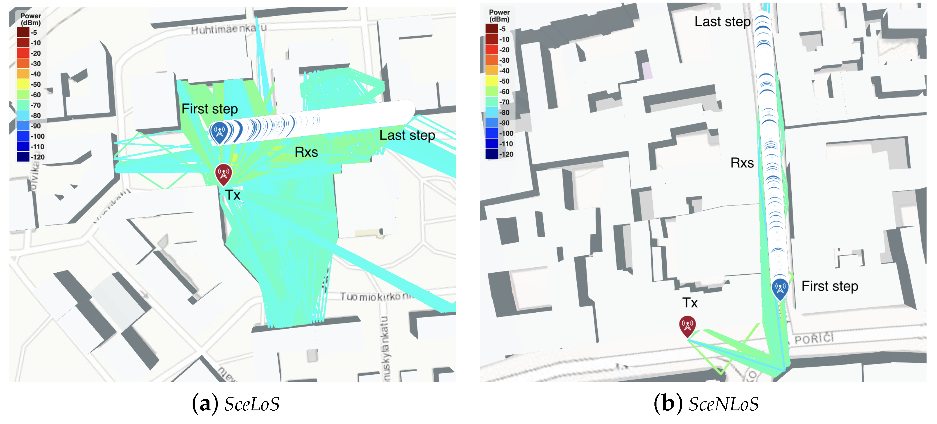
We consider an urban deployment where a receiver (Rx) moves along a street and the transmitter (Tx) is fixed at a certain height. We explore different LoS/nLoS conditions of the channel between Tx and Rx by considering the following three scenarios:

• SceLoS: Rx moves in a straight line in the line of sight of Tx (Figure 1a),
• SceNLoS: Rx moves in a straight line not in the line of sight of Tx (Figure 1b),
• SceTurn: Rx makes a 90-degree turn moving from LoS to nLoS of Tx (Figure 2).

Before performing the ray-tracing modeling, we divide a considered Rx trajectory T into S segments of length $\Delta s$. A receiver, Rx${}_s$, is then placed at the starting point of each segment, and ray-tracing between Tx and Rx${}_s$ is performed separately for each $s=1,\cdots ,S$. In what follows, we refer to the position of Rx${}_s$ as step s of trajectory T, and to $\Delta s$ as the step size. Note that depending on the considered application—speeding-up ray-tracing simulations or beam tracking—the step size may correspond to the size of the grid utilized for beam tracking or time intervals between beam-tracking events.

Our task is to determine the similarity in the data between steps of the Rx’s trajectory. We focus on three parameters of interest: (i) angle of arrival (AoA), (ii) angle of departure (AoD), and (iii) path loss. For each step $s=1,\cdots ,S$ of a trajectory T, the ray-tracing procedure yields a set ${\mathcal{I}}_T\left(s\right)=\{i_{s,1},i_{s,2},\cdots \}$ of rays that have reached Rx${}_s$ within the preset number of reflections. Because we usually consider one trajectory at a time, index T is omitted whenever practical. We denote the cardinality of the set by $I\left(s\right)=\left|\mathcal{I}\right(s\left)\right|\ge 0$ and index the rays therein according to their path loss so that ray $i_{s,1}$ is the strongest. For each ray $i_{s,j}\in \mathcal{I}\left(s\right)$, we collect (i) its azimuth and elevation angles of arrival, which we denote by ${\phi }_{s,j}^{\mathrm{AoA}}$ and ${\theta }_{s,j}^{\mathrm{AoA}}$, respectively; (ii) its azimuth and elevation angles of departure, denoted by ${\phi }_{s,j}^{\mathrm{AoD}}$ and ${\theta }_{s,j}^{\mathrm{AoD}}$, respectively; and (iii) the path loss in dB, denoted by $P{L}_{s,j}$. Thus, the elements of $\mathcal{I}\left(s\right)$ are tuples of the form $i_{s,j}=\left({\phi }_{s,j}^{\mathrm{AoA}},{\theta }_{s,j}^{\mathrm{AoA}},{\phi }_{s,j}^{\mathrm{AoD}},{\theta }_{s,j}^{\mathrm{AoD}},P{L}_{s,j}\right)$. However, it can be practical to conduct analysis from the perspective of Tx using AoD and from the perspective of Rx using AoA separately. Therefore, we split the previous tuples and consider two sets of triplets:

$$\begin{array}{cc}\hfill & {\mathcal{I}}^{\mathrm{AoA}}\left(s\right)=\left\{\left({\phi }_{s,j}^{\mathrm{AoA}},{\theta }_{s,j}^{\mathrm{AoA}},P{L}_{s,j}\right):\left({\phi }_{s,j}^{\mathrm{AoA}},{\theta }_{s,j}^{\mathrm{AoA}},{\phi }_{s,j}^{\mathrm{AoD}},{\theta }_{s,j}^{\mathrm{AoD}},P{L}_{s,j}\right)\in \mathcal{I}\left(s\right)\right\},\hfill \\ \hfill & {\mathcal{I}}^{\mathrm{AoD}}\left(s\right)=\left\{\left({\phi }_{s,j}^{\mathrm{AoD}},{\theta }_{s,j}^{\mathrm{AoD}},P{L}_{s,j}\right):\left({\phi }_{s,j}^{\mathrm{AoA}},{\theta }_{s,j}^{\mathrm{AoA}},{\phi }_{s,j}^{\mathrm{AoD}},{\theta }_{s,j}^{\mathrm{AoD}},P{L}_{s,j}\right)\in \mathcal{I}\left(s\right)\right\}.\hfill \end{array}$$

(1)

3.3. Clustering and Data Representation

Radio channel simulation between Tx and Rx using ray tracing can result in several hundreds, and even thousands, of rays with similar characteristics. Ray clustering [22] involving grouping similar beams into groups called clusters is often used in the literature [22] and standards [34]. In this work, we also employ this approach and group together beams that have close AoA or AoD values.

As mentioned previously, AoA and AoD are characterized by two angles—azimuth and elevation—which are measured in degrees and vary in the ranges $(-180,180]$ and $[-90,90]$, respectively. To benefit from the powerful ML techniques developed for video processing, and also to perform clustering, we represent each data point, i.e., a set $\mathcal{I}\left(s\right)$, in the form of two images or video-like frames: one for AoA reflecting Rx’s perspective and one for AoD, and hence, Tx. The following procedure is performed for ${\mathcal{I}}^{\mathrm{AoA}}\left(s\right)$ and ${\mathcal{I}}^{\mathrm{AoD}}\left(s\right)$ separately, and indices AoA and AoD are therefore omitted.

Consider ${\mathcal{I}}^X\left(s\right)$, where $X\in \{\mathrm{AoA},\mathrm{AoD}\}$. First, we choose azimuth and elevation resolutions denoted by $K_{\phi }$ and $K_{\theta }$, respectively. We partition the range of azimuth angles $(-180,180]$ into $K_{\phi }$ equal intervals of the form

$${\Phi }_j=(-180+(j-1)\times 360/K_{\phi },-180+j\times 360/K_{\phi }],j=1,\cdots ,K_{\phi }.$$

(2)

Similarly, we partition the range of elevation angles $[-90,90]$ into $K_{\theta }$ intervals

$$\begin{array}{cc}\hfill & {\Theta }_1=[-90,-90+180/K_{\theta }],\hfill \\ \hfill & {\Theta }_j=(-90+(j-1)\times 180/K_{\theta },-90+j\times 180/K_{\theta }],j=2,\cdots ,K_{\theta }.\hfill \end{array}$$

(3)

Now, a cluster ${\mathcal{C}}_{m,n}\left(s\right)\subset {\mathcal{I}}^X\left(s\right)$ consists of such rays $i_{s,j}\in {\mathcal{I}}^X\left(s\right)$ whose azimuth angle belongs to ${\Phi }_n$ and elevation angle to ${\Theta }_m$, i.e.,

$${\mathcal{C}}_{m,n}\left(s\right)=\{({\phi }_{s,j},{\theta }_{s,j},P{L}_{s,j})\in {\mathcal{I}}^X\left(s\right):{\phi }_{s,j}\in {\Phi }_n,{\theta }_{s,j}\in {\Theta }_m\}.$$

(4)

Finally, we represent a data point ${\mathcal{I}}^X\left(s\right)$ describing the channel state at step s of a studied trajectory as a $K_{\theta }\times K_{\phi }$ matrix ${\mathrm{V}}_X\left(s\right)=\left(v_{m,n}\left(s\right)\right)$ whose entries are obtained from ${\mathcal{I}}^X\left(s\right)$ by

$$v_{m,n}\left(s\right)=\left\{\begin{array}{c}200,\mathrm{if}{\mathcal{C}}_{m,n}\left(s\right)=⌀,\hfill \\ \underset{i_{s,j}\in {\mathcal{C}}_{m,n}\left(s\right)}{min}P{L}_{s,j},\mathrm{if}{\mathcal{C}}_{m,n}\left(s\right)\ne ⌀.\hfill \end{array}\right.$$

(5)

Here, 200 is a blank value, indicating that no rays have been recorded for the cluster. This value is larger than the path loss of all obtained rays. We refer to ${\mathrm{V}}_X\left(s\right)$ as the s-th frame of the studied trajectory.

By representing the ray-tracing output in the form ${\left({\mathrm{V}}_{\mathrm{AoA}}\left(s\right)\right)}_{s=1,\cdots ,S}$ or ${\left({\mathrm{V}}_{\mathrm{AoD}}\left(s\right)\right)}_{s=1,\cdots ,S}$, we represent a studied trajectory as a sequence of frames. Now, the performance of the ray-tracing procedure can be improved via interpolation within a given sequence, i.e., by predicting some intermediate frames based on their neighbors. We note that this task is very similar to video frame interpolation (VFI), and therefore propose to use approaches proven efficient in solving VFI problems to predict intermediate trajectory frames in our ray-tracing scenarios. However, to validate such an approach, we first present a detailed data analysis.

3.4. Statistical Analysis

To validate the feasibility and scope of channel state prediction, we use ray-tracing data to analyze channel changes from one trajectory step to another Theoretically, the channel state can change over distances of a half wavelength. In practice, however, noticeable changes should occur at larger scales in most cases. Furthermore, we expect the process of spatial channel state evolution to retain some memory. Thus, in this section, we study at what distances between trajectory steps the memory is preserved to allow for prediction and interpolation.

As we use frame-like data presentation, to analyze the communication channel’s state evolution, we utilize and compare the following three different distance measures suitable for multivariate data:

• The L2, or Euclidean, distance between $V_X\left(s_1\right)$ and $V_X\left(s_2\right)$, given by

  $$d_{\mathrm{L}2}(s_1,s_2)=\sqrt{{\displaystyle \sum _{m=1}^{K_{\theta }}}{\displaystyle \sum _{n=1}^{K_{\phi }}}{(v_{m,n}\left(s_1\right)-v_{m,n}\left(s_2\right))}^2}.$$

  (6)
• The normalized cross-correlation (NCC) distance, employed to evaluate the similarity between images [35], which is computed via the Pearson correlation coefficient between $V_X\left(s_1\right)$ and $V_X\left(s_2\right)$ viewed as series of entries:

  $$d_{\mathrm{NCC}}(s_1,s_2)=1-\frac{{\displaystyle \sum _{m=1}^{K_{\theta }}}{\displaystyle \sum _{n=1}^{K_{\phi }}}(v_{m,n}\left(s_1\right)-\overline{v}\left(s_1\right))(v_{m,n}\left(s_2\right)-\overline{v}\left(s_2\right))}{\sqrt{{\displaystyle \sum _{m=1}^{K_{\theta }}}{\displaystyle \sum _{n=1}^{K_{\phi }}}{(v_{m,n}\left(s_1\right)-\overline{v}\left(s_1\right))}^2}\sqrt{{\displaystyle \sum _{m=1}^{K_{\theta }}}{\displaystyle \sum _{n=1}^{K_{\phi }}}{(v_{m,n}\left(s_2\right)-\overline{v}\left(s_2\right))}^2}},$$

  (7)

  where

  $$\overline{v}\left(s\right)=\frac{1}{K_{\theta }{K}_{\phi }}\sum _{m=1}^{K_{\theta }}\sum _{n=1}^{K_{\phi }}{v}_{m,n}\left(s\right),s=1,\cdots ,S.$$

  (8)
• The image Euclidean distance (IMED), proposed in [36] specifically for images and takes into account spatial relationships of pixels, which is calculated as

  $$\begin{array}{c}{d}_{\mathrm{IMED}}(s_1,s_2)=\hfill \\ \hfill \sqrt{\frac{1}{2\pi }\sum _{m,m^{\prime }=1}^{K_{\theta }}\sum _{n,n^{\prime }=1}^{K_{\phi }}{e}^{-\frac{{(m-m^{\prime })}^2+{(n-n^{\prime })}^2}{2}}(v_{m,n}\left(s_1\right)-v_{m,n}\left(s_2\right))(v_{m^{\prime },n^{\prime }}\left(s_1\right)-v_{m^{\prime },n^{\prime }}\left(s_2\right))},\end{array}$$

  (9)

  with summation over all pixel coordinates $(m,n)$ and $(m^{\prime },n^{\prime })$.

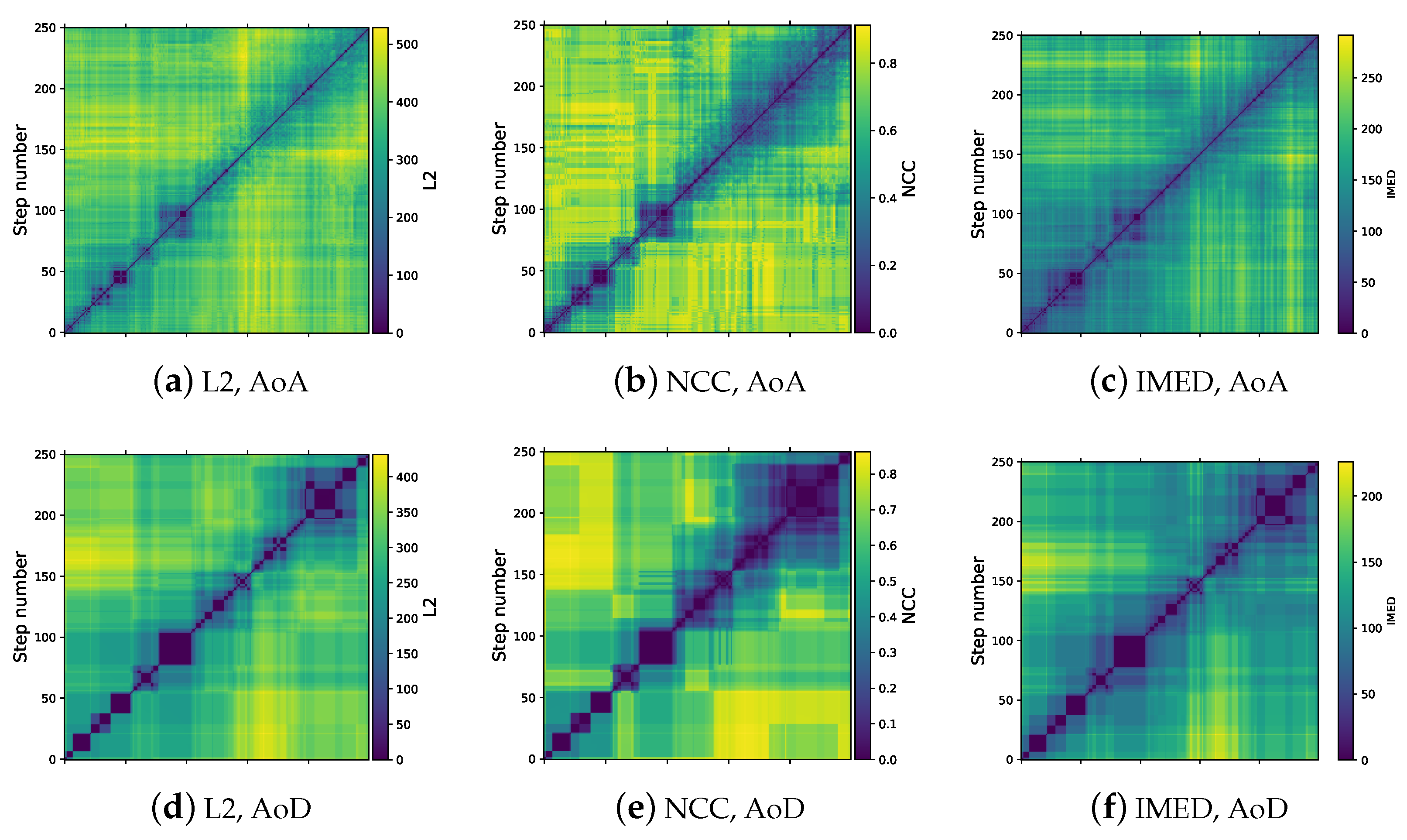
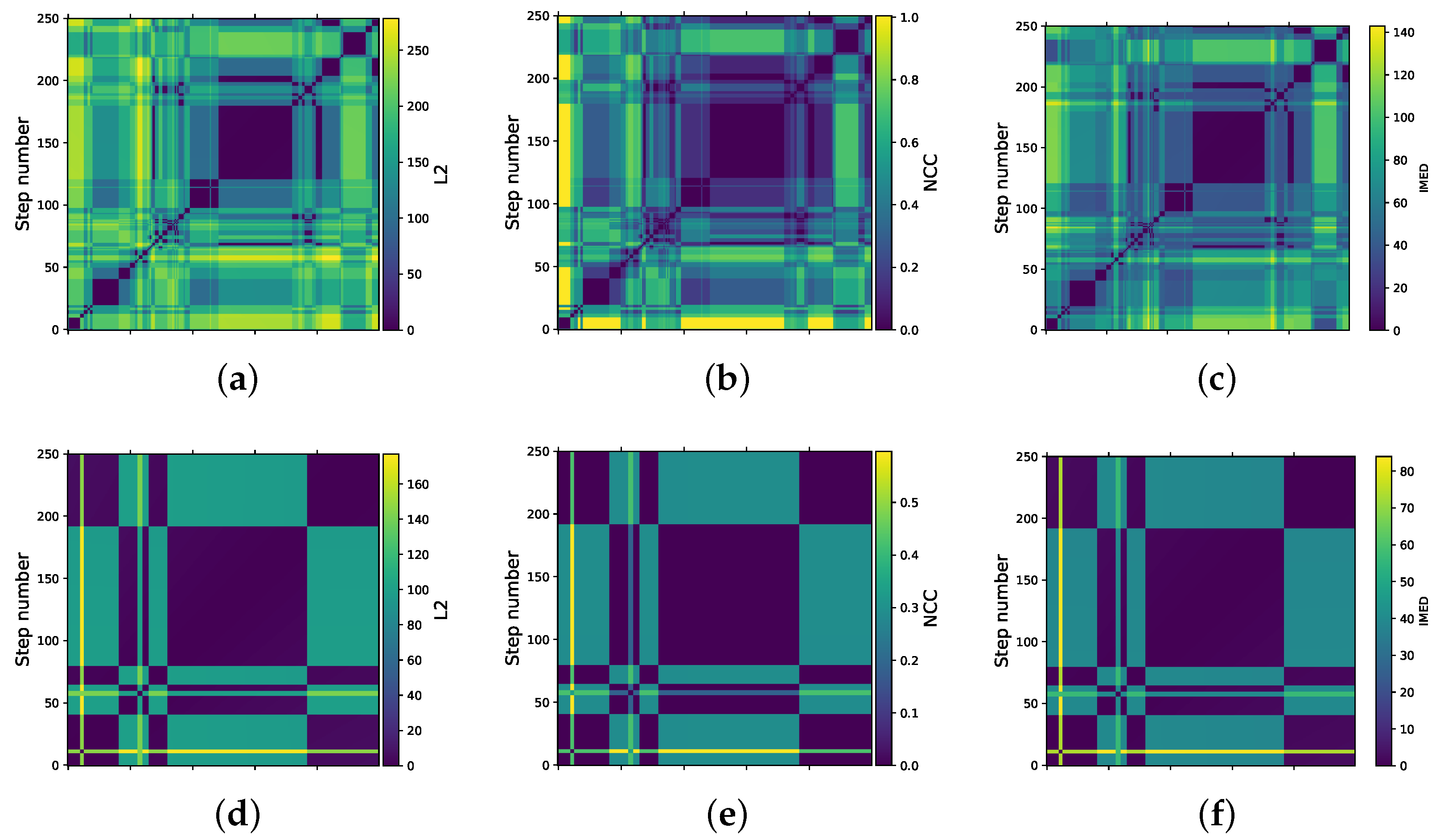
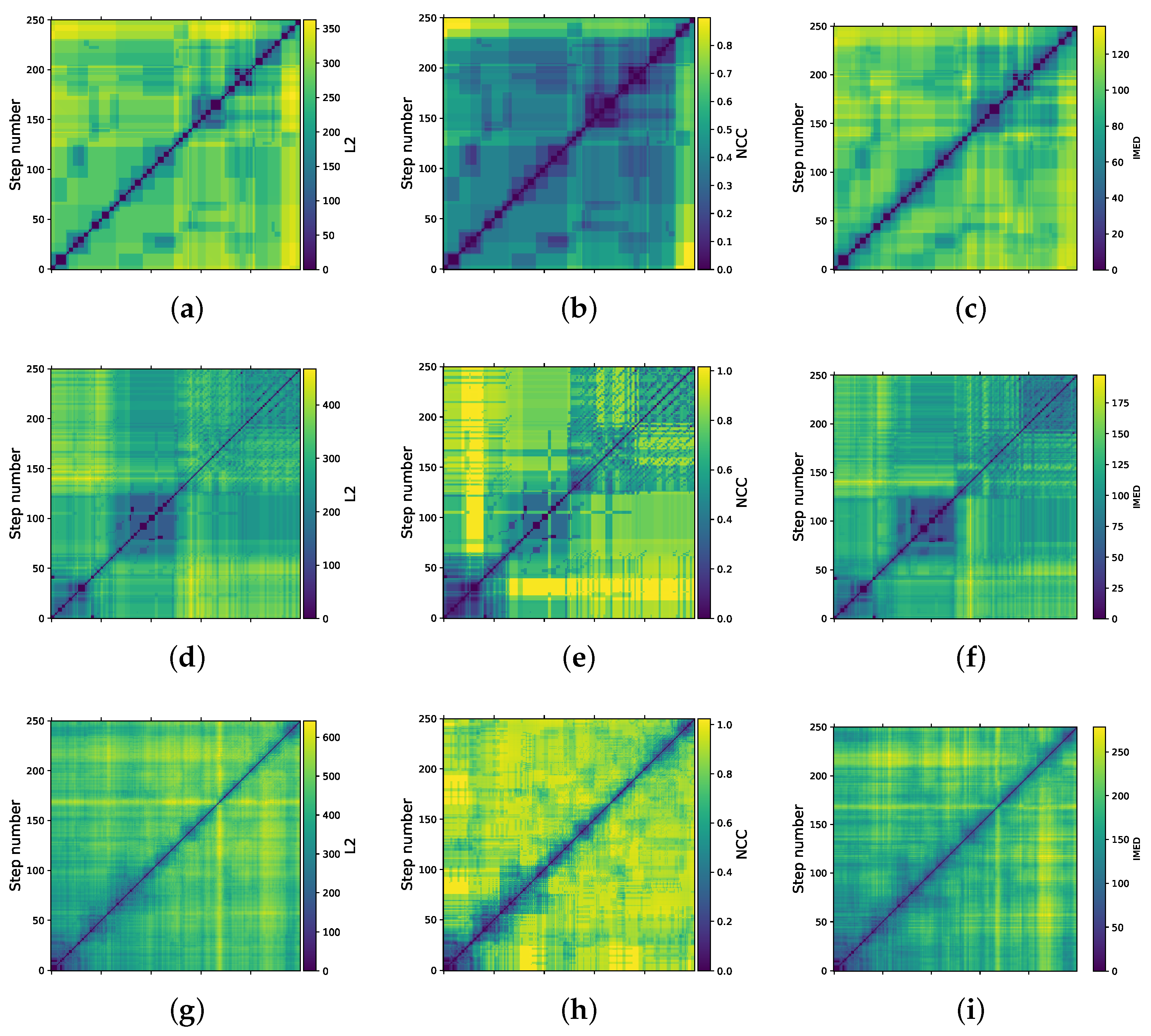
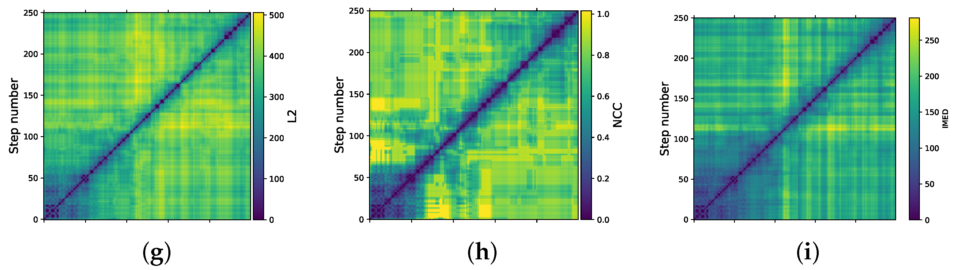
Figure 3, Figure 4, Figure 5 and Figure 6 show distance or dissimilarity matrices for the studied scenarios. Here, distances are computed using the previous measures pairwise between all steps of a trajectory. The diagonal elements are zero as they represent the distance between a frame and itself. By analyzing the presented data, we can observe that AoA yields a substantially blurrier picture than AoD. This can be explained by the shift in the coordinates at Rx due to its movement and the corresponding shift of the reference point. As could be expected, the image-oriented distance measures better cope with such a shift compared to the L2 distance (cf., e.g., Figure 3a,d vs. Figure 3b,e, or Figure 5a and Figure 6a vs. Figure 5b and Figure 6b). It can be deduced that for channel state prediction in the context of AoA, more specific loss functions could be worth considering instead of the MSE closely related to the L2 distance.

Let us now look in more detail at Figure 3 and Figure 4. The plotted distance matrices confirm that the SceLoS scenario is characterized by considerably more pronounced dynamics compared to SceNLoS, as can be seen from Figure 1. The sharp diagonal blocks in Figure 3d–f can be explained by beam clustering: it takes several trajectory steps for the strongest direct beam, in particular, to shift from one cluster to another, and this number grows as the angular distance between consecutive trajectory points diminishes. We also see that the distance matrices of both trajectories are characterized by pronounced diagonal blocks indicating trajectory segments with very similar data. However, sharp boundaries between the blocks may indicate difficulties in prediction when transitioning from one segment to another.

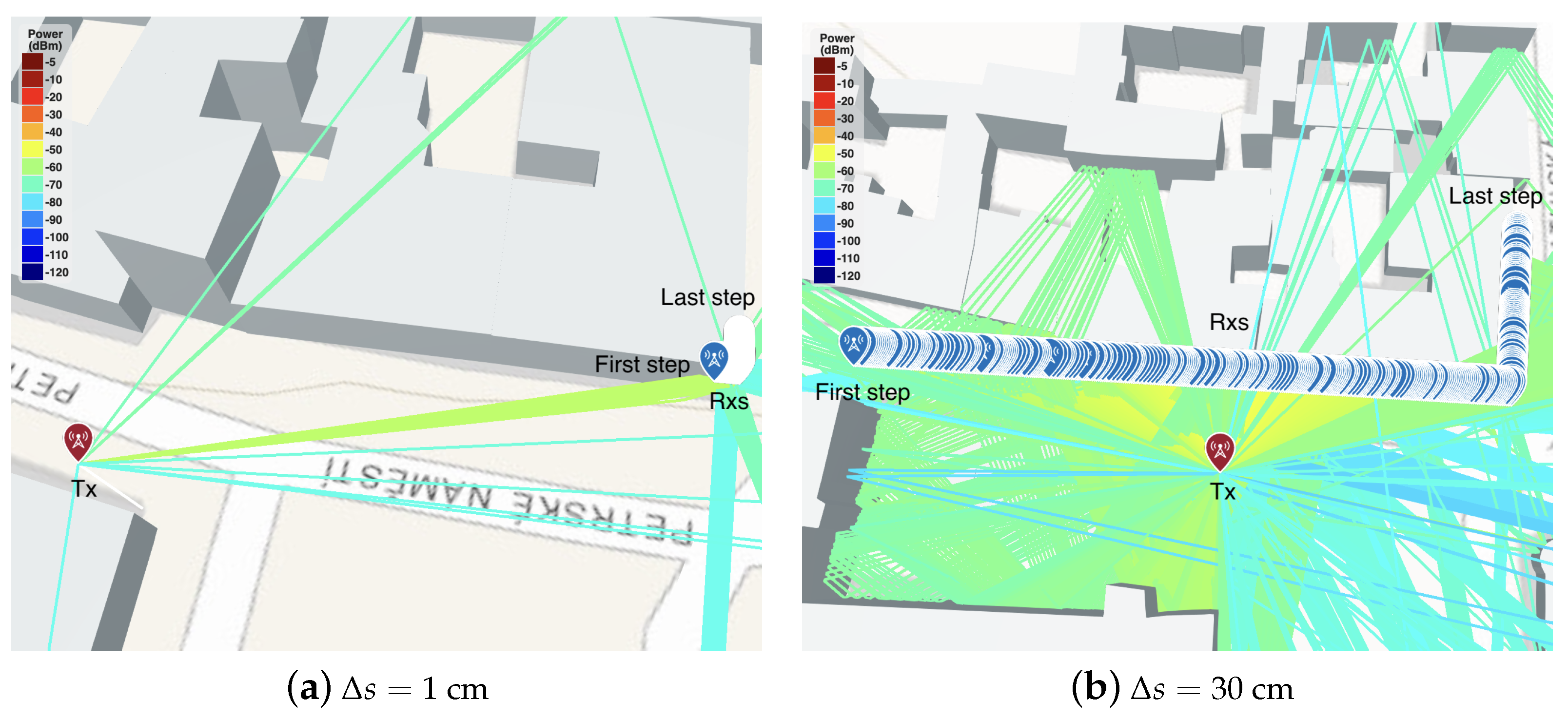
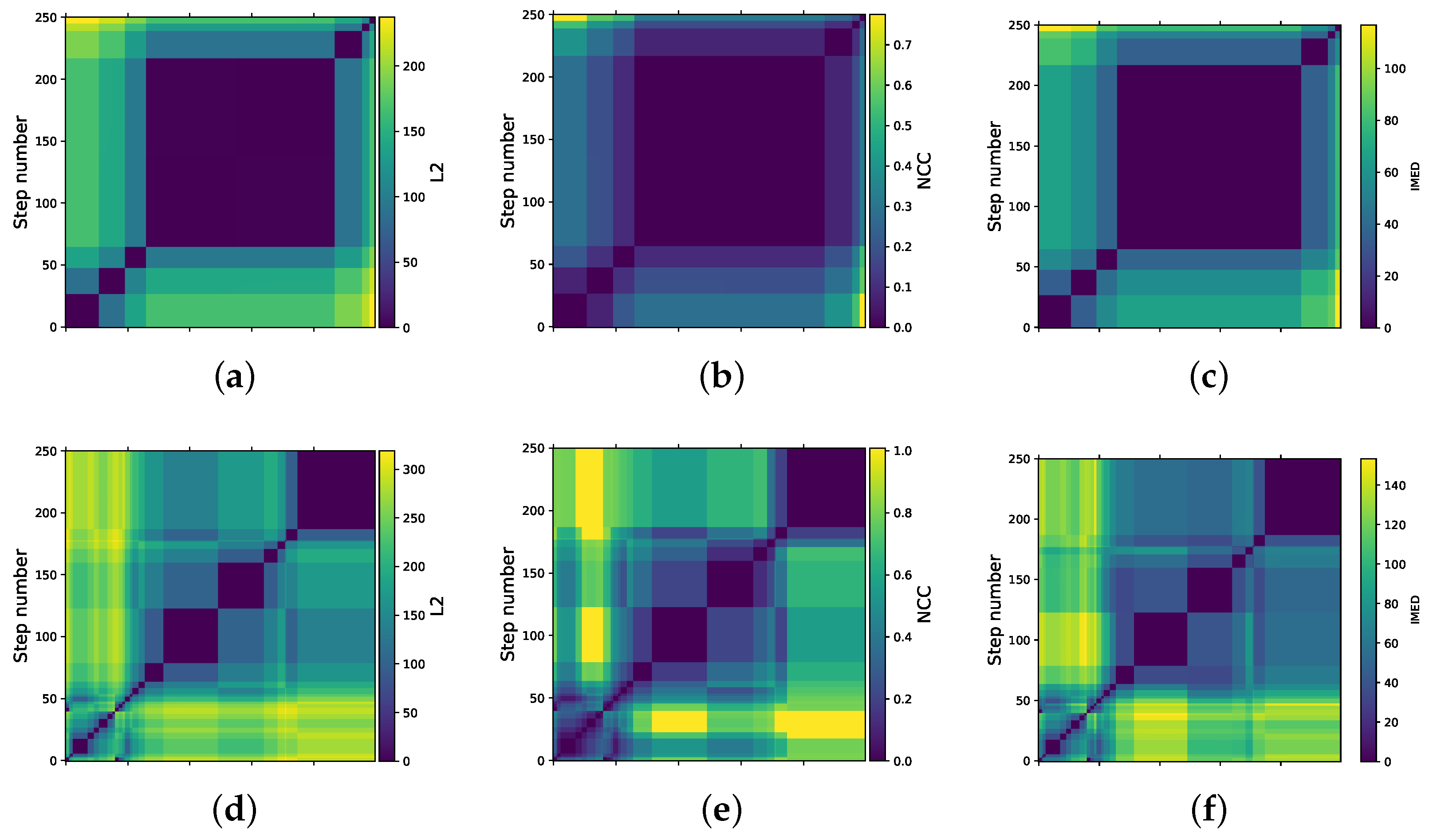
To obtain smoother transitions, two parameters can be adjusted: the frame resolution $K_{\theta }\times K_{\phi }$ and the step $\Delta s$. Therefore, for the SceTurn scenario, we consider three trajectories with $\Delta s$ set to 1, 10, and 30 cm. The trajectories are depicted in Figure 2 and the corresponding distance matrices in Figure 5 and Figure 6. It can be observed that by reducing the step $\Delta s$, not only do we obtain larger diagonal blocks, but also a smoother transition between them.

4. Channel State Prediction via ML Algorithms

Theoretically, the channel’s state characteristics may change over distances of a half wavelength. So, dynamic channel variations could lead to rapid changes in the channel’s state information, including AoA and AoD. However, as we have seen in Section 3, these changes happen at much wider scales. Identifying the scale, where the channel state prediction methods may still provide accurate approximations of AoA and AoD, are of critical importance for both beam-tracking algorithms and speeding up ray-tracing simulations.

Recently, deep neural networks (DNNs) have received considerable attention due to their decisive advantages: (i) DNNs can model complex non-linear relationships using multiple layers of an artificial neural network, and (ii) DNNs can achieve low complexity of mathematical operations. Thus, a DNN can be a suitable candidate for modeling the temporal behavior of mmWave channels.

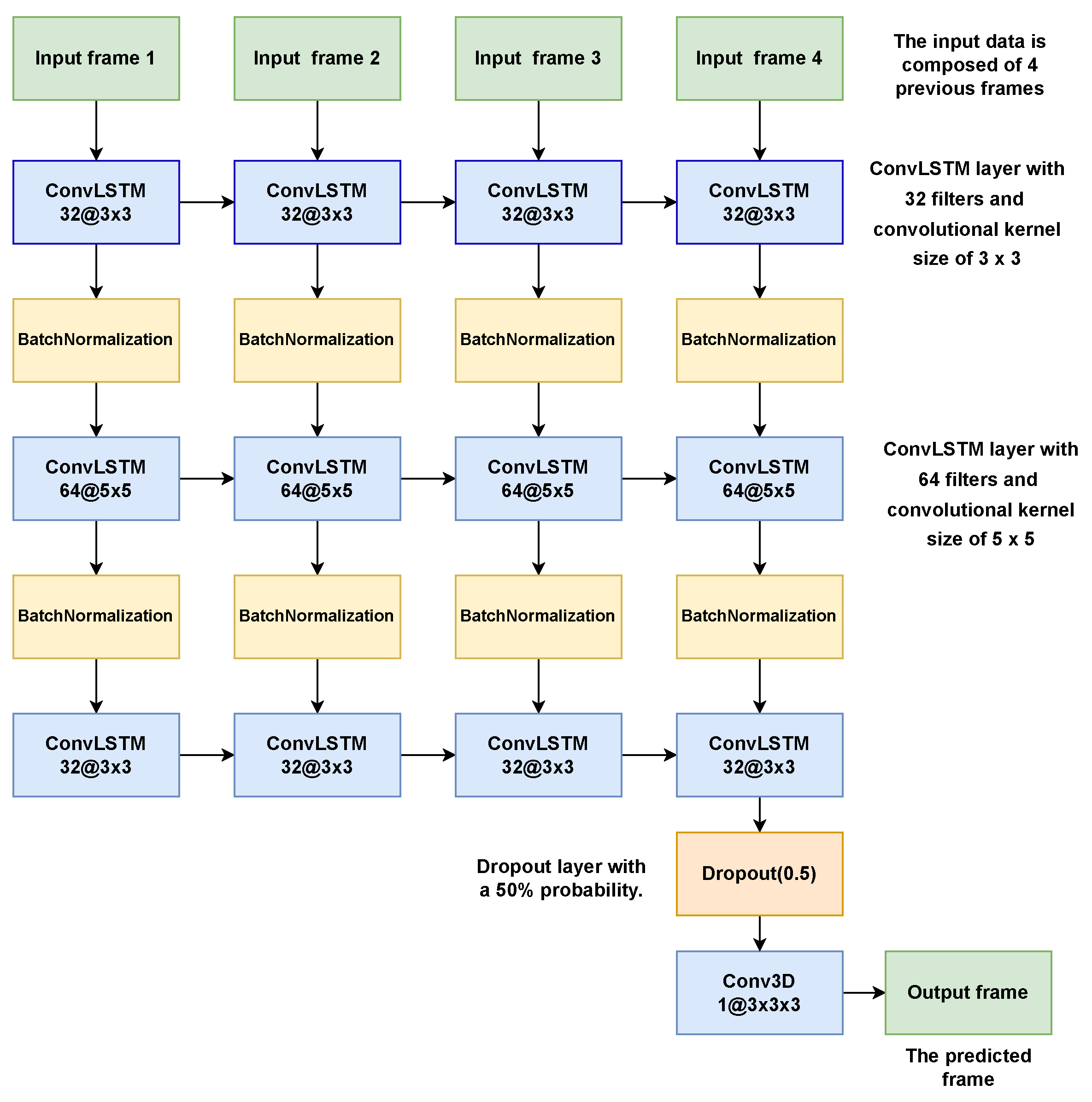
In this section, we propose a channel state prediction method that models rapidly-varying mmWave channels using DNNs. We employ a convolutional long short-term memory (ConvLSTM) architecture to predict the temporal evolution of $V_{\mathrm{X}}\left(s\right)$, based on N previous channel estimates $V_{\mathrm{X}}(s-N),\cdots ,V_{\mathrm{X}}(s-1)$.

4.1. Employed DNN Model

The channel state data representation introduced in Section 3 is characterized by spatial and temporal components. Convolutional neural networks have the ability to capture spatial features, while recurrent neural networks—and in particular, LSTM (long short-term memory)—can induce dependence over time. However, by simply stacking these kinds of layers, the dependence between space and time features may not be captured properly. In [37], a network structure able to capture spatio-temporal dependencies, ConvLSTM, is proposed. The ConvLSTM layer is a recurrent layer similar to LSTM, but internal matrix multiplications therein are exchanged with convolution operations. ConvLSTM can provide an effective tool for mmWave/THz channel estimations, as it has the ability to handle prediction from time series, where convolutional operations capture features while LSTMs capture time dependencies in the extracted features.

The proposed DNN model using ConvLSTM is shown in Figure 7. It is composed of nine layers. The input of the network is a three-dimensional tensor (N, $K_{\theta }$, $K_{\phi }$), where N represents the number of previous frames that the DNN uses to predict the next frames. We use $N=4$ in our setup. The second and third dimensions, $(K_{\theta },K_{\phi })$, represent the size of the input frame $V_{\mathrm{X}}$. The output of the network is a tensor of the size ($N_{\mathrm{out}}$, $K_{\theta }$, $K_{\phi }$), where $N_{\mathrm{out}}$ is the number of predicted frames, which in our case is one.

The first layer of the DNN is the input layer accepting $N=4$ frames of size $K_{\theta }\times K_{\phi }$. The second and sixth layers are ConvLSTM with 32 filters and a convolutional kernel of size $3\times 3$ to extract spatio-temporal features of the input data. The fourth is a convLSTM layer with 64 filters and a convolutional kernel of size $5\times 5$ to extract more detailed spatio-temporal feature information. The activation function of the convLSTM layers is of type tanh, which helps regulate the values passed through the network. After the second and fourth layers, there is a normalization layer that normalizes the output and provides better convergence. There is a dropout layer after the last normalization layer with a 50% probability in accordance with the recommended rates between 0.5 and 0.8 for hidden layers [38,39]. The dropout layer is added to enhance the robustness of the network and avoid overfitting. The output layer is Conv3D with a single filter and size $3\times 3\times 3$.

The previous model was implemented and trained in Python using the TensorFlow platform. We used the Adam algorithm and updated the network parameters with learning rate $0.001$ and mini-batch size of 50 samples for 50 epochs. MSE was used as the loss function.

4.2. Data Acquisition and Preprocessing

Ray tracing for data acquisition was performed with a 28 GHz carrier frequency, and the propagation environment was modeled to obtain propagation paths between Tx and Rx with the number of reflections up to 3. The data were collected from 10 different maps, and in each map, 10 different transmitter’s positions for 10 trajectories were modeled. Separate datasets were created for AoA and AoD and for various step size values, namely for $\Delta s=1,30,60,100$ cm. Each dataset ${\mathcal{D}}_{X,\Delta s}$, $X\in \{\mathrm{AoA},\mathrm{AoD}\}$, was then populated with sequences of size $S=5$ of consequent frames extracted from longer trajectories. Finally, the size of the datasets for each step size was set to 30,000 observations. Each dataset was split so that 70% was used for training the model and 30% for testing. We processed each dataset separately, so in what follows, indices X and $\Delta s$ are omitted when no confusion arises.

To improve prediction performance, we rescaled data in a dataset so that all entries lay in the range $[0,1]$ with 0 corresponding to empty clusters. More formally, let ${\left({\tilde{V}}^{\left(i\right)}\left(s\right)\right)}_{s=1,\cdots ,S}$ denote the original (before scaling) i-th data point of a dataset $\mathcal{D}$, $i=1,\cdots ,\left|\mathcal{D}\right|$, and let ${\tilde{v}}_{m,n}^{\left(i\right)}\left(s\right)$ denote the corresponding matrix entries, as previously. Then, after preprocessing, the dataset’s data points have the entries

$$v_{m,n}^{\left(i\right)}\left(s\right)=\frac{200-{\tilde{v}}_{m,n}^{\left(i\right)}\left(s\right)}{200-v_{min}\left(\mathcal{D}\right)}$$

(10)

for all $i=1,\cdots ,\left|\mathcal{D}\right|$, $s=1,\cdots ,S$, $m=1,\cdots ,K_{\theta }$, $n=1,\cdots ,K_{\phi }$, where

$$v_{min}\left(\mathcal{D}\right)=\underset{i,s,m,n}{min}{\tilde{v}}_{m,n}^{\left(i\right)}\left(s\right).$$

(11)

We also note that in each data point ${\left(V^{\left(i\right)}\left(s\right)\right)}_{s=1,\cdots ,S}$, frame $V^{\left(i\right)}\left(S\right)$ represents the label and frames ${\left(V^{\left(i\right)}\left(s\right)\right)}_{s=1,\cdots ,S-1}$ the features.

4.3. Metrics of Interest

As we described in Section 3.3, the row and column of a non-zero (or not equaling 200 before preprocessing) entry in an AoA/AoD frame $V\left(s\right)$ characterize the angles of the received/departed rays, and the value of the element corresponds to the path loss of the received ray. Thus, such a frame-like data representation makes our prediction task a combination of classification and regression problems, because we need to predict the positions of non-zero elements in the matrix and also their values.

Keras provides various metrics for evaluating regression and classification tasks [40]. To assess the performance of our proposed approach, we utilize the metrics Precision and Recall to quantify the accuracy of the coordinates and the mean squared error (MSE) to quantify the regression accuracy for the path loss value prediction. Let ${\widehat{V}}^{\left(i\right)}={\left({\widehat{v}}_{m,n}^{\left(i\right)}\right)}_{m=1,\cdots ,K_{\theta },n=1,\cdots ,K_{\phi }}$ denote the predicted value of $V^{\left(i\right)}\left(S\right)$. Denote by $\mathbf{1}\left\{A\right\}$ the indicator function such that $\mathbf{1}\left\{A\right\}=1$ if A is true and $\mathbf{1}\left\{A\right\}=0$ otherwise. Then, the numbers of true positive (TP), false positive (FP), and false negative (FN) results in the i-th data point can be computed, respectively, by

$$N_{\mathrm{TP}}^{\left(i\right)}=\sum _{m=1}^{K_{\theta }}\sum _{n=1}^{K_{\phi }}\mathbf{1}\{{\widehat{v}}_{m,n}^{\left(i\right)}>ϵ\}\mathbf{1}\{v_{m,n}^{\left(i\right)}\left(S\right)>ϵ\},$$

(12)

$$N_{\mathrm{FP}}^{\left(i\right)}=\sum _{m=1}^{K_{\theta }}\sum _{n=1}^{K_{\phi }}\mathbf{1}\{{\widehat{v}}_{m,n}^{\left(i\right)}>ϵ\}\mathbf{1}\{v_{m,n}^{\left(i\right)}\left(S\right)<ϵ\},$$

(13)

$$N_{\mathrm{FN}}^{\left(i\right)}=\sum _{m=1}^{K_{\theta }}\sum _{n=1}^{K_{\phi }}\mathbf{1}\{{\widehat{v}}_{m,n}^{\left(i\right)}<ϵ\}\mathbf{1}\{v_{m,n}^{\left(i\right)}\left(S\right)>ϵ\},$$

(14)

where $ϵ$ is a threshold between 0 and 1.

Now, the Precision metric (or the positive predictive value, PPV), which measures the percentage of correctly identified non-empty clusters among all clusters predicted as non-empty, can be computed, for a dataset $\mathcal{D}$, as

$$Precision\left(\mathcal{D}\right)=\frac{{\sum }_{i=1}^{\left|\mathcal{D}\right|}{N}_{\mathrm{TP}}^{\left(i\right)}}{{\sum }_{i=1}^{\left|\mathcal{D}\right|}{N}_{\mathrm{TP}}^{\left(i\right)}+{\sum }_{i=1}^{\left|\mathcal{D}\right|}{N}_{\mathrm{FP}}^{\left(i\right)}}.$$

(15)

Recall (or sensitivity), which measures the percentage of non-empty clusters that were identified, is given by

$$Recall\left(\mathcal{D}\right)=\frac{{\sum }_{i=1}^{\left|\mathcal{D}\right|}{N}_{\mathrm{TP}}^{\left(i\right)}}{{\sum }_{i=1}^{\left|\mathcal{D}\right|}{N}_{\mathrm{TP}}^{\left(i\right)}+{\sum }_{i=1}^{\left|\mathcal{D}\right|}{N}_{\mathrm{FN}}^{\left(i\right)}}.$$

(16)

We note that Precision and Recall are often interrelated, and improving Precision typically reduces Recall, and vice versa. Therefore, we tuned the threshold $ϵ$ of the two metrics to obtain the best value of prediction for both of them.

Finally, MSE is closely related to the L2 distance considered previously, and is given by

$$MSE\left(\mathcal{D}\right)=\frac{1}{\left|\mathcal{D}\right|K_{\theta }{K}_{\phi }}\sum _{i=1}^{\left|\mathcal{D}\right|}\sum _{n=1}^{K_{\theta }}\sum _{m=1}^{K_{\phi }}{({\widehat{v}}_{m,n}^{\left(i\right)}-v_{m,n}^{\left(i\right)}\left(S\right))}^2.$$

(17)

4.4. Numerical Results

In this section, we present model performance evaluation results from several experiments, in which we trained and tested the proposed DNN on the datasets ${\mathcal{D}}_{X,\Delta s}$ with $X\in \{\mathrm{AoA},\mathrm{AoD}\}$ and $\Delta s=1,30,60,100$ cm.

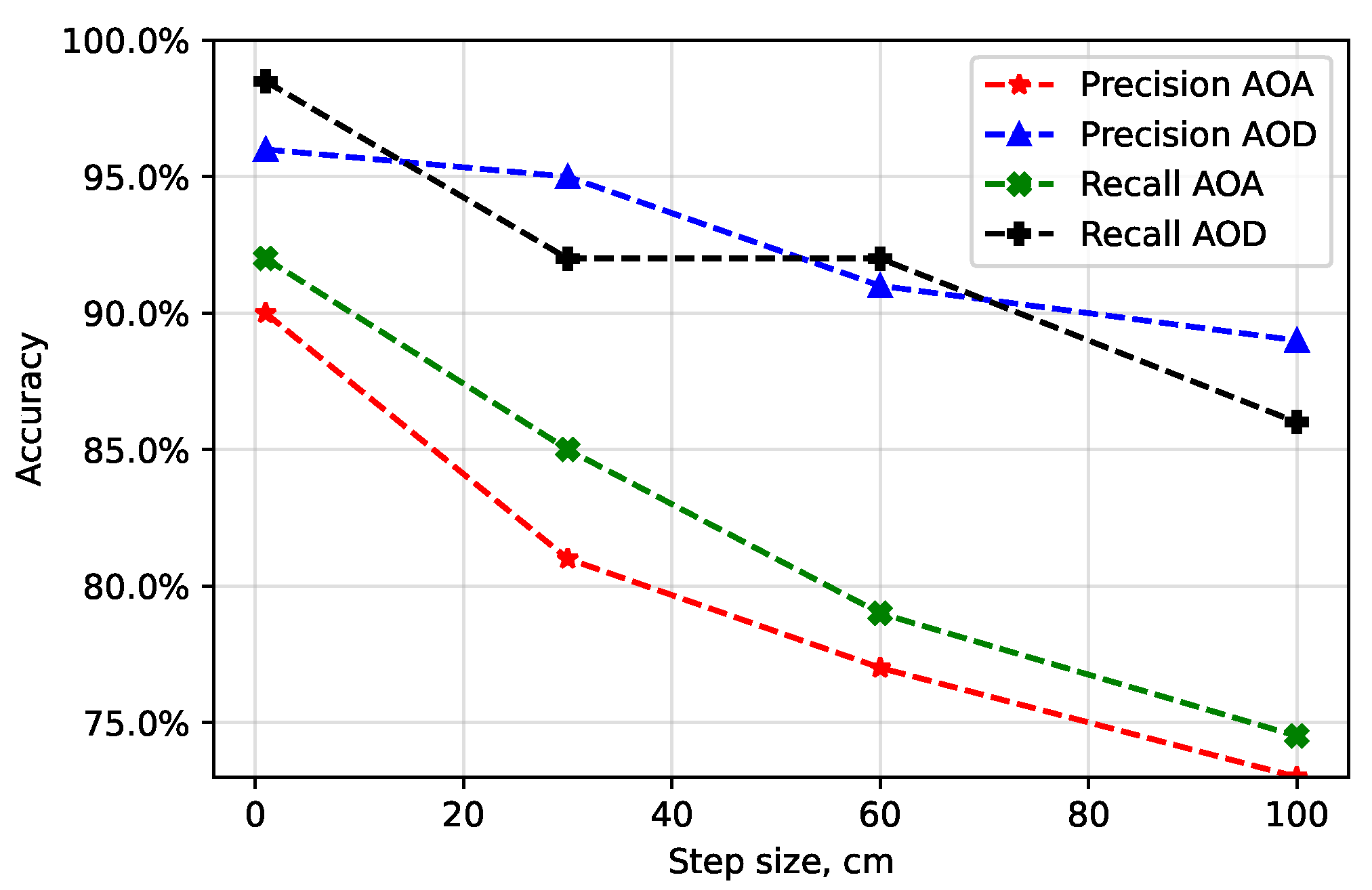
We start with Figure 8, presenting the achievable accuracy of predicting the coordinates of the elements in the frame via the considered metrics with respect to various values of the step size. As one may observe, the prediction probability of the AoD is better than the prediction probability of the AoA. The rationale is that, as we have seen in Section 3, the correlation between the consecutive frames is higher for the departing rays as compared to the incoming rays. Also, the proposed model can achieve approximately 97% prediction accuracy for the step size of 1 cm, and the achieved prediction decreases to 75% for the step size of 100 cm. This behavior is expected as the dependence between the consecutive frames decreases when the step size between two points on the trajectory increases.

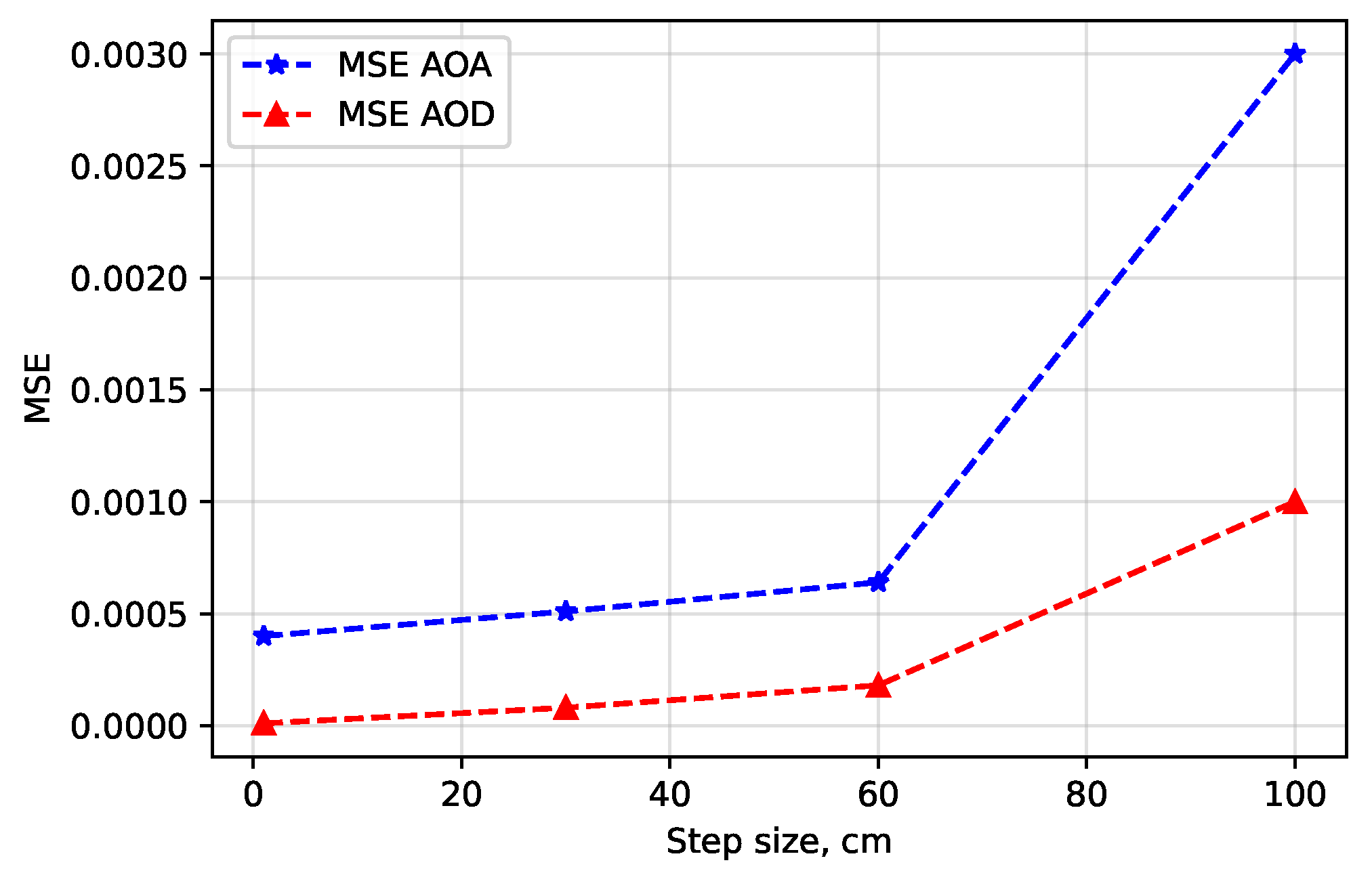
Further, in Figure 9, we present the observed MSE associated with predicting the path loss of the elements of the frame with respect to various values of the step size. The proposed model can achieve $5\times {10}^{-4}$ MSE for the step size of 1 cm. As one may observe, MSE remains almost intact up until the step size of 60 cm, and then it quickly increases to $5\times {10}^{-3}$ for the step size of 100 cm.

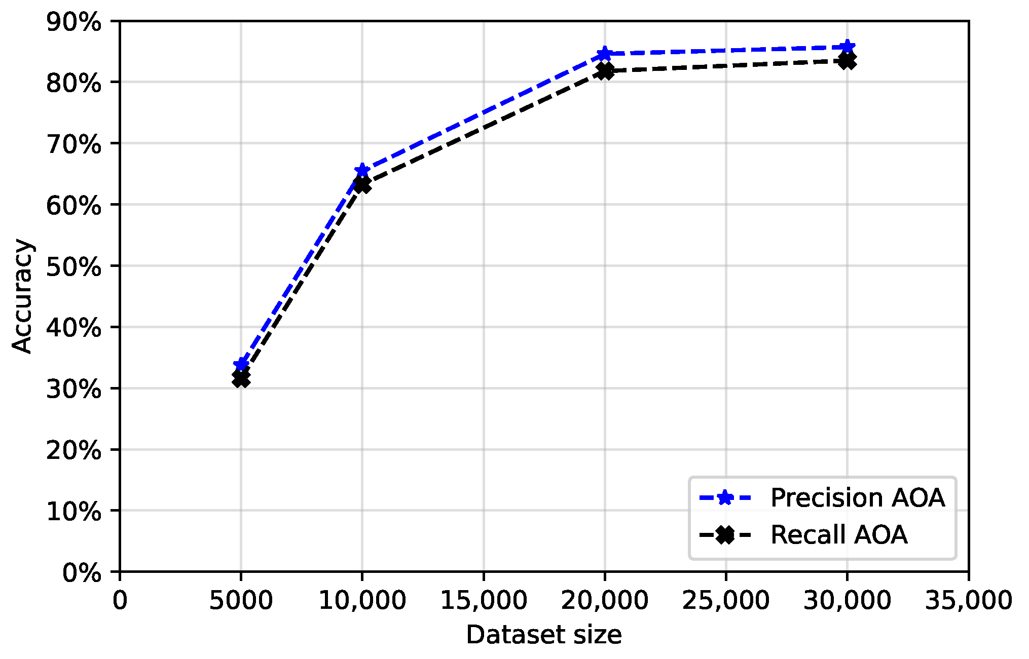
Figure 10 shows the model accuracy vs. the dataset size $\left|\mathcal{D}\right|$ obtained via 5-fold cross-validation. We observe that the model accuracy does not improve substantially after $\left|\mathcal{D}\right|$ = 20,000, which justifies our choice of the dataset size.

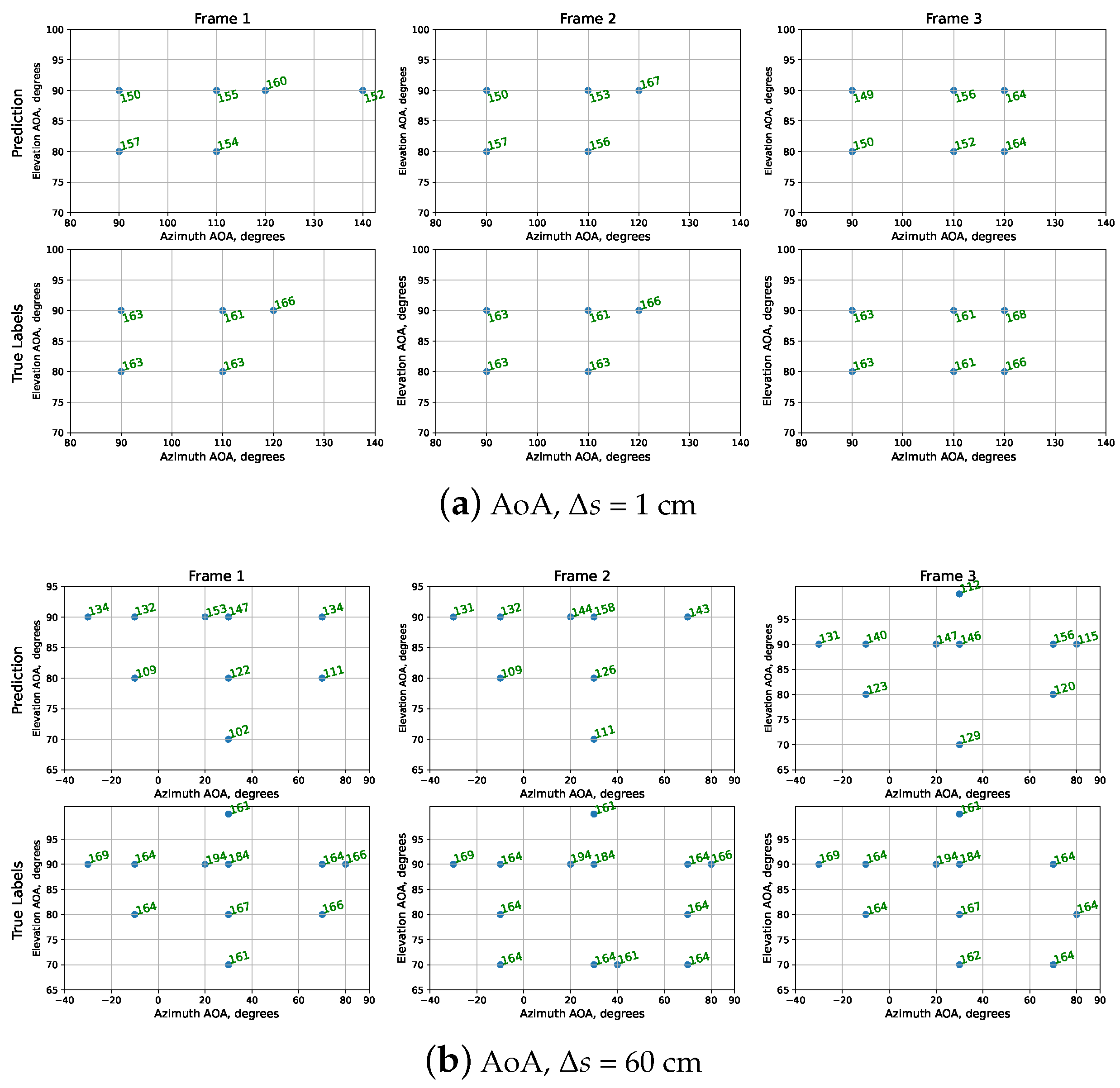
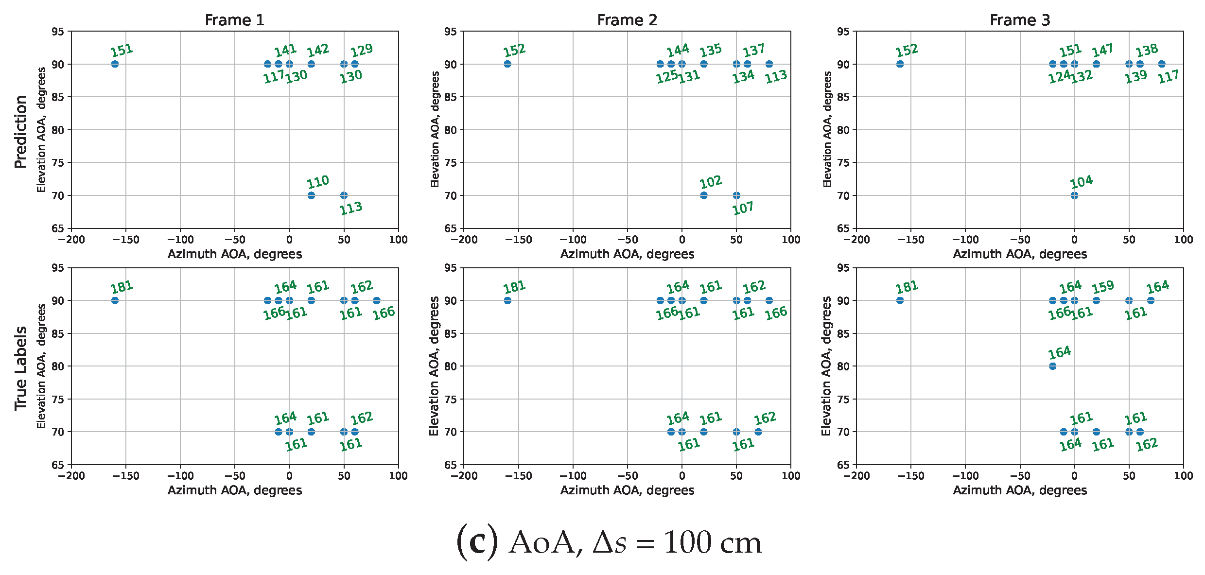
Finally, in Figure 11, we present some frame predictions. Here, three data points corresponding to consecutive Rx trajectory steps were chosen randomly from validation subsets of datasets ${\mathcal{D}}_{\mathrm{AoA},1}$, ${\mathcal{D}}_{\mathrm{AoA},60}$, and ${\mathcal{D}}_{\mathrm{AoA},100}$. Predicted frames are shown next to their ground-truth values, so as to illustrate the frame dynamics from step to step as well as the prediction efficiency. As one may observe, the difference between the true and predicted frames increases as the step size becomes larger. Specifically, for $\Delta s=1$ cm, the proposed algorithms predict the actual values almost perfectly for all the frame numbers, while for $\Delta s=100$ cm, there are occasional spikes in predicted data that become larger as the frame number increases.

5. Conclusions

In this paper, motivated the by the need for speeding up ray-tracing simulations and efficient beam tracking in future mmWave/THz systems, we first investigated the correlational properties of the channel state information in terms of AoD, AoA, and path loss in practical outdoor deployment scenarios. Then, we proposed a new data representation that makes it feasible to utilize a large set of powerful ML-based video frame interpolation and extrapolation techniques without substantial modification. Finally, we demonstrated how to predict channel state parameters and reported the prediction accuracy.

Our results show that the dependence in the AoA, AoD, and path loss is rather high, even at distances that are $k\approx 300$–600 times larger than the wavelength at 300 GHz. This implies that one may expect good interpolation and extrapolation results in ray tracing when the grid size is $k\lambda$, which drastically improves the simulation times. From the beam-tracking perspective, this implies that the beam-tracking interval can be as long as $t=k\lambda /v$, where v is the velocity of the UE. ML prediction results show that reliable prediction accuracy of AoA and AoD angles is feasible up to 60 cm distance with AoA being characterized by a higher MSE.

References

- Vannithamby, R.; Talwar, S. Towards 5G: Applications, Requirements and Candidate Technologies; John Wiley & Sons: Hoboken, NJ, USA, 2017. [Google Scholar]
- Polese, M.; Jornet, J.M.; Melodia, T.; Zorzi, M. Toward end-to-end, full-stack 6G terahertz networks. IEEE Commun. Mag. 2020, 58, 48–54. [Google Scholar] [CrossRef]
- Petrov, V.; Pyattaev, A.; Moltchanov, D.; Koucheryavy, Y. Terahertz band communications: Applications, research challenges, and standardization activities. In Proceedings of the 2016 8th International Congress on Ultra Modern Telecommunications and Control Systems and Workshops (ICUMT), Lisbon, Portugal, 18–20 October 2016; pp. 183–190. [Google Scholar]
- Balanis, C.A. Antenna Theory: Analysis and Design, 4th ed.; John Wiley & Sons: Hoboken, NJ, USA, 2016. [Google Scholar]
- Petrov, V.; Komarov, M.; Moltchanov, D.; Jornet, J.M.; Koucheryavy, Y. Interference and SINR in millimeter wave and terahertz communication systems with blocking and directional antennas. IEEE Trans. Wirel. Commun. 2017, 16, 1791–1808. [Google Scholar]
- Golos, E.; Daraseliya, A.; Sopin, E.; Begishev, V.; Gaidamaka, Y. Optimizing Service Areas in 6G mmWave/THz Systems with Dual Blockage and Micromobility. Mathematics 2023, 11, 870. [Google Scholar] [CrossRef]
- Dabiri, M.T.; Hasna, M. Pointing Error Modeling of mmWave to THz High-Directional Antenna Arrays. IEEE Wirel. Commun. Lett. 2022, 11, 2435–2439. [Google Scholar] [CrossRef]
- Moltchanov, D.; Sopin, E.; Begishev, V.; Samuylov, A.; Koucheryavy, Y.; Samouylov, K. A tutorial on mathematical modeling of 5G/6G millimeter wave and terahertz cellular systems. IEEE Commun. Surv. Tutor. 2022, 24, 1072–1116. [Google Scholar]
- Sopin, E.; Moltchanov, D.; Daraseliya, A.; Koucheryavy, Y.; Gaidamaka, Y. User association and multi-connectivity strategies in joint terahertz and millimeter wave 6G systems. IEEE Trans. Veh. Technol. 2022, 71, 12765–12781. [Google Scholar] [CrossRef]
- Giordani, M.; Polese, M.; Roy, A.; Castor, D.; Zorzi, M. A tutorial on beam management for 3GPP NR at mmWave frequencies. IEEE Commun. Surv. Tutor. 2018, 21, 173–196. [Google Scholar]
- Aguado-Agelet, F.; Formella, A.; Rabanos, J.; de Vicente, F.I.; Pérez-Fontán, F. Efficient ray-tracing acceleration techniques for radio propagation modeling. IEEE Trans. Veh. Technol. 2000, 49, 2089–2104. [Google Scholar] [CrossRef]
- Combeau, P.; Aveneau, L.; Vauzelle, R.; Pousset, Y. Efficient 2-D ray-tracing method for narrow and wideband characterization in micro-cellular configurations. IEE Proc.-Microw. Antennas Propag. 2007, 153, 502–509. [Google Scholar] [CrossRef]
- Alwajeeh, T.; Combeau, P.; Vauzelle, R.; Bounceur, A. A high-speed 2.5D ray-tracing propagation model for microcellular systems, application: Smart cities. In Proceedings of the 2017 11th European Conference on Antennas and Propagation (EUCAP), Paris, France, 19–24 March 2017; pp. 3515–3519. [Google Scholar] [CrossRef]
- Torres, R.P.; Valle, L.; Domingo, M.; Loredo, S. An efficient ray-tracing method for radiopropagation based on the modified BSP algorithm. In Proceedings of the Gateway to 21st Century Communications Village, VTC 1999-Fall, IEEE VTS 50th Vehicular Technology Conference (Cat. No.99CH36324), Amsterdam, The Netherlands, 19–22 September 1999; Volume 4, pp. 1967–1971. [Google Scholar]
- Hussain, S.; Brennan, C. Efficient Preprocessed Ray Tracing for 5G Mobile Transmitter Scenarios in Urban Microcellular Environments. IEEE Trans. Antennas Propag. 2019, 67, 3323–3333. [Google Scholar] [CrossRef]
- Yun, Z.; Iskander, M.; Zhang, Z. Fast ray tracing procedure using space division with uniform rectangular grid. Electron. Lett. 2000, 36, 895–897. [Google Scholar] [CrossRef]
- Kim, H.; Lee, H. Accelerated three dimensional ray tracing techniques using ray frustums for wireless propagation models. Prog. Electromagn. Res. 2009, 96, 21–36. [Google Scholar] [CrossRef]
- Degli-Esposti, V.; Fuschini, F.; Vitucci, E.M.; Falciasecca, G. Speed-Up Techniques for Ray Tracing Field Prediction Models. IEEE Trans. Antennas Propag. 2009, 57, 1469–1480. [Google Scholar] [CrossRef]
- Mataga, N.; Zentner, R.; Mucalo, A.K. Ray entity based postprocessing of ray-tracing data for continuous modeling of radio channel. Radio Sci. 2014, 49, 217–230. [Google Scholar] [CrossRef]
- Azpilicueta, L.; Rawat, M.; Rawat, K.; Ghannouchi, F.M.; Falcone, F. A Ray Launching-Neural Network Approach for Radio Wave Propagation Analysis in Complex Indoor Environments. IEEE Trans. Antennas Propag. 2014, 62, 2777–2786. [Google Scholar] [CrossRef]
- Wang, X.; Zhang, Z.; He, D.; Guan, K.; Liu, D.; Dou, J. A Multi-Task Learning Model for Super Resolution of Wireless Channel Characteristics. In Proceedings of the GLOBECOM 2022–2022 IEEE Global Communications Conference, Rio de Janeiro, Brazil, 4–8 December 2022; pp. 952–957. [Google Scholar] [CrossRef]
- Zhang, Z.; He, D.; Wang, X.; Guan, K.; Zhong, Z.; Dou, J. A Ray-tracing and Deep Learning Fusion Super-resolution Modeling Method for Wireless Mobile Channel. In Proceedings of the 2023 17th European Conference on Antennas and Propagation (EuCAP), Florence, Italy, 26–31 March 2023. [Google Scholar] [CrossRef]
- Wang, W.; Zhang, W. Signal processing for RIS-assisted millimeter-wave/terahertz communications. Natl. Sci. Rev. 2023, 10, nwad168. [Google Scholar] [CrossRef]
- Elbir, A.; Papazafeiropoulos, A. Hybrid Precoding for Multiuser Millimeter Wave Massive MIMO Systems: A Deep Learning Approach. IEEE Trans. Veh. Technol. 2019, 69, 552–563. [Google Scholar] [CrossRef]
- Guo, Y.; Wang, Z.; Li, M.; Liu, Q. Machine Learning Based mmWave Channel Tracking in Vehicular Scenario. In Proceedings of the 2019 IEEE International Conference on Communications Workshops (ICC Workshops), Shanghai, China, 20–24 May 2019; pp. 1–6. [Google Scholar] [CrossRef]
- Moon, S.; Kim, H.; Hwang, I. Deep learning-based channel estimation and tracking for millimeter-wave vehicular communications. J. Commun. Netw. 2020, 22, 177–184. [Google Scholar] [CrossRef]
- Ma, Y.; Ren, S.; Chen, W.; Quan, Z. Data-Driven Beam Tracking for Mobile Millimeter-Wave Communication Systems Without Channel Estimation. IEEE Wirel. Commun. Lett. 2021, 10, 2747–2751. [Google Scholar] [CrossRef]
- Panda, I.; Ramanath, S. Learning based Beam Tracking in 5G NR. In Proceedings of the 2020 International Conference on COMmunication Systems & NETworkS (COMSNETS), Bangalore, India, 7–11 January 2020; pp. 646–649. [Google Scholar] [CrossRef]
- Matlab. Available online: https://www.mathworks.com/ (accessed on 8 December 2022).
- OpenStreetMap. Available online: https://www.openstreetmap.org/ (accessed on 8 December 2022).
- Wireless Insite. Available online: https://www.remcom.com/ (accessed on 8 December 2022).
- Ansys HFSS. Available online: https://www.ansys.com/ (accessed on 8 December 2022).
- Winprop. Available online: https://web.altair.com/ (accessed on 8 December 2022).
- TR 38.901, Study on Channel Model for Frequencies from 0.5 to 100 GHz Technical Report Release V14.1.1. 2017. Available online: https://www.3gpp.org/ftp//Specs/archive/38_series/38.901/38901-e11.zip (accessed on 8 December 2022).
- Laplante, P.A. Encyclopedia of Image Processing, 1st ed.; CRC Press, Inc.: Boca Raton, FL, USA, 2018. [Google Scholar]
- Wang, L.; Zhang, Y.; Feng, J. On the Euclidean distance of images. IEEE Trans. Pattern Anal. Mach. Intell. 2005, 27, 1334–1339. [Google Scholar] [CrossRef]
- Shi, X.; Chen, Z.; Wang, H.; Yeung, D.Y.; Wong, W.K.; Woo, W.C. Convolutional LSTM Network: A Machine Learning Approach for Precipitation Nowcasting. Adv. Neural Inf. Process. Syst. 2015, 28, 1–11. [Google Scholar]
- Srivastava, N.; Hinton, G.; Krizhevsky, A.; Sutskever, I.; Salakhutdinov, R. Dropout: A Simple Way to Prevent Neural Networks from Overfitting. J. Mach. Learn. Res. 2014, 15, 1929–1958. [Google Scholar]
- Madaeni, F.; Chokmani, K.; Lhissou, R.; Homayouni, S.; Gauthier, Y.; Tolszczuk-Leclerc, S. Convolutional neural network and long short-term memory models for ice-jam predictions. Cryosphere 2022, 16, 1447–1468. [Google Scholar] [CrossRef]
- Keras. Available online: https://keras.io/api/metrics/ (accessed on 4 August 2023).