An Effective Partitional Crisp Clustering Method Using Gradient Descent Approach

Abstract

Enhancing the effectiveness of clustering methods has always been of great interest. Therefore, inspired by the success story of the gradient descent approach in supervised learning in the current research, we proposed an effective clustering method using the gradient descent approach. As a supplementary device for further improvements, we implemented our proposed method using an automatic differentiation library to facilitate the users in applying any differentiable distance functions. We empirically validated and compared the performance of our proposed method with four popular and effective clustering methods from the literature on 11 real-world and 720 synthetic datasets. Our experiments proved that our proposed method is valid, and in the majority of the cases, it is more effective than the competitors.

1. Introduction: Background and Motivation

Clustering is a method of partitioning a set of data points into partitions such that the within-partition data points are as homogeneous as possible and the between-partitions data points are as heterogeneous as possible. The partitions are referred to as clusters. Clustering is a crucial tool in data science, knowledge discovery and artificial intelligence and has various applications in disciplines such as biology, social science, neuroscience, computer science, etc. Thus, not surprisingly, an enormous number of papers have been published addressing different aspects of clustering.

Recently, a comprehensive survey on this subject has been published [1] that extends the well-accepted taxonomy of clustering methods and reviews the trends and open challenges. The authors classified the clustering methods into (i) hierarchical and (ii) partitional clusterings. Furthermore, they categorized the hierarchical clusterings into (i-a) agglomerative and (i-b) divisive clusterings: and they categorized the partitional clusterings into (ii-a) crisp, (ii-b) mixture resolving and (iii-c) fuzzy clusterings. Figure 1 depicts the three first levels of this taxonomy.

Furthermore, the authors of this survey considered the recent research works devoted to adaptations of clustering methods to various disciplines as the recent trends in this area of research. Moreover, they listed nine open issues in clustering algorithms, and the “effectiveness” of clustering methods is one of them.

Our line of thought aligned with this survey. Therefore, the main objective of the current research was to propose an effective clustering method to improve the clusters recovery results. Therefore, inspired by the success story of the gradient descent algorithm in the supervised learning tasks [2], we proposed a generic clustering objective function and then adopted the gradient descent approach to optimize it. As a by-product of our proposed method and to increase its flexibility, we implemented it using an automatic differentiation library called JaX [3]. With this setting, any differentiable distance function can be applied, and this can be considered as an additional tool for further improvements of the clusters recovery results.

It is noteworthy to add that the current research introduces the following contributions:

• Proposing a generic clustering criterion with the possibility of utilizing any differentiable distance functions in it;
• Adapting the gradient descent approach for the task of partitional crisps clustering;
• Equipping the proposed method to automatic differentiation as a by-product for further improvements of cluster recovery results.

We empirically validated and compared the performance of our proposed method with four popular and effective clustering methods on real-world and synthetic datasets. Our experiments proved that in most cases, our proposed method enhances the cluster recovery results. More so, our flexible implementation serves as a supplementary device for further clustering results’ improvements.

The rest of the paper is organized as follows. Section 2 reviews the previous work. Section 3 describes our proposed clustering. Section 4 explains the experimental setting for scrutinizing the hyperparameters of our proposed method and comparing it with four effective clustering methods from the literature. It presents (a) competitors; (b) datasets, both real-world and artificially generated; (c) criteria for assessment of the quality of experiments; and (d) the pre-processing technique. The study of the proposed methods’ hyperparameters is reported in Section 5. Section 6 describes the results of our experiments. Finally, Section 7 concludes the paper and presents our future directions.

2. Previous Work

This section concisely reviews the principles of the clustering algorithms with respect to the taxonomy mentioned earlier. However, since the gradient descent clustering is not covered in [1] and it is the cornerstone of the current research, Section 2.3 reviews the scarce number of previously published gradient descent (GD) clustering papers.

2.1. Partitional Clusterings

The partitional clusterings assign data points into K clusters by optimizing some clustering criteria. This class of clustering methods can be further classified into three subclasses: (i) crisp/hard, (ii) fuzzy, and (iii) mixture-resolving clusterings. In the first subclass, each data point belongs only to one cluster, while on the contrary, in the fuzzy clustering methods, each data point can belong to more than one cluster. The third subclass, mixture resolving, assumes a world model leading to a probabilistic distribution for which its parameters should be inferred from the data. The rest of this subsection is devoted to reviewing these three subclasses.

Presumably, K-means [4] can be considered the most well-known instance of the first subclass. K-means minimizes the total squared errors of within-cluster. K-medoids [5,6] minimizes the dissimilarities of within-cluster data points while selecting some of the data points as centroids, referred to as medoids, instead of the average data points of the clusters. The density-based clusterings [7] recover the clusters by separating the dense regions from low-density regions in the feature space. For instance, the density-based spatial clustering of applications with noise [8], DBSCAN, finds core samples of high-density regions and expands clusters from them. Ordering points to identify the clustering structure [9,10], OPTICS, tackles the issue of finding the proper range parameter in DBSCAN.

Recently, a new set of (meta)heuristic clustering methods has emerged [11,12,13,14,15]. The main objective of this set of methods is to spontaneously recover the cluster structures and the number of clusters without prior information. These methods are mainly nature-inspired and contain an immense number of hyperparameters, which in our opinion contradicts the ultimate goal of clustering. It ought to mention that the results in [14,15] did not enhance the traditional methods’ cluster recovery results. These methods can be categorized under the search-based clusterings [1] umbrella.

The deep clustering methods are another set of newly emerged methods. These methods use deep neural networks [16,17], DNNs, to learn a cluster-friendly representation of data followed by a traditional clustering algorithm to recover clusters from the obtained data representation by DNN. Various DNN algorithms have been applied to learn the cluster-friendlier data representation; Ref. [18] provided a systematic overview of this subject.

Contrary to crisp clusterings in fuzzy clusterings, the clusters overlap with a degree of membership based on fuzzy logic [19]. The initial fuzzy clusterings had problems with outliers, noise and initial partition dependencies [20]. The algorithms proposed in [21,22] tried to tackle those issues. Ref. [23] combined fuzzy C-means with mini-batch gradient descent with regularization. The authors in [24] proposed a unified combination of K-means and C-means methods. The authors in [25] proposed a novel technique to find the optimal number of clusters.

The underlying assumption of mixture-resolving clusterings is that the observed data points are generated from a mixture of probabilistic distributions whose parameters should be inferred from the dataset. These methods are model-based, and a statistical model or a priori should be known ahead of clustering. The expectation-maximization algorithm is the cornerstone of this category of methods [26,27].

2.2. Hierarchical Clusterings

This category of clusterings methods groups the data points to construct a hierarchical structure: the grouping procedure can be performed either in a bottom–up (agglomerative) or a top–down (divisive) fashion [20]. The agglomerative methods [28,29] initially start by assigning each data point to a singleton cluster and then iteratively merge every two clusters until (i) all clusters are merged into the root node or (ii) some stopping criteria are met. The root node represents the entire dataset. The divisive hierarchical methods start from a single cluster, representing the data, then in a top–down fashion splitting the clusters.

The merging or splitting decision generalizes the distance metrics of individual data points to distance metrics of subsets of data points. The distance metrics between subsets usually is referred to as linkage metrics. The single linkage—when the least interconnecting (dis)similarity between two components is considered [30], complete linkage, average linkage, McQuitty methods [31], median and centroid methods [32] are some of the prominent agglomerative (bottom–up) clustering methods employing different linkage metrics. Ward’s methods [33] are another type of agglomerative clustering in which instead of linkage metrics, the merging decision is based on the optimal values of an objective function [34]. Balanced iterative reducing and clustering using hierarchies [35], BIRCH, is an online and memory-efficient agglomerative algorithm developed for large-scale datasets. The clustering using representative (CURE) addresses the drawbacks of BIRCH and is more robust to outliers, and it claims to detect different clusters’ shapes and sizes.

The divisive methods are the reverse of agglomerative clustering. They start by splitting the entire dataset into smaller subsets until the predefined number of clusters is detected [36,37,38]. The natural splitting solution would be to analyze all possible bipartitions and select the two optimal ones. This solution is computationally expensive, and various divisive approaches have been developed to tackle this. For instance, bisecting K-means [39], reference point-based dissimilarity measure [40], and particle optimizer [41] are some of the efforts proposed to tackle this expensive computational complexity. In principle, divisive methods can be classified into monothetic and polythetic classes. The former uses the features one-by-one and was initially proposed for binary data [42,43] but later applied to multi-modal data. The latter class uses all features at once and utilizes the distance values [44,45].

2.3. Gradient Descent Clusterings

The majority of the previous GD-based clustering papers used it to optimize the proposed clustering objective function. For instance, the authors in [46] proposed a new graph cut clustering. They derived the graph cut using the Parzen windowing; then, they used GD for optimizing the proposed graph cut. In [47], it was employed to optimize the Gaussian kernel density estimators; similarly, ref. [48] used this optimization algorithm to learn Gaussian mixture models parameters. The methods proposed in [49,50] exploited GD to improve the K-means clustering performance; and the authors in [51] applied it for fuzzy clustering. While the previous works were devoted to partitional clustering, the authors in [52] adopted gradient descent for hierarchical clustering by embedding the representation of tree structures in hyperbolic space.

On the contrary, there are few papers in which they used GD for cluster refinement purposes or fine-tuning the parameters of the proposed methods. For instance, in [53], a fuzzy clustering method was proposed, and GD was used to fine-tune the parameters of the constructed fuzzy model to obtain a more accurate fuzzy model from the given input–output data. The authors in [54] used fuzzy clustering methods to construct the similarity matrices of each partition. Next, they aggregated partitions employing the direct sum of weighted vectors. Finally, the ultimate membership matrix was calculated by optimizing the sum of square errors through the gradient descent method.

3. Methodology

3.1. Problem Formulation, Notation and Motivation of the Proposed Method

Consider a set of N data points $X={\left\{{\mathbf{x}}_i\right\}}_{i=1}^N$ for ${\mathbf{x}}_i\in {\mathbb{R}}^V$, where V is the dimensionality of the data points. Our goal is to partition X into K subsets, $S={\left\{s_k\right\}}_{k=1}^K$, such that (i) the within-cluster data points are as homogeneous as possible and (ii) the between-clusters data points are as heterogeneous as possible. To accomplish our goal, as a standard practice, we associate each subset with the so-called cluster centroid ${\mathbf{c}}_k$ forming our set of centroids C. Then, we define the following clustering criterion:

$$F(X,S,C)=\sum _{k=1}^K\sum _{i=1}^{N}f({\mathbf{x}}_i,{\mathbf{c}}_k)$$

(1)

where $f:X\times C⟶\mathbb{R}$ represents a (generic) distance function that will be applied to measure the distance between the data point ${\mathbf{x}}_i$ and the centroid ${\mathbf{c}}_k$.

In principle, optimizing clustering criterion (1) in a reasonable time depends on (i) the availability of any prior knowledge, including the number of clusters, (ii) the expected cluster membership type, i.e., being crisp or fuzzy, and (iii) the choice of the distance function, i.e., being differentiable or not. For instance, by defining f to be the Euclidean distance and pursuing the alternating optimization algorithm, for a given number of clusters, the popular K-means method [4] can be obtained. In contrast, using the same distance function in the one-by-one cluster extracting strategy [55], when the number of clusters is not known, leads to the i-K-means method [56]—it extended to a more complex data structure in [57] recently. Interested readers may advise [20,56] for more details on clustering methods and [58] about generic optimization algorithms.

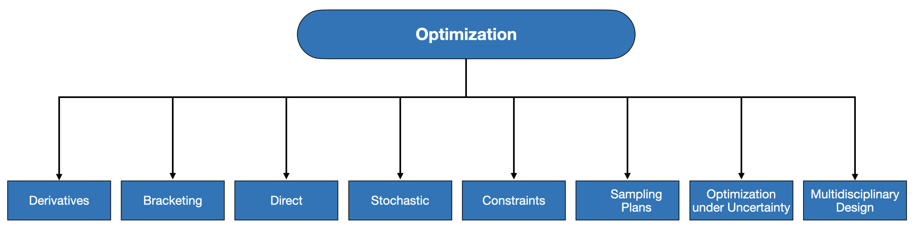
The authors in [58], a recent and comprehensive textbook on optimization algorithms, categorized the existing algorithms into eight families of methods, as shown in Figure 2. They explained the conditions for which each family is applicable and discussed the challenges and limits of the algorithms under consideration. Among those possible options, due to the simplicity, intuitiveness, and yet proven effectiveness of the derivative-based methods, we were interested in applying them. This family can be further categorized into first-order and second-order methods, for which, in the multivariate optimization setting, the former relies on gradients, and the latter relies on Hessian information to direct the search to find an optimum.

Although the second-order methods are proven to be more effective than first-order methods, as we observed in our preliminary experiments, they suffer from expensive computational complexity. Therefore, despite some of the disadvantages of the first-order methods such as their sensitivity to seed initialization or the step size, the possibility of being stuck in local minima or close to the global minimum, etc., we decided to proceed with first-order methods. This set of methods starts from a random initial point, and based on the fact that the negative of the gradient represents the steepest descent, iteratively modifies the initial guess to find a minimum using the gradient information.

In this work, we assumed that the clusters are crisp, and their number, K, is given. Moreover, although any differentiable distance function can be exploited, we limit our choice to the Minkowski distance with p-values limited to $1\le p\le 4$. This setting enables us to adopt the celebrated gradient descent optimization algorithm, a well-known and popular member of first-order-derivative-based optimization methods, for the task of cluster recovery. Since gradient descent is an iterative method, we should update our notation by adding subscript $\left(t\right)$ to reflect the concept of iterations. Concretely, we denote the set of cluster centroids at iteration t with $C^{\left(t\right)}={\left\{{\mathbf{c}}_k^{\left(t\right)}\right\}}_{k=1}^K$. Similarly, we denote the set of detected clusters at iteration t with $S^{\left(t\right)}={\left\{s_k^{\left(t\right)}\right\}}_{k=1}^K$.

3.2. Gradient Descent Clustering Methods

Our proposed gradient descent clustering (GDC) method consists of three constituents: (A) cluster assignment criterion, (B) cluster update rules and (C) convergence condition. In the remainder of this subsection, we explain them.

The first constituent of GDC, the cluster assignment criterion, is shown in Equation (2):

$$\underset{k}{argmin}f({\mathbf{x}}_i,{\mathbf{c}}_k^{\left(t\right)})<f({\mathbf{x}}_i,{\mathbf{c}}_j^{\left(t\right)}),\forall j\ne k.$$

(2)

that is, at iteration t, the data point ${\mathbf{x}}_i$ will be assigned to the cluster k for which its distance to the centroid ${\mathbf{c}}_k^{\left(t\right)}$, is minimum.

The second constituent of GDC, i.e., the update rule, in its Vanilla form is explained in Equation (3):

$${\mathbf{c}}_k^{(t+1)}={\mathbf{c}}_k^{\left(t\right)}-\alpha {\nabla }_{{\mathbf{c}}_k^{\left(t\right)}}f({\mathbf{x}}_i,{\mathbf{c}}_k^{\left(t\right)}),$$

(3)

where $\alpha$ represents the so-called step size, and $\nabla c_k^{\left(t\right)}$ is the gradient of the distance function, f, with respect to the k-th centroid at iteration t evaluated with the data point ${\mathbf{x}}_i$. It ought to point out that our preliminary experiments, aligned with the results of [59], showed that the per-data-point, or online, update rule is significantly more efficient than the batch version of the gradient descent algorithm; therefore, we always update the centroids in an online manner.

Furthermore, our unreported experiments were aligned with the well-known fact that the Vanilla update rule, i.e.,  Equation (3), is prone to slow convergence, especially at nearly flat surfaces [58]. To tackle this issue, accumulating momentum was proposed [60]. However, this accumulation may lead to overshoots at the valley floor; to avoid the overshooting, we exploit the Nesterov-accelerated momentum [61] to modify the gradient at the projected future position as follows:

$$\begin{array}{c}\hfill \begin{array}{c}\hfill {\mathbf{v}}^{(t+1)}={\beta }_1{\mathbf{v}}^{\left(t\right)}-\alpha {\nabla }_{{\mathbf{c}}_k^{\left(t\right)}}f({\mathbf{x}}_i+{\beta }_1{\mathbf{v}}^{\left(t\right)},{\mathbf{c}}_k^{\left(t\right)})\end{array}\end{array}$$

(4a)

$$\begin{array}{c}\hfill \begin{array}{c}\hfill {\mathbf{c}}_k^{(t+1)}={\mathbf{c}}_k^{\left(t\right)}+{\mathbf{v}}^{(t+1)}\end{array}\end{array}$$

(4b)

where ${\mathbf{v}}^{\left(t\right)}$ is the so-called momentum vector, with initial values of zero, and is the accumulation of the gradient’s history up to iteration t. The coefficient ${\beta }_1\in [0,1)$ is a hyperparameter that decays the momentum. We empirically study its impact and show that any value $\in [0.3,0.6]$ leads to superior results. It is noteworthy to add that since at each iteration, we compute the gradients of f with respect to the closet centroid of ${\mathbf{x}}_i$, thus, adding ${\mathbf{v}}^{\left(t\right)}$ to ${\mathbf{x}}_i$ usually has a desirable impact. More precisely, consider the ideal situation for which the data and the momentum vectors point to the same direction in the (feature) space. Thus, this addition decreases the gradients, which is desirable to avoid overshooting. Meanwhile, the first term in (4a) provides additional momentum for going down the hill. However, in less ideal circumstances, this addition may have less desirable influences, and this negative influence becomes more exaggerated when some of the components of the gradient vectors (or the momentum) have constantly high values: for which they negatively influence the update direction. The adaptive gradient optimization methods [62,63,64] have been proposed to dull the effect of such components. We postponed applying those methods to our future studies.

One may consider at least the five following options for the last constituent of GDC, i.e., the convergence condition:

• Applying the principles of first-order and second-order necessary conditions for optimality;
• Monitoring the obtained results by a user, i.e., by mapping clustering results to an external source of knowledge;
• When the value of loss function, i.e., Equation (1), is lower than a threshold, say, for instance, a percentage of data scatter;
• When no significant improvements occur in the minimization of the loss function (or clusters inertia) in a pre-specified patience period;
• When the number of iterations reaches its maximum.

We tried hard to establish a stopping condition using the item (1). Although in our preliminary experiments, we obtained ARI $=0.91$ for the IRIS dataset, we failed to compute the Hessian matrix for large datasets, and therefore, we postponed this direction to our future studies. Moreover, the second and third options require domain knowledge and thus are out of the scope of the current study, and interested readers may consult Section 6.4 of [56] for more details.

We proceed in our computations with the fourth and fifth items. Nevertheless, in the synthetic datasets, where we could adjust the complexity of data, we noticed that the so-called patience period, the period in which we monitor the reduction of the clusters’ inertia, significantly depends on the complexity of the dataset, developing a new method to assess the complexity of data that is required, and currently, this option is not applicable. However, we assigned a high priority to this development in future research directions. Consequently, in the rest of our computations, we used the fifth item as the convergence condition and empirically scrutinized it.

We summarized our proposed gradient descent clustering method using the Nesterov momentum update rule in Algorithm 1, and we call it Nesterov momentum Gradient Descent Clustering (NGDC).

Algorithm 1: Nesterov momentum Gradient Descent Clustering (NGDC)

    The Python implementation of our proposed methods, the code for applying all of the methods and the metrics under consideration, and the entire datasets used in this study are publicly available at https://github.com/Sorooshi/NGDC_method.git, accessed on 19 April 2023.

4. Experimental Setting to Validate and Compare the Performance of the Proposed Methods

We conducted our computational experiments to (A) study the characteristics of the hyperparameters of the NGDC to propose sustainable default values and (B) empirically validate and compare the performance of our proposed method with the most popular and effective clustering methods from the literature. Concerning those objectives, our computational experiment consists of the following constituents: (1) the set of methods under comparison; (2) the set of data under consideration; (3) the evaluation criterion for assessing the experimental results; (4) the pre-processing technique applied to standardize the datasets; In the rest of this section, we described each of them separately.

4.1. Competitors

We compared the performance of the NGDC with four popular clustering methods from the literature: namely, agglomerative [28], K-means [4], Gaussian mixture models [27] (GMM), and spectral [65] clustering methods. The reason behind our choice of competitors was four-fold: (i) we limit our choice only to those methods for which they have a reasonable number of hyperparameters, (ii) they require a given number of clusters, (iii) they have a proven history of applications, and (iv) their source code is publicly available. It ought to be mentioned that although clustering is still a relatively trendy research topic, however, according to [1], an overwhelming majority of recent research endeavors concentrate on the adoption of clustering methods in different disciplines: to the best of our knowledge, there are no more recent approaches that suit our selection criteria.

Agglomerative clustering starts with N singleton clusters with each data point assigned to a cluster, recursively, in a hierarchical manner. At each step, it merges the two most similar clusters until only one cluster remains. The output is a tree structure in which the root node represents the entire dataset. We provide the pseudo-code of this clustering method in Algorithm 2.    

Algorithm 2: Agglomerative clustering

Essentially, depending on how we measure the dissimilarity between the pairs of clusters, we categorize agglomerative methods into (1) single linkage, (2) complete linkage and (3) average linkage. The single linkage minimizes the distance between the closest data points of pairs of clusters. Formally, for any two given clusters A and B and the selected distance metric $d_{i,j}$:

$$d_{SL}(A,B)=\underset{i\in A,j\in B}{min}{d}_{i,j},$$

the result of this category is a minimum spanning tree: a tree that connects all of the data points in a way that minimizes the edge weights. The complete linkage minimizes the maximum distance between data points of pairs of clusters. Similarly:

$$d_{CL}(A,B)=\underset{i\in A,j\in B}{max}{d}_{i,j},$$

the complete linkage results in more compact clusters in comparison with the single linkage variant. The average linkage compromises between the two previous options by minimizing the average of the distances between all data points of pairs of clusters: formally,

$$d_{AL}(A,B)=\frac{1}{N_A{N}_B}\sum _{i\in A}\sum _{j\in B}{d}_{i,j}.$$

where $N_A$ and $N_B$ are the cluster cardinalities of A and B, respectively. Although $d_{AL}$ is sensitive to outliers and any changes in the measurement scale may change the clustering outputs, usually, it results in relatively compact clusters which are relatively far apart from each other. Therefore, in our experiment, we used this linkage method with the Euclidean distance metric.

Agglomerative clustering suffers from (i) expensive computational complexity $O\left(N^3\right)$—or in the best-case-scenario, $O(N^2\log N$), (ii) ambiguity in the definition of similarity, and  (iii) it is just an algorithm, not a model, so assessing its goodness is difficult. The K-means methods address these issues.

K-means clustering uses the alternating optimization algorithm, that is, given the number of clusters K and N data points $X={\left\{{\mathbf{x}}_i\right\}}_{i=1}^N$, at first, it initializes K random centroids ${\mathbf{c}}_k$; then, it alternates between the cluster assignment and centroids update steps until convergence. In the cluster assignment step, each data point ${\mathbf{x}}_i$ is assigned to its closest centroid:

$$z_i^{*}=\underset{k}{argmin}\left|\right|{\mathbf{x}}_i-{\mathbf{c}}_k{\left|\right|}_2^2,$$

The cluster centers are updated:

$${\mathbf{c}}_k=\frac{1}{N_k}\sum _{i:z_i=k}{x}_i.$$

where $N_k$ is the cardinality of cluster k. K-means is sensitive to random initialization. In our experiments, to make a fair comparison, we always applied all of the methods under consideration, including K-means, with ten random initializations and selected the best results with respect to cluster inertia (squared sum of the data points of a cluster with its centroid). We summarized the alternating optimization algorithm focusing on K-means clustering in Algorithm 3.

Algorithm 3: Alternating optimization algorithm (K-means)

The underlying assumption of the K-means clustering is (i) all clusters have the same spherical shape and (ii) all clusters can be described by Gaussian distributions in the input space. While the former assumption is relatively restrictive, the latter implies that K-means cannot be applied to discrete data. The mixture models were developed to tackle these issues. In our opinion, the second issue can be addressed by quantitative enveloping of the categories of discrete data using dummy variables (also known as one-hot encoding). Thus, we will focus on Gaussian mixture models (GMMs) to address the first issue.

Gaussian mixture models (GMMs) clustering can be considered as a generalization of K-means clustering. It also exploits the alternating optimization strategy, which is usually referred to as the expectation maximization (EM) algorithm in this context. Given the dataset $X={\left\{{\mathbf{x}}_i\right\}}_{i=1}^N$ and a set of parameters of multivariate normal distribution, i.e., $\mathit{\theta }={\left\{({\mathrm{\Sigma }}_k,{\mathit{\mu }}_k)\right\}}_{k=1}^K$, each iteration consists of two steps. In the first step, i.e., the E-step, we compute the expectations, or the responsibilities of latent variable $z_i$ (associated with cluster k) for generating data point ${\mathbf{x}}_i$ given the current parameters:

$$r_{ik}=p^{*}(z_i=k|\mathit{\theta })=\frac{{\pi }_{k}p\left({\mathbf{x}}_i\right|{\mathit{\theta }}_k)}{{\sum }_{k^{\prime }}{\pi }_{k^{\prime }}p\left({\mathbf{x}}_i\right|{\mathit{\theta }}_{k^{\prime }})}$$

(5)

In the M-step, we maximize the complete data log-likelihood:

$$\begin{array}{cc}\hfill LL\left(\mathit{\theta }\right)& =\mathbb{E}\left[\sum _i\log p\left(z_i\right|\mathbf{\pi })+\log p\left({\mathbf{x}}_i\right|z_i,\mathit{\theta })\right]\hfill \end{array}$$

(6a)

$$\begin{array}{cc}\hfill & =\mathbb{E}\left[\sum _i\left(\log \prod _k{\pi }_k^{z_{ik}}\right)+\log \left(\prod _k\mathcal{N}{\left({\mathbf{x}}_i\right|{\mathit{\mu }}_k,{\mathbf{\Sigma }}_k)}^{z_{ik}}\right)\right]\hfill \end{array}$$

(6b)

$$\begin{array}{cc}\hfill & =\sum _i\sum _k\mathbb{E}\left[z_{ik}\right]\log {\pi }_k+\sum _i\sum _k\mathbb{E}\left[z_{ik}\right]\log \mathcal{N}\left({\mathbf{x}}_i\right|{\mathit{\mu }}_k,{\mathbf{\Sigma }}_k)\hfill \end{array}$$

(6c)

where $z_{ik}=\mathbb{I}(z_i=k)$ is the one-hot encoding of the latent categorical value $z_i$, and ${\pi }_k=\frac{1}{N}{\sum }_i{r}_{ik}$ is the mixture weight. Depending the type of covariance, $\mathbf{\Sigma }$, different versions of GMMs will be obtained. In this work, we assigned a full covariance matrix to each component, and we used K-means to initialize the parameters. It ought to be mentioned that for the sake of fairness in our comparison, we assigned one cluster to each component.

Spectral clustering is a set of combined approaches based on the eigenvalue analysis of a graph’s adjacency matrix $\mathbf{W}$ and K-means clustering. The goal is to partition the graph into $S_1,\dots ,S_K$ disjoint partitions which minimize some kind of cost. To this end, at first, we consider every data point ${\mathbf{x}}_i$ as a node, and the edge $i-j$ represents the similarity measure between two data points. A natural choice of the cost function is to calculate the edge weights of nodes in each cluster to nodes outside each cluster:

$$cut(S_1,\dots ,S_K)\triangleq \frac{1}{2}\sum _{k=1}^{K}W(S_k,{\overline{S}}_k)$$

(7)

where $W(A,B)\triangleq {\sum }_{i\in A,j\in B}{w}_{ij}$ and ${\overline{S}}_k=\{1,\dots ,K\}\backslash S_k$ is the complement of $S_k$. The cut has a trivial optimal solution when each node is assigned to a cluster. To tackle this issue, the normalized cut is proposed:

$$Ncut=\frac{1}{2}\sum _{k=1}^K\frac{cut(S_k,{\overline{S}}_k)}{V\left(S_k\right)}$$

(8)

where $V\left(S_k\right)\triangleq {\sum }_{i\in A}{d}_i$ denotes the total weight of set A and $d_i={\sum }_{j=1}^N{w}_{ij}$ is the weighed degree of node i. Optimizing $Ncut$ is NP-hard. We can relax $Ncut$ optimization by using the Laplacian matrix defined as $\mathbf{L}\triangleq \mathbf{D}-\mathbf{W}$, where $\mathbf{W}$ is a symmetric weighted adjacency matrix and $\mathbf{D}=diag\left(d_i\right)$ is a diagonal matrix containing the weighted degree of each node, $d_i={\sum }_j{w}_{ij}$. It is proven that the set of eigenvectors of $\mathbf{L}$ with zero eigenvalues spans K connected components of the graph: thus, one can apply K-means on the matrix $\mathbf{U}$, derived from the K eigenvectors with the smallest eigenvalue in its column, to recover the clusters.

4.2. Datasets

We scrutinized the performance of the methods under consideration using both real-world and synthetic datasets. The following two subsections describe each of them.

4.2.1. Synthetic Data

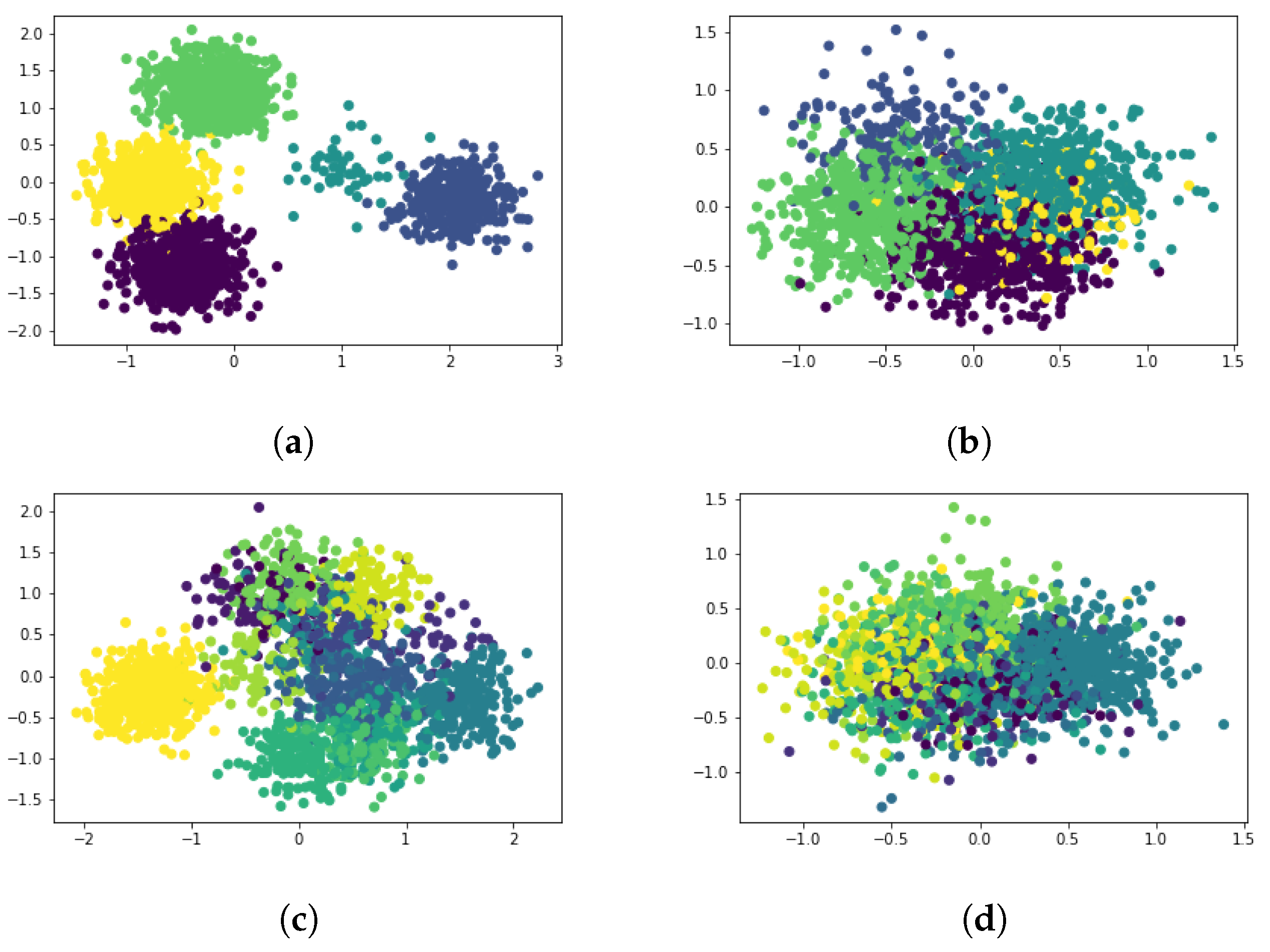
We applied the mechanism proposed in [66], which was later used in various papers, for instance [67,68,69], to generate our synthetic data. In this mechanism, first, we needed to determine the number of data points N, clusters K, and features V. Next, the clusters’ cardinalities were determined randomly with two constraints: (a) no cluster should contain less than a pre-specified number of data points (we set this number to 30 in our experiments), and (b) the number of data points in all clusters should sum to N. Once the cluster cardinalities were determined, we generated each cluster from a multivariate normal distribution whose covariance matrix was diagonal with diagonal values derived uniformly at random from the range $[0.05,0.1]$—they specify the cluster’s spread. We generated each component of the cluster centroid uniformly random from the range $\zeta [-1,+1]$, where $\zeta \in A$ controls the cluster intermix: the smaller value of $\zeta$, the higher the chance that data points from a cluster fall within the spreads of other clusters. Figure 3 depicts four examples of the generated datasets with $V=10$ for $\zeta =0.35$ and $\zeta =0.95$ for $N=2000$. The upper row visualizes five clusters, whereas the lower row shows 15 clusters.

As mentioned earlier, we generated synthetic data for two purposes: (A) to scrutinize the impact of the hyperparameters of our proposed methods and (B) to validate and compare the performance of our methods with other works from the literature. Concerning objective (A), with $N=2000$ and $V=10$, we generated datasets for two numbers of clusters $k=5,10$ and three distinct cluster intermix probabilities $\zeta =0.35,0.65,0.95$. These (synthetic data generator’s) settings led to six configurations as summarized in

Table 1. Synthetic datasets configurations to study the hyperparameters of proposed methods (six configurations) and to validate and compare the methods under consideration (72 configurations): each case consists of 10 repeats summing up to 780 datasets.

Generator Parameters	Hyperparameter-Scrutinizing Values	Comparison Values
Clusters (K)	5, 15	2, 10, 20
Features (V)	10	2, 5, 10, 15, 20, 200
Data points (N)	2000	1000, 3000
Clusters intermix ($\zeta$)	0.35, 0.65, 0.95	0.4, 0.8

. We repeated each configuration ten times, yielding 60 distinct datasets. We referred to these datasets as “hyperparameter-scrutinizing data.” Concerning objective (B), we studied the performance of methods under consideration for different numbers of clusters $K=2,10,20$, numbers of features $V=2,5,10,15,20,200$, data points $N=1000,3000$ and cluster intermix probabilities $\zeta =0.4,0.8$, as summarized in Table 1. These settings led to 72 configurations, each repeated ten times, yielding 720 distinct synthetic datasets. We called these datasets as “comparison data”. We ran each method with ten random seed initializations and chose the one that led to the best cluster inertia; then, we reported the averages and standard deviations of ten datasets of each configuration.

4.2.2. Real-World Data

We used 11 real-world datasets to validate and compare the performance of the methods under consideration. We downloaded ten datasets from the popular UCI Machine Learning repository [70] and the Chernoff Fossile dataset from [71]. We summarized the characteristics of these datasets in

Table 2. The real-world dataset’s characteristics.

Dataset	Points	Features	Clusters
Breast Tissue	106	9	6
Ecoli	336	7	8
Fossil	87	6	3
Glass	214	9	6
Iris	150	4	3
Leaf	340	15	30
Libras Movement	360	90	15
Optical Recognition	3823	62	10
Spam Base	4601	57	2
Pen-Based Recognition	7494	16	10
Wine	178	13	3

.

4.3. Evaluation Metric

We assess the performance of the clustering methods utilizing the normalized mutual information, NMI [72]. The NMI is a popular metric based on the concept of entropy to quantify the similarity between the cluster recovery results, $S={\left\{S_k\right\}}_{k=1}^K$, and the ground truth $T={\left\{T_l\right\}}_{l=1}^L$. Concretely, given S and T, NMI relies on the so-called contingency table, a two-way table whose rows correspond to components $S_k$ ($k=1,2,\dots ,K$) of S, and the columns correspond to components $T_l$ ($l=1,2,\dots ,L$) of T, such that its ($k,l$)-th entry is $n_{kl}=|S_k\cap T_l|$. The marginal row and marginal column, in respect, are defined as $a_k={\sum }_{l=1}^L{n}_{kl}=\left|S_k\right|$ and $b_l={\sum }_{k=1}^K{n}_{kl}=\left|T_l\right|$. The probability that an object picked at random falls into $S_k$ is $a\left(k\right)=a_k/N$. Similarly, the probability that an object picked at random falls into $T_l$ is $b\left(l\right)=b_l/N$. Therefore, we define the entropy of S as $H\left(S\right)=-{\sum }_{k=1}^{K}a\left(k\right)\log \left(a\right(k\left)\right)$. Similarly, we define $H\left(T\right)=-{\sum }_{l=1}^{L}b\left(l\right)\log \left(b\right(l\left)\right)$ as the entropy of T. Thus, the mutual information (MI) between S and T is calculated using:

$$MI\left(S,T\right)=\sum _k^K\sum _{l=1}^L{p}_{kl}\log (\frac{p_{kl}}{a\left(k\right)\times b\left(l\right))}),$$

(9)

where $p_{kl}=n_{kl}/N$ is the probability that an object picked at random falls into both $S_k$ and $T_l$ ($k=1,2,\dots ,K;l=1,2,\dots ,L$). Therefore, normalized mutual information is defined as

$$NMI=\frac{MI\left(S,T\right)}{max\left(H\right(S),H(T\left)\right)}.$$

(10)

For the NMI $\in [0,1]$, the closer its values are to one, the better the match between the clustering results and the ground truth and vice versa.

4.4. Data Pre-Processing

To pre-process the data, we used the so-called Min–Max standardization technique. Let $X={\left\{x_{iv}\right\}}_{i=1}^N$ for $v=1,\dots ,V$, where V is the number of features, represent the dataset. In addition, let $x_{va}$ and $x_{vb}$ represent the minimum and maximum of feature v for the entire dataset. The Min–Max method standardizes the data point $\widehat{x_{iv}}=\frac{x_{iv}-x_{va}}{x_{vb}-x_{va}}$ such that $\widehat{x_{iv}}\in [0,1]$. Although it was empirically shown, for instance in [67], that the clustering result might differ depending on how the data were standardized, due to the intuitiveness of the output of the Min–Max technique, we chose it as the default for our experiments.

5. Scrutinizing the Hyperparameters of the NGDC Method

Our proposed method contains two hyperparameters: (i) step size $\alpha$ and (ii) momentum decay coefficient ${\beta }_1$. Moreover, similar to other gradient-descent-based algorithms, the convergence of NGDC and its sensitivity to random seed initialization needed to be scrutinized. Consequently, we designed our hyperparameter-scrutinizing datasets, consisting of 60 synthetic data configurations, and summarized them in

Table 3. The hyperparameters’ search space of the proposed methods.

Hyperparameters	Values
Seed initialization	1, 5, 10, 20
Step size ($\alpha$)	0.0001, 0.001, 0.01, 0.1, 0.2, 0.5
Number of Iterations (T)	5, 10, 20, 40
Momentum decay (${\beta }_1$)	$0.01,0.1,0.3,0.6,0.9,0.99$
Minkowski p-values	1, 1.5, 2, 2.5, 3, 3.5, 4

to scrutinize these four items empirically.

5.1. Random Seed Initialization

The NGDC method is non-deterministic, implying that different seed initializations lead to different results. In supervised learning, where the evaluation of results due to the existence of ground truth is easily feasible, it is recommended to apply the (non-deterministic) algorithm under consideration with different random seed initializations and select the one which leads to more desirable results. Although in clustering there is no ground truth available, still, this framework can be applied by considering the value of the clustering criteria or any other accessible external source of information to evaluate the results. In this work, our goal was to scrutinize the hyperparameters and validate our proposed method empirically. Thus, we ran the NGDC method with the hyperparameter-scrutinizing data with four different numbers of random seed initialization, $n\_init$, and reported the results concerning the NMI in

Table 4. Studying the impact of different seed initialization using NMI values at fixed $\alpha =0.01$, ${\beta }_1=0.45$ and the maximum number of iterations equal to ten.

K	$\mathit{\zeta }$	$\mathit{n}\_\mathit{init}=1$	$\mathit{n}\_\mathit{init}=5$	$\mathit{n}\_\mathit{init}=10$	$\mathit{n}\_\mathit{init}=20$
5	0.35	0.540 ± 0.052	0.561 ± 0.055	0.567 ± 0.054	0.571 ± 0.056
	0.65	0.714 ± 0.075	0.758 ± 0.076	0.856 ± 0.063	0.886 ± 0.062
	0.95	0.851 ± 0.074	0.944 ± 0.068	0.963 ± 0.049	0.993 ± 0.010
15	0.35	0.400 ± 0.046	0.412 ± 0.050	0.413 ± 0.049	0.417 ± 0.048
	0.65	0.815 ± 0.032	0.839 ± 0.024	0.848 ± 0.033	0.863 ± 0.029
	0.95	0.898 ± 0.030	0.930 ± 0.015	0.948 ± 0.012	0.953 ± 0.009

.

The reported results of this table strongly suggest repeating the seed initialization at least five or ten times. Although the higher the number of seeds initialization, the better the performance of NGDC, still, the reported difference between 10 and 20 seeds initialization, in our opinion, is application-dependable. In addition, if the time has higher priority than accuracy, this difference can be neglected. In the rest of our computations, we use ten seeds initialization.

5.2. Convergence and the Number of Iterations

The convergence of gradient descent algorithms in the supervised learning tasks with random initialization has been well-studied and (under specific conditions) proved to be convergent; for instance, refer to [73,74] for more details. In our opinion, this subject deserves independent research devoted to clustering, and therefore, in the current study, relying upon the results of the two papers mentioned earlier, we limited our analyses to the impact of different numbers of iterations on the quality of the recovered clusters using the NMI values.

Relying on the number of iterations has its advantages and disadvantages. The main advantages are (i) not limiting the choice of the distance functions in the central loss function shown in Equation (1), and (ii) the termination of the NGDC is guaranteed. The disadvantages are that (i) the inappropriate number of iterations may lead NGDC to be stuck in local minima or pass a global minimum; and (ii) an external source of knowledge for assessing the quality of obtained results might be required for further adjustments.

Table 5. Studying the impact of different numbers of iterations using NMI at fixed $\alpha =0.01, {\beta }_1=0.45$ and 10 random seeds initializations.

K	$\mathit{\zeta }$	$\mathit{T}=1$	$\mathit{T}=5$	$\mathit{T}=10$	$\mathit{T}=20$	$\mathit{T}=40$
5	0.35	0.426 ± 0.045	0.567 ± 0.054	0.565 ± 0.055	0.567 ± 0.056	0.571 ± 0.055
	0.65	0.749 ± 0.076	0.838 ± 0.097	0.856 ± 0.063	0.779 ± 0.068	0.786 ± 0.079
	0.95	0.873 ± 0.043	0.974 ± 0.037	0.976 ± 0.043	0.973 ± 0.030	0.976 ± 0.035
15	0.35	0.315 ± 0.043	0.404 ± 0.051	0.418 ± 0.051	0.419 ± 0.048	0.423 ± 0.046
	0.65	0.716 ± 0.030	0.842 ± 0.026	0.848 ± 0.033	0.860 ± 0.027	0.869 ± 0.026
	0.95	0.864 ± 0.015	0.930 ± 0.013	0.953 ± 0.009	0.954 ± 0.013	0.961 ± 0.016

represents the results of our investigation on the number of iterations. Taking an attentive look at these results, one can conclude that in the majority of settings, the higher the number of iterations, the larger the value of NMI. However, except for one case, i.e., $(K=5, \zeta =0.65)$, in the rest of the cases, the improvement obtained by setting the number of iterations to more than 10 is insignificant (approximately less than $1\%$) and can be ignored. In our opinion, this exception (the second row) includes instances of the first disadvantage discussed earlier.

5.3. Step Size

Assuming that the loss function under consideration is convex and differentiable, i.e., its gradient is Lipschitz continuous with a constant L, it is not hard to prove its convergence. However, finding the constant L to adjust the proper step size is computationally expensive, and intuitively, numerical fine-tuning the step size has become a common practice in supervised learning. Following this convention, we studied the impact of the step size with the fixed number of iterations, in our case equal to ten, and applied NGDC to each dataset with ten different seeds.

We reported the results of our investigations to fine-tune the step size in

Table 6. Study of step size ($\alpha$) with fixed $n\_init=max\_iter=10$, $\mu =0.9$ and p-value = 2. The best results are bold-faced.

Configuration		$\mathit{\alpha }=0.0001$	$\mathit{\alpha }=0.001$	$\mathit{\alpha }=0.01$	$\mathit{\alpha }=0.1$	$\mathit{\alpha }=0.2$
K	$\mathit{\zeta }$	NMI	NMI	NMI	NMI	NMI
5	0.35	0.342 ± 0.060	0.524 ± 0.057	0.539 ± 0.052	0.003 ± 0.002	0.000 ± 0.000
	0.65	0.734 ± 0.078	0.806 ± 0.088	0.766 ± 0.063	0.005 ± 0.003	0.000 ± 0.000
	0.95	0.885 ± 0.062	0.950 ± 0.034	0.990 ± 0.011	0.004 ± 0.001	0.000 ± 0.000
15	0.35	0.287 ± 0.039	0.344 ± 0.045	0.388 ± 0.048	0.006 ± 0.007	0.000 ± 0.000
	0.65	0.666 ± 0.038	0.770 ± 0.026	0.844 ± 0.036	0.008 ± 0.008	0.000 ± 0.000
	0.95	0.840 ± 0.020	0.913 ± 0.018	0.953 ± 0.017	0.015 ± 0.008	0.000 ± 0.000

. From these results, it is not hard to conclude that the appropriate step size should be set to $0.01$.

5.4. NGDC Update Rule: ${\beta }_1$

We scrutinized and recorded the impact of the momentum (${\beta }_1$) in the NGDC update rule in

Table 7. Study of ${\beta }_1$ with fixed step size = $\alpha =0.01$, $n\_init=max\_iter=10$ and p-value = 2. The best results are bold-faced.

Configuration		${\mathit{\beta }}_1=0.01$	${\mathit{\beta }}_1=0.1$	${\mathit{\beta }}_1=0.3$	${\mathit{\beta }}_1=0.6$	${\mathit{\beta }}_1=0.9$	${\mathit{\beta }}_1=0.99$
K	$\mathit{\zeta }$	NMI	NMI	NMI	NMI	NMI	NMI
5	0.35	0.568 ± 0.054	0.568 ± 0.055	0.570 ± 0.054	0.562 ± 0.056	0.539 ± 0.039	0.005 ± 0.001
	0.65	0.792 ± 0.072	0.785 ± 0.054	0.837 ± 0.102	0.804 ± 0.090	0.766 ± 0.063	0.013 ± 0.008
	0.95	0.975 ± 0.032	0.960 ± 0.048	0.953 ± 0.052	0.992 ± 0.009	0.990 ± 0.011	0.011 ± 0.005
15	0.35	0.418 ± 0.053	0.417 ± 0.049	0.417 ± 0.049	0.416 ± 0.048	0.388 ± 0.048	0.025 ± 0.001
	0.65	0.844 ± 0.031	0.850 ± 0.038	0.849 ± 0.028	0.850 ± 0.029	0.844 ± 0.036	0.028 ± 0.002
	0.95	0.951 ± 0.014	0.955 ± 0.018	0.947 ± 0.012	0.943 ± 0.018	0.953 ± 0.017	0.029 ± 0.002

. As one can see, unlike the recommended value for this hyperparameter in classification tasks, usually $0.9$, here smaller values of ${\beta }_1$, specifically in more challenging datasets, lead to better cluster recovery results. Since there is no clear-cut edge between $0.3$ and $0.6$, we suggested fixing the default value to $0.045$.

5.5. Tuned Parameters

In this section, we empirically scrutinized the impact of different hyperparameters of the NGDC method to propose the default values. Considering our experimental results, we propose the following default values: (i) the step size $\alpha =0,01$; (ii) the momentum decay coefficient, ${\beta }_1$, for any value in the range $[0.3,0.6]$, we fixed it to $0.45$; (iii) the number of seeds initialization, $n\_init=10$; and (iv) the number of iterations, $T=10$.

It ought to be mentioned that not only our proposed methods but also some of our competitors can adopt different distance functions. For instance, the K-means clustering with cosine distance has proven to be an efficient alternative to the innate Euclidean distance as reported in [75]. However, to maintain a fair comparison in the rest of our computations, we fixed $p=2$ that imitates the innate Euclidean distance in the majority of the clustering methods.

5.6. p-Value in Minkowski Distance

As mentioned earlier, one of the contributions of our proposed method and our software implementation is its flexibility for accepting any differentiable distance function. We used the Minkowski distance with p-values bounded in $\left[1.0,4.0\right]$ and ran the NGDC method at the hyperparameter-scrutinizing datasets to demonstrate this advantage. We reported the corresponding results in

Table 8. Study of p-value with fixed step size $\alpha =0.01$, $n\_init=10$, ${\beta }_1=0.9$ and $max\_iter=10$. The best results are bold-faced.

Configuration		$\mathit{P}=1$	$\mathit{P}=1.5$	$\mathit{P}=2$	$\mathit{P}=2.5$	$\mathit{P}=3$	$\mathit{P}=3.5$	$\mathit{P}=4$
K	$\mathit{\zeta }$	NMI	NMI	NMI	NMI	NMI	NMI	NMI
5	0.35	0.056 ± 0.020	0.449 ± 0.060	0.544 ± 0.056	0.537 ± 0.057	0.504 ± 0.064	0.458 ± 0.068	0.391 ± 0.063
	0.65	0.353 ± 0.076	0.775 ± 0.091	0.806 ± 0.065	0.849 ± 0.082	0.840 ± 0.092	0.816 ± 0.070	0.772 ± 0.047
	0.95	0.705 ± 0.109	0.982 ± 0.019	0.970 ± 0.044	0.974 ± 0.032	0.953 ± 0.044	0.945 ± 0.038	0.942 ± 0.028
15	0.35	0.109 ± 0.014	0.340 ± 0.047	0.384 ± 0.051	0.376 ± 0.048	0.344 ± 0.043	0.312 ± 0.040	0.285 ± 0.035
	0.65	0.360 ± 0.055	0.826 ± 0.033	0.848 ± 0.033	0.834 ± 0.037	0.793 ± 0.035	0.750 ± 0.042	0.676 ± 0.039
	0.95	0.686 ± 0.047	0.953 ± 0.010	0.949 ± 0.016	0.936 ± 0.016	0.916 ± 0.021	0.895 ± 0.014	0.854 ± 0.028

.

From Table 8, one can observe that not only p-value equal to $1.5$ in two configurations has an edge over the others, but also the $p=2.5$ led to winning the competition when the cluster overlap probability is equal to $0.65$ and there were five clusters.

6. Experiments

6.1. Experimental Results at Real-World Data

We reported the comparison results of the methods under consideration using 11 real-world datasets in

Table 9. Comparison on real-world datasets with $n\_init=10$. The best results regarding NMI are bold-faced.

	K-Means	GMM	Spectral	Agglomerative	NGDC
Breast Tissue	0.515 ± 0.020	0.381 ± 0.047	0.462 ± 0.030	0.419 ± 0.000	0.549 ± 0.017
Ecoli	0.599 ± 0.010	0.388 ± 0.061	0.559 ± 0.007	0.667 ± 0.000	0.630 ± 0.024
Fossil	1.000 ± 0.000	0.687 ± 0.242	1.000 ± 0.000	1.000 ± 0.000	1.000 ± 0.000
Glass	0.338 ± 0.018	0.331 ± 0.035	0.277 ± 0.001	0.294 ± 0.000	0.387 ± 0.031
Iris	0.742 ± 0.000	0.629 ± 0.032	0.658 ± 0.000	0.784 ± 0.000	0.766 ± 0.020
Leaf	0.648 ± 0.010	0.589 ± 0.013	0.622 ± 0.017	0.621 ± 0.000	0.653 ± 0.009
Libras Movement	0.597 ± 0.015	0.197 ± 0.019	0.563 ± 0.016	0.563 ± 0.000	0.602 ± 0.012
Optical Recognition	0.761 ± 0.011	0.387 ± 0.068	0.699 ± 0.001	0.733 ± 0.000	0.774 ± 0.019
Spam Base	0.085 ± 0.115	0.080 ± 0.043	0.004 ± 0.000	0.001 ± 0.000	0.259 ± 0.003
Pen-Based Recognition	0.692 ± 0.006	0.691 ± 0.034	0.692 ± 0.000	0.635 ± 0.000	0.708 ± 0.010
Wine	0.846 ± 0.006	0.332 ± 0.107	0.909 ± 0.000	0.018 ± 0.000	0.858 ± 0.012

. Considering the number of wins, the NGDC won eight competitions, which turned it into the overall winner. Agglomerative clustering, by winning three competitions, can be considered the second winner.

We ought to highlight the following intriguing observations about NGDC performance: (i) it won in approximately $73\%$ of the real-world data; (ii) it obtained a relatively acceptable NMI equal to $0.55$ at the breast tissue dataset which is approximately $4\%$ higher than its closest competitor; (iii) similarly, using the glass dataset, it outperforms its closest competitor with approximately $5\%$ better NMI; (iv) except for NGDC, which obtained a poor NMI value equal to $0.26$, the rest of the methods under consideration failed to detect the clusters in the spam dataset. All these observations can be considered as pieces of evidence for the robustness and effectiveness of our proposed method. Nevertheless, we should emphasize that spectral clustering has a significant edge over its closest competitor, NGDC, in the wine dataset. More interestingly, except for GMM, the rest of the methods performed faultlessly on the Fossil dataset.

6.2. Experimental Results Using Synthetic Data

In this section, we compared the performance of our proposed methods with four popular and effective clustering methods described in Section 4.1 using our comparison datasets as outlined in the second half of Table 1.

We summarized the methods’ performance for the case of two clusters with 1000 and 3000 data points in

Table 10. Comparison on synthetic datasets with 1000 data points and two clusters. The best results regarding NMI are bold-faced.

V	$\mathit{\zeta }$	K-Means	GMM	Spectral	Agglomerative	NGDC
2	0.40	0.257 ± 0.212	0.041 ± 0.050	0.255 ± 0.215	0.008 ± 0.011	0.284 ± 0.200
	0.80	0.487 ± 0.286	0.075 ± 0.119	0.484 ± 0.282	0.180 ± 0.354	0.499 ± 0.286
5	0.40	0.538 ± 0.156	0.044 ± 0.059	0.537 ± 0.159	0.064 ± 0.184	0.523 ± 0.195
	0.80	0.876 ± 0.137	0.106 ± 0.087	0.877 ± 0.138	0.581 ± 0.474	0.837 ± 0.201
10	0.40	0.562 ± 0.151	0.415 ± 0.145	0.627 ± 0.138	0.006 ± 0.007	0.685 ± 0.175
	0.80	0.987 ± 0.033	0.976 ± 0.066	0.990 ± 0.024	0.895 ± 0.295	0.993 ± 0.009
15	0.40	0.869 ± 0.072	0.754 ± 0.294	0.883 ± 0.063	0.268 ± 0.399	0.882 ± 0.066
	0.80	1.000 ± 0.000	0.902 ± 0.293	1.000 ± 0.000	0.999 ± 0.003	1.000 ± 0.000
20	0.40	0.951 ± 0.039	0.310 ± 0.434	0.950 ± 0.037	0.281 ± 0.428	0.958 ± 0.033
	0.80	1.000 ± 0.000	1.000 ± 0.000	0.993 ± 0.008	0.997 ± 0.010	1.000 ± 0.000
200	0.40	1.000 ± 0.000	0.000 ± 0.000	0.992 ± 0.016	1.000 ± 0.000	0.600 ± 0.490
	0.80	1.000 ± 0.000	0.001 ± 0.001	1.000 ± 0.000	1.000 ± 0.000	1.000 ± 0.000

and

Table 11. Comparison on synthetic datasets with 3000 data points and two clusters. The best results regarding NMI are bold-faced.

V	$\mathit{\zeta }$	K-Means	GMM	Spectral	Agglomerative	NGDC
2	0.40	0.306 ± 0.200	0.168 ± 0.112	0.306 ± 0.199	0.001 ± 0.001	0.313 ± 0.201
	0.80	0.584 ± 0.261	0.107 ± 0.104	0.574 ± 0.255	0.249 ± 0.381	0.589 ± 0.260
5	0.40	0.395 ± 0.230	0.033 ± 0.047	0.391 ± 0.228	0.002 ± 0.004	0.403 ± 0.224
	0.80	0.844 ± 0.140	0.339 ± 0.276	0.858 ± 0.135	0.463 ± 0.465	0.852 ± 0.141
10	0.40	0.750 ± 0.165	0.015 ± 0.014	0.748 ± 0.165	0.089 ± 0.264	0.757 ± 0.165
	0.80	0.969 ± 0.064	0.028 ± 0.030	0.970 ± 0.062	0.884 ± 0.294	0.972 ± 0.061
15	0.40	0.835 ± 0.111	0.018 ± 0.014	0.834 ± 0.109	0.001 ± 0.001	0.843 ± 0.108
	0.80	1.000 ± 0.000	0.118 ± 0.295	0.999 ± 0.002	0.998 ± 0.004	1.000 ± 0.000
20	0.40	0.918 ± 0.069	0.844 ± 0.283	0.926 ± 0.061	0.095 ± 0.280	0.922 ± 0.073
	0.80	0.999 ± 0.004	1.000 ± 0.000	0.994 ± 0.007	1.000 ± 0.000	0.999 ± 0.004
200	0.40	1.000 ± 0.000	0.001 ± 0.001	1.000 ± 0.000	1.000 ± 0.000	1.000 ± 0.000
	0.80	1.000 ± 0.000	0.000 ± 0.000	1.000 ± 0.000	1.000 ± 0.000	1.000 ± 0.000

, respectively. In both tables, NGDC, with slightly better results compared to its closest competitors, can be considered the overall winner. However, its unstable performance in Table 10 with 200 features and $\zeta =0.4$, leading to NMI equal to $0.6$ with a high standard deviation of $0.49$, might require further investigations. The K-means and spectral clusterings each won eight settings in the total of both tables and can be considered the second winners. Moreover, considering the overall performances of methods, one may consider the settings with two features as the most challenging, especially when $\zeta =0.4$ and $V=200$ as the most straightforward. However, surprisingly, the GMM failed even in such simple settings, and except for a couple of other simple settings, i.e., $\zeta =0.8$, the GMM performed poorly. Although the agglomerative also did not perform encouragingly in most settings, it still performed better than GMM.

We reported the results of methods under consideration with ten clusters and 1000 data points in

Table 12. Comparison on synthetic datasets with 1000 data points and ten clusters. The best results regarding NMI are bold-faced.

V	$\mathit{\zeta }$	K-Means	GMM	Spectral	Agglomerative	NGDC
2	0.40	0.207 ± 0.040	0.157 ± 0.045	0.193 ± 0.039	0.192 ± 0.039	0.212 ± 0.040
	0.80	0.432 ± 0.041	0.321 ± 0.077	0.401 ± 0.030	0.433 ± 0.038	0.438 ± 0.043
5	0.40	0.350 ± 0.049	0.200 ± 0.045	0.285 ± 0.026	0.199 ± 0.081	0.358 ± 0.046
	0.80	0.753 ± 0.044	0.607 ± 0.077	0.641 ± 0.061	0.711 ± 0.063	0.751 ± 0.042
10	0.40	0.549 ± 0.077	0.283 ± 0.072	0.460 ± 0.077	0.251 ± 0.153	0.546 ± 0.075
	0.80	0.957 ± 0.029	0.765 ± 0.083	0.922 ± 0.037	0.925 ± 0.027	0.956 ± 0.025
15	0.40	0.757 ± 0.050	0.338 ± 0.057	0.677 ± 0.075	0.363 ± 0.196	0.739 ± 0.045
	0.80	0.940 ± 0.030	0.666 ± 0.051	0.991 ± 0.011	0.985 ± 0.023	0.948 ± 0.031
20	0.40	0.862 ± 0.034	0.316 ± 0.016	0.804 ± 0.031	0.566 ± 0.125	0.843 ± 0.035
	0.80	0.993 ± 0.015	0.676 ± 0.051	0.999 ± 0.002	0.999 ± 0.002	0.970 ± 0.014
200	0.40	0.971 ± 0.027	0.023 ± 0.003	1.000 ± 0.000	1.000 ± 0.000	0.916 ± 0.020
	0.80	0.961 ± 0.027	0.023 ± 0.003	1.000 ± 0.000	1.000 ± 0.000	0.930 ± 0.027

, and we show the results of data with 3000 data points and the same number of clusters in

Table 13. Comparison on synthetic datasets with 3000 data points and ten clusters. The best results regarding NMI are bold-faced.

V	$\mathit{\zeta }$	K-Means	GMM	Spectral	Agglomerative	NGDC
2	0.40	0.200 ± 0.031	0.158 ± 0.041	0.193 ± 0.029	0.189 ± 0.035	0.204 ± 0.033
	0.80	0.410 ± 0.052	0.346 ± 0.081	0.381 ± 0.046	0.415 ± 0.062	0.413 ± 0.052
5	0.40	0.348 ± 0.054	0.199 ± 0.056	0.283 ± 0.041	0.169 ± 0.101	0.355 ± 0.053
	0.80	0.716 ± 0.057	0.685 ± 0.138	0.604 ± 0.055	0.743 ± 0.062	0.730 ± 0.066
10	0.40	0.579 ± 0.046	0.327 ± 0.132	0.484 ± 0.049	0.032 ± 0.045	0.581 ± 0.042
	0.80	0.920 ± 0.035	0.892 ± 0.041	0.877 ± 0.042	0.901 ± 0.045	0.927 ± 0.021
15	0.40	0.714 ± 0.051	0.552 ± 0.113	0.616 ± 0.050	0.178 ± 0.218	0.727 ± 0.057
	0.80	0.935 ± 0.031	0.909 ± 0.078	0.967 ± 0.039	0.990 ± 0.008	0.922 ± 0.034
20	0.40	0.852 ± 0.031	0.635 ± 0.067	0.784 ± 0.036	0.352 ± 0.263	0.845 ± 0.036
	0.80	0.956 ± 0.025	0.834 ± 0.086	0.999 ± 0.001	0.998 ± 0.001	0.967 ± 0.019
200	0.40	0.979 ± 0.014	0.011 ± 0.001	1.000 ± 0.000	1.000 ± 0.000	0.940 ± 0.018
	0.80	0.974 ± 0.022	0.015 ± 0.003	1.000 ± 0.000	1.000 ± 0.000	0.970 ± 0.008

. Concerning the number of wins, the NGDC and agglomeration each, in total, won eight settings and thus can be considered the joint winners. However, it ought to be highlighted that four out of eight wins of agglomerative clustering were obtained using the most straightforward datasets (the last two rows). Whilst NGDC also obtained completely acceptable results, it stocked at a local minimum in some cases. The closeness of NGDC results to the winners in the cases for which it did not win, for instance, $N=1000,V=5,10$, can also be considered another piece of evidence for its effectiveness. The spectral and K-means clusterings, in respect, are the second and third winners. The GMM still performs poorly; however, it is slightly better than the case of the existence of two clusters.

We represented the methods’ results for the case of 20 clusters with 1000 and 3000 data points in

Table 14. Comparison on synthetic datasets with 1000 data points and 20 clusters. The best results regarding NMI are bold-faced.

V	$\mathit{\zeta }$	K-Means	GMM	Spectral	Agglomerative	NGDC
2	0.40	0.217 ± 0.023	0.160 ± 0.028	0.191 ± 0.025	0.207 ± 0.025	0.220 ± 0.022
	0.80	0.402 ± 0.028	0.333 ± 0.027	0.378 ± 0.024	0.403 ± 0.033	0.408 ± 0.027
5	0.40	0.325 ± 0.027	0.225 ± 0.026	0.286 ± 0.020	0.252 ± 0.029	0.328 ± 0.023
	0.80	0.697 ± 0.048	0.513 ± 0.078	0.601 ± 0.043	0.653 ± 0.047	0.683 ± 0.043
10	0.40	0.494 ± 0.043	0.271 ± 0.017	0.424 ± 0.040	0.307 ± 0.046	0.477 ± 0.029
	0.80	0.928 ± 0.020	0.689 ± 0.020	0.914 ± 0.018	0.904 ± 0.024	0.911 ± 0.017
15	0.40	0.702 ± 0.031	0.350 ± 0.017	0.631 ± 0.026	0.459 ± 0.059	0.643 ± 0.025
	0.80	0.968 ± 0.013	0.717 ± 0.039	0.974 ± 0.016	0.979 ± 0.012	0.949 ± 0.019
20	0.40	0.837 ± 0.023	0.376 ± 0.021	0.793 ± 0.029	0.617 ± 0.037	0.768 ± 0.035
	0.80	0.968 ± 0.009	0.708 ± 0.023	0.999 ± 0.001	0.999 ± 0.001	0.959 ± 0.013
200	0.40	0.963 ± 0.009	0.082 ± 0.008	1.000 ± 0.000	1.000 ± 0.000	0.900 ± 0.017
	0.80	0.973 ± 0.006	0.083 ± 0.007	1.000 ± 0.000	1.000 ± 0.000	0.926 ± 0.014

and

Table 15. Comparison on synthetic datasets with 3000 data points and 20 clusters. The best results regarding NMI are bold-faced.

V	$\mathit{\zeta }$	K-Means	GMM	Spectral	Agglomerative	NGDC
2	0.40	0.179 ± 0.024	0.148 ± 0.026	0.174 ± 0.023	0.176 ± 0.022	0.182 ± 0.023
	0.80	0.390 ± 0.042	0.342 ± 0.055	0.373 ± 0.043	0.392 ± 0.045	0.394 ± 0.042
5	0.40	0.298 ± 0.042	0.199 ± 0.039	0.264 ± 0.038	0.218 ± 0.060	0.303 ± 0.042
	0.80	0.691 ± 0.025	0.462 ± 0.083	0.581 ± 0.031	0.648 ± 0.044	0.689 ± 0.026
10	0.40	0.486 ± 0.040	0.282 ± 0.059	0.396 ± 0.031	0.220 ± 0.057	0.482 ± 0.041
	0.80	0.919 ± 0.016	0.835 ± 0.029	0.889 ± 0.024	0.894 ± 0.030	0.922 ± 0.025
15	0.40	0.686 ± 0.037	0.433 ± 0.044	0.586 ± 0.045	0.258 ± 0.159	0.670 ± 0.034
	0.80	0.913 ± 0.016	0.870 ± 0.034	0.937 ± 0.023	0.983 ± 0.011	0.914 ± 0.016
20	0.40	0.797 ± 0.021	0.480 ± 0.045	0.728 ± 0.037	0.538 ± 0.087	0.787 ± 0.027
	0.80	0.975 ± 0.010	0.815 ± 0.043	0.996 ± 0.005	0.997 ± 0.003	0.961 ± 0.005
200	0.40	0.960 ± 0.013	0.046 ± 0.002	0.999 ± 0.001	1.000 ± 0.000	0.917 ± 0.016
	0.80	0.960 ± 0.019	0.061 ± 0.005	1.000 ± 0.000	1.000 ± 0.000	0.938 ± 0.017

, respectively. Now, the K-means, by winning nine settings, is the winner, and the agglomerative and NGDC, in respect, by winning eight and seven settings, are the second and third winners, respectively. Similar to the previous observations, we noticed similar patterns in the performance of the NGDC and agglomerative clustering concerning the relationship between data complexity and the quality of the obtained results. We also observed similar results with subtle improvements in the performances of spectral and GMM clustering methods.

It is noteworthy to mention that we ran NGDC with $T=20$ and $T=40$; however, since these increases in the number of iterations, as expected, did not lead to significant improvements, we did not report those results.

7. Conclusions and Future Work

In this work, we proposed a generic clustering criterion and adopted the GD algorithm to optimize it; our unreported experiments were aligned with the well-known fact that the Vanilla GD is prone to slow convergence, especially at nearly flat surfaces. Consequently, inspired by the Nesterov momentum, we proposed the NGDC method. As a by-product of our proposed method, we implemented the NGDC using Jax (an automatic differentiation library).

The NGDC method contains two hyperparameters: (i) step size $\alpha$ and (ii) momentum decay coefficient ${\beta }_1$. Similar to other gradient-descent-based algorithms, the convergence of NGDC and its sensitivity to random seed initialization needed to be scrutinized. Consequently, we designed the hyperparameter-scrutinizing datasets consisting of 60 synthetic data configurations (refer Table 3) to study the items mentioned earlier empirically.

Our investigations on the impact of random seed initialization showed that exploiting five or ten random initializations is sufficient; therefore, in the rest of our computations, we set this parameter to ten. Next, we studied the convergence of NGDC. The convergence of gradient-descent-based algorithms is well-studied, and it is proven that all GD-based algorithms under a specific set of conditions are convergent: although we think this subject deserves a separate study devoted to gradient descent adopted for clustering, relying on the results of previous research, we limited the current study to establish a stopping condition, i.e., the relationship between convergence and the number of iterations. Our results demonstrated that usually, NGDC converges within ten iterations; therefore, in the rest of our computations, we used ten iterations.

Following, we analyzed the impact of step size and momentum decay coefficient using our hyperparameter-scrutinizing datasets. Our computations suggested that one can set the step size equal to $0.01$ and choose any values from the range $[0.3,0.6]$ for the momentum decay coefficient; we fixed ${\beta }_1=0.45$.

Furthermore, our experiments using hyperparameters-scrutinizing datasets showed that our flexible implementation of the NGDC enables users to adopt any differentiable distance function for further improvements of the cluster recovery results. More so, we demonstrated that there were cases in which setting the p-value of Minkowski distance to $1.5$ or $2.5$ led to higher NMI values than the innate $p=2$. One may consider these cases as preliminary pieces of evidence for a better scalability and generalization power of NGDC.

Once we fine-tuned the NGDC’s hyperparameters, we statistically validated and compared its performance with four clustering methods from the literature on 11 real-world and 720 synthetic datasets. In the real-world data competitions, the NGDC won approximately $73\%$ of the competitions, turning it into the prevailing winner when using real-world datasets. More so, for the breast tissue and glass datasets, in respect, it obtained approximately $4\%$ and $5\%$ higher NMI compared to its closest competitor, K-means. The performance of methods in the Spam and Fossile datasets needs to be highlighted. For the Fossile dataset, except for GMM with $NMI=0.69$, the rest of the methods recovered the clusters without any mistakes. Conversely, in the Spam dataset, except for NGDC with poor $NMI=0.26$, the rest of the methods failed to detect the clusters. Agglomerative clustering by winning three competitions and spectral clustering by winning two competitions are the second and third winners of real-world data competition.

Similar to real-world data competitions, in the synthetic data competitions, NGDC won 300 competitions and took first place. K-means won 230 datasets and took second place. Agglomerative and spectral clustering each won 210 competitions and jointly won third place. The GMM won only 20 competitions and performed poorly in most settings.

Taking a closer look at synthetic data results reveals the following points: (a) In general, we have three groups of algorithms. The first group consists of NGDC and K-means with frequently acceptable performance; the second group consists of spectral and agglomerative clusterings for which they usually performed acceptably on the settings with large number of features; and the third group contains GMM with frequent poor performances. (b) Although NGDC frequently performed acceptably; however, it constantly failed to recover completely faultless clusters when there were more than two clusters, and the number of features was equal to 200. In our opinion, these nuances in the performance of NGDC could occur due to convergence near the optimum, while the exhaustive search in the agglomeration clustering led to faultless recovery. (c) The reason for the constantly acceptable performance of the K-means might be because the underlying assumption of this algorithm and our synthetic data were both multivariate Gaussian distributions. (d) The performance of all methods under consideration in $V=2,\zeta =0.4,0.8$ and $V=5,\zeta =0.4$ settings were moderate or even poor. This issue can be tackled by using a more powerful model and the same algorithm.

The current research is not without drawbacks, and those drawbacks form some aspects of our future research as follows.

The central purpose of the current research was to improve the effectiveness of clustering methods, and thus, we proposed a generic clustering criterion and used the JAX library to implement it: with this setting, we equipped users with the possibility of applying a diverse range of (differentiable) distance functions and adjusting the hyperparameters depending on the data under consideration. Although we empirically studied the hyperparameters of NGDC and proposed some default values, and they proved to be effective, however, due to the “no free lunch theorem,” we believe developing a novel framework for employing NGDC in a semi-supervised manner can be a promising future direction.

Despite our endeavors in the current research, we failed to establish new convergence conditions and instead empirically scrutinized the impact number of iterations on the quality of recovered clusters. Theoretical analysis of NGDC convergence is another beneficial future direction. Furthermore, in the current research, we applied the Minkowski distance on our hyperparameter-scrutinizing data to demonstrate the possibility for further improvement in cluster recovery. However, we believe this subject needs a more rigorous investigation, and thus scrutinizing the impact of various distance metrics, including Minkowski metrics with different p-values, could be the third future direction.

Adopting other update rules such as RMSProb and ADAM can be considered our fourth direction. Reformulating our proposed clustering objective functions using a probabilistic approach so that we can determine the probability of clusters’ membership is another promising future direction. Last but not least, extending the NGDC method to more complex data structures, for instance, to the feature-rich networks [68], is another promising future area of research.

References

- Ezugwu, A.E.; Ikotun, A.M.; Oyelade, O.O.; Abualigah, L.; Agushaka, J.O.; Eke, C.I.; Akinyelu, A.A. A comprehensive survey of clustering algorithms: State-of-the-art machine learning applications, taxonomy, challenges, and future research prospects. Eng. Appl. Artif. Intell. 2022, 110, 104743. [Google Scholar] [CrossRef]
- Murphy, K.P. Probabilistic Machine Learning: An Introduction; MIT Press: Cambridge, MA, USA, 2022. [Google Scholar]
- Bradbury, J.; Frostig, R.; Hawkins, P.; Johnson, M.J.; Leary, C.; Maclaurin, D.; Necula, G.; Paszke, A.; VanderPlas, J.; Wanderman-Milne, S.; et al. JAX: Composable Transformations of Python+NumPy Programs. 2018. Available online: https://github.com/google/jax (accessed on 2 February 2018).
- Steinley, D. K-means clustering: A half-century synthesis. Br. J. Math. Stat. Psychol. 2006, 59, 1–34. [Google Scholar] [CrossRef] [PubMed] [Green Version]
- Van der Laan, M.; Pollard, K.; Bryan, J. A new partitioning around medoids algorithm. J. Stat. Comput. Simul. 2003, 73, 575–584. [Google Scholar] [CrossRef] [Green Version]
- Park, H.S.; Jun, C.H. A simple and fast algorithm for K-medoids clustering. Expert Syst. Appl. 2009, 36, 3336–3341. [Google Scholar] [CrossRef]
- Campello, R.J.; Kröger, P.; Sander, J.; Zimek, A. Density-based clustering. Wiley Interdiscip. Rev. Data Min. Knowl. Discov. 2020, 10, e1343. [Google Scholar] [CrossRef]
- Schubert, E.; Sander, J.; Ester, M.; Kriegel, H.P.; Xu, X. DBSCAN revisited, revisited: Why and how you should (still) use DBSCAN. ACM Trans. Database Syst. (TODS) 2017, 42, 1–21. [Google Scholar] [CrossRef]
- Ankerst, M.; Breunig, M.M.; Kriegel, H.P.; Sander, J. OPTICS: Ordering points to identify the clustering structure. ACM Sigmod Rec. 1999, 28, 49–60. [Google Scholar] [CrossRef]
- Schubert, E.; Gertz, M. Improving the Cluster Structure Extracted from OPTICS Plots. In Proceedings of the LWDA, Mannheim, Germany, 22–24 August 2018; pp. 318–329. [Google Scholar]
- Agrawal, R.; Gehrke, J.; Gunopulos, D.; Raghavan, P. Automatic subspace clustering of high dimensional data. Data Min. Knowl. Discov. 2005, 11, 5–33. [Google Scholar] [CrossRef] [Green Version]
- Mirjalili, S.; Lewis, A. The whale optimization algorithm. Adv. Eng. Softw. 2016, 95, 51–67. [Google Scholar] [CrossRef]
- Nasiri, J.; Khiyabani, F.M. A whale optimization algorithm (WOA) approach for clustering. Cogent Math. Stat. 2018, 5, 1483565. [Google Scholar] [CrossRef]
- Aliniya, Z.; Mirroshandel, S.A. A novel combinatorial merge-split approach for automatic clustering using imperialist competitive algorithm. Expert Syst. Appl. 2019, 117, 243–266. [Google Scholar] [CrossRef]
- Ezugwu, A.E. Nature-inspired metaheuristic techniques for automatic clustering: A survey and performance study. SN Appl. Sci. 2020, 2, 1–57. [Google Scholar] [CrossRef] [Green Version]
- Chollet, F. Deep Learning with Python; Simon and Schuster: New York, NY, USA, 2021. [Google Scholar]
- Murphy, K.P. Probabilistic Machine Learning: Advanced Topics; MIT Press: Cambridge, MA, USA, 2023. [Google Scholar]
- Min, E.; Guo, X.; Liu, Q.; Zhang, G.; Cui, J.; Long, J. A survey of clustering with deep learning: From the perspective of network architecture. IEEE Access 2018, 6, 39501–39514. [Google Scholar] [CrossRef]
- Zadeh, L.A. Fuzzy sets. Inf. Control 1965, 8, 338–353. [Google Scholar] [CrossRef] [Green Version]
- Saxena, A.; Prasad, M.; Gupta, A.; Bharill, N.; Patel, O.P.; Tiwari, A.; Er, M.J.; Ding, W.; Lin, C.T. A review of clustering techniques and developments. Neurocomputing 2017, 267, 664–681. [Google Scholar] [CrossRef] [Green Version]
- Yager, R.R.; Filev, D.P. Approximate clustering via the mountain method. IEEE Trans. Syst. Man Cybern. 1994, 24, 1279–1284. [Google Scholar] [CrossRef]
- Krishnapuram, R.; Keller, J.M. A possibilistic approach to clustering. IEEE Trans. Fuzzy Syst. 1993, 1, 98–110. [Google Scholar] [CrossRef]
- Shi, Z.; Wu, D.; Guo, C.; Zhao, C.; Cui, Y.; Wang, F.Y. FCM-RDpA: TSK fuzzy regression model construction using fuzzy C-means clustering, regularization, Droprule, and Powerball Adabelief. Inf. Sci. 2021, 574, 490–504. [Google Scholar] [CrossRef]
- Bouwmans, T.; Sobral, A.; Javed, S.; Jung, S.K.; Zahzah, E.H. Decomposition into low-rank plus additive matrices for background/foreground separation: A review for a comparative evaluation with a large-scale dataset. Comput. Sci. Rev. 2017, 23, 1–71. [Google Scholar] [CrossRef] [Green Version]
- Chowdhury, K.; Chaudhuri, D.; Pal, A.K. An entropy-based initialization method of K-means clustering on the optimal number of clusters. Neural Comput. Appl. 2021, 33, 6965–6982. [Google Scholar] [CrossRef]
- Verbeek, J. Mixture Models for Clustering and Dimension Reduction. Ph.D. Thesis, Universiteit van Amsterdam, Amsterdam, The Netherlands, 2004. [Google Scholar]
- McLachlan, G.J.; Rathnayake, S. On the number of components in a Gaussian mixture model. Wiley Interdiscip. Rev. Data Min. Knowl. Discov. 2014, 4, 341–355. [Google Scholar] [CrossRef]
- Murtagh, F.; Contreras, P. Algorithms for hierarchical clustering: An overview. Wiley Interdiscip. Rev. Data Min. Knowl. Discov. 2012, 2, 86–97. [Google Scholar] [CrossRef]
- Murtagh, F.; Contreras, P. Algorithms for hierarchical clustering: An overview, II. Wiley Interdiscip. Rev. Data Min. Knowl. Discov. 2017, 7, e1219. [Google Scholar] [CrossRef] [Green Version]
- Blashfield, R.K.; Aldenderfer, M.S. The literature on cluster analysis. Multivar. Behav. Res. 1978, 13, 271–295. [Google Scholar] [CrossRef]
- Sneath, P.H. Thirty years of numerical taxonomy. Syst. Biol. 1995, 44, 281–298. [Google Scholar] [CrossRef]
- Sneath, P.H.; Sokal, R.R. Numerical Taxonomy San Francisco. Stat. Method Eval. Syst. Relationsh. 1973, 38, 1409–1438. [Google Scholar]
- Ward, J.H., Jr. Hierarchical grouping to optimize an objective function. J. Am. Stat. Assoc. 1963, 58, 236–244. [Google Scholar] [CrossRef]
- Murtagh, F.; Legendre, P. Ward’s hierarchical agglomerative clustering method: Which algorithms implement Ward’s criterion? J. Classif. 2014, 31, 274–295. [Google Scholar] [CrossRef] [Green Version]
- Zhang, T.; Ramakrishnan, R.; Livny, M. BIRCH: An efficient data clustering method for very large databases. ACM SIGMOD Rec. 1996, 25, 103–114. [Google Scholar] [CrossRef]
- Boley, D. Principal direction divisive partitioning. Data Min. Knowl. Discov. 1998, 2, 325–344. [Google Scholar] [CrossRef]
- Savaresi, S.M.; Boley, D.L.; Bittanti, S.; Gazzaniga, G. Cluster selection in divisive clustering algorithms. In Proceedings of the 2002 SIAM International Conference on Data Mining, SIAM, Arlington, VA, USA, 11–13 April 2002; pp. 299–314. [Google Scholar]
- Chavent, M.; Lechevallier, Y.; Briant, O. DIVCLUS-T: A monothetic divisive hierarchical clustering method. Comput. Stat. Data Anal. 2007, 52, 687–701. [Google Scholar] [CrossRef] [Green Version]
- Karypis, G.; Kumar, V. Multilevel k-way hypergraph partitioning. In Proceedings of the 36th Annual ACM/IEEE Design Automation Conference, New Orleans, LA, USA, 21–25 June 1999; pp. 343–348. [Google Scholar]
- Zhong, C.; Miao, D.; Wang, R.; Zhou, X. DIVFRP: An automatic divisive hierarchical clustering method based on the furthest reference points. Pattern Recognit. Lett. 2008, 29, 2067–2077. [Google Scholar] [CrossRef]
- Feng, L.; Qiu, M.H.; Wang, Y.X.; Xiang, Q.L.; Yang, Y.F.; Liu, K. A fast divisive clustering algorithm using an improved discrete particle swarm optimizer. Pattern Recognit. Lett. 2010, 31, 1216–1225. [Google Scholar] [CrossRef]
- Williams, W.T.; Lambert, J.M. Multivariate methods in plant ecology: I. Association-analysis in plant communities. J. Ecol. 1959, 47, 83–101. [Google Scholar] [CrossRef]
- Kim, J.; Billard, L. Dissimilarity measures and divisive clustering for symbolic multimodal-valued data. Comput. Stat. Data Anal. 2012, 56, 2795–2808. [Google Scholar] [CrossRef]
- Kim, J.; Billard, L. A polythetic clustering process and cluster validity indexes for histogram-valued objects. Comput. Stat. Data Anal. 2011, 55, 2250–2262. [Google Scholar] [CrossRef]
- Kim, J.; Lee, W.; Song, J.J.; Lee, S.B. Optimized combinatorial clustering for stochastic processes. Clust. Comput. 2017, 20, 1135–1148. [Google Scholar] [CrossRef] [Green Version]
- Jenssen, R.; Erdogmus, D.; Hild, K.E., II; Principe, J.C.; Eltoft, T. Information cut for clustering using a gradient descent approach. Pattern Recognit. 2007, 40, 796–806. [Google Scholar] [CrossRef]
- Charytanowicz, M.; Niewczas, J.; Kulczycki, P.; Kowalski, P.A.; Łukasik, S.; Żak, S. Complete gradient clustering algorithm for features analysis of x-ray images. In Information Technologies in Biomedicine: Volume 2, Proceedings of the Information Technologies in Biomedicine ITiB, Kamien Slaski, Poland, 7–9 June 2010; Springer: Berlin/Heidelberg, Germany, 2010; pp. 15–24. [Google Scholar]
- Messaoud, S.; Bradai, A.; Moulay, E. Online GMM clustering and mini-batch gradient descent based optimization for industrial IoT 4.0. IEEE Trans. Ind. Inform. 2019, 16, 1427–1435. [Google Scholar] [CrossRef]
- Sculley, D. Web-scale k-means clustering. In Proceedings of the 19th International Conference on World Wide Web, Raleigh, NC, USA, 26–30 April 2010; pp. 1177–1178. [Google Scholar]
- Yin, P.; Pham, M.; Oberman, A.; Osher, S. Stochastic backward Euler: An implicit gradient descent algorithm for k-means clustering. J. Sci. Comput. 2018, 77, 1133–1146. [Google Scholar] [CrossRef] [Green Version]
- Wang, Y.; Chen, L.; Mei, J.P. Stochastic gradient descent based fuzzy clustering for large data. In Proceedings of the 2014 IEEE International Conference on Fuzzy Systems (FUZZ-IEEE), Luxembourg, 11–14 July 2014; pp. 2511–2518. [Google Scholar]
- Monath, N.; Zaheer, M.; Silva, D.; McCallum, A.; Ahmed, A. Gradient-based hierarchical clustering using continuous representations of trees in hyperbolic space. In Proceedings of the 25th ACM SIGKDD International Conference on Knowledge Discovery & Data Mining, Anchorage, AK, USA, 4–8 August 2019; pp. 714–722. [Google Scholar]
- Wong, C.C.; Chen, C.C. A hybrid clustering and gradient descent approach for fuzzy modeling. IEEE Trans. Syst. Man Cybern. Part B 1999, 29, 686–693. [Google Scholar] [CrossRef] [PubMed]
- Son, L.H.; Van Hai, P. A novel multiple fuzzy clustering method based on internal clustering validation measures with gradient descent. Int. J. Fuzzy Syst. 2016, 18, 894–903. [Google Scholar] [CrossRef]
- Mirkin, B. The iterative extraction approach to clustering. In Principal Manifolds for Data Visualization and Dimension Reduction; Springer: Berlin/Heidelberg, Germany, 2008; pp. 151–177. [Google Scholar]
- Mirkin, B. Clustering for Data Mining: A Data Recovery Approach; Chapman and Hall/CRC: Boca Raton, FL, USA, 2005. [Google Scholar]
- Mirkin, B.; Shalileh, S. Community Detection in Feature-Rich Networks Using Data Recovery Approach. J. Classif. 2022, 39, 432–462. [Google Scholar] [CrossRef]
- Kochenderfer, M.J.; Wheeler, T.A. Algorithms for Optimization; MIT Press: Cambridge, MA, USA, 2019. [Google Scholar]
- Wilson, D.R.; Martinez, T.R. The general inefficiency of batch training for gradient descent learning. Neural Netw. 2003, 16, 1429–1451. [Google Scholar] [CrossRef] [Green Version]
- Qian, N. On the momentum term in gradient descent learning algorithms. Neural Netw. 1999, 12, 145–151. [Google Scholar] [CrossRef]
- Nesterov, Y.E. A method of solving a convex programming problem with convergence rate O(1/k2). Proc. Dokl. Akad. Nauk. Russ. Acad. Sci. 1983, 269, 543–547. [Google Scholar]
- Duchi, J.; Hazan, E.; Singer, Y. Adaptive subgradient methods for online learning and stochastic optimization. J. Mach. Learn. Res. 2011, 12, 2121–2159. [Google Scholar]
- Kingma, D.P.; Ba, J. Adam: A method for stochastic optimization. arXiv 2014, arXiv:1412.6980. [Google Scholar]
- Zeiler, M.D. Adadelta: An adaptive learning rate method. arXiv 2012, arXiv:1212.5701. [Google Scholar]
- Von Luxburg, U. A tutorial on spectral clustering. Stat. Comput. 2007, 17, 395–416. [Google Scholar] [CrossRef]
- Kovaleva, E.V.; Mirkin, B.G. Bisecting K-means and 1D projection divisive clustering: A unified framework and experimental comparison. J. Classif. 2015, 32, 414–442. [Google Scholar] [CrossRef]
- Shalileh, S.; Mirkin, B. Least-squares community extraction in feature-rich networks using similarity data. PLoS ONE 2021, 16, e0254377. [Google Scholar] [CrossRef] [PubMed]
- Shalileh, S.; Mirkin, B. Community partitioning over feature-rich networks using an extended k-means method. Entropy 2022, 24, 626. [Google Scholar] [CrossRef] [PubMed]
- Shalileh, S.; Mirkin, B. Summable and nonsummable data-driven models for community detection in feature-rich networks. Soc. Netw. Anal. Min. 2021, 11, 1–23. [Google Scholar] [CrossRef]
- Dua, D.; Graff, C. UCI Machine Learning Repository. 2017. Available online: https://archive.ics.uci.edu/ml/index.php (accessed on 1 January 2007).
- Chernoff, H. The use of faces to represent points in k-dimensional space graphically. J. Am. Stat. Assoc. 1973, 68, 361–368. [Google Scholar] [CrossRef]
- Cover, T.; Thomas, J. Elements of Information Theory; John Wiley and Sons: Hoboken, NJ, USA, 2006. [Google Scholar]
- Chen, Y.; Chi, Y.; Fan, J.; Ma, C. Gradient descent with random initialization: Fast global convergence for nonconvex phase retrieval. Math. Program. 2019, 176, 5–37. [Google Scholar] [CrossRef] [Green Version]
- Sutskever, I.; Martens, J.; Dahl, G.; Hinton, G. On the importance of initialization and momentum in deep learning. In Proceedings of the International Conference on Machine Learning, PMLR, Atlanta, GA, USA, 17–19 June 2013; pp. 1139–1147. [Google Scholar]
- Magara, M.B.; Ojo, S.O.; Zuva, T. A comparative analysis of text similarity measures and algorithms in research paper recommender systems. In Proceedings of the 2018 Conference on Information Communications Technology and Society (ICTAS), Durban, South Africa, 8–9 March 2018; pp. 1–5. [Google Scholar]
Figure 1.
Clustering algorithms taxonomy introduced in [1] with three levels.
Figure 2.
The first level of optimization algorithms taxonomy introduced in [58].
Figure 3.
Scatter plots of the top two principal components of four synthetically generated data with ten features and 2000 data points at different cluster intermix probabilities and two distinct numbers of clusters . The value controls the clusters’ intermix: the smaller the , the greater the intermix. (a) ; (b) ; (c) ; (d) .