New Probabilistic, Dynamic Multi-Method Ensembles for Optimization Based on the CRO-SL

Abstract

In this paper, new probabilistic and dynamic (adaptive) strategies for creating multi-method ensembles based on the coral reef optimization with substrate layers (CRO-SL) algorithm are proposed. CRO-SL is an evolutionary-based ensemble approach that is able to combine different search procedures for a single population. In this work, two different probabilistic strategies to improve the algorithm are analyzed. First, the probabilistic CRO-SL (PCRO-SL) is presented, which substitutes the substrates in the CRO-SL population with tags associated with each individual. Each tag represents a different operator which will modify the individual in the reproduction phase. In each generation of the algorithm, the tags are randomly assigned to the individuals with similar probabilities, obtaining this way an ensemble that sees more intense changes with the application of different operators to a given individual than CRO-SL. Second, the dynamic probabilistic CRO-SL (DPCRO-SL) is presented, in which the probability of tag assignment is modified during the evolution of the algorithm, depending on the quality of the solutions generated in each substrate. Thus, the best substrates in the search process will be assigned higher probabilities than those which showed worse performance during the search. The performances of the proposed probabilistic and dynamic ensembles were tested for different optimization problems, including benchmark functions and a real application of wind-turbine-layout optimization, comparing the results obtained with those of existing algorithms in the literature.

1. Introduction

In optimization problems, an ensemble method refers to an algorithm that combines different types of alternative algorithms, search strategies, or operators, in order to obtain high-quality solutions [1]. The number of applications of ensemble approaches has been massive in the last few years, due to the good results obtained by these combinations of techniques in hard optimization problems and real applications. Following [1], there are different types of ensemble approaches: high-level ensembles, focused on selecting the best optimization algorithm for a given problem, and low-level ensembles, which are optimal combinations of different types of search strategies or operators within a single approach. In any case, the main idea of ensemble algorithms is to exploit the capacity of different methods by combining them in several possible ways, in order to improve the searchability of the final approach in optimization problems.

1.1. Literature Review

It is possible to find different ensemble algorithms recently proposed in the literature, including multi-method and multi-strategy approaches. Multi-method algorithms consider the combination of different operators or algorithms to solve an optimization problem. An example of a low-level competitive single population approach is [2], in which different operators are applied in a single evolutionary-algorithm-based ensemble. An approach with a similar idea was proposed in [3]. Multi-method approaches have also been applied to improve the performances of meta-heuristics in multi-objective optimization problems [4]. There are also multi-method algorithms which work on different sub-populations, such as [5]. Following this idea, in [6] an anamorphic ensemble optimization is presented, where a set of algorithms form an ensemble, demonstrating stronger performance on differing problems than each component on its own. This approach exploits the concept of islands in algorithms, in such a way that several populations, each based on different search approaches, are defined. An island model interface strategy was then defined, where populations exchanging individuals is promoted, depending on the performance of the algorithm associated with each population. There are also high-level ensembles which combine operators with different strategies, such as those in [7]. Therein, a portfolio of different algorithms for optimization problems was proposed. Note that a high-level ensemble is similar to the general idea of hyper-heuristics [8]. In this case, the objective is to choose the best combination of algorithms depending on the problem tackled. In [9], a high-level, multi-strategy ensemble chose among different meta-heuristics, such as evolutionary algorithms, particle swarm optimization (PSO), or evolutionary strategies. Ensembles of multi-strategy approaches in which different versions of the same operator are chosen can be also found in the literature, for example, PSO [10], artificial bee colony algorithms [11], and biogeography-based optimization [12]. Note that alternative versions of optimization ensembles may involve other algorithmic components (not only different search operators), such as neighborhood sizes [13] or constraint-handling techniques [14], among others.

In consonance with the previous discussion, note that one of the most successful meta-heuristics for constructing optimization ensembles and multi-strategy algorithms using variants of the same technique is differential evolution [15]. Ensembles and multi-strategy algorithms based on differential evolution (DE) started to appear over one decade ago. Some of the first ensemble and multi-strategies approaches which merged different variants of DE were reported in [16,17]. In [16], two DE variants with adaptive strategy selection were proposed. The idea was that the algorithm will autonomously select the most suitable strategy while solving the problem, according to their recent impacts on the optimization process. In turn, Ref. [17] proposed an ensemble of DE-based mutation strategies, together with control parameters, which are forced to coexist in a single population, and throughout the evolution process, they compete to produce the best possible offspring. In [18], a DE ensemble based on LSHADE [19], with ensemble parameter sinusoidal adaptation (LSHADE-EpSin), was proposed. In [20] a multi-population ensemble based on tribes of DE versions  was introduced. In that approach, the population is clustered into multiple tribes which use an ensemble of different mutation and crossover strategies. A competitive success-based scheme is applied to determine the contribution of each tribe to the next generation of the ensemble. The approach was successfully tested in CEC2014 benchmark suites. In [21], an ensemble of multiple DE strategies based on a multi-population scheme was proposed. Specifically, three DE mutation strategies were tested as part of the DE ensemble: "current-to-pbest/1", "current-to-rand/1", and "rand/1". The results on CEC 2005 benchmark functions were reported to be competitive compared to other meta-heuristic approaches for continuous optimization problems. In [22], a multi-population-based DE ensemble called ensemble of differential evolution variants (EDEV), was proposed to obtain a efficient algorithm for real encoding optimization problems. Recently, in [23], the EDEV approach was revisited and improved. In [24], a two-stage ensemble of DE variants for numerical optimization was proposed. This ensemble approach is based on two different stages. In the first one, a multi-population approach is used, which includes three different DE variants (SHADE [25], JADE, and DE/current-to-rand/1). In the second stage of the algorithm, LSHADE is used to improve the convergence of the algorithm. This approach was tested with functions from the CEC2005 benchmark suites. In [26], another ensemble involving two DE versions was proposed. Specifically, two versions of the L-SHADE approach, L-SHADE-EpSin and L-SHADE-RSP, were selected and inter-changed during the searching process, forming an ensemble approach with two basic methods, in order to improve the results in real-encoded optimization problems.

1.2. Contribution and Structure

Recently, a multi-method ensemble known as coral reef optimization with substrate layers (CRO-SL) was proposed [27,28,29] and successfully applied to very different optimization problems in science and engineering, such as energy grid and microgrid design [30,31,32], mechanical and structural design [33,34,35,36,37], and electrical engineering [38,39,40]. The CRO-SL is a low-level, evolutionary-based multi-method ensemble which combines different types of search operators within a single population (reef) by dividing it in different zones (substrates), in which a different operator is applied. The evolution of the population is then carried out by applying the different operators to the population, depending on the zone in which a solution is located. A given solution may be formed by combination of other solutions in the population with a given operator at a time (two-point crossover, multi-point crossover, differential evolution, etc.) or modified with mutation-based operators (Gaussian mutation, chaotic-based, Cauchy mutations, etc.), which may also form some of the methods implemented in the ensemble. The new solutions are settled in the population at random locations, which promotes the application of different operators in the evolution. The number and types of methods included in the CRO-SL are decisions for the practitioner and must be defined prior to the ensemble’s use.

Albeit CRO-SL has obtained notable success when tackling various optimization problems, in this paper, the algorithm is revisited. New adaptive strategies to improve the algorithm’s design and performance are proposed. Specifically, two different adaptive (probabilistic) strategies for modification of CRO-SL’s dynamics are presented. The first one, called probabilistic CRO-SL (PCRO-SL), substitutes the zones (substrates) in the classical CRO-SL population with tags associated with each individual. Each tag then represents a different operator which will modify the individual in the reproduction phase. In each generation of the ensemble, the tags are randomly assigned to the individuals with similar probabilities, obtaining in this way an ensemble with a more intense change resulting from the use of different operators for a given individual. The second strategy proposed to improve the CRO-SL is called dynamic probabilistic CRO-SL (DPCRO-SL), and in this case, the tag assignment of evolution methods to each individual is kept, but the probability of assignment is modified during the evolution of the algorithm, depending on the quality of the solutions generated in each substrate. Thus, those substrates which obtain better results up to a given point in the search process will be assigned higher probabilities than those which performed worse during the search. Note that this process tries to promote the evolution with operators which obtain good results and by reducing the evolution with other operators which do not contribute to the generation of good solutions to the problem. We evaluated the different proposed versions of the CRO-SL-based multi-method ensemble (PCRO-SL and DPCRO-SL) on a large set of benchmark instances, and in a real optimization problem of wind-turbine layout, considering different sets of substrates. We will compare the probabilistic and dynamical versions of the CRO-SL against the classical CRO-SL version, and also with alternative meta-heuristics previously published in the literature.

The rest of the paper has been structured in the following way: The next section presents the original CRO-SL ensemble and the theoretical bases of the different substrates used, such as different versions of differential evolution, the firefly algorithm, two-point crossover, BLX-$\alpha$ crossover, and Gaussian- and Cauchy-based mutations. Section 3 presents the new probabilistic, adaptive CRO-SL proposed in this work. Section 4 presents the experiments and results obtained with the new multi-method ensemble. Finally, Section 5 closes the paper with some conclusions and remarks on the research carried out.

2. Methods

In this section, the basic approaches which have been used are described. First, CRO-SL is shown. Then, the most important characteristics of the commonly used heuristics and meta-heuristics included as substrates in the CRO-SL algorithm are described.

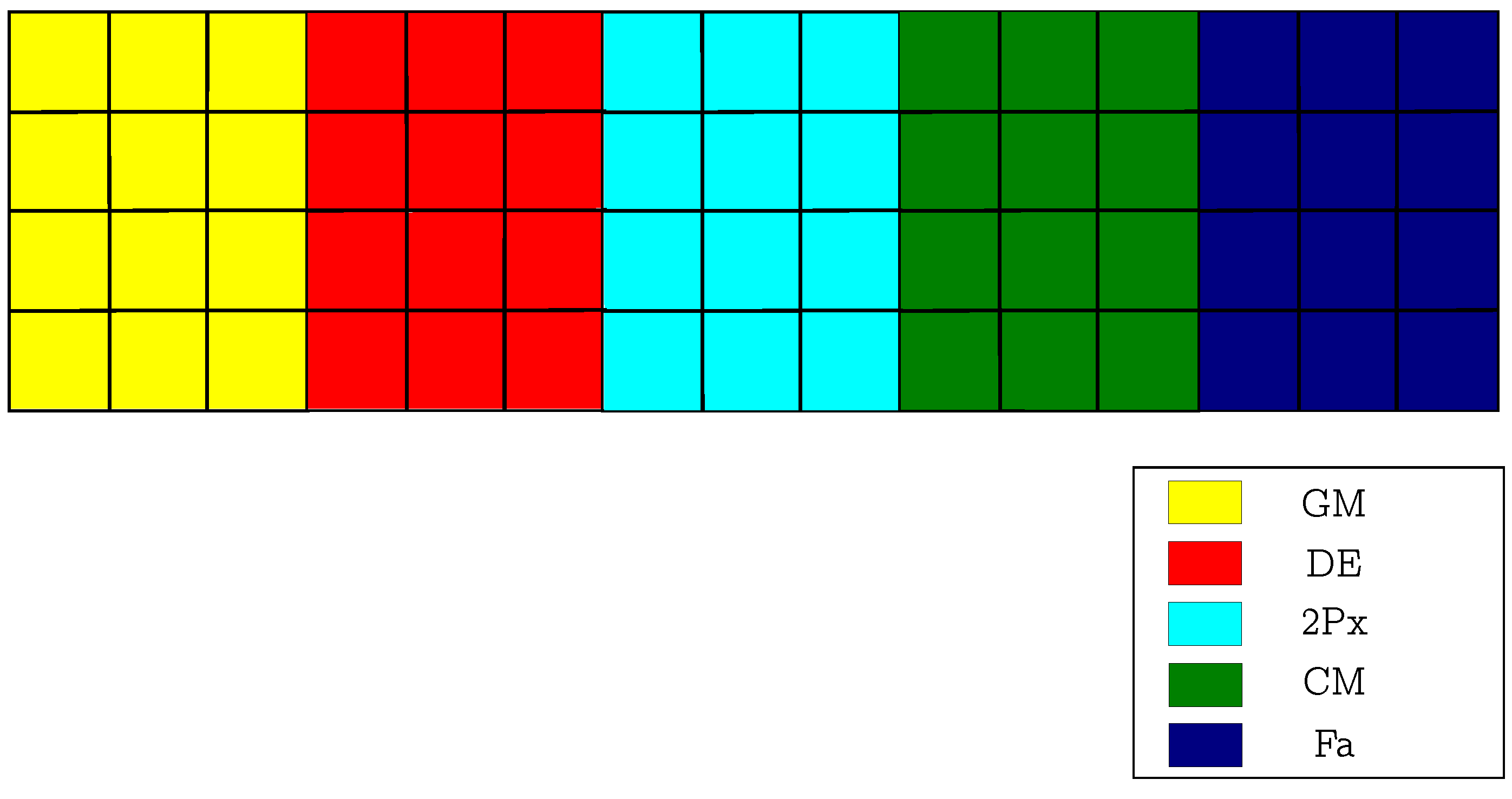
2.1. The CRO-SL: A Multi-Method-Ensemble Evolutionary Algorithm

The coral reef optimization algorithm with substrate layers (CRO-SL) [27,28] is a low-level ensemble for optimization [1], based on evolutionary computation. It was first proposed as an advanced version of a basic original algorithm, CRO [41]. We describe CRO-SL here but start by introducing the basic CRO approach first.

2.1.1. Basic CRO

The coral reef optimization algorithm (CRO) [29,41] is an evolutionary-type meta-heuristic—a class of hybrid between evolutionary algorithms [42] and simulated annealing [43]. CRO uses a model of a rectangular-shaped reef that is $M\times N$, ($\Lambda$), where the possible solutions to the problem at hand (corals) are set. Each space $\Lambda (i,j)$, where i and j are the space’s coordinates, can be empty or contain a coral ${\mathbf{x}}_k$. The algorithm evolves the solutions in the reef, as follows:

1.

Initialization: A fraction ${\rho }_0$ of the total reef capacity is occupied with randomly generated corals. The reef position that each coral occupies is also randomly selected.

2.

Evolution: Once the reef has been populated, the evolutionary process begins. This process is divided into five phases per generation:

(a)

Sexual reproduction: In this phase, new solutions (larvae set) are created from the ones belonging to the reef in order to compete for a place in the reef. Sexual reproduction can be performed in two ways: external and internal. A percentage ($F_b$) of the corals settled in the reef perform external reproduction (Broadcast spawning), and the rest of them $(1-F_b)$ reproduce themselves through internal sexual reproduction (brooding). These reproduction processes are performed as follows:

i.

Broadcast spawning: from the set of corals selected for external sexual reproduction ($F_b$), new solutions (larvae) are generated and released.

ii.

Brooding: each one of the remaining corals ($1-F_b$) produces a larva by means of a small perturbation and releases it.

(b)

Larvae setting: In this step, all the larvae produced by broadcast spawning or brooding try to find a spot in the reef to grow up. A reef position is randomly chosen, and the larva will settle in that spot in only one of the following scenarios:

i.

The spot is empty.

ii.

The larva has a better health function value (fitness) than the coral currently occupying that spot.

Each larva can try to settle in the reef a maximum of three times. If the larva has not been able to settle down in the reef after that number of attempts, it is discarded.

(c)

Asexual reproduction: In this phase (also called budding), a fraction $F_a$ of the corals with better fitness present in the reef duplicate themselves, and after a small number of mutations, are released. They will try to settle in the reef as in the previously described step.

(d)

Depredation: Finally, each coral belonging to the $F_{dep}$ worst fraction can be predated (erased from the reef) with a low probability, $P_d$.

This basic version of the algorithm works as an evolutionary-type approach, defined in exploitation, not in exploration, as the majority of algorithms do. This means that we can use any kind of search procedure in the CRO. In fact, the first algorithm in [41] uses a 2-point crossover operator to perform the broadcast spawning, but in other cases, alternative operators are considered, such as harmony search operators [44] or $\beta$-hillclimbing [45]. Note that this paves the way to defining an improved algorithm as a multi-method ensemble.

2.1.2. CRO with Substrate Layers (CRO-SL)

The CRO-SL algorithm [27,28] is a further evolution of the CRO approach towards a multi-method ensemble. It generally proceeds as the basic CRO, but with a significant difference: instead of having a single surface of $M\times N$, it considers several substrate layers (T) of approximately the same size in the reef (Figure 1). Each substrate, in turn, represents a particular evolution strategy or searching procedure. Thus, the CRO-SL is a multi-method ensemble algorithm [1], where several searching strategies are carried out within a single population.

Figure 1 shows a visual description of the CRO-SL procedure. This new approach adds a dimension to the reef $\Lambda$, so a reef’s position is now given by three coordinates $\Lambda (t,i,j)$, where t is the substrate index, and i and j have the same meanings as in basic CRO. In Figure 1, the third dimension is represented with colors. Thus, the evolutionary process is the same as in the basic CRO at a general level, but the reproduction phase is performed at the substrate level, so that a different search operator is applied depending on the substrate the solution is allocated. The brooding phase remains the same as the basic CRO, for all substrates. The produced larvae are released to a common reservoir, and then the larvae setting procedure is carried out as in the basic CRO, regardless of its original substrate.

2.2. Substrate Layers Defined in the CRO-SL

Very different search strategies can be defined in the CRO-SL as part of the multi-method approach, and they affect the performance of the ensemble. They are usually defined at the practitioner’s discretion. In related articles, different combinations of well-known meta-heuristics have been defined. In this case, we again tested regular combinations of previously-defined heuristics and meta-heuristics, depending on the problem at hand. Specifically, we have defined and applied the following substrates in the CRO-SL and its new variants: DE (different versions), the Firefly algorithm (Fa), classical two-point crossover (2Px), BLX-$\alpha$ crossover (BLX), Gaussian-based mutation (GM), and Cauchy-based mutation (CM).

• DE: The DE algorithm [15] is a stochastic population-based method specifically designed for global optimization problems [46]. In its more common form, DE maintains a population with $N_p$ individuals, where every individual within the population stands for a possible solution to the problem. Individuals are represented by a vector $X_{i,g}$, where $i=1,\dots ,N_p$ and g refers to the index of the generation. A normal DE cycle consists of three consecutive steps: mutation, crossover, and selection. We adapted the algorithm for the CRO-SL by considering only the mutation and crossover parts of the meta-heuristic. Thus, mutation is carried out to generate random perturbations on the population. For each individual, a mutant vector is generated. There are different approaches for DE mutation in the literature [15]. We describe here the procedure known as the “best mutation strategy” [47], which has been successfully applied in many optimization problems before. It attempts to mutate the best individual of the population, according to Equation (1), where $V_{i,g}$ denotes the mutated vector, i is the index of the vector, g stands for the generation index, $r_1,r_2\in 1,\dots ,N_p$ are randomly created integers, $X_{best,g}$ denotes the best solution in the population, and F is the scaling factor in the interval $[0,2]$. This mutation strategy uses the scaled difference between two randomly selected vectors to mutate the best individual in the population.

  $$V_{i,g}=X_{best,g}+F·(X_{r1,g}-X_{r2,g})$$

  (1)
  A crossover procedure is then applied between the mutated vector created in the mutation stage and an individual randomly chosen from the population. The new solutions created are called trial vectors and denoted by $T_{i,g}$ for individual i at generation g. Every parameter in the trial vector is decided following Equation (2), where j represents the index of every parameter in a vector, $CR$ is the probability of recombination, and $J_{rand}$ denotes a randomly selected integer within $(1,\dots ,N_p)$ to ensure that at least one parameter from the mutated vector enters the trial vector:

  $$T_{i,g}\left[j\right]=\left\{\begin{array}{cc}{V}_{i,g}\left[j\right]\hfill & \mathrm{if}rand[0,1]<CR\mathrm{or}j=j_{rand}\hfill \\ X_{i,g}\left[j\right]\hfill & \mathrm{otherwise}\hfill \end{array}\right.$$

  (2)
• Fa: The Fa is a kind of swarm intelligence algorithm based on the flashing patterns and behavior of fireflies in nature [48,49]. In this algorithm, the pattern movement of a firefly i attracted to another (brighter) firefly j is calculated as follows:

  $${\mathbf{x}}_i^{t+1}={\mathbf{x}}_i^t+{\beta }_0{e}^{-\gamma r_{ij}^2}({\mathbf{x}}_j^t-{\mathbf{x}}_i^t)+\alpha {ϵ}_i^t$$

  (3)

  where ${\beta }_0$ stands for the attractiveness at distance $r=0$. The specific Fa mutation implemented in the CRO-SL is a modified version of the algorithm known as the neighborhood attraction firefly algorithm (NaFa) [50]. It has been implemented as follows: When a coral (solution) in the reef belongs to the Fa substrate, it is updated following Equation (3). All the parameters of the equation are tuned during the CRO-SL evolution. The corals in the Fa substrate consider as swarm a neighborhood among all other corals in the reef (not only the Fa substrate). Thus, the corals in the Fa substrate are updated taking into account some solutions from other substrates, since all the corals in the reef share the same objective function.
• 2Px: Classical 2-point crossover. The crossover operator is the most classical exploration mechanism in genetic and evolutionary algorithms [42,51]. It consists of coupling individuals at random, choosing two points for the crossover, and interchanging the genetic material between both points. In the classical version of the CRO-SL, one individual to be crossed is from the 2Px substrate, whereas the couple can be chosen from any part of the reef.
• BLX: BLX-$\alpha$ crossover. This crossover operator [52] considers two real-encoded vectors, $x_1=(x_{11},\dots ,x_{n1})$ and $x_2=(x_{12},\dots ,x_{n2})$, and generates two offspring, $h^k=(h_1^k,\dots ,{\delta }_i^k,\dots ,h_n^k)$, $k=1,2$, where ${\delta }_i^k$ is a randomly (uniformly) chosen number from the interval $\left[x_{min}-I\alpha ,x_{max}+I\alpha \right]$, where $x_{max}=max(x_{i1},x_{i2})$, $x_{min}=min(x_{i1},x_{i2})$, and $I=x_{max}-x_{min}$.
• GM: Gaussian mutation with a $\sigma$ value linearly decreasing during the run, from $0.2·(A-B)$ to $0.02·(A-B)$, where $[B,A]$ is the domain search. Specifically, the Gaussian probability density function is:

  $$f_{G(0,{\sigma }^2)}\left(x\right)=\frac{1}{\sigma \sqrt{2\pi }}{e}^{-\frac{x^2}{2{\sigma }^2}}.$$
  The reason for adapting the value of $\sigma$ throughout the generations is to provide more mutations in the beginning of the optimization and fine tuning with smaller displacements nearing the end. The mutated larva is thus calculated as: $x_i^{\prime }=x_i+\delta N_i(0,1)$, where $N_i(0,1)$ is a random number following the Gaussian distribution.
• CM: Cauchy mutation. The one-dimensional Cauchy density function centered at the origin is defined by:

  $$f_t\left(x\right)=\frac{1}{\pi }\frac{t}{t^2+x^2}$$

  (4)

  where $t>0$ is a scale parameter [53]; in this case, $t=1$. Note that the Cauchy probability distribution looks like the Gaussian distribution, but it approaches the axis so slowly that an expectation does not exist. As a result, the variance of the Cauchy distribution is infinite [53]. In this case, the mutated larva is calculated as: $x_i^{\prime }=x_i+\eta \delta$, where $\eta$ stands for a variance and $\delta$ is a random number following the Cauchy distribution.

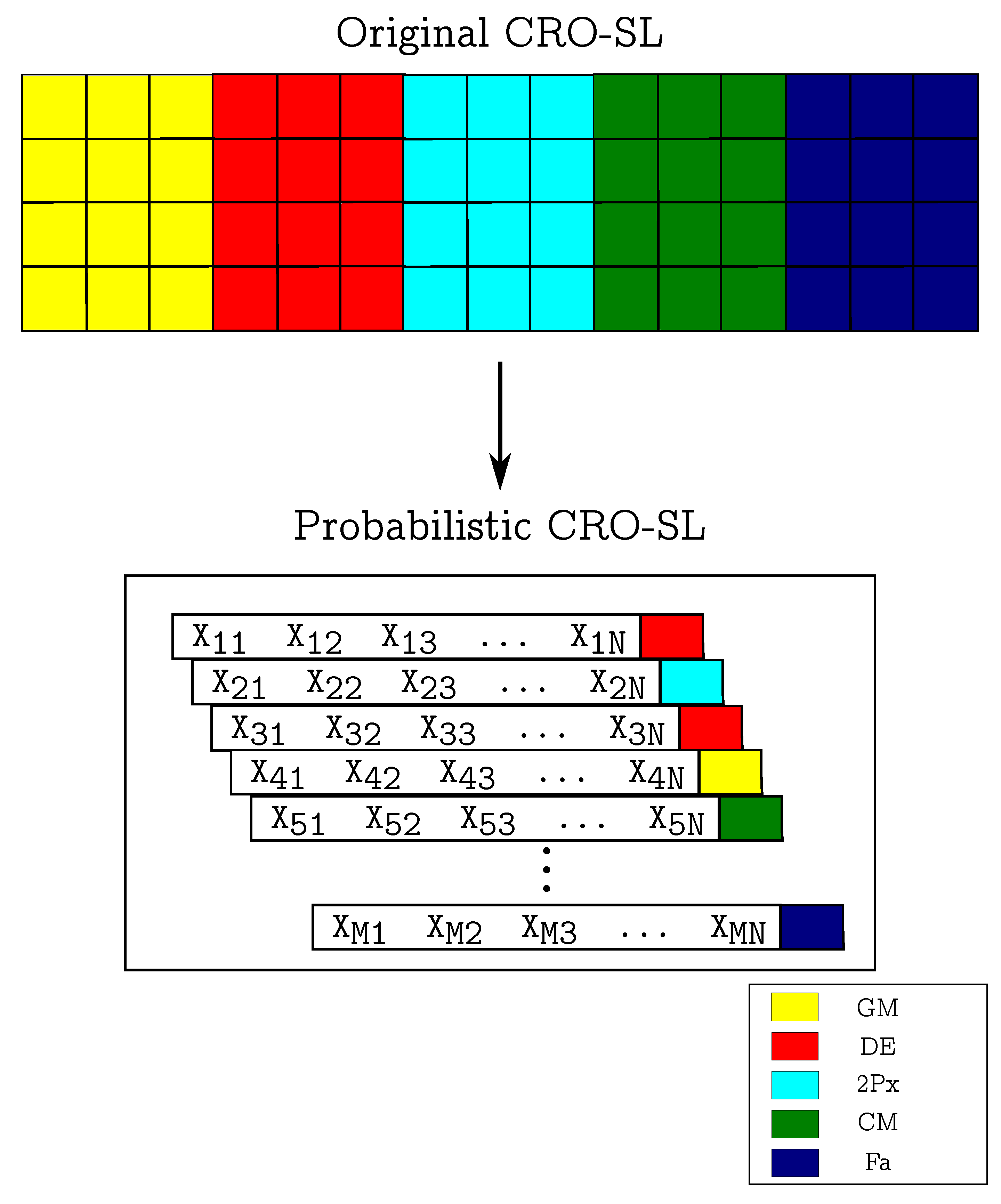
3. Proposed Probabilistic Dynamic Ensembles with the CRO-SL

In this section, we present the two newly proposed multi-method ensemble methods based on CRO-SL. Note that the main contribution of these new ensembles is the way that each search procedure is selected for offspring generation, in such a way that it only affects the broadcast spawning process, which was previously defined. In the original CRO-SL algorithm, each search procedure is assigned to a set of positions of the population (substrate). Thus, every individual settled on one of these positions will follow the same search method in every iteration. Now, in these new CRO-SL versions, the search procedures are chosen dynamically for each parent in each iteration of the run. This means that the search procedures are no longer tied to a set of positions, but a coral will produce the offspring in each iteration following one of the search procedures, which is randomly chosen. The main difference between both versions is whether the probabilities are fixed and maintained during the algorithm’s run or changed dynamically according to the search procedure’s performance.

3.1. Probabilistic CRO-SL Ensemble

The probabilistic CRO-SL ensemble (PCRO-SL) is constructed from using the original CRO-SL, by changing the substrate structure for a tag associated with each coral (solution) in the reef. Each tag t stands for the substrate index in this case. The main difference with the CRO-SL is that in each generation, the assignment of tags to corals is changed, so for a given coral, the search procedure changes in each generation according to a given probability distribution, usually a uniform one. Figure 2 shows an example of the PCRO-SL, comparing a reef in it with one in the original CRO-SL.

In essence, PCRO-SL lets the search methods be independent of the positions in the reef, which still has a size of $M\times N$. Now, the substrates are not defined by specific positions in the reef, but they will be formed by a set of individuals randomly distributed throughout the reef. The probability of using one search method or another for an individual in any iteration of the run is defined by Equation (5).

$$p_i=1/T$$

(5)

where $p_i$ stands for the probability that an individual belongs to substrate i and T stands for the number of search procedures (substrates) considered. Note that, in this case, the probabilities $p_i$ do not change during the run; however, the assignment of individuals to each substrate is carried out every generation. Algorithm 1 shows the pseudo-code of this PCRO-SL version.

Algorithm 1 Probabilistic CRO-SL.

Input: values of the algorithm parameters within the range, including the probabilities of each search method. Output: the fittest solution found for the problem at hand. Step 1: set the initial population and empty positions, and calculate their fitness values. Step 2: each individual can create new solutions in two ways: if  $F_b$  then     with a high probability $F_b$ it is generated offspring by the broadcast spawning process: in this version, one search method is randomly selected (with probability $p_i$, given by Equation (5)) among the candidates. else     with a low probability $(1-F_b)$ it is generated offspring by the brooding process. end if Step 3: perform the settlement of the offspring. Step 4: with probability $P_d$ the depredation process is carried out. Step 5: return the optimal solution if the stopping criterion is hold or go back to step 2 otherwise.

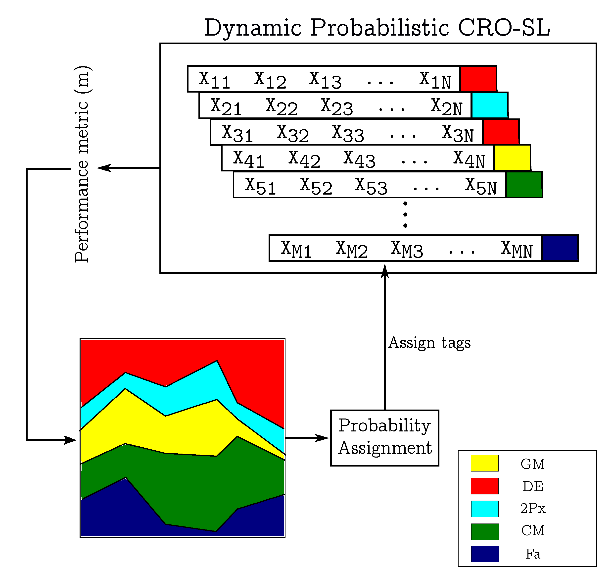
3.2. Dynamic Probabilistic CRO-SL Ensemble

The PCRO-SL ensemble method described above can be improved by including a dynamic procedure of method-probability assignment, in such a way that the most efficient methods have higher chances of being assigned than other search approaches, which have not been so good during the search. Note that there are different methods for carrying out this dynamical assignment. Specifically, we have evaluated three different ways of calculating the probability of the search method to be assigned to corals in the reef:

1.

Larval success rate metric. The first probability-assignment procedure depends on the rate of success of the larvae (new solutions) produced by the corals in each substrate. In other words, during the larvae setting phase, we keep track of the substrate (search method) from which each larva was produced, and we note the number of them that were successful in being inserting into the reef. The probability of each searching method in the next step is obtained as the rate of successes of the total number of generated larvae.

2.

Raw fitness metric. The second probability-assignment procedure uses the fitness of the generated solutions; i.e., it considers the quality of individual solutions to obtain a metric for each substrate. In other words, if the operator applied generates good solutions, it will have a higher probability of being assigned to an individual in the next step. Note that there are different ways of implementing this metric: for example, we can take the average of the fitness levels of all the larvae produced, the best fitness across all of them, the worst one, etc.

3.

Improvement of fitness. The last procedure for assigning the methods probabilities is a differential approach, based on the difference from the best fitness level obtained in the previous generation. It works very similarly to the previous strategy, giving higher values to those substrates that generated solutions with better fitness. This method also allows some variants, so we can take the average of the difference, the best value, or the worst value to assign the probability of the method being used in the next step.

Once each substrate has been evaluated, the probability distribution can be calculated from the metric considered, to finally assign the probability for a given substrate in the next generation. To do this, the softmax function is used, so the probability assigned to one of the T substrates i with a metric $m_i$ can be calculated as follows:

$$p_i=\frac{e^{m_i/\tau }}{{\sum }_{j=0}^S{e}^{m_j/\tau }}$$

(6)

where the parameter $\tau$ gives a way of “amplifying” the probabilities, i.e., making similar changes in the metric of each substrate giving high probabilities for low values of $\tau$. Note that this process of new probability assignment is carried out after a number of generations, $\mathcal{T}$—enough generations that we can evaluate the performances of the different search methods in the problem at hand. Figure 3 shows an outline of the DPCRO-SL ensemble.

To ensure that the space of operators is effectively explored, a probability threshold is set, $\epsilon$, so that all substrates have at least a probability $\epsilon$ of being assigned to an individual. This probability can be very small but must be enough to ensure that the operator will eventually be chosen. Algorithm 2 shows the pseudo-code of the DPCRO-SL version.

Algorithm 2 Dynamic probabilistic CRO-SL.

Input: values of the algorithm parameters within the range. Output: the fittest solution found for the problem at hand. Step 1: set the initial population and empty positions, and calculate their fitness values. Step 2: each individual can create new solutions in two ways: if  $F_b$  then     with a high probability $F_b$ it is generated offspring by the broadcast spawning process: in this version, one search method is randomly selected (with probability $p_i$ given by Equation (6)) among the candidates. else     with a low probability $(1-F_b)$ it is generated offspring by the brooding process. end if Step 3: perform the settlement of the offspring. Step 4: calculate the success ratio of each search method and update the probabilities following Equation (6). Step 5: with probability $P_d$ the predation process is carried out. Step 6: return the optimal solution if the stopping condition is met, go back to step 2 otherwise.

4. Experimental Results

The evaluation of the proposed CRO-SL variants was carried out in different benchmark functions and also in a real application of wind-turbine layout.

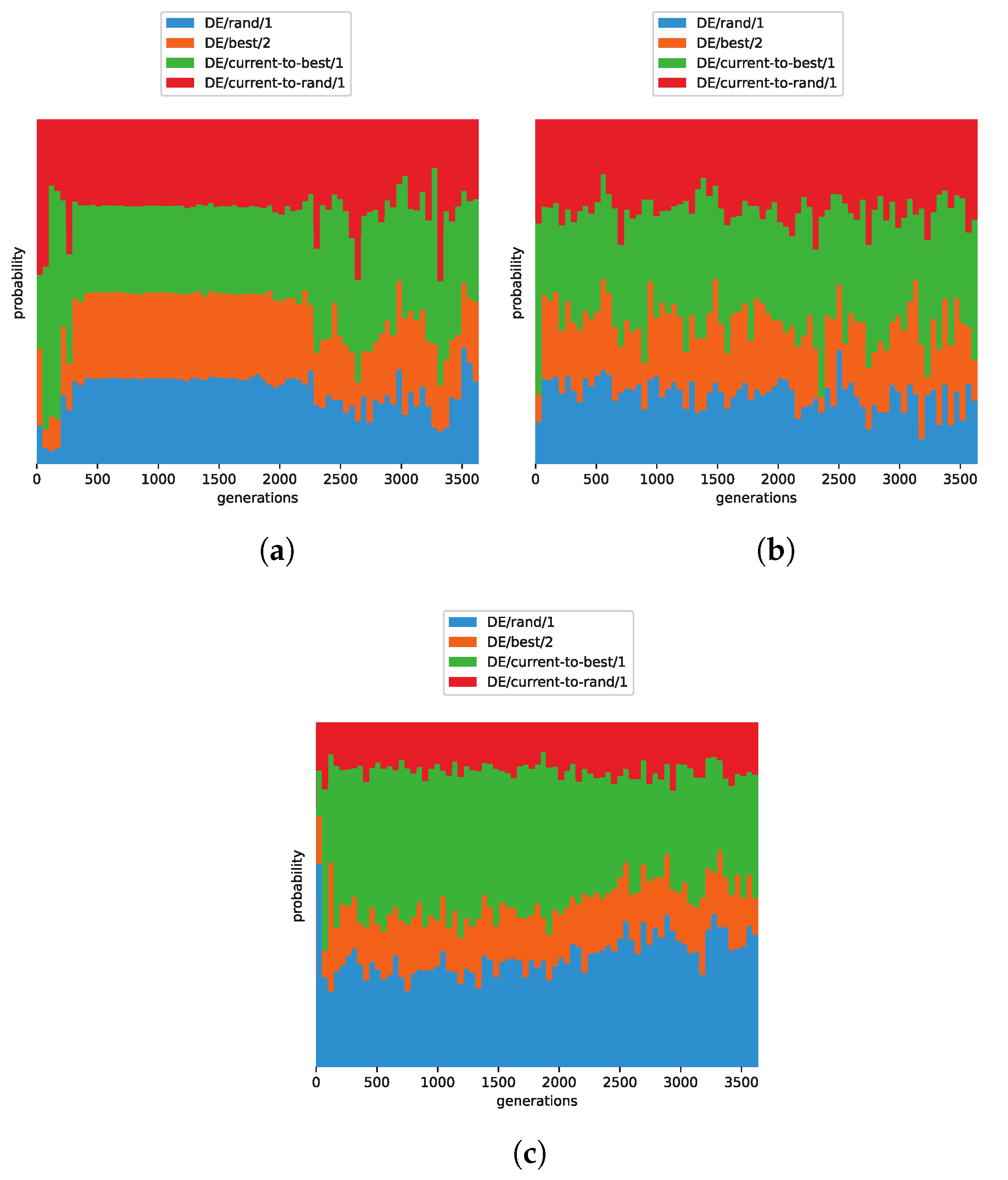
4.1. Comparison in Benchmark Functions

In this section, we compare the performances of PCRO-SL and DPCRO-SL with those of CRO-SL and other state-of-the-art algorithms on different benchmark functions, to evaluate the goodness of the two newly proposed probabilistic CRO-SL ensembles. The definitions of the 25 benchmark functions considered can be found in the Appendix A. In a first set of experiments, both PCRO-SL and DPCRO-SL were evaluated considering the combination of four DE approaches in the ensemble as search methods. The reason for defining a DE-based ensemble for the experiments with benchmark functions is that DE-based approaches have obtained excellent results in the past in these kinds of problems, such as the linear population size reduction success-history based adaptive differential evolution (LSHADE) approach [19,26]. For each of the 25 benchmark functions 10 to $3\times {10}^5$ evaluations of the objective functions were considered (the latter being the limit), and the best, average, and standard deviation were obtained for the 10 executions carried out.

The defined DE-based CRO-SL is a version of the algorithm in which the operators to be used in each substrate are restricted to a variant of the cross operation in the DE (differential evolution) algorithm (see Section 2.2). To define a DE variant, the notation is usually “DE/a/b”, where a determines which vectors are going to selected and b determines how many differences are going to be calculated. Hence, the variant DE/rand/2 will take 5 vectors at random from the population—$X_{r1,g},X_{r2,g},X_{r3,g},X_{r4,g},X_{r5,g}$—and will calculate the vector V:

$$V_{i,g}=X_{r1,g}+F·(X_{r2,g}-X_{r3,g})+F·(X_{r4,g}-X_{r5,g})$$

which will be crossed with the individual chosen in the same way as in the DE algorithm.

In these experiments on benchmark functions, we first used the following DE variants:

1.

DE/best/1

$$V_{i,g}=X_{best,g}+F·(X_{r1,g}-X_{r2,g})$$

2.

DE/best/2

$$V_{i,g}=X_{best,g}+F·(X_{r1,g}-X_{r2,g})+F·(X_{r3,g}-X_{r4,g})$$

3.

DE/current-to-best/1

$$V_{i,g}=X_{i,g}+U·(X_{best,g}-X_{i,g})+F·(X_{r1,g}-X_{r2,g})$$

4.

DE/current-to-pbest/1

$$V_{i,g}=X_{i,g}+F·(X_{pbest,g}-X_{i,g})+F·(X_{r1,g}-X_{r2,g})$$

where U is a random value following a uniform probability distribution between 0 and 1, $X_{best,g}$ is the individual with the best fitness in generation g, $X_{pbest,g}$ is a solution picked at random from the $p\%$ best ones in the generation, $X_{i,g}$ is the individual chosen to be crossed with, and $X_{rn,g}$ is an individual chosen at random from the population.

Before further testing the performances of the proposed ensembles, the different methods of probability assignment proposed were evaluated. Figure 4a–c compare different methods of probability assignment in the DPCRO-SL (raw fitness assignment, fitness improvement, and larval success rate, as described in Section 3.2). Note that the probability is depicted in a relative plot fashion, so a color’s thickness represents the probability of the given search method’s assignment. This is an example for the optimization of the Rosenbrock function (F5) with a limit of $3·{10}^5$ evaluations of the function. The probability that is assigned to each operator in each generation of the algorithm is shown in the figure. It is possible to see differences in the probability-assignment process. After some experimental tests, the best results were obtained with the raw fitness probability-assignment process. The rest of the results in these benchmark functions were therefore obtained with this probability-assignment method.

Table 1. Comparison among different CRO-SL ensemble variants (CRO-SL, PCRO-SL and DPCRO-SL) with 4 DE-based substrates. We indicate the best mean fitness for each CRO variant in bold text.

Function	DPCRO-SL			PCRO-SL			CRO-SL
#	Best	Mean	Std	Best	Mean	Std	Best	Mean	Std
F1	$4.16\times {10}^{-78}$	$\mathbf{3.20}\times {\mathbf{10}}^{-\mathbf{76}}$	$4.99\times {10}^{-76}$	$7.60\times {10}^{-62}$	$1.20\times {10}^{-60}$	$1.95\times {10}^{-60}$	$1.91\times {10}^{-68}$	$8.07\times {10}^{-58}$	$1.91\times {10}^{-57}$
F2	$2.63\times {10}^{-77}$	$\mathbf{6.86}\times {\mathbf{10}}^{-\mathbf{75}}$	$1.29\times {10}^{-74}$	$2.98\times {10}^{-61}$	$7.20\times {10}^{-60}$	$9.00\times {10}^{-60}$	$5.07\times {10}^{-63}$	$1.19\times {10}^{-56}$	$3.57\times {10}^{-56}$
F3	$1.75\times {10}^{-72}$	$\mathbf{1.42}\times {\mathbf{10}}^{-\mathbf{69}}$	$3.12\times {10}^{-69}$	$1.83\times {10}^{-55}$	$1.05\times {10}^{-54}$	$1.45\times {10}^{-54}$	$3.22\times {10}^{-61}$	$2.26\times {10}^{-48}$	$6.03\times {10}^{-48}$
F4	$1.63\times {10}^{-81}$	$\mathbf{1.42}\times {\mathbf{10}}^{-\mathbf{78}}$	$2.25\times {10}^{-78}$	$4.00\times {10}^{-64}$	$3.43\times {10}^{-63}$	$3.41\times {10}^{-63}$	$1.68\times {10}^{-68}$	$5.00\times {10}^{-54}$	$1.50\times {10}^{-53}$
F5	$2.34\times {10}^{-16}$	$\mathbf{1.49}\times {\mathbf{10}}^{-\mathbf{10}}$	$4.44\times {10}^{-10}$	$8.98\times {10}^{-13}$	$3.99\times {10}^{-1}$	$1.20$	$1.19\times {10}^{-15}$	$6.63\times {10}^{-8}$	$1.33\times {10}^{-7}$
F6	$3.55\times {10}^{-15}$	$\mathbf{3.55}\times {\mathbf{10}}^{-\mathbf{15}}$	$0.00$	$3.55\times {10}^{-15}$	$\mathbf{3.55}\times {\mathbf{10}}^{-\mathbf{15}}$	$0.00$	$3.55\times {10}^{-15}$	$\mathbf{3.55}\times {\mathbf{10}}^{-\mathbf{15}}$	$0.00$
F7	$-6.00\times {10}^1$	$-\mathbf{6.00}\times {\mathbf{10}}^{\mathbf{1}}$	$2.66\times {10}^{-14}$	$-6.00\times {10}^1$	$-\mathbf{6.00}\times {\mathbf{10}}^{\mathbf{1}}$	$3.03\times {10}^{-14}$	$-6.00\times {10}^1$	$-\mathbf{6.00}\times {\mathbf{10}}^{\mathbf{1}}$	$3.87\times {10}^{-14}$
F8	$0.00$	$2.71\times {10}^{-3}$	$4.33\times {10}^{-3}$	$0.00$	$\mathbf{7.40}\times {\mathbf{10}}^{-\mathbf{4}}$	$2.22\times {10}^{-3}$	$0.00$	$1.97\times {10}^{-3}$	$4.09\times {10}^{-3}$
F9	$1.39\times {10}^1$	$5.73\times {10}^1$	$5.57\times {10}^1$	$1.79\times {10}^1$	$\mathbf{3.24}\times {\mathbf{10}}^{\mathbf{1}}$	$2.54\times {10}^1$	$1.49\times {10}^1$	$4.99\times {10}^1$	$5.48\times {10}^1$
F10	$0.00$	$\mathbf{0.00}$	$0.00$	$0.00$	$\mathbf{0.00}$	$0.00$	$0.00$	$\mathbf{0.00}$	$0.00$
F11	$0.00$	$\mathbf{0.00}$	$0.00$	$0.00$	$\mathbf{0.00}$	$0.00$	$0.00$	$\mathbf{0.00}$	$0.00$
F12	$-4.06\times {10}^2$	$-\mathbf{4.06}\times {\mathbf{10}}^{\mathbf{2}}$	$5.68\times {10}^{-14}$	$-4.06\times {10}^2$	$-\mathbf{4.06}\times {\mathbf{10}}^{\mathbf{2}}$	$5.68\times {10}^{-14}$	$-4.06\times {10}^2$	$-\mathbf{4.06}\times {\mathbf{10}}^{\mathbf{2}}$	$5.68\times {10}^{-14}$
F13	$4.94\times {10}^{-1}$	$\mathbf{5.18}\times {\mathbf{10}}^{-\mathbf{1}}$	$1.37\times {10}^{-2}$	$4.92\times {10}^{-1}$	$\mathbf{5.18}\times {\mathbf{10}}^{-\mathbf{1}}$	$1.45\times {10}^{-2}$	$4.98\times {10}^{-1}$	$5.20\times {10}^{-1}$	$1.25\times {10}^{-2}$
F14	$2.20\times {10}^8$	$\mathbf{2.20}\times {\mathbf{10}}^{\mathbf{8}}$	$1.65\times {10}^{-1}$	$2.20\times {10}^8$	$\mathbf{2.20}\times {\mathbf{10}}^{\mathbf{8}}$	$2.18\times {10}^{-1}$	$2.20\times {10}^8$	$\mathbf{2.20}\times {\mathbf{10}}^{\mathbf{8}}$	$4.99\times {10}^{-1}$
F15	$3.47\times {10}^{-1}$	$\mathbf{3.47}\times {\mathbf{10}}^{-\mathbf{1}}$	$1.98\times {10}^{-8}$	$3.47\times {10}^{-1}$	$3.47\times {10}^{-1}$	$3.62\times {10}^{-8}$	$3.47\times {10}^{-1}$	$3.47\times {10}^{-1}$	$2.33\times {10}^{-8}$
F16	$5.95\times {10}^{-4}$	$2.04\times {10}^{-2}$	$1.70\times {10}^{-2}$	$2.58\times {10}^{-5}$	$1.90\times {10}^{-2}$	$1.79\times {10}^{-2}$	$3.23\times {10}^{-3}$	$\mathbf{1.72}\times {\mathbf{10}}^{-\mathbf{2}}$	$1.44\times {10}^{-2}$
F17	$1.17\times {10}^1$	$1.21\times {10}^1$	$6.01\times {10}^{-1}$	$1.17\times {10}^1$	$1.26\times {10}^1$	$7.13\times {10}^{-1}$	$1.17\times {10}^1$	$\mathbf{1.20}\times {\mathbf{10}}^{\mathbf{1}}$	$5.77\times {10}^{-1}$
F18	$1.18\times {10}^{-3}$	$1.20\times {10}^{-3}$	$2.87\times {10}^{-5}$	$1.18\times {10}^{-3}$	$5.15\times {10}^{-3}$	$7.92\times {10}^{-3}$	$1.00\times {10}^{-4}$	$\mathbf{1.09}\times {\mathbf{10}}^{-\mathbf{3}}$	$3.29\times {10}^{-4}$
F19	$-1.00$	$-1.53\times {10}^{-1}$	$2.85\times {10}^{-1}$	$-1.00$	$-\mathbf{2.52}\times {\mathbf{10}}^{-\mathbf{1}}$	$3.75\times {10}^{-1}$	$-1.00$	$-1.76\times {10}^{-1}$	$2.75\times {10}^{-1}$
F20	$3.72\times {10}^9$	$\mathbf{3.72}\times {\mathbf{10}}^{\mathbf{9}}$	$0.00$	$3.72\times {10}^9$	$\mathbf{3.72}\times {\mathbf{10}}^{\mathbf{9}}$	$0.00$	$3.72\times {10}^9$	$\mathbf{3.72}\times {\mathbf{10}}^{\mathbf{9}}$	$0.00$
F21	$-4.58\times {10}^1$	$-\mathbf{4.58}\times {\mathbf{10}}^{\mathbf{1}}$	$6.74\times {10}^{-15}$	$-4.58\times {10}^1$	$-\mathbf{4.58}\times {\mathbf{10}}^{\mathbf{1}}$	$2.25\times {10}^{-15}$	$-4.58\times {10}^1$	$-\mathbf{4.58}\times {\mathbf{10}}^{\mathbf{1}}$	$7.11\times {10}^{-15}$
F22	$0.00$	$1.94\times {10}^{-3}$	$3.89\times {10}^{-3}$	$0.00$	$2.91\times {10}^{-3}$	$4.45\times {10}^{-3}$	$0.00$	$\mathbf{9.72}\times {\mathbf{10}}^{-\mathbf{4}}$	$2.91\times {10}^{-3}$
F23	$-3.31$	$-\mathbf{3.24}$	$8.12\times {10}^{-2}$	$-3.31$	$-3.28$	$7.33\times {10}^{-2}$	$-3.31$	$-3.25$	$8.31\times {10}^{-2}$
F24	$-6.13$	$-\mathbf{6.13}$	$0.00$	$-6.13$	$-\mathbf{6.13}$	$0.00$	$-6.13$	$-\mathbf{6.13}$	$0.00$
F25	$0.00$	$\mathbf{3.00}\times {\mathbf{10}}^{-\mathbf{3}}$	$5.98\times {10}^{-3}$	$0.00$	$6.25\times {10}^{-3}$	$7.15\times {10}^{-3}$	$0.00$	$\mathbf{3.00}\times {\mathbf{10}}^{-\mathbf{3}}$	$5.98\times {10}^{-3}$

We indicate in bold text the best mean fitness for each algorithm.

shows the results obtained in the optimization of bechmark functions with the different CRO-SL approaches proposed, and the original one. As can be seen, PCRO-SL showed better performance than the classic CRO-SL in general. However, it is the DPCRO-SL approach which showed the best results of all CRO-SL versions, leading to very significant overall improvement in performance for all test functions. These results indicate that the DPCRO-SL performs more efficient management of the search resources in the ensemble, by means of modifying the probability of each search procedure as the algorithms evolve. However, this improvement is less noticeable from the 16th function onward. CRO-SL obtained a better mean for the fitness values. Note that this set of functions is different from the rest, since they have lower dimensionality, most of them having as an input a 2-dimensional vector, which could imply that the DPCRO-SL method is better suited for higher dimensional problems.

Further experiments were performed by carrying out a comparison with two existing meta-heuristic approaches that obtained excellent performances in previous works. Specifically, DPCRO-SL, a version of the PSO algorithm [54], and the LSHADE algorithm [26] were tested.

Table 2. Comparison of the DPCRO-SL ensemble with PSO [54] and LSHADE [26]. We indicate the best mean fitness for each algorithm in bold text.

Function	DPCRO-SL			PSO			LSHADE
#	Best	Mean	Std	Best	Mean	Std	Best	Mean	Std
F1	$4.16\times {10}^{-78}$	$\mathbf{3.20}\times {\mathbf{10}}^{-\mathbf{76}}$	$4.99\times {10}^{-76}$	$4.98\times {10}^{-33}$	$5.98\times {10}^{-31}$	$9.51\times {10}^{-31}$	$1.21\times {10}^{-79}$	$1.90\times {10}^{-73}$	$5.70\times {10}^{-73}$
F2	$2.63\times {10}^{-77}$	$\mathbf{6.86}\times {\mathbf{10}}^{-\mathbf{75}}$	$1.29\times {10}^{-74}$	$2.48\times {10}^4$	$1.72\times {10}^5$	$9.93\times {10}^4$	$4.14\times {10}^{-73}$	$1.60\times {10}^{-67}$	$4.56\times {10}^{-67}$
F3	$1.75\times {10}^{-72}$	$\mathbf{1.42}\times {\mathbf{10}}^{-\mathbf{69}}$	$3.12\times {10}^{-69}$	$2.24\times {10}^{-25}$	$8.00\times {10}^3$	$4.00\times {10}^3$	$2.05\times {10}^{-72}$	$3.89\times {10}^{-66}$	$1.04\times {10}^{-65}$
F4	$1.63\times {10}^{-81}$	$\mathbf{1.42}\times {\mathbf{10}}^{-\mathbf{78}}$	$2.25\times {10}^{-78}$	$5.27\times {10}^{-33}$	$6.29\times {10}^1$	$4.86\times {10}^1$	$8.53\times {10}^{-77}$	$3.61\times {10}^{-73}$	$6.33\times {10}^{-73}$
F5	$2.34\times {10}^{-16}$	$\mathbf{1.49}\times {\mathbf{10}}^{-\mathbf{10}}$	$4.44\times {10}^{-10}$	$1.25\times {10}^{-1}$	$2.02\times {10}^5$	$3.99\times {10}^5$	$6.13\times {10}^{-3}$	$8.84\times {10}^{-1}$	$9.16\times {10}^{-1}$
F6	$3.55\times {10}^{-15}$	$\mathbf{3.55}\times {\mathbf{10}}^{-\mathbf{15}}$	$0.00$	$7.11\times {10}^{-15}$	$1.21\times {10}^{-14}$	$3.26\times {10}^{-15}$	$3.55\times {10}^{-15}$	$3.91\times {10}^{-15}$	$1.07\times {10}^{-15}$
F7	$-6.00\times {10}^1$	$-\mathbf{6.00}\times {\mathbf{10}}^{\mathbf{1}}$	$2.66\times {10}^{-14}$	$-6.00\times {10}^1$	$-\mathbf{6.00}\times {\mathbf{10}}^{\mathbf{1}}$	$2.59\times {10}^{-14}$	$-6.00\times {10}^1$	$-\mathbf{6.00}\times {\mathbf{10}}^{\mathbf{1}}$	$0.00$
F8	$0.00$	$2.71\times {10}^{-3}$	$4.33\times {10}^{-3}$	$0.00$	$1.28\times {10}^{-2}$	$1.06\times {10}^{-2}$	$0.00$	$\mathbf{0.00}$	$0.00$
F9	$1.39\times {10}^1$	$5.73\times {10}^1$	$5.57\times {10}^1$	$6.77\times {10}^1$	$1.35\times {10}^2$	$4.08\times {10}^1$	$1.35\times {10}^{-6}$	$\mathbf{4.76}\times {\mathbf{10}}^{-\mathbf{5}}$	$1.10\times {10}^{-4}$
F10	$0.00$	$\mathbf{0.00}$	$0.00$	$0.00$	$2.21\times {10}^2$	$2.45\times {10}^2$	$0.00$	$\mathbf{0.00}$	$0.00$
F11	$0.00$	$\mathbf{0.00}$	$0.00$	$0.00$	$\mathbf{0.00}$	$0.00$	$0.00$	$\mathbf{0.00}$	$0.00$
F12	$-4.06\times {10}^2$	$-4.06\times {10}^2$	$5.68\times {10}^{-14}$	$-4.06\times {10}^2$	$-4.06\times {10}^2$	$5.68\times {10}^{-14}$	$-2.04\times {10}^3$	$-\mathbf{2.04}\times {\mathbf{10}}^{\mathbf{3}}$	$2.27\times {10}^{-13}$
F13	$4.94\times {10}^{-1}$	$5.18\times {10}^{-1}$	$1.37\times {10}^{-2}$	$4.90\times {10}^{-1}$	$4.93\times {10}^{-1}$	$2.08\times {10}^{-3}$	$4.96\times {10}^{-1}$	$\mathbf{5.03}\times {\mathbf{10}}^{-\mathbf{1}}$	$3.58\times {10}^{-3}$
F14	$2.20\times {10}^8$	$\mathbf{2.20}\times {\mathbf{10}}^{\mathbf{8}}$	$1.65\times {10}^{-1}$	$2.20\times {10}^8$	$4.56\times {10}^8$	$2.88\times {10}^8$	$2.20\times {10}^8$	$\mathbf{2.20}\times {\mathbf{10}}^{\mathbf{8}}$	$2.68\times {10}^{-1}$
F15	$3.47\times {10}^{-1}$	$\mathbf{3.47}\times {\mathbf{10}}^{-\mathbf{1}}$	$1.98\times {10}^{-8}$	$7.40\times {10}^{-1}$	$7.44\times {10}^{-1}$	$2.60\times {10}^{-3}$	$4.73\times {10}^{-1}$	$4.75\times {10}^{-1}$	$5.65\times {10}^{-3}$
F16	$5.95\times {10}^{-4}$	$\mathbf{2.04}\times {\mathbf{10}}^{-\mathbf{2}}$	$1.70\times {10}^{-2}$	$4.62\times {10}^{-3}$	$3.10\times {10}^{-2}$	$1.52\times {10}^{-2}$	$2.29\times {10}^2$	$2.29\times {10}^2$	$2.84\times {10}^{-14}$
F17	$1.17\times {10}^1$	$\mathbf{1.21}\times {\mathbf{10}}^{\mathbf{1}}$	$6.01\times {10}^{-1}$	$1.18\times {10}^1$	$1.40\times {10}^1$	$1.52$	$3.44\times {10}^2$	$3.44\times {10}^2$	$0.00$
F18	$1.18\times {10}^{-3}$	$\mathbf{1.20}\times {\mathbf{10}}^{-\mathbf{3}}$	$2.87\times {10}^{-5}$	$1.00\times {10}^{-4}$	$1.24\times {10}^{-2}$	$1.73\times {10}^{-2}$	$1.24$	$1.24$	$2.22\times {10}^{-16}$
F19	$-1.00$	$-\mathbf{1.53}\times {\mathbf{10}}^{-\mathbf{1}}$	$2.85\times {10}^{-1}$	$-1.00$	$-1.41\times {10}^{-1}$	$2.89\times {10}^{-1}$	$-8.04\times {10}^{-5}$	$-8.04\times {10}^{-5}$	$0.00$
F20	$3.72\times {10}^9$	$\mathbf{3.72}\times {\mathbf{10}}^{\mathbf{9}}$	$0.00$	$3.72\times {10}^9$	$\mathbf{3.72}\times {\mathbf{10}}^{\mathbf{9}}$	$0.00$	$3.89\times {10}^9$	$3.89\times {10}^9$	$0.00$
F21	$-4.58\times {10}^1$	$-\mathbf{4.58}\times {\mathbf{10}}^{\mathbf{1}}$	$6.74\times {10}^{-15}$	$-4.58\times {10}^1$	$-\mathbf{4.58}\times {\mathbf{10}}^{\mathbf{1}}$	$5.94\times {10}^{-15}$	$5.16\times {10}^2$	$5.16\times {10}^2$	$0.00$
F22	$0.00$	$\mathbf{1.94}\times {\mathbf{10}}^{-\mathbf{3}}$	$3.89\times {10}^{-3}$	$9.72\times {10}^{-3}$	$9.72\times {10}^{-3}$	$0.00$	$4.99\times {10}^{-1}$	$4.99\times {10}^{-1}$	$0.00$
F23	$-3.31$	$-3.24$	$8.12\times {10}^{-2}$	$-3.31$	$-\mathbf{3.05}$	$2.57\times {10}^{-1}$	$5.03\times {10}^1$	$5.03\times {10}^1$	$0.00$
F24	$-6.13$	$-\mathbf{6.13}$	$0.00$	$-6.13$	$-\mathbf{6.13}$	$0.00$	$0.00$	$0.00$	$0.00$
F25	$0.00$	$\mathbf{3.00}\times {\mathbf{10}}^{-\mathbf{3}}$	$5.98\times {10}^{-3}$	$2.60\times {10}^{-3}$	$7.99\times {10}^{-2}$	$1.10\times {10}^{-1}$	$5.19\times {10}^1$	$5.19\times {10}^1$	$0.00$

shows the results obtained in this comparison. It is shown that DPCRO-SL is able to obtain similar (in some cases better) performances to the PSO and LSHADE algorithms. In the most difficult benchmark functions, the differences were indeed significant. It is important to note that from function 16 onward, there was a significant performance drop by the LSHADE algorithm. This can be explained by the fact that these benchmark functions have one less dimension, and since the LSHADE approach uses a crossing procedure, the diversity obtained while running is reduced, and it is not able to successfully explore the whole space of possible solutions.

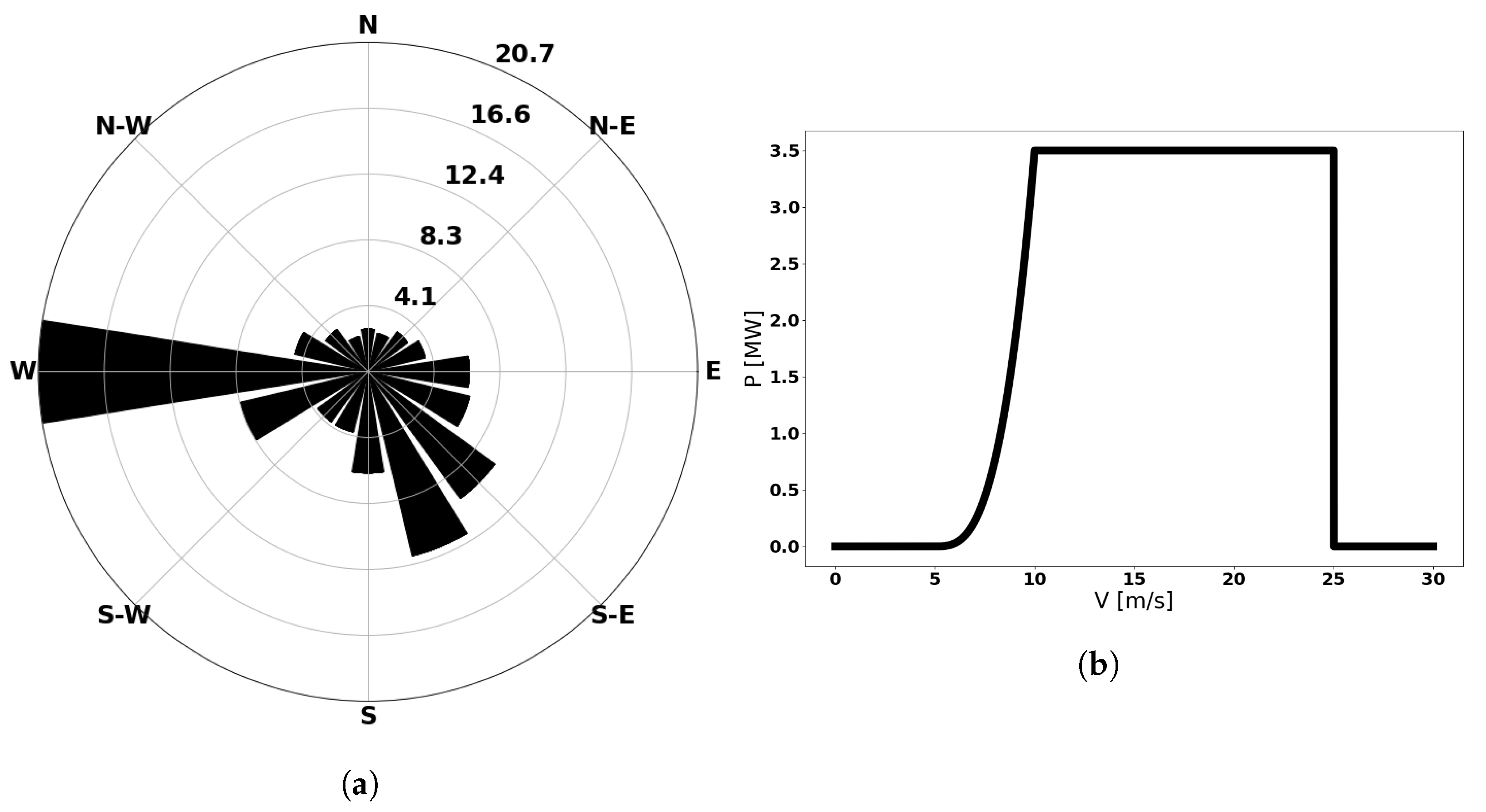
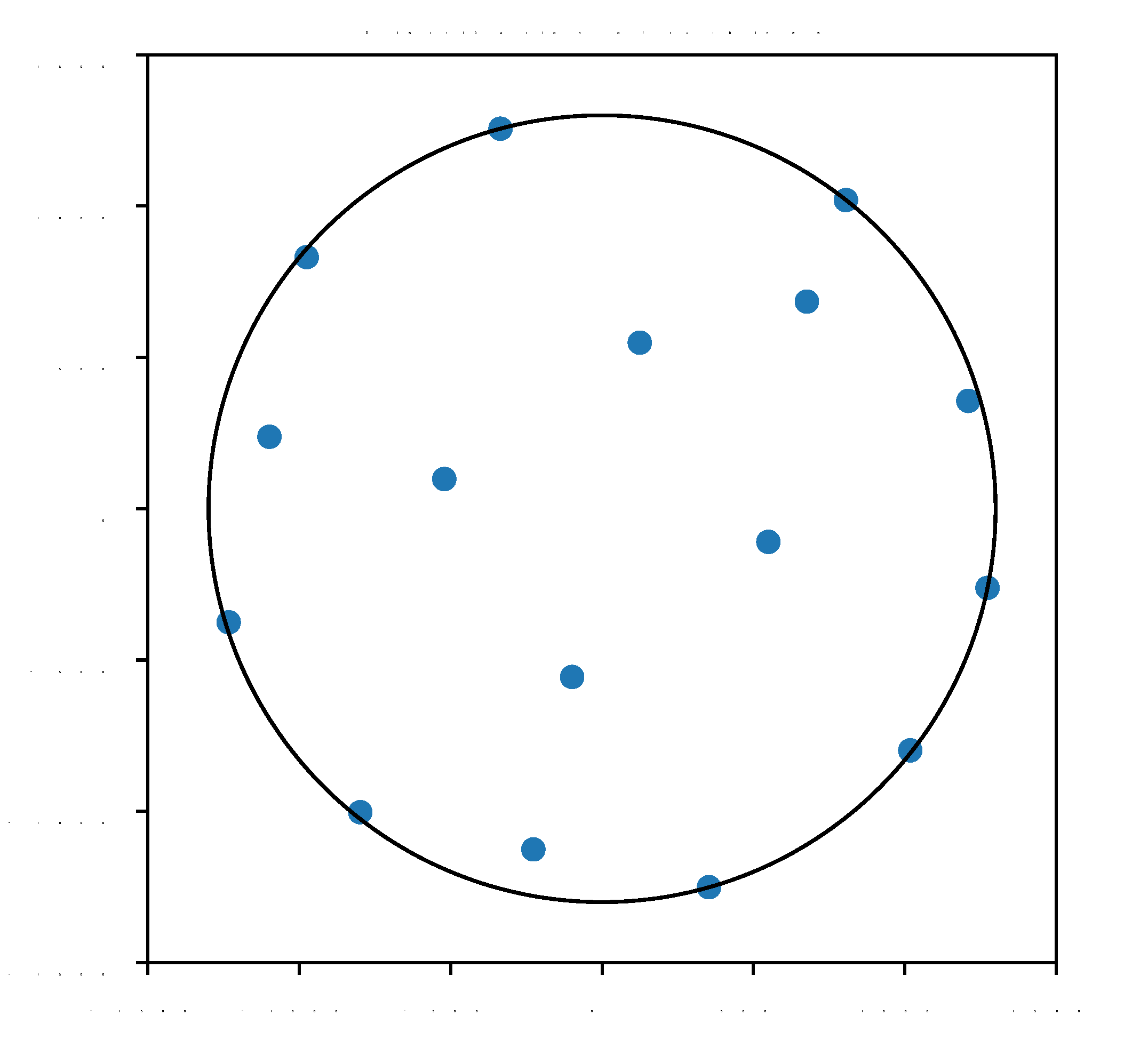
4.2. Comparison in a Real Problem—Wind-Turbine Assignment

To further test the performance of the proposed approach, DPCRO-SL, a case study of wind-turbine assignment has been addressed. The challenge is described in [55]. This challenge was proposed by the National Renewable Energy Lab (NREL) in the US, together with IEA (International Energy Agency) Wind Task 37, as a case competition in 2019. A circular symmetry wind farm is considered in this problem, on flat and level terrain. The wind turbines’ $(x,y)$ locations are restricted to be on or within the boundary radius of the wind farm. A separation constraint between turbines is also taken into account (a minimum distance of two rotor diameters between turbines is considered).

The wind characteristics considered for this challenge are specified in [55] and also described in [32]. Briefly, the wind distribution frequency and wind speed are the same for all wind-farm scenarios. Free-stream wind velocity is constant in all wind directions, fixed to $9.8$ m/s, for all days. The challenge considers a wind rose (Figure 5a) with an off-axis wind frequency distribution, binned for 16 directions.

Regarding the turbines’ characteristics, the case study considers the use of the IEA’s 3.35-MW reference turbine. Its attributes are open source, and it is designed as a baseline for onshore wind turbine specifications [56]. The specifics of the turbine are shown in

Table 3. Attributes for NREL’s 3.35-MW onshore reference turbine [56].

Parameter	Value	Units
Rotor Diameter	130	m
Turbine Rating	3.35	MW
Cut-In Wind Speed	4	m/s
Rated Wind Speed	9.8	m/s
Cut-Out Wind Speed	25	m/s

.

Figure 5a shows the turbine power curve considered.

Equation (7) provides its analytic expression:

$$P\left(V\right)=\left\{\begin{array}{cc}0\hfill & \hfill V<V_{cut-in}\\ P_{rated}{\left(\frac{V-V_{cut-in}}{V_{rated}-V_{cut-in}}\right)}^3\hfill & \hfill V_{cut-in}<V<V_{rated}\\ P_{rated}\hfill & \hfill V_{rated}<V<V_{cut-out}\\ 0\hfill & \hfill V_{cut-out}<V\end{array}\right.$$

(7)

The first scenario of the challenge was used, consisting of a wind farm boundary radius of 1300 m with 16 turbines to be positioned. The metric used in this challenge was the annual energy production (AEP) for the turbine layout, which has the following expression:

$$\mathit{AEP}=\left(\sum _{i=1}^m{f}_i{P}_i\right)8760\frac{\mathrm{hrs}}{\mathrm{yr}},$$

(8)

where $f_i$ is the corresponding frequency for direction i and $P_i$ is the wind farm power for direction i. Note that 8760 is the number of hours in a year.

Results

In this case the performance of DPCRO-SL is evaluated, considering five substrates in the search, DE/best/1, Fa, BLX, GM, and CM. A local search given by a Cauchy-based mutation was also applied.

Table 4. Results for a wind farm boundary radius of 1300 m with 16 turbines, where our algorithm is highlighted.

Rank	Algorithm	Grad.	AEP
1	DPCRO-SL	GF	$\mathbf{419935.7905}$
2	SNOPT+WEC	G	$418924.4064$
3	fmincon	G	$414141.2938$
4	SNOPT	G	$412251.1945$
5	SNOPT	G	$411182.2200$
6	PSQP	G	$409689.4417$
7	Multistart Interior-Point	G	$408360.7813$
8	Full Pseudo-Gradient Approach	GF	$402318.7567$
9	Basic Genetic Algorithm	GF	$392587.8580$
10	Simple Particle Swarm Optimization	GF	$388758.3573$
11	Simple Pseudo-Gradient Approach	GF	$388342.7004$

shows the results obtained with DPCRO-SL, and a performance comparison among DPCRO-SL and alternative approaches in the literature (from [55]), where SNOPT is the Sparse Nonlinear OPTimizer, WEP is the Wake Expansion Continuation, PSQP is Preconditioned Sequential Programming and fmincon is finite difference method to find gradients. The different approaches are classified in gradient-based (G) or gradient-free (GF) algorithms. As can be seen, the best performance in this problem was obtained by DPCRO-SL, which achieved a peak AEP of 419935.8. It was followed by different gradient-based approaches (see [55] for details on these approaches). Note that alternative meta-heuristics, such as PSO and evolutionary algorithms, performed far worse than DPCRO-SL in this problem.

Figure 6 shows the best layout obtained in the problem with DPCRO-SL. This solution is also shown in

Table 5. Best turbine layout solution obtained by the DPCRO-SL (16 turbines, 1300 m radius).

i	1	2	3	4	5	6	7	8
x	−335.6	1273.3	1210.0	−521.1	-798.7	−226.9	124.6	1018.1
y	1255.7	−261.8	356.3	98.0	−1003.0	−1125.9	548.6	−798.7
i	9	10	11	12	13	14	15	16
x	−1233.3	−975.6	805.6	676.7	−1098.8	549.4	353.1	−98.7
y	−375.5	831.4	1019.8	684.4	237.8	−109.7	−1250.9	−556.0

. As can be seen, the best solution spreads as many wind turbines as possible to the edges of the wind farm, with almost regular separation. The rest of turbines are distributed over the center of the wind farm, with sufficient distances between them.

5. Conclusions

In this paper, two new probabilistic and dynamic multi-method ensembles were proposed, both based on the coral reef optimization with substrate layers (CRO-SL). First, the probabilistic CRO-SL was defined, where the classical substrates of the original algorithm are changed by tags associated with each coral (solution), i.e., associated with a given search method. In this version, the tags which relate solutions and search methods are changed in every generation of the algorithm, leading to a probabilistic version of the ensemble, in contrast to the original static CRO-SL. Second, the dynamic version of the multi-method ensemble was proposed, where the chances of the tags’ assignment vary during the evolution of the algorithm, depending on the performances of the search methods in the problem at hand. We have tested the performance of the proposed multi-method ensembles in different optimization problems, including different benchmark functions and a real problem of wind-turbine layout. Comparison with state of the art algorithms has shown the excellent performance of the proposed ensembles, especially for the dynamic probabilistic version of CRO-SL. These good results show that the novel multi-method ensembles proposed here are potentially excellent algorithms for a large number of optimization problems, including real-world optimization tasks. Finally, we provide free access to the Python code of the DPCRO-SL, via GitHub, so any researcher can download the code, modify it, add new search strategies, and test it in any other optimization problem.

References

1. Wu, G.; Mallipeddi, R.; Suganthan, P.N. Ensemble strategies for population-based optimization algorithms–A survey. Swarm Evol. Comput. 2019, 44, 695–711. [Google Scholar] [CrossRef]
2. Vrugt, J.A.; Robinson, B.A. Improved evolutionary optimization from genetically adaptive multimethod search. Proc. Natl. Acad. Sci. USA 2007, 104, 708–711. [Google Scholar] [CrossRef] [PubMed] [Green Version]
3. Vrugt, J.A.; Robinson, B.A.; Hyman, J.M. Self-adaptive multimethod search for global optimization in real-parameter spaces. IEEE Trans. Evol. Comput. 2008, 13, 243–259. [Google Scholar] [CrossRef]
4. Mashwani, W.K.; Salhi, A. Multiobjective evolutionary algorithm based on multimethod with dynamic resources allocation. Appl. Soft Comput. 2016, 39, 292–309. [Google Scholar] [CrossRef]
5. Xue, Y.; Zhong, S.; Zhuang, Y.; Xu, B. An ensemble algorithm with self-adaptive learning techniques for high-dimensional numerical optimization. Appl. Math. Comput. 2014, 231, 329–346. [Google Scholar] [CrossRef]
6. Price, D.; Radaideh, M.I. Animorphic ensemble optimization: A large-scale island model. Neural Comput. Appl. 2022, 35, 3221–3243. [Google Scholar] [CrossRef]
7. Peng, F.; Tang, K.; Chen, G.; Yao, X. Population-based algorithm portfolios for numerical optimization. IEEE Trans. Evol. Comput. 2010, 14, 782–800. [Google Scholar] [CrossRef]
8. Drake, J.H.; Kheiri, A.; Özcan, E.; Burke, E.K. Recent advances in selection hyper-heuristics. Eur. J. Oper. Res. 2020, 285, 405–428. [Google Scholar] [CrossRef]
9. Grobler, J.; Engelbrecht, A.P.; Kendall, G.; Yadavalli, V.S. Multi-method algorithms: Investigating the entity-to-algorithm allocation problem. In Proceedings of the 2013 IEEE Congress on Evolutionary Computation, Cancun, Mexico, 20–23 June 2013; pp. 570–577. [Google Scholar]
10. Du, W.; Li, B. Multi-strategy ensemble particle swarm optimization for dynamic optimization. Inf. Sci. 2008, 178, 3096–3109. [Google Scholar] [CrossRef]
11. Wang, H.; Wu, Z.; Rahnamayan, S.; Sun, H.; Liu, Y.; Pan, J.s. Multi-strategy ensemble artificial bee colony algorithm. Inf. Sci. 2014, 279, 587–603. [Google Scholar] [CrossRef]
12. Xiong, G.; Shi, D.; Duan, X. Multi-strategy ensemble biogeography-based optimization for economic dispatch problems. Appl. Energy 2013, 111, 801–811. [Google Scholar] [CrossRef]
13. Trivedi, A.; Srinivasan, D.; Sanyal, K.; Ghosh, A. A Survey of Multiobjective Evolutionary Algorithms Based on Decomposition. IEEE Trans. Evol. Comput. 2017, 21, 440–462. [Google Scholar] [CrossRef]
14. Hamza, N.M.; Essam, D.L.; Sarker, R.A. Constraint consensus mutation-based differential evolution for constrained optimization. IEEE Trans. Evol. Comput. 2015, 20, 447–459. [Google Scholar] [CrossRef]
15. Ahmad, M.F.; Isa, N.A.M.; Lim, W.H.; Ang, K.M. Differential evolution: A recent review based on state-of-the-art works. Alex. Eng. J. 2022, 61, 3831–3872. [Google Scholar] [CrossRef]
16. Gong, W.; Fialho, Á.; Cai, Z.; Li, H. Adaptive strategy selection in differential evolution for numerical optimization: An empirical study. Inf. Sci. 2011, 181, 5364–5386. [Google Scholar] [CrossRef]
17. Mallipeddi, R.; Suganthan, P.N.; Pan, Q.K.; Tasgetiren, M.F. Differential evolution algorithm with ensemble of parameters and mutation strategies. Appl. Soft Comput. 2011, 11, 1679–1696. [Google Scholar] [CrossRef]
18. Awad, N.H.; Ali, M.Z.; Suganthan, P.N. Ensemble of parameters in a sinusoidal differential evolution with niching-based population reduction. Swarm Evol. Comput. 2018, 39, 141–156. [Google Scholar] [CrossRef]
19. Tanabe, R.; Fukunaga, A.S. Improving the search performance of SHADE using linear population size reduction. In Proceedings of the 2014 IEEE Congress on Evolutionary Computation (CEC), Beijing, China, 6–11 July 2014; pp. 1658–1665. [Google Scholar]
20. Ali, M.Z.; Awad, N.H.; Suganthan, P.N.; Reynolds, R.G. An adaptive multipopulation differential evolution with dynamic population reduction. IEEE Trans. Cybern. 2016, 47, 2768–2779. [Google Scholar] [CrossRef]
21. Wu, G.; Mallipeddi, R.; Suganthan, P.N.; Wang, R.; Chen, H. Differential evolution with multi-population based ensemble of mutation strategies. Inf. Sci. 2016, 329, 329–345. [Google Scholar] [CrossRef]
22. Wu, G.; Shen, X.; Li, H.; Chen, H.; Lin, A.; Suganthan, P.N. Ensemble of differential evolution variants. Inf. Sci. 2018, 423, 172–186. [Google Scholar] [CrossRef]
23. Yao, J.; Chen, Z.; Liu, Z. Improved ensemble of differential evolution variants. PLoS ONE 2021, 16, e0256206. [Google Scholar] [CrossRef] [PubMed]
24. Li, X.; Dai, G.; Wang, M.; Liao, Z.; Ma, K. A two-stage ensemble of differential evolution variants for numerical optimization. IEEE Access 2019, 7, 56504–56519. [Google Scholar] [CrossRef]
25. Tanabe, R.; Fukunaga, A. Success-history based parameter adaptation for differential evolution. In Proceedings of the 2013 IEEE Congress on Evolutionary Computation, Cancun, Mexico, 20–23 June 2013; pp. 71–78. [Google Scholar]
26. Wang, X.; Li, C.; Zhu, J.; Meng, Q. L-SHADE-E: Ensemble of two differential evolution algorithms originating from L-SHADE. Inf. Sci. 2021, 552, 201–219. [Google Scholar] [CrossRef]
27. Salcedo-Sanz, S.; Muñoz-Bulnes, J.; Vermeij, M.J. New coral reefs-based approaches for the model type selection problem: A novel method to predict a nation’s future energy demand. Int. J. Bio-Inspired Comput. 2017, 10, 145–158. [Google Scholar] [CrossRef]
28. Salcedo-Sanz, S.; Camacho-Gómez, C.; Molina, D.; Herrera, F. A coral reefs optimization algorithm with substrate layers and local search for large scale global optimization. In Proceedings of the 2016 IEEE Congress on Evolutionary Computation (CEC), Vancouver, BC, Canada, 24–29 July 2016; pp. 3574–3581. [Google Scholar]
29. Salcedo-Sanz, S. A review on the coral reefs optimization algorithm: New development lines and current applications. Prog. Artif. Intell. 2017, 6, 1–15. [Google Scholar] [CrossRef]
30. Salcedo-Sanz, S.; Camacho-Gómez, C.; Mallol-Poyato, R.; Jiménez-Fernández, S.; Del Ser, J. A novel Coral Reefs Optimization algorithm with substrate layers for optimal battery scheduling optimization in micro-grids. Soft Comput. 2016, 20, 4287–4300. [Google Scholar] [CrossRef]
31. Jiménez-Fernández, S.; Camacho-Gómez, C.; Mallol-Poyato, R.; Fernández, J.C.; Del Ser, J.; Portilla-Figueras, A.; Salcedo-Sanz, S. Optimal microgrid topology design and siting of distributed generation sources using a multi-objective substrate layer coral reefs optimization algorithm. Sustainability 2019, 11, 169. [Google Scholar] [CrossRef] [Green Version]
32. Pérez-Aracil, J.; Casillas-Pérez, D.; Jiménez-Fernández, S.; Prieto-Godino, L.; Salcedo-Sanz, S. A versatile multi-method ensemble for wind farm layout optimization. J. Wind. Eng. Ind. Aerodyn. 2022, 225, 104991. [Google Scholar] [CrossRef]
33. Salcedo-Sanz, S.; Camacho-Gómez, C.; Magdaleno, A.; Pereira, E.; Lorenzana, A. Structures vibration control via tuned mass dampers using a co-evolution coral reefs optimization algorithm. J. Sound Vib. 2017, 393, 62–75. [Google Scholar] [CrossRef]
34. Camacho-Gómez, C.; Wang, X.; Pereira, E.; Díaz, I.; Salcedo-Sanz, S. Active vibration control design using the Coral Reefs Optimization with Substrate Layer algorithm. Eng. Struct. 2018, 157, 14–26. [Google Scholar] [CrossRef] [Green Version]
35. Pérez-Aracil, J.; Camacho-Gómez, C.; Hernández-Díaz, A.M.; Pereira, E.; Salcedo-Sanz, S. Submerged Arches Optimal Design With a Multi-Method Ensemble Meta-Heuristic Approach. IEEE Access 2020, 8, 215057–215072. [Google Scholar] [CrossRef]
36. Hernández-Díaz, A.M.; Pérez-Aracil, J.; Casillas-Perez, D.; Pereira, E.; Salcedo-Sanz, S. Hybridizing machine learning with metaheuristics for preventing convergence failures in mechanical models based on compression field theories. Appl. Soft Comput. 2022, 130, 109654. [Google Scholar] [CrossRef]
37. Pérez-Aracil, J.; Camacho-Gómez, C.; Pereira, E.; Vaziri, V.; Aphale, S.S.; Salcedo-Sanz, S. Eliminating Stick-Slip Vibrations in Drill-Strings with a Dual-Loop Control Strategy Optimised by the CRO-SL Algorithm. Mathematics 2021, 9, 1526. [Google Scholar] [CrossRef]
38. Sánchez-Montero, R.; Camacho-Gómez, C.; López-Espí, P.L.; Salcedo-Sanz, S. Optimal design of a planar textile antenna for industrial scientific medical (ISM) 2.4 GHz wireless body area networks (WBAN) with the CRO-SL algorithm. Sensors 2018, 18, 1982. [Google Scholar] [CrossRef] [PubMed] [Green Version]
39. Camacho-Gómez, C.; Marsa-Maestre, I.; Gimenez-Guzman, J.M.; Salcedo-Sanz, S. A Coral Reefs Optimization algorithm with substrate layer for robust Wi-Fi channel assignment. Soft Comput. 2019, 23, 12621–12640. [Google Scholar] [CrossRef]
40. Camacho-Gomez, C.; Sanchez-Montero, R.; Martínez-Villanueva, D.; López-Espí, P.L.; Salcedo-Sanz, S. Design of a Multi-Band Microstrip Textile Patch Antenna for LTE and 5G Services with the CRO-SL Ensemble. Appl. Sci. 2020, 10, 1168. [Google Scholar] [CrossRef] [Green Version]
41. Salcedo-Sanz, S.; Del Ser, J.; Landa-Torres, I.; Gil-López, S.; Portilla-Figueras, J. The coral reefs optimization algorithm: A novel metaheuristic for efficiently solving optimization problems. Sci. World J. 2014, 2014, 739768. [Google Scholar] [CrossRef] [Green Version]
42. Del Ser, J.; Osaba, E.; Molina, D.; Yang, X.S.; Salcedo-Sanz, S.; Camacho, D.; Das, S.; Suganthan, P.N.; Coello, C.A.C.; Herrera, F. Bio-inspired computation: Where we stand and what’s next. Swarm Evol. Comput. 2019, 48, 220–250. [Google Scholar] [CrossRef]
43. Kirkpatrick, S.; Gelatt Jr, C.D.; Vecchi, M.P. Optimization by simulated annealing. Science 1983, 220, 671–680. [Google Scholar] [CrossRef]
44. Salcedo-Sanz, S.; Pastor-Sánchez, A.; Del Ser, J.; Prieto, L.; Geem, Z.W. A coral reefs optimization algorithm with harmony search operators for accurate wind speed prediction. Renew. Energy 2015, 75, 93–101. [Google Scholar] [CrossRef]
45. Ahmed, S.; Ghosh, K.K.; Garcia-Hernandez, L.; Abraham, A.; Sarkar, R. Improved coral reefs optimization with adaptive β-hill climbing for feature selection. Neural Comput. Appl. 2021, 33, 6467–6486. [Google Scholar] [CrossRef]
46. Leon, M.; Xiong, N. Investigation of mutation strategies in differential evolution for solving global optimization problems. In Artificial Intelligence and Soft Computing, Proceedings of the 13th International Conference on Artificial Intelligence and Soft Computing, Zakopane, Poland, 1–5 June 2014; Rutkowski, L., Korytkowski, M., Scherer, R., Tadeusiewicz, R., Zadeh, L.A., Zurada, J.M., Eds.; Springer: Berlin/Heidelberg, Germany, 2014; Volume 8467, pp. 372–383. [Google Scholar]
47. Xu, H.; Wen, J. Differential evolution algorithm for the optimization of the vehicle routing problem in logistics. In Proceedings of the 2012 8th International Conference on Computational Intelligence and Security, Guangzhou, China, 17–18 November 2012; pp. 48–51. [Google Scholar]
48. Yang, X.S. Firefly algorithms for multimodal optimization. In Stochastic Algorithms: Foundations and Applications, Proceedings of the International Symposium on Stochastic Algorithms, Sapporo, Japan, 26–28 October 2009; Watanabe, O., Zeugmann, T., Eds.; Lecture Notes in Computer Science; Springer: Berlin/Heidelberg, Germany, 2009; Volume 5792, pp. 169–178. [Google Scholar]
49. Yang, X.S.; Slowik, A. Firefly algorithm. In Swarm Intelligence Algorithms; Springer: Berlin/Heidelberg, Germany, 2020; pp. 163–174. [Google Scholar]
50. Wang, H.; Wang, W.; Zhou, X.; Sun, H.; Zhao, J.; Yu, X.; Cui, Z. Firefly algorithm with neighborhood attraction. Inf. Sci. 2017, 382, 374–387. [Google Scholar] [CrossRef]
51. Eiben, A.E.; Smith, J.E. Introduction to Evolutionary Computing; Springer: Berlin/Heidelberg, Germany, 2003; Volume 53. [Google Scholar]
52. Herrera, F.; Lozano, M.; Pérez, E.; Sánchez, A.M.; Villar, P. Multiple crossover per couple with selection of the two best offspring: An experimental study with the BLX-α crossover operator for real-coded genetic algorithms. In Advances in Artificial Intelligence, Proceedings of the 8th Ibero-American Conference on Artificial Intelligence, Seville, Spain, 12–15 November 2002; Garijo, F.J., Riquelme, J.C., Toro, M., Eds.; Springer: Berlin/Heidelberg, Germany, 2002; Volume 2527, pp. 392–401. [Google Scholar]
53. Yao, X.; Liu, Y.; Lin, G. Evolutionary programming made faster. IEEE Trans. Evol. Comput. 1999, 3, 82–102. [Google Scholar]
54. Wang, D.; Tan, D.; Liu, L. Particle swarm optimization algorithm: An overview. Soft Comput. 2018, 22, 387–408. [Google Scholar] [CrossRef]
55. Baker, N.F.; Stanley, A.P.; Thomas, J.J.; Ning, A.; Dykes, K. Best practices for wake model and optimization algorithm selection in wind farm layout optimization. In Proceedings of the AIAA Scitech 2019 Forum, San Diego, CA, USA, 7–11 January 2019; p. 0540. [Google Scholar]
56. Bortolotti, P.; Dykes, K.; Merz, K.; Sethuraman, L.; Verelst, D.; Zahle, F.; IEA Wind Task 37 on Systems Engineering in Wind Energy. WP2—Reference Wind Turbines. 2019. Available online: https://www.nrel.gov/wind/assets/pdfs/se17-9-iea-wind-task-37-systems-engineering.pdf (accessed on 5 March 2023).
Figure 1. Reef in the CRO-SL example. An example where 5 different substrates stand for different search procedures: Gaussian mutation (GM), differential evolution (DE), two-point crossover (2Px), Cauchy mutation (CM), and the firefly algorithm (Fa).
Mathematics 11 01666 g001
Figure 2. PCRO-SL (proposed) and CRO-SL (original).
Mathematics 11 01666 g002
Figure 3. Outline of the dynamic probabilistic CRO-SL algorithm (DPCRO-SL).
Mathematics 11 01666 g003
Figure 4. Probability-assignment methods’ performances in F5 (Rosenbrock benchmark function). The probability is depicted in a relative plot, so a color’s thickness represents the probability of the given search method’s assignment. Note that the sum of the assignment probabilities in each generation must be 1. (a) Larval-raw-fitness probability-assignment method. (b) Larval-fitness-improvement probability-assignment method. (c) Larval-success-rate probability-assignment method.
Mathematics 11 01666 g004
Figure 5. (a) Wind rose of the challenge [55]. (b) Power curve of the NREL’s 3.35-MW onshore reference turbine [55].
Mathematics 11 01666 g005
Figure 6. Turbine layout by means of DPCRO-SL (16 turbines, 1300m radius).
Mathematics 11 01666 g006