Numerical Simulation for a High-Dimensional Chaotic Lorenz System Based on Gegenbauer Wavelet Polynomials

Abstract

We provide an effective simulation to investigate the solution behavior of nine-dimensional chaos for the fractional (Caputo-sense) Lorenz system using a new approximate technique of the spectral collocation method (SCM) depending on the properties of Gegenbauer wavelet polynomials (GWPs). This technique reduces the given problem to a non-linear system of algebraic equations. We satisfy the accuracy and efficiency of the proposed method by computing the residual error function. The numerical solutions obtained are compared with the results obtained by implementing the Runge–Kutta method of order four. The results show that the given procedure is an easily applied and efficient tool to simulate this model.

1. Introduction

The year 1963 was the beginning of the emergence of what is termed the phenomenon of chaos when Lorenz observed it in the behavior of the solution of differential equations that represent the phenomenon of weather [1]. Many of these non-linear chaotic and hyper-chaotic systems have been explained and applications developed in science and engineering. The complexity of hyper-chaotic behavior involves several positive Lyapunov exponents in a single system, whereas an essentially chaotic system contains only one positive Lyapunov exponent. The hyper-chaotic system reformer was first described in 1976 when Roessler detected it while studying solutions to a system of ODEs for modeling chemical reactions [2]. Based on these two concepts, scientists have been able to study many chaotic and hyper-chaotic systems occurring in different fields. In general, hyper-chaotic systems have more complex dynamic behaviors than those of ordinary chaotic systems [3]. The difficulty in undertaking numerical analysis of chaotic dynamical systems is a consequence of their high level of sensitivity to the initial conditions and rapidly changing solutions. The Lorenz equations can represent and govern simplified models for lasers [4], dynamos [5], thermosyphons [6], electric circuits [7], and chemical reactions [8]. In the past, many numerical and approximate techniques were applied to solve systems of differential equations expressing these chaotic models, including the method of differential quadrature [9], the multi-step differential transform method [10], and the Lagrange interpolation collocation method [11]. Since most of these direct numerical methods show slow convergence in obtaining the desired solutions to the problem under investigation, many scientists have sought to apply other methods with rapid convergence and highly accurate solutions.

Fractional calculus (FC) is a branch of mathematical analysis that deals with the study of this important topic in many real-life applications, for example, use of the fractional Klein–Gordon equation [12] and the fractional COVID-19 model [13]. Recently, interest has increased in the use of fractional calculus in the study of many models, the most well-known of which relate to biological questions. The scaling power law appears in some definitions of fractional differentiation and represents a more appropriate empirical description of these complex phenomena, as expressed in the fractional Fisher equations [14], fractional electrical R-L circuits [15], and others [16]. One of these mathematical equations is the chaotic Lorenz system. A modification was added to the Lorenz model to produce the so-called fractional Lorenz model. Many studies have been undertaken using this biological model, for example [17].

Gegenbauer wavelet polynomials (GWPs) were implemented with the spectral collocation method (SCM) to numerically solve many problems that are represented as fractional ordinary or partial differential equations, including non-linear delay differential equations of fractional order [18] and the coupled system of Burgers’ equations with a time-fractional derivative [19]. To the best of our knowledge, this is the first application of the spectral collocation approach based on the Gegenbauer wavelet polynomials for solving the fractional Lorenz model. One of the most important features of this method is that there is no need to discretize the domain of the problem under study, as in the finite difference method or the finite element method, as well as no need to approximate the non-linear terms in the equation, as in the Adomian decomposition method or the modified homotopy perturbation method. The SCM with the Gegenbauer wavelet polynomials offers advantages for handling this class of problems in which the Gegenbauer coefficients of the solution can exist very easily after using the numerical programs. For this reason, this method is much faster than the other methods. In addition, when applying this method, the system of differential equations are converted to a non-linear system of algebraic equations for the unknown coefficients called Gegenbauer’s coefficients. The values of these coefficients can be found by solving this system using an appropriate numerical method that has great accuracy, which, in turn, enables finding the approximate solution to the original equation.

The paper is organized as follows: We first present some preliminary discussion about fractional calculus and Gegenbauer wavelet polynomials in Section 2. We then discuss the procedure of the solution by implementing the proposed method in Section 3. We describe the numerical simulations in Section 4. We present the conclusions in Section 5.

2. Preliminaries

2.1. Fractional Calculus

In this subsection, we give the most important definitions in the development of fractional calculus theory which are the Riemann–Liouville and Caputo derivative definitions.

Definition 1.

The fractional-integral operator $I^{\nu }$ of order ν due to Riemann and Liouville $\psi \left(t\right)$ is defined by [20]:

$$I^{\nu }\psi \left(t\right)=\frac{1}{\mathsf{\Gamma }\left(\nu \right)}{\int }_0^t{(t-\tau )}^{\nu -1}\psi \left(\tau \right)d\tau ,t>0,\nu \in {\mathbb{R}}^{+},$$

(1)

where $\mathsf{\Gamma }(.)$ is the gamma function.

This operator is linear i.e,

$$I^{\nu }(c_1{\psi }_1+c_2{\psi }_2)=c_1{I}^{\nu }{\psi }_1+c_2{I}^{\nu }{\psi }_2\left(t\right),$$

(2)

for some constants, $c_1$ and $c_2$. It is well-known that the use of the Riemann–Liouville definition in modeling real-world issues has some drawbacks. Therefore, the Caputo definition was introduced to address such shortcomings, and is formulated as follows.

Definition 2.

The Caputo-derivative $D^{\nu }$ of the fractional order of a function $\psi \left(t\right)$ is given as follows [21]:

$$D^{\nu }\psi \left(t\right)=\frac{1}{\mathsf{\Gamma }(n-\nu )}{\int }_0^t\frac{{\psi }^{\left(n\right)}\left(\tau \right)}{{(t-\tau )}^{\nu -n+1}}d\tau ,n-1<\nu <n,n\in \mathbb{N}.$$

(3)

This operator is linear (for some constants, $c_1$ and $c_2$):

$$D^{\nu }(c_1{\psi }_1\left(t\right)+c_2{\psi }_2\left(t\right))=c_1{D}^{\nu }{\psi }_1\left(t\right)+c_2{D}^{\nu }{\psi }_2\left(t\right).$$

(4)

2.2. Some Concepts on the Wavelets

The continuous wavelets can be obtained by translation and dilation of the mother wavelet $\varphi \left(t\right)$ as follows [22]:

$${\varphi }_{\gamma ,\tau }\left(t\right)={\left|\gamma \right|}^{-1/2}\varphi \left(\frac{t-\tau }{\gamma }\right),\gamma ,\tau \in \mathbb{R},\gamma \ne 0,$$

(5)

where $\tau$ and $\gamma$ are the translation parameter and dilation parameter.

We can get the discrete wavelets [23] if we take the parameters $\gamma ={\gamma }_0^{-\hslash }$ and $\tau =ϵ{\tau }_0{\gamma }_0^{-\hslash }$, where ${\gamma }_0>1,{\tau }_0,ϵ,\hslash >0,$ in the following form:

$${\varphi }_{\hslash ,ϵ}\left(t\right)={\gamma }_0^{\hslash /2}\varphi ({\gamma }_0^{\hslash }t-ϵ{\tau }_0),$$

(6)

which gives a basis in $L^2\left(\mathbb{R}\right)$. If ${\gamma }_0=2,{\tau }_0=1$, then we get the orthonormal basis [24]:

$${\varphi }_{\hslash ,ϵ}\left(t\right)=2^{\hslash /2}\varphi (2^{\hslash }t-ϵ).$$

(7)

2.3. Properties of Gegenbauer Polynomials

The n^th order Gegenbauer polynomials, $G_n^{\kappa }\left(t\right)$, are set by using the formula [25]:

$$G_{n+1}^{\kappa }\left(t\right)=\frac{1}{n+1}(2(n+\kappa )t{G}_n^{\kappa }\left(t\right)-(n+2\kappa -1)G_{n-1}^{\kappa }\left(t\right)),n=1,2,\dots ,$$

(8)

where $G_0^{\kappa }\left(t\right)=1,G_1^{\kappa }\left(t\right)=2\kappa t$. The parameter $\kappa >-0.5$ is called the ultraspherical parameter. We can find different wavelets for different values of $\kappa$. With $\kappa =1/2,\kappa =0$ and $\kappa =1$, we can get the Legendre and the first and second kinds of Chebyshev wavelets, respectively. These polynomials are orthogonal on $[-1,1]$:

$${\int }_{-1}^1\tilde{w}\left(t\right)G_i^{\kappa }\left(t\right)G_j^{\kappa }\left(t\right)dt=\left\{\begin{array}{cc}\frac{\pi 2^{1-2\kappa }\mathsf{\Gamma }(i+2\kappa )}{i!(i+\kappa ){\left(\mathsf{\Gamma }\left(\kappa \right)\right)}^2},\hfill & i=j;\hfill \\ 0,\hfill & i\ne j.\hfill \end{array}\right.$$

(9)

where $\tilde{w}\left(t\right)=\frac{1}{{(1-t^2)}^{0.5-\kappa }}$ is a weight function.

2.4. Definition the Gegenbauer Wavelet Polynomials

Secer and Ozdemir [26] defined the Gegenbauer wavelet polynomials (GWPs) on $[0,1]$ as follows:

$${\varphi }_{ϵ,n}^{\kappa }\left(t\right)=\left\{\begin{array}{cc}\frac{1}{\sqrt{L_n^{\kappa }}}{2}^{\hslash /2}{G}_n^{\kappa }(2^{\hslash }t-2ϵ+1),\hfill & \mathrm{if}\frac{2ϵ-2}{2^{\hslash }}\le t\le \frac{2ϵ}{2^{\hslash }},\hfill \\ 0,\hfill & \mathrm{otherwise},\hfill \end{array}\right.$$

(10)

where $ϵ=1,2,\dots ,2^{\hslash -1},n=0,1,\dots ,N-1$ for $N>0$. The integer parameter ℏ is called the level of resolution.

The first four GWPs are calculated and listed here by choosing $\kappa =30,N=4$, and $\hslash =1$ as follows:

$${\varphi }_{1,0}^{30}\left(t\right)=2.49122,{\varphi }_{1,1}^{30}\left(t\right)=39.2318t-19.6159,$$

$${\varphi }_{1,2}^{30}\left(t\right)=447.481t^2-447.481t+110.066,{\varphi }_{1,3}^{30}\left(t\right)=4264.91t^3-6397.36t^2+3148.7t-508.124.$$

Any function $\theta \left(t\right)$ may be expanded by the following double infinite sums of GWPs:

$$\theta \left(t\right)=\sum _{i=1}^{\infty }\sum _{j=0}^{\infty }{c}_{ij}{\varphi }_{ij}\left(t\right),$$

(11)

where $c_{ij}$ are Gegenbauer wavelet coefficients. To obtain the approximate solutions, we will approximate $\theta \left(t\right)$ by the following truncating series:

$$\theta \left(t\right)\cong \sum _{i=1}^{2^{\hslash -1}}\sum _{j=0}^{N-1}{c}_{ij}{\varphi }_{ij}\left(t\right)=C^T\mathsf{\Phi }\left(t\right).$$

(12)

Here, C and $\mathsf{\Phi }\left(t\right)$ are $2^{\hslash -1}N\times 1$ matrices given by:

$$C^T=[c_{10},\dots ,c_{1(N-1)},c_{20},\dots ,c_{2(N-1)},\dots ,c_{2^{\hslash -1}0},\dots ,c_{2^{\hslash -1}(N-1)}],$$

(13)

$$\mathsf{\Phi }\left(t\right)=[{\varphi }_{10},\dots ,{\varphi }_{1(N-1)},{\varphi }_{20},\dots ,{\varphi }_{2(N-1)},\dots ,{\varphi }_{2^{\hslash -1}0},\dots ,{\varphi }_{2^{\hslash -1}(N-1)}].$$

(14)

3. Numerical Implementation

Here, we introduce and implement the proposed technique to solve numerically the non-linear fractional 9D Lorenz model. We focus on the model and how it is derived, as well as on some of the stability properties. The model is expressed by the following system of equations:

$$D^{\nu }{y}_1\left(t\right)=-\sigma b_1{y}_1-\sigma b_2{y}_7-y_2{y}_4+b_4{y}_4^2+b_3{y}_3{y}_5,$$

(15)

$$D^{\nu }{y}_2\left(t\right)=-\sigma y_2-0.5\sigma y_9+y_1{y}_4-y_2{y}_5+y_4{y}_5,$$

(16)

$$D^{\nu }{y}_3\left(t\right)=-\sigma b_1{y}_3+\sigma b_2{y}_8+y_2{y}_4-b_4{y}_2^2-b_3{y}_1{y}_5,$$

(17)

$$D^{\nu }{y}_4\left(t\right)=-\sigma y_4+0.5\sigma y_9-y_2{y}_3-y_2{y}_5+y_4{y}_5,$$

(18)

$$D^{\nu }{y}_5\left(t\right)=-\sigma b_5{y}_5+0.5y_2^2-0.5y_4^2,$$

(19)

$$D^{\nu }{y}_6\left(t\right)=-b_6{y}_6+y_2{y}_9-y_4{y}_9,$$

(20)

$$D^{\nu }{y}_7\left(t\right)=-r{y}_1-b_1{y}_7+2y_5{y}_8-y_4{y}_9,$$

(21)

$$D^{\nu }{y}_8\left(t\right)=r{y}_3-b_1{y}_8-2y_5{y}_7+y_2{y}_9,$$

(22)

$$D^{\nu }{y}_9\left(t\right)=-r{y}_2+r{y}_4-y_9-2y_2{y}_6+2y_4{y}_6+y_4{y}_7-y_2,$$

(23)

where the constant parameters $b_i$ are defined as:

$$\begin{array}{cccccc}{b}_1=4\frac{1+a^2}{1+2a^2},\hfill & b_2=\frac{1+2a^2}{2\left(1+a^2\right)},\hfill & b_3=2\frac{1-a^2}{1+a^2},\hfill & b_4=\frac{a^2}{1+a^2},\hfill & b_5=\frac{8a^2}{1+2a^2},\hfill & b_6=\frac{4}{1+2a^2}.\hfill \end{array}$$

With the following initial conditions:

$$y_k\left(t\right)=y_{k,0},k=1,2,\dots ,9.$$

(24)

Let us approximate the unknown functions $y_k\left(t\right)$ in terms of GWPs, by $y_{k,pq}\left(t\right),k=1,2,\cdots ,9$, as follows:

$$y_{k,pq}\left(t\right)=\sum _{p=1}^{2^{\hslash -1}}\sum _{q=0}^{\aleph -1}{a}_{pq}^k{y}_{pq}\left(t\right),k=1,2,\cdots ,9.$$

(25)

Next, by using the property that $D^{\nu }=D^s{I}^{s-\nu }$ for $s-1<\nu <s$, as well as the property of linearity for each $D^s$ in (2), and $I^{s-\nu }$ in (4), we can obtain the following approximation of the fractional derivative $D^{\nu }{y}_{k,pq}\left(t\right)$:

$$D^{\nu }{y}_{k,pq}\left(t\right)=\sum _{p=1}^{2^{\hslash -1}}\sum _{q=0}^{\aleph -1}{a}_{pq}^k{D}^s{I}^{s-\nu }\left[y_{pq}\left(t\right)\right],k=1,2,\cdots ,9.$$

(26)

By substitution from (25) and (26) in the system (15)–(23), we get:

$$\begin{array}{cc}\hfill & \sum _{p=1}^{2^{\hslash -1}}\sum _{q=0}^{\aleph -1}{a}_{pq}^1{D}^s{I}^{s-\nu }\left[y_{pq}\left(t\right)\right]=-\left(\sum _{p=1}^{2^{\hslash -1}}\sum _{q=0}^{\aleph -1}(\sigma b_1{a}_{pq}^1+\sigma b_2{a}_{pq}^7)y_{pq}\left(t\right)\right)-\left(\sum _{p=1}^{2^{\hslash -1}}\sum _{q=0}^{\aleph -1}{a}_{pq}^2{y}_{pq}\left(t\right)\right).\hfill \\ & \left(\sum _{p=1}^{2^{\hslash -1}}\sum _{q=0}^{\aleph -1}{a}_{pq}^4{y}_{pq}\left(t\right)\right)+b_4{\left(\sum _{p=1}^{2^{\hslash -1}}\sum _{q=0}^{\aleph -1}{a}_{pq}^4{y}_{pq}\left(t\right)\right)}^2+b_3\left(\sum _{p=1}^{2^{\hslash -1}}\sum _{q=0}^{\aleph -1}{a}_{pq}^3{y}_{pq}\left(t\right)\right)\left(\sum _{p=1}^{2^{\hslash -1}}\sum _{q=0}^{\aleph -1}{a}_{pq}^4{y}_{pq}\left(t\right)\right),\hfill \end{array}$$

(27)

$$\begin{array}{cc}\hfill & \sum _{p=1}^{2^{\hslash -1}}\sum _{q=0}^{\aleph -1}{a}_{pq}^2{D}^s{I}^{s-\nu }\left[y_{pq}\left(t\right)\right]=-\sigma \left(\sum _{p=1}^{2^{\hslash -1}}\sum _{q=0}^{\aleph -1}{a}_{pq}^2{y}_{pq}\left(t\right)\right)-0.5\sigma \left(\sum _{p=1}^{2^{\hslash -1}}\sum _{q=0}^{\aleph -1}{a}_{pq}^9{y}_{pq}\left(t\right)\right)\hfill \\ & +\left(\sum _{p=1}^{2^{\hslash -1}}\sum _{q=0}^{\aleph -1}{a}_{pq}^1{y}_{pq}\left(t\right)\right)\left(\sum _{p=1}^{2^{\hslash -1}}\sum _{q=0}^{\aleph -1}{a}_{pq}^4{y}_{pq}\left(t\right)\right)-\left(\sum _{p=1}^{2^{\hslash -1}}\sum _{q=0}^{\aleph -1}(a_{pq}^2-a_{pq}^4)y_{pq}\left(t\right)\right)\left(\sum _{p=1}^{2^{\hslash -1}}\sum _{q=0}^{\aleph -1}{5}_{pq}^1{y}_{pq}\left(t\right)\right),\hfill \end{array}$$

(28)

$$\begin{array}{cc}\hfill & \sum _{p=1}^{2^{\hslash -1}}\sum _{q=0}^{\aleph -1}{a}_{pq}^3{D}^s{I}^{s-\nu }\left[y_{pq}\left(t\right)\right]=-\left(\sum _{p=1}^{2^{\hslash -1}}\sum _{q=0}^{\aleph -1}(\sigma b_1{a}_{pq}^3-\sigma b_2{a}_{pq}^3)y_{pq}\left(t\right)\right)+\left(\sum _{p=1}^{2^{\hslash -1}}\sum _{q=0}^{\aleph -1}{a}_{pq}^2{y}_{pq}\left(t\right)\right).\hfill \\ & \left(\sum _{p=1}^{2^{\hslash -1}}\sum _{q=0}^{\aleph -1}{a}_{pq}^4{y}_{pq}\left(t\right)\right)-b_4{\left(\sum _{p=1}^{2^{\hslash -1}}\sum _{q=0}^{\aleph -1}{a}_{pq}^2{y}_{pq}\left(t\right)\right)}^2-b_3\left(\sum _{p=1}^{2^{\hslash -1}}\sum _{q=0}^{\aleph -1}{a}_{pq}^1{y}_{pq}\left(t\right)\right)\left(\sum _{i=0}^N{a}_{5,i}C{h}_i^{*}\left(t\right)\right),\hfill \end{array}$$

(29)

$$\begin{array}{cc}\hfill \sum _{i=1}^{2^{\ell -1}}& \sum _{j=0}^{m-1}{a}_{pq}^4{D}^s{I}^{s-\nu }\left[y_{pq}\left(t\right)\right]=-\left(\sum _{p=1}^{2^{\hslash -1}}\sum _{q=0}^{\aleph -1}(\sigma a_{pq}^4-0.5\sigma a_{pq}^9)y_{pq}\left(t\right)\right)-\left(\sum _{p=1}^{2^{\hslash -1}}\sum _{q=0}^{\aleph -1}(a_{pq}^3-a_{pq}^5)y_{pq}\left(t\right)\right).\hfill \\ & \left(\sum _{p=1}^{2^{\hslash -1}}\sum _{q=0}^{\aleph -1}{a}_{pq}^2{y}_{pq}\left(t\right)\right)+\left(\sum _{p=1}^{2^{\hslash -1}}\sum _{q=0}^{\aleph -1}{a}_{pq}^4{y}_{pq}\left(t\right)\right)\left(\sum _{p=1}^{2^{\hslash -1}}\sum _{q=0}^{\aleph -1}{a}_{pq}^5{y}_{pq}\left(t\right)\right),\hfill \end{array}$$

(30)

$$\begin{array}{cc}\hfill \sum _{i=1}^{2^{\ell -1}}& \sum _{j=0}^{m-1}{a}_{pq}^5{D}^s{I}^{s-\nu }\left[y_{pq}\left(t\right)\right]=-\sigma b_5\left(\sum _{p=1}^{2^{\hslash -1}}\sum _{q=0}^{\aleph -1}{a}_{pq}^5{y}_{pq}\left(t\right)\right)+0.5{\left(\sum _{p=1}^{2^{\hslash -1}}\sum _{q=0}^{\aleph -1}{a}_{pq}^2{y}_{pq}\left(t\right)\right)}^2\hfill \\ & -0.5{\left(\sum _{p=1}^{2^{\hslash -1}}\sum _{q=0}^{\aleph -1}{a}_{pq}^4{y}_{pq}\left(t\right)\right)}^2,\hfill \end{array}$$

(31)

$$\begin{array}{cc}\hfill \sum _{i=1}^{2^{\ell -1}}& \sum _{j=0}^{m-1}{a}_{pq}^6{D}^s{I}^{s-\nu }{y}_{pq}\left(t\right)=-b_6\left(\sum _{p=1}^{2^{\hslash -1}}\sum _{q=0}^{\aleph -1}{a}_{pq}^6{y}_{pq}\left(t\right)\right)+\left(\sum _{p=1}^{2^{\hslash -1}}\sum _{q=0}^{\aleph -1}(a_{pq}^2-a_{pq}^4)y_{pq}\left(t\right)\right).\hfill \\ & \left(\sum _{p=1}^{2^{\hslash -1}}\sum _{q=0}^{\aleph -1}{a}_{pq}^9{y}_{pq}\left(t\right)\right),\hfill \end{array}$$

(32)

$$\begin{array}{cc}\hfill & \sum _{p=1}^{2^{\hslash -1}}\sum _{q=0}^{\aleph -1}{a}_{pq}^7{D}^s{I}^{s-\nu }\left[y_{pq}\left(t\right)\right]=-r\left(\sum _{p=1}^{2^{\hslash -1}}\sum _{q=0}^{\aleph -1}{a}_{pq}^1{y}_{pq}\left(t\right)\right)-b_1\left(\sum _{i=1}^{2^{\ell -1}}\sum _{j=0}^{m-1}{a}_{pq}^7{y}_{pq}\left(t\right)\right)\hfill \\ & +2\left(\sum _{p=1}^{2^{\hslash -1}}\sum _{q=0}^{\aleph -1}{a}_{pq}^5{y}_{pq}\left(t\right)\right)\left(\sum _{p=1}^{2^{\hslash -1}}\sum _{q=0}^{\aleph -1}{a}_{pq}^8{y}_{pq}\left(t\right)\right)-\left(\sum _{p=1}^{2^{\hslash -1}}\sum _{q=0}^{\aleph -1}{a}_{pq}^4{y}_{pq}\left(t\right)\right)\left(\sum _{p=1}^{2^{\hslash -1}}\sum _{q=0}^{\aleph -1}{a}_{pq}^9{y}_{pq}\left(t\right)\right),\hfill \end{array}$$

(33)

$$\begin{array}{cc}\hfill & \sum _{p=1}^{2^{\hslash -1}}\sum _{q=0}^{\aleph -1}{a}_{pq}^8{D}^s{I}^{s-\nu }\left[y_{pq}\left(t\right)\right]=r\left(\sum _{p=1}^{2^{\hslash -1}}\sum _{q=0}^{\aleph -1}{a}_{pq}^3{y}_{pq}\left(t\right)\right)-b_1\left(\sum _{p=1}^{2^{\hslash -1}}\sum _{q=0}^{\aleph -1}{a}_{pq}^8{y}_{pq}\left(t\right)\right)\hfill \\ & -2\left(\sum _{p=1}^{2^{\hslash -1}}\sum _{q=0}^{\aleph -1}{a}_{pq}^5{y}_{pq}\left(t\right)\right)\left(\sum _{p=1}^{2^{\hslash -1}}\sum _{q=0}^{\aleph -1}{a}_{pq}^7{y}_{pq}\left(t\right)\right)+\left(\sum _{p=1}^{2^{\hslash -1}}\sum _{q=0}^{\aleph -1}{a}_{pq}^2{y}_{pq}\left(t\right)\right)\left(\sum _{p=1}^{2^{\hslash -1}}\sum _{q=0}^{\aleph -1}{a}_{pq}^9{y}_{pq}\left(t\right)\right),\hfill \end{array}$$

(34)

$$\begin{array}{cc}\hfill & \sum _{p=1}^{2^{\hslash -1}}\sum _{q=0}^{\aleph -1}{a}_{pq}^9{D}^s{I}^{s-\nu }\left[y_{pq}\left(t\right)\right]=\left(\sum _{p=1}^{2^{\hslash -1}}\sum _{q=0}^{\aleph -1}{a}_{pq}^4{y}_{pq}\left(t\right)(-r{a}_{pq}^2-a_{pq}^9)y_{pq}\left(t\right)\right)-2\left(\sum _{p=1}^{2^{\hslash -1}}\sum _{q=0}^{\aleph -1}{a}_{pq}^2{y}_{pq}\left(t\right)\right).\hfill \\ & \left(\sum _{p=1}^{2^{\hslash -1}}\sum _{q=0}^{\aleph -1}{a}_{pq}^6{y}_{pq}\left(t\right)\right)+\left(\sum _{p=1}^{2^{\hslash -1}}\sum _{q=0}^{\aleph -1}(2a_{pq}^6+a_{pq}^7)y_{pq}\left(t\right)\right)\left(\sum _{p=1}^{2^{\hslash -1}}\sum _{q=0}^{\aleph -1}{a}_{pq}^4{y}_{pq}\left(t\right)\right)-\left(\sum _{i=0}^N{a}_{2,i}C{h}_i^{*}\left(t\right)\right).\hfill \end{array}$$

(35)

By collocation of the previous Equations (27)–(35) at $t_r=\frac{(2r-1)h}{2^{\hslash }\aleph }$ where $r=1,2,\dots ,2^{\hslash -1}\aleph$ and $0\le t_i\le h$, it will reduce to a non-linear system of algebraic-equations in the Gegenbauer wavelet unknowns $a_{pq}^k,k=1,2,\cdots ,9$, $p=0,2,\cdots ,2^{\hslash -1}\aleph ,q=0,1,\dots ,\aleph -1.$

Substituting Equation (25) in (24), the initial conditions (24) are converted to the following algebraic equations:

$$\sum _{p=1}^{2^{\hslash -1}}\sum _{q=0}^{\aleph -1}{a}_{pq}^k{y}_{pq}\left(0\right)=y_{k,0},k=1,2,\cdots ,9.$$

(36)

We implement the Newton–Raphson method to solve numerically the system (27)–(36) for the unknowns $a_{pq}^k,k=1,2,\dots ,9$, $p=0,2,\cdots ,2^{\hslash -1}\aleph ,q=0,1,\dots ,\aleph -1.$ This, in turn, leads us to formulate the approximate solution by substitution in the form (25).

4. Numerical Simulation

We establish the accuracy of the given method by presenting a numerical simulation on a test example below, where we address the system (15)–(24) with different values of $\nu ,m,r$. In all figures, we take the same value of $\sigma =0.25,$ and the following initial values:

$$y_{1,0}=y_{3,0}=y_{9,0}=0.01,y_{2,0}=y_{4,0}=y_{5,0}=y_{6,0}=y_{7,0}=y_{8,0}=0.0.$$

(37)

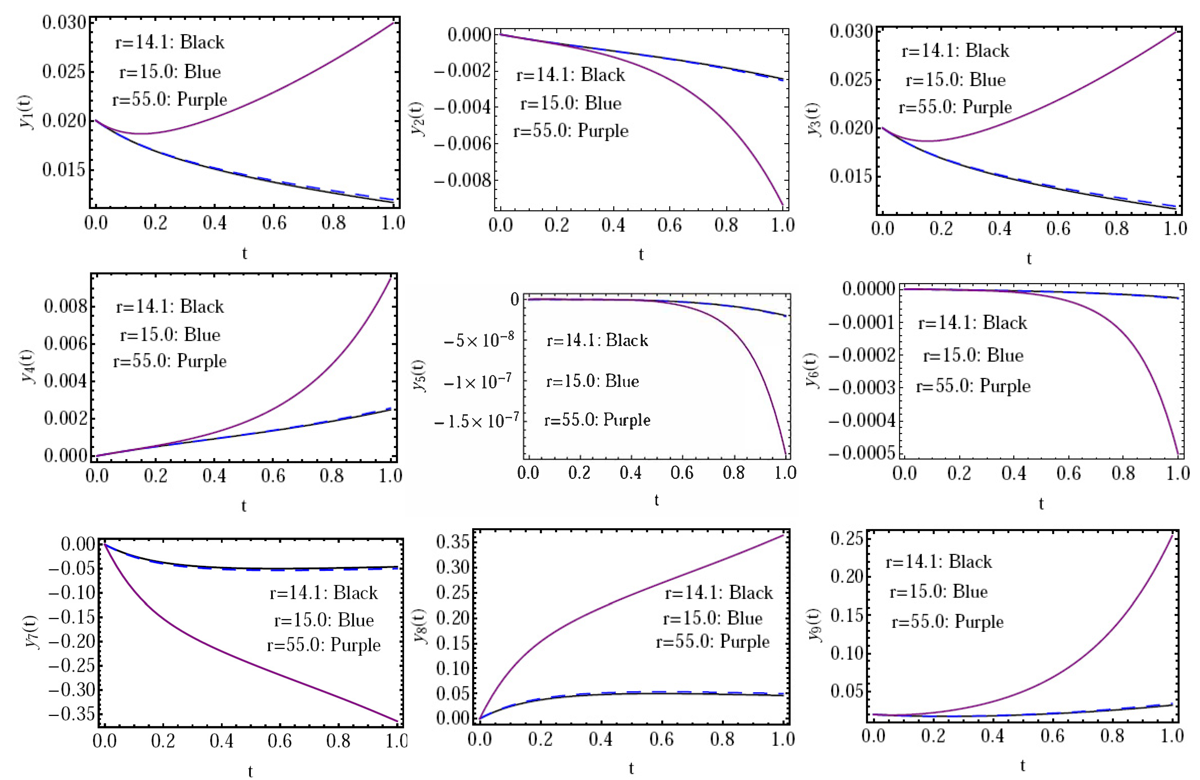
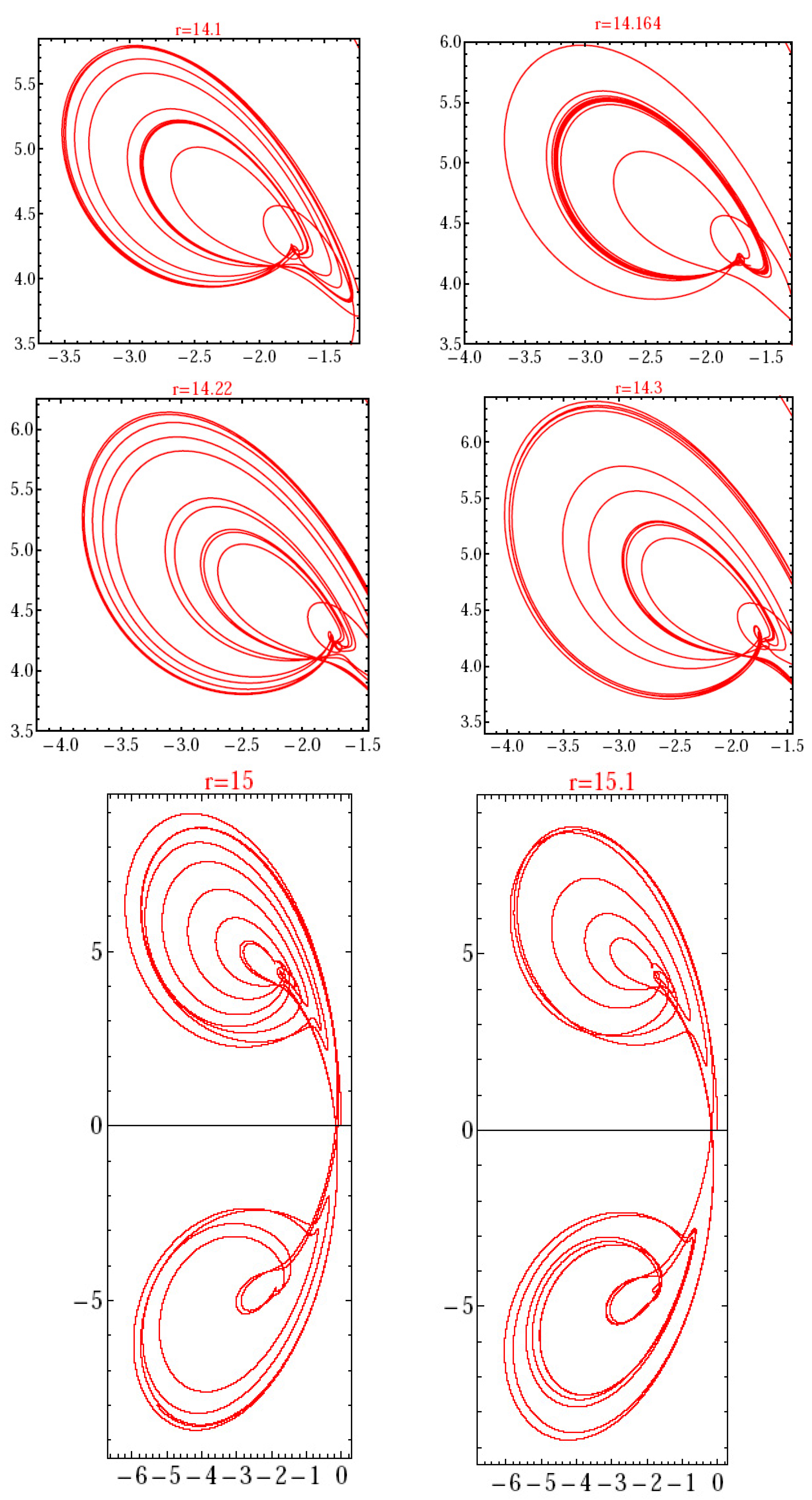
Reiterer et al. [27] noted that, when the value of r is greater than 43.3, the system displays hyper-chaotic behavior, otherwise it is still chaotic. Here, we present both chaotic and hyper-chaotic cases of the solution of the system under study (15)–(24) for values of r between 14.1–15.1 and r = 55, respectively. The numerical results obtained for the studied model by applying the proposed technique are introduced in Figure 1, Figure 2, Figure 3, Figure 4, Figure 5 and Figure 6.

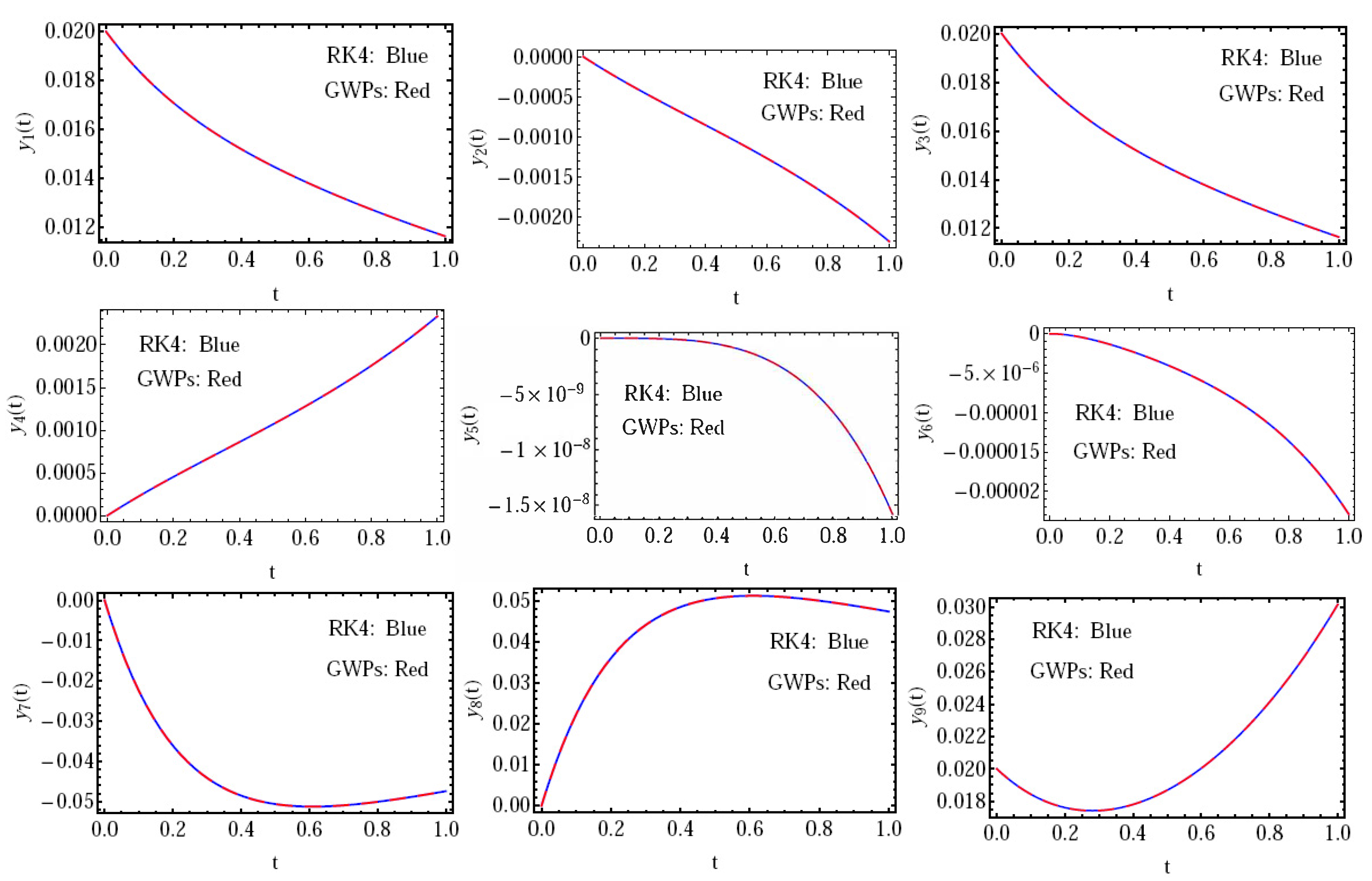
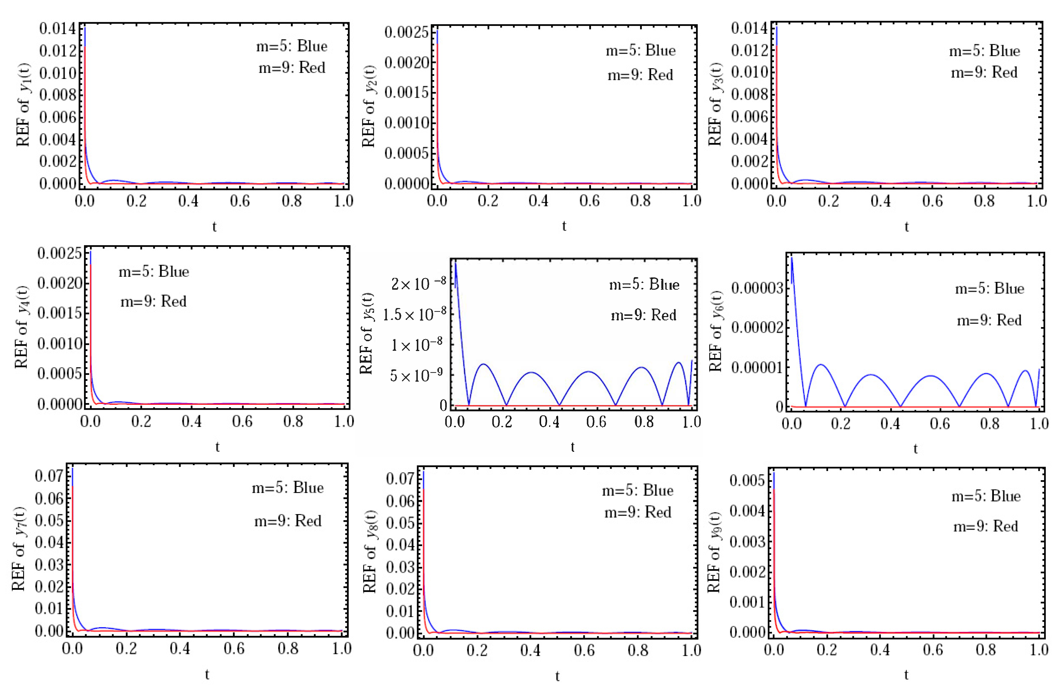
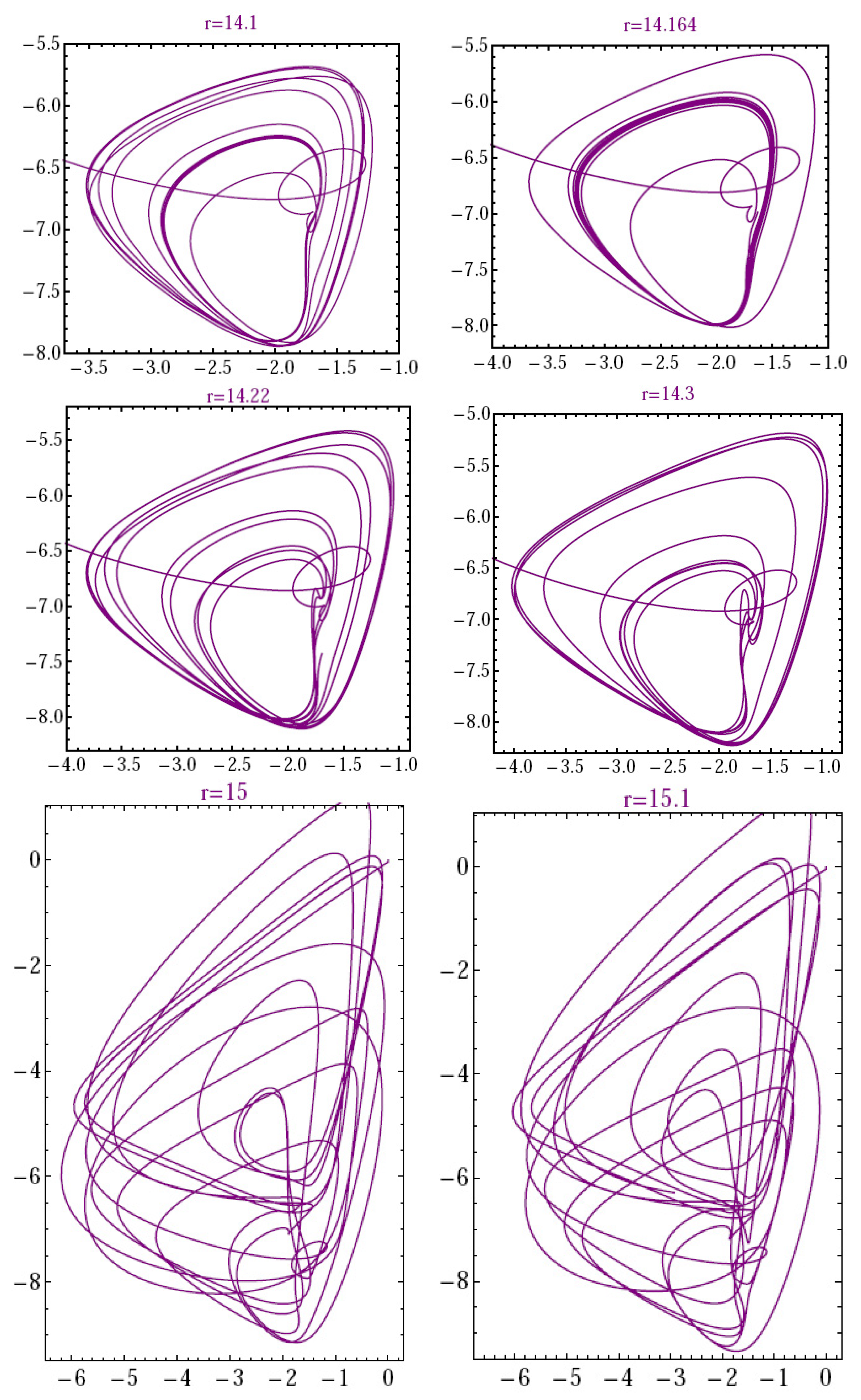
The numerical solution via distinct quantities of $\nu =1.0,0.95,0.85,0.75$, with $m=6,r=14.1$ is given in Figure 1; in Figure 2, we give the numerical solution via different values of $r=14.1,15.0,55.0,$ with $m=7$. Figure 3 presents a comparison between the results obtained by the proposed method with the results that can be obtained by implementing the Runge–Kutta method of order four (RK4) at ($\nu =1$) with $m=6,r=14.1$. Figure 4 represents the residual error function (REF) [28] of the approximate solution at $\nu =0.96,r=14.1$ with different values of $m=5,9$. Finally, in Figure 5 and Figure 6, we present the phase projections on the $y_6-y_7$ and $y_6-y_9$ planes, for different values of r, with $m=8,\nu =0.99$. From these Figure 5 and Figure 6, it can be seen that the obtained phase-portraits are in close agreement with those of Kouagou et al. [29]. This indicates that the technique presented is capable of handling such high-dimensional chaotic systems.

Remark 1.

The chaotic and hyper-chaotic features in these figures depend on the values of the parameter r, which exists in the last three Equations (21)–(23) of the system, so there is a chaotic solution expected in the last four components of the solution. As is known, the Lorenz system has chaotic solutions (but not all the solutions are chaotic).

Through Figure 1, Figure 2, Figure 3 and Figure 4, it can be seen that the behavior of the approximate solution resulting from the application of the proposed method, based on the values of $m,r,$ and $\nu$, confirms that the proposed method is suitable for solving the proposed model in its fractional form with the RFE operator. In addition, the proposed efficient technique improves the accuracy of the results obtained.

5. Conclusions

We investigated the dynamical behavior of the Lorenz mathematical model with the help of the Caputo differential operator and used the utilities of fractional calculus. The numerical solutions of the model under investigation were computed with distinct quantities of the fractional-order, $\nu$, the approximation-order, m, and the REF. In light of these solutions, we can confirm that the proposed procedure is appropriate to effectively simulate the given system. In addition, we can control the accuracy of the error and reduce it by adding additional terms (increasing m) from the approximate solution series. From the numerical solutions that were graphically isolated, we found that they were comparable with those that can be obtained using the RK4 method. The results also showed that the proposed method is computationally accurate and effective and represents a reliable way to solve such complex dynamical models with chaotic and excessive behavior. We can apply the results obtained to investigate various phenomena, including the weather, with many applications in science and engineering. In the future, we will seek to deal with the same model, but using another type of fractional derivative or another type of polynomial as a generalization of this study. We will also investigate the stability and explore the biological applications of the proposed model. The Mathematica software package was used to perform the numerical simulation.

References

- Lorenz, E. Deterministic nonperiodic flow. J. Atmospheric Sci. 1963, 20, 130–141. [Google Scholar] [CrossRef]
- Rossler, O.E. An equation for continuous chaos. Phys. Lett. A 1976, 57, 397–398. [Google Scholar] [CrossRef]
- Ispolatov, I.; Madhok, V.; Allende, S.; Doebeli, M. Chaos in high-dimensional dissipative dynamical systems. Sci. Rep. 2015, 5, 125–135. [Google Scholar] [CrossRef] [PubMed] [Green Version]
- Haken, H. Analogy between higher instabilities in fluids and lasers. Phys. Lett. A 1975, 53, 77–78. [Google Scholar] [CrossRef]
- Edgar, K. Chaos in the segmented disc dynamo. Phys. Lett. A 1981, 82, 439–440. [Google Scholar]
- Gorman, M.; Widmann, P.J.; Robbins, K.A. Nonlinear dynamics of a convection loop: A quantitative comparison of experiment with theory. Physica D 1986, 19, 255–267. [Google Scholar] [CrossRef]
- Kevin, C.M.; Alan, O.V. Circuit implementation of synchronized chaos with applications to communications. Phys. Rev. Lett. 1993, 71, 65–68. [Google Scholar]
- Douglas, P. Cooperative catalysis and chemical chaos: A chemical model for the Lorenz equations. Physica D 1993, 65, 86–99. [Google Scholar]
- Eftekhari, S.A.; Jafari, A.A. Numerical simulation of chaotic dynamical systems by the method of differential quadrature. Sci. Iran. 2012, 19, 1299–1315. [Google Scholar] [CrossRef] [Green Version]
- Odibat, Z.M.; Bertelle, C.; Aziz-Alaoui, M.A.; Duchamp, G.H.E. A multi-step differential transform method and application to non-chaotic or chaotic systems. Comput. Math. Appl. 2010, 59, 1462–1472. [Google Scholar] [CrossRef] [Green Version]
- Zhou, X.; Li, J.; Wang, Y.; Zhang, W. Numerical simulation of a class of hyperchaotic system using Barycentric Lagrange interpolation collocation method. Complexity 2019, 1, 1–13. [Google Scholar] [CrossRef]
- Khader, M.M.; Abualnaja, K.M. Galerkin-FEM for obtaining the numerical solution of the linear fractional Klein-Gordon equation. J. Appl. Anal. Comput. 2019, 9, 261–270. [Google Scholar] [CrossRef]
- Khader, M.M.; Adel, M. Modeling and numerical simulation for covering the fractional COVID-19 model using spectral collocation-optimization algorithms. Fractal Fract. 2022, 6, 363. [Google Scholar] [CrossRef]
- Saad, K.M.; Khader, M.M.; Gomez-Aguilar, J.F.; Baleanu, D. Numerical solutions of the fractional Fisher’s type equations with Atangana-Baleanu fractional derivative by using spectral collocation methods. Chaos 2019, 29, 1–5. [Google Scholar] [CrossRef]
- Adel, M.; Srivastava, H.M.; Khader, M.M. Implementation of an accurate method for the analysis and simulation of electrical R-L circuits. Math. Meth. Appl. Sci. 2022, 12, 1–10. [Google Scholar]
- Liu, Y.; Yin, B.; Li, H.; Zhang, Z. The unified theory of shifted convolution quadrature for fractional calculus. J. Sci. Comput. 2021, 89, 1–24. [Google Scholar] [CrossRef]
- Anjam, Y.N.; Shafqat, R.; Sarris, I.E.; Rahma, M.; Touseef, S.; Arshad, M. A fractional order investigation of smoking model using Caputo-Fabrizio differential operator. Fractal Fract. 2022, 6, 623. [Google Scholar] [CrossRef]
- Iqbal, M.A.; Shakeel, M.; Mohyud-Din, S.T.; Rafiq, M. Modified wavelets-based algorithm for nonlinear delay differential equations of fractional order. Adv. Mech. Eng. 2017, 9, 1–8. [Google Scholar]
- Ozdemir, N.; Secer, A.; Bayram, M. The Gegenbauer wavelets-based computational methods for the coupled system of Burgers’ equations with time-fractional derivative. Mathematics 2019, 7, 486. [Google Scholar] [CrossRef] [Green Version]
- Kilbas, A.A.; Srivastava, H.M.; Trujillo, J.J. Theory and Applications of Fractional Differential Equations; Elsevier: Amsterdam, The Netherlands, 2006; Volume 204. [Google Scholar]
- Saadatmandi, A.; Dehghan, M. A new operational matrix for solving fractional-order differential equations. Comput. Math. Appl. 2010, 59, 1326–1336. [Google Scholar] [CrossRef] [Green Version]
- Celik, I. Generalization of Gegenbauer wavelet collocation method to the generalized Kuramoto-Sivashinsky equation. Int. J. Appl. Comput. Math. 2018, 13, 4–11. [Google Scholar]
- Rehman, M.U.; Saeed, U. Gegenbauer wavelets operational matrix method for fractional differential equations. J. Korean Math. Soc. 2015, 52, 1069–1096. [Google Scholar] [CrossRef] [Green Version]
- Celik, I. Gegenbauer wavelet collocation method for the extended Fisher-Kolmogorov equation in two dimensions. Math. Methods Appl. Sci. 2020, 43, 5615–5628. [Google Scholar] [CrossRef]
- Usman, M.; Hamid, M.; Haq, R.U.; Wang, W. An efficient algorithm based on Gegenbauer wavelets for the solutions of variable-order fractional differential equations. Eur. Phys. J. Plus 2018, 13, 133–150. [Google Scholar] [CrossRef]
- Secer, A.; Ozdemir, N. An effective computational approach based on Gegenbauer wavelets for solving the time-fractional Kdv-Burger’s-Kuramoto equation. Adv. Differ. Equ. 2019, 2019, 389–393. [Google Scholar] [CrossRef]
- Reiterer, P.; Lainscsek, C.; Sch, F.; Maquet, J. A nine-dimensional Lorenz system to study high-dimensional chaos. J. Phys. A Math. Gen. 1998, 31, 7121–7139. [Google Scholar] [CrossRef]
- El-Hawary, H.M.; Salim, M.S.; Hussien, H.S. Ultraspherical integral method for optimal control problems governed by ordinary differential equations. J. Glob. Optim. 2003, 25, 283–303. [Google Scholar] [CrossRef]
- Dlamini, J.N.K.P.G.; Simelane, S.M. On the multi-domain compact finite difference relaxation method for high dimensional chaos: The nine-dimensional Lorenz system. Alex. Eng. J. 2020, 59, 2617–2625. [Google Scholar]
Figure 1.
The approximate solution against distinct values of .
Figure 2.
The approximate solution against distinct values of r.
Figure 3.
The solution by GWPs and RK4 methods .
Figure 4.
The REF of against distinct values of m.
Figure 5.
The hyper-chaotic situation in the case of the plane versus different values of r.
Figure 6.
Disclaimer/Publisher’s Note: The statements, opinions and data contained in all publications are solely those of the individual author(s) and contributor(s) and not of MDPI and/or the editor(s). MDPI and/or the editor(s) disclaim responsibility for any injury to people or property resulting from any ideas, methods, instructions or products referred to in the content. |
© 2023 by the authors. Licensee MDPI, Basel, Switzerland. This article is an open access article distributed under the terms and conditions of the Creative Commons Attribution (CC BY) license (https://creativecommons.org/licenses/by/4.0/).
Share and Cite
MDPI and ACS Style
Alqhtani, M.; Khader, M.M.; Saad, K.M. Numerical Simulation for a High-Dimensional Chaotic Lorenz System Based on Gegenbauer Wavelet Polynomials. Mathematics 2023, 11, 472. https://doi.org/10.3390/math11020472
AMA Style
Alqhtani M, Khader MM, Saad KM. Numerical Simulation for a High-Dimensional Chaotic Lorenz System Based on Gegenbauer Wavelet Polynomials. Mathematics. 2023; 11(2):472. https://doi.org/10.3390/math11020472
Chicago/Turabian StyleAlqhtani, Manal, Mohamed M. Khader, and Khaled Mohammed Saad. 2023. "Numerical Simulation for a High-Dimensional Chaotic Lorenz System Based on Gegenbauer Wavelet Polynomials" Mathematics 11, no. 2: 472. https://doi.org/10.3390/math11020472
Note that from the first issue of 2016, this journal uses article numbers instead of page numbers. See further details here.