Modeling and Stability Analysis of Within-Host IAV/SARS-CoV-2 Coinfection with Antibody Immunity

Abstract

Studies have reported several cases with respiratory viruses coinfection in hospitalized patients. Influenza A virus (IAV) mimics the Severe Acute Respiratory Syndrome Coronavirus 2 (SARS-CoV-2) with respect to seasonal occurrence, transmission routes, clinical manifestations and related immune responses. The present paper aimed to develop and investigate a mathematical model to study the dynamics of IAV/SARS-CoV-2 coinfection within the host. The influence of SARS-CoV-2-specific and IAV-specific antibody immunities is incorporated. The model simulates the interaction between seven compartments, uninfected epithelial cells, SARS-CoV-2-infected cells, IAV-infected cells, free SARS-CoV-2 particles, free IAV particles, SARS-CoV-2-specific antibodies and IAV-specific antibodies. The regrowth and death of the uninfected epithelial cells are considered. We study the basic qualitative properties of the model, calculate all equilibria and investigate the global stability of all equilibria. The global stability of equilibria is established using the Lyapunov method. We perform numerical simulations and demonstrate that they are in good agreement with the theoretical results. The importance of including the antibody immunity into the coinfection dynamics model is discussed. We have found that without modeling the antibody immunity, the case of IAV and SARS-CoV-2 coexistence is not observed. Finally, we discuss the influence of IAV infection on the dynamics of SARS-CoV-2 single-infection and vice versa.

1. Introduction

Coronavirus disease 2019 (COVID-19) was detected in December 2019, in Wuhan, China during the season when influenza was still circulating [1]. COVID-19 is caused by a dangerous type of virus called severe acute respiratory syndrome coronavirus 2 (SARS-CoV-2). According to the update provided by the World Health Organization (WHO) on 21 August 2022 [2], over 593 million confirmed cases and over 6.4 million deaths have been reported globally. SARS-CoV-2 is transmitted to people when they are exposed to respiratory fluids carrying infectious viral particles. The implementation of preventive measures such as physical and social distancing, using face masks, hand washing, disinfection of surfaces and getting vaccinated can reduce SARS-CoV-2 transmission. Eleven vaccines for COVID-19 have been approved by WHO for emergency use. These include Novavax, CanSino, Bharat Biotech, Pfizer/BioNTech, Moderna, Serum Institute of India (Novavax formulation), Janssen (Johnson & Johnson), Oxford/AstraZeneca, Serum Institute of India (Oxford/AstraZeneca formulation), Sinopharm and Sinovac [3]. SARS-CoV-2 is a single-stranded positive-sense RNA virus that infects the epithelial cells. SARS-CoV-2 can cause an acute respiratory distress syndrome (ARDS), which has high mortality rates, particularly in patients with immunosenescence [4]. Immunosenescence renders vaccination less effective and increases the susceptibility to viral infections [5].

Influenza viruses are members of the family of Orthomyxoviridae, which are negativesense RNA viruses. There are four distinct influenza viruses, A, B, C and D. Influenza A virus (IAV) can infect a wide range of species. IAV is a significant public health threat, resulting in 15-65 million infections and over 200,000 hospitalizations every year during seasonal epidemics in the United States [6]. IAV infects the uninfected epithelial cells of the host respiratory tract [7]. Both SARS-CoV-2 and IAV have analogous transmission ways, moreover, they have common clinical manifestations including dyspnea, cough, fever, headache, rhinitis, myalgia and sore throat [1]. Viral shedding usually takes place 5 to 10 days in influenza, whereas it does 2 to 5 weeks in COVID-19 [1]. Acute respiratory distress is less common in influenza than COVID-19 [1]. Deaths in influenza cases are less than 1%, while in cases of COVID-19 it ranges from 3% to 4% [1].

It was reported in [8] that 94.2% of individuals with COVID-19 were also coinfected with several other microorganisms, such as fungi, bacteria and viruses. Important viral copathogens include the respiratory syncytial virus (RSV), human enterovirus (HEV), human rhinovirus (HRV), influenza A virus (IAV), influenza B virus (IBV), human metapneumovirus (HMPV), parainfluenza virus (PIV), human immunodeficiency virus (HIV), cytomegalovirus (CMV), dengue virus (DENV), Epstein Barr virus (EBV), hepatitis B virus (HBV) and other coronaviruses (COVs), among which the HRV, HEV and IAV are the most common copathogens [9]. Several coinfection cases of COVID-19 and influenza have been reported in [1,8,10,11,12] (see also the review papers [13,14,15,16]). Based on two separate studies presented in [10,11], COVID-19-influenza coinfection did not result in worse clinical outcomes [10]. In addition, this condition reduced the mortality rate among COVID-19-influenza coinfected patients. Coinfection with influenza virus in COVID-19 patients might render them less vulnerable to morbidities associated with COVID-19, and therefore, a better prognosis overall [11]. In [16], it was found that, although patients with IAV and SARS-CoV-2 coinfection did not experience longer hospital stays compared with those with a SARS COV-2 single-infection, they usually presented with more severe clinical conditions.

Viral interference phenomenon can appear in case of infections with multiple competitive respiratory viruses. One virus may be able to suppress the growth of another virus [17,18,19]. Disease progression and outcome in SARS-CoV-2 infection are highly dependent on the host immune response, particularly in the elderly in whom immunosenescence may predispose to increased risk of coinfection [17].

Over the years, mathematical models have demonstrated their ability to provide useful insight to gain a further understanding of the dynamics and mechanisms of the viruses within a host level. These models may assist in the development of viral therapies and vaccines as well as the selection of appropriate therapeutic and vaccine strategies. Moreover, these models are helpful in determining the sufficient number of factors to analyze the experimental results and explain the biological phenomena [7]. Stability analysis of the model’s equilibria can help researchers (i) to expect the qualitative features of the model for a given set of values of the model’s parameters, (ii) to establish the conditions that ensure the persistence or deletion of this infection, and (iii) to determine under what conditions the immune system is stimulated against the infection. Mathematical models of within-host IAV single-infection have been developed in several works. Baccam et al. [20] presented the following IAV-single-infection with limited target cells:

$$\left\{\begin{array}{c}\dot{X}=-\stackrel{\mathrm{IAV}\mathrm{infectious}\mathrm{transmission}}{\overbrace{\beta XP}},\hfill \\ \dot{I}=\stackrel{\mathrm{IAV}\mathrm{infectious}\mathrm{transmission}}{\overbrace{\beta XP}}-\stackrel{\mathrm{natural}\mathrm{death}}{\overbrace{\gamma I}},\hfill \\ \dot{P}=\stackrel{\mathrm{IAV}\mathrm{production}}{\overbrace{\kappa I}}-\stackrel{\mathrm{natural}\mathrm{death}}{\overbrace{\pi P}},\hfill \end{array}\right.$$

(1)

where $X=X\left(t\right)$, $I=I\left(t\right)$ and $P=P\left(t\right)$ are the concentrations of uninfected epithelial cells, IAV-infected epithelial cells and free IAV particles, at time t, respectively. The model was fitted using real data from six patients infected with influenza [20].

Several works have been devoted to study IAV single-infection dynamics models (see the review papers [21,22,23,24]) by including the effect of innate immune response [20,25], adaptive immune response [26,27] and both innate and adaptive immune responses [5,7,28,29,30]. Handel et al. [31] presented a mathematical model for within-host influenza infection under the effect of neuraminidase inhibitors drugs. The effect of a combination of neuraminidase inhibitors and anti-IAV therapies was addressed in [26]. In [26], the first equation of model (1) was modified by considering the target cell production and death as:

$$\dot{X}=\stackrel{\mathrm{epithelial}\mathrm{cells}\mathrm{production}}{\overbrace{\alpha X\left(0\right)}}-\stackrel{\mathrm{natural}\mathrm{death}}{\overbrace{\alpha X}}-\stackrel{\mathrm{IAV}\mathrm{infectious}\mathrm{transmission}}{\overbrace{\beta XP}},$$

(2)

where $X\left(0\right)$ is the initial concentration of the uninfected epithelial cells.

Model (1) was utilized to characterize the dynamics of SARS-CoV-2 within a host in [32]. Li et al. [33] used Equation (2) for the SARS-CoV-2 infection dynamics. A model with target-cell limited and a model with regrowth and death of the uninfected epithelial cells presented, respectively, in [32,33] were extended and modified by including (i) latently infected epithelial cells [32,34,35,36], (ii) effect of immune response [37,38,39,40,41,42], (iii) effect of different drug therapies [35,43,44], and (iv) effect of time delay [45].

Recently, several mathematical models have been developed to characterize the coinfection of COVID-19 with other diseases in epidemiology (between-host), such as COVID-19/HIV [46], COVID-19/Dengue [47], COVID-19/Dengue/HIV [48], COVID-19/ZIKV [49], COVID-19/Bacterial [50], COVID-19/Influenza [51] and COVID-19/Tuberculosis [52]. However, modeling of within-host dynamics of COVID-19 with other pathogen coinfection has been investigated in few papers: SARS-CoV-2/HIV [53], SARS-CoV-2/malaria [54] and SARS-CoV-2/Bacteria [55]. Based on the target cell-limited model (1), Pinky and Dobrovolny [18,19] developed a model for the within-host dynamics of two respiratory viruses coinfection. They suggested that several types of respiratory viruses can suppress the SARS-CoV-2 infection.

The model presented in [18,19] describes the competition between two respiratory viruses. However, the impact of the immune response against the two viruses was not modeled. Further, the regeneration and death of the uninfected epithelial cells were neglected. Furthermore, mathematical analysis of the model was not studied. Therefore, the aim of the present paper is to develop a within-host IAV/SARS-CoV-2 coinfection model with immune response. The model is a generalization of the model presented in [18,19] by incorporating (i) the regrowth and death of the uninfected epithelial cells, and (ii) the impact of SARS-CoV-2-specific antibody and IAV-specific antibody. We study the basic qualitative properties of the proposed model, calculate all equilibria and investigate the global stability of the equilibria. We support our theoretical results via numerical simulations. Finally, we discuss the obtained results.

Our proposed model can be useful to describe the within-host dynamics of coinfection with two or more viral strains, or coinfection of SARS-CoV-2 (or IAV) and other respiratory viruses. Moreover, the model may help to predict new treatment regimens for viral coinfections.

2. Model Formulation

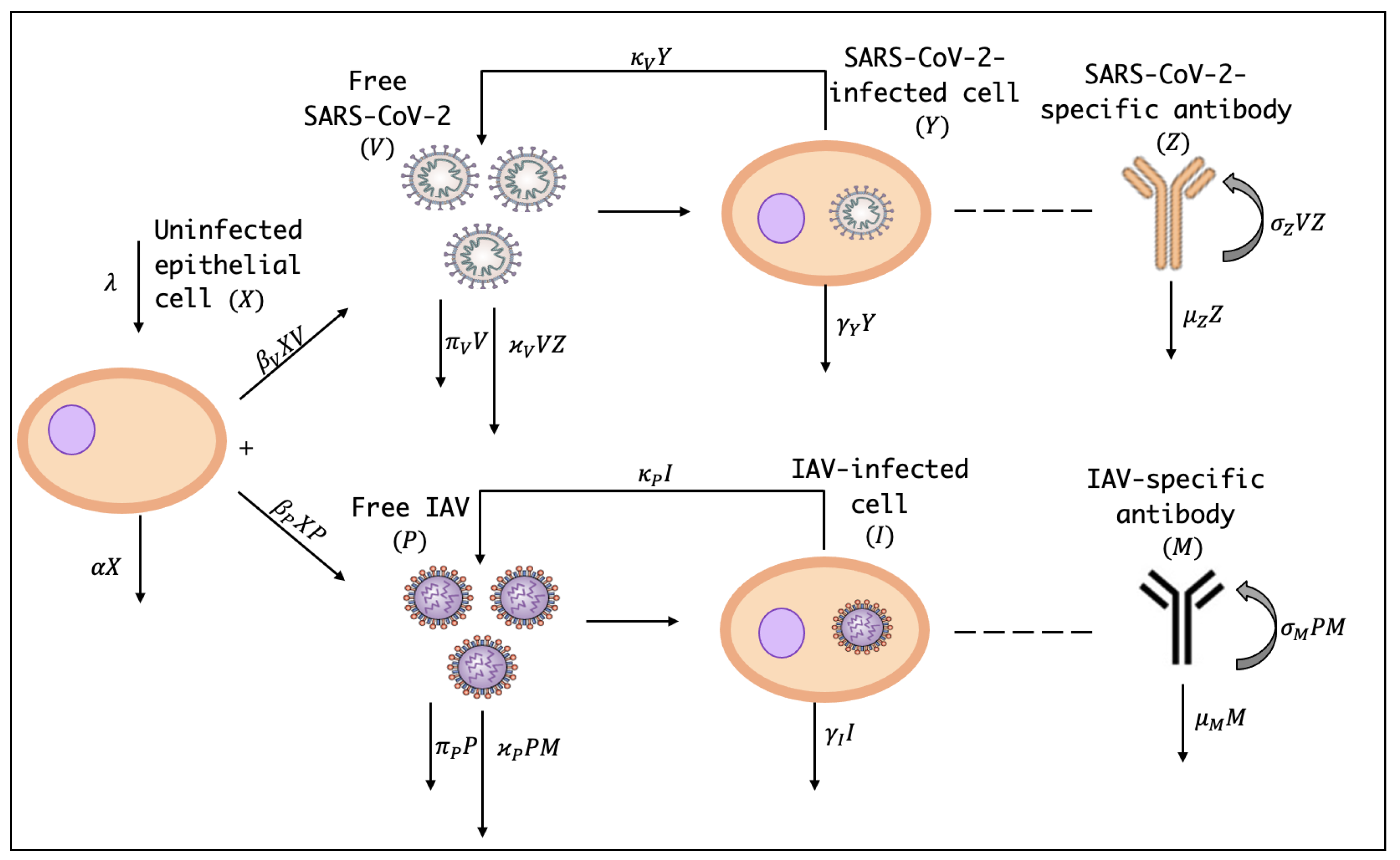
In this section, we present an IAV/SARS-CoV-2 coinfection dynamics model. The dynamics of IAV/SARS-CoV-2 coinfection is presented in the diagram Figure 1. Let us consider following assumptions:

A1

The model considers the interactions between seven compartments: uninfected epithelial cells (X), SARS-CoV-2-infected cells (Y), IAV-infected cells (I), free SARS-CoV-2 particles (V), free IAV particles (P), SARS-CoV-2-specific antibodies (Z) and IAV-specific antibodies (M). Here, X, Y, I, V, P, Z and M represent the concentrations of the seven compartments.

A2

The uninfected epithelial cells are the target for both SARS-CoV-2 and IAV [18,20,32].

A3

The uninfected epithelial cells are regenerated and die at rates $\lambda$ and $\alpha X$, respectively [33,40,42,56].

A4

The SARS-CoV-2-specific antibodies proliferate at rate ${\sigma }_{Z}VZ$, decay at rate ${\mu }_{Z}Z$ and neutralize the SARS-CoV-2 particles at rate ${\varkappa }_{V}VZ$ [45,57].

A5

The IAV-specific antibodies proliferate at rate ${\sigma }_{M}PM$, decay at rate ${\mu }_{M}M$ and neutralize the IAV particles at rate ${\varkappa }_{P}PM$ [56].

Based on Assumptions A1–A5, we formulate the IAV/SARS-CoV-2 coinfection dynamics model as:

$$\left\{\begin{array}{c}\dot{X}=\stackrel{\mathrm{epithelial}\mathrm{cells}\mathrm{production}}{\overbrace{\lambda }}-\stackrel{\mathrm{natural}\mathrm{death}}{\overbrace{\alpha X}}-\stackrel{\mathrm{SARS}-\mathrm{CoV}-2\mathrm{infectious}\mathrm{transmission}}{\overbrace{{\beta }_{V}XV}}-\stackrel{\mathrm{IAV}\mathrm{infectious}\mathrm{transmission}}{\overbrace{{\beta }_{P}XP}},\hfill \\ \dot{Y}=\stackrel{\mathrm{SARS}-\mathrm{CoV}-2\mathrm{infectious}\mathrm{transmission}}{\overbrace{{\beta }_{V}XV}}-\stackrel{\mathrm{natural}\mathrm{death}}{\overbrace{{\gamma }_{Y}Y}},\hfill \\ \dot{I}=\stackrel{\mathrm{IAV}\mathrm{infectious}\mathrm{transmission}}{\overbrace{{\beta }_{P}XP}}-\stackrel{\mathrm{natural}\mathrm{death}}{\overbrace{{\gamma }_{I}I}},\hfill \\ \dot{V}=\stackrel{\mathrm{SARS}-\mathrm{CoV}-2\mathrm{production}}{\overbrace{{\kappa }_{V}Y}}-\stackrel{\mathrm{natural}\mathrm{death}}{\overbrace{{\pi }_{V}V}}-\stackrel{\mathrm{SARS}-\mathrm{CoV}-2\mathrm{neutralization}}{\overbrace{{\varkappa }_{V}VZ}},\hfill \\ \dot{P}=\stackrel{\mathrm{IAV}\mathrm{production}}{\overbrace{{\kappa }_{P}I}}-\stackrel{\mathrm{natural}\mathrm{death}}{\overbrace{{\pi }_{P}P}}-\stackrel{\mathrm{IAV}\mathrm{neutralization}}{\overbrace{{\varkappa }_{P}PM}},\hfill \\ \dot{Z}=\stackrel{\mathrm{SARS}-\mathrm{CoV}-2-\mathrm{specific}\mathrm{antibody}\mathrm{proliferation}}{\overbrace{{\sigma }_{Z}VZ}}-\stackrel{\mathrm{natural}\mathrm{death}}{\overbrace{{\mu }_{Z}Z}},\hfill \\ \dot{M}=\stackrel{\mathrm{IAV}-\mathrm{specific}\mathrm{antibody}\mathrm{proliferation}}{\overbrace{{\sigma }_{M}PM}}-\stackrel{\mathrm{natural}\mathrm{death}}{\overbrace{{\mu }_{M}M}}.\hfill \end{array}\right.$$

(3)

3. Basic Qualitative Properties

In this section, we study the basic qualitative properties of system (3). We establish the nonnegativity and boundedness of the system’s solutions to ensure that our model is biologically acceptable. Particularly, the concentrations of the model’s compartments should not become negative or unbounded.

Lemma 1.

The solutions of system (3) are nonnegative and bounded.

Proof. 

We have that

$$\begin{array}{cc}\hfill \dot{X}& {\mid }_{X=0}=\lambda >0,\dot{Y}{\mid }_{Y=0}={\beta }_{V}XV\ge 0\mathrm{for}\mathrm{all}X,V\ge 0,\hfill \\ \hfill \dot{I}& {\mid }_{I=0}={\beta }_{P}XP\ge 0\mathrm{for}\mathrm{all}X,P\ge 0,\dot{V}{\mid }_{V=0}={\kappa }_{V}Y\ge 0\mathrm{for}\mathrm{all}Y\ge 0,\hfill \\ \hfill \dot{P}& {\mid }_{P=0}={\kappa }_{P}I\ge 0\mathrm{for}\mathrm{all}I\ge 0,\hfill \\ \hfill \dot{Z}& {\mid }_{Z=0}=0,\dot{M}{\mid }_{M=0}=0.\hfill \end{array}$$

This guarantees that $(X\left(t\right),Y\left(t\right),I\left(t\right),V\left(t\right),P\left(t\right),Z\left(t\right),M\left(t\right))\in {\mathbb{R}}_{\ge 0}^7$ for all $t\ge 0$ when $(X\left(0\right),Y\left(0\right),I\left(0\right),V\left(0\right),P\left(0\right),Z\left(0\right),M\left(0\right))\in {\mathbb{R}}_{\ge 0}^7$. Let us define

$$\Psi =X+Y+I+\frac{{\gamma }_Y}{2{\kappa }_V}V+\frac{{\gamma }_I}{2{\kappa }_P}P+\frac{{\gamma }_Y{\varkappa }_V}{2{\kappa }_V{\sigma }_Z}Z+\frac{{\gamma }_I{\varkappa }_P}{2{\kappa }_P{\sigma }_M}M.$$

Then,

$$\begin{array}{cc}\hfill \dot{\Psi }& =\lambda -\alpha X-\frac{{\gamma }_Y}{2}Y-\frac{{\gamma }_I}{2}I-\frac{{\gamma }_Y{\pi }_V}{2{\kappa }_V}V-\frac{{\gamma }_I{\pi }_P}{2{\kappa }_P}P-\frac{{\gamma }_Y{\varkappa }_V{\mu }_Z}{2{\kappa }_V{\sigma }_Z}Z-\frac{{\gamma }_I{\varkappa }_P{\mu }_M}{2{\kappa }_P{\sigma }_M}M\hfill \\ \hfill & \le \lambda -\varphi \left[X+Y+I+\frac{{\gamma }_Y}{2{\kappa }_V}V+\frac{{\gamma }_I}{2{\kappa }_P}P+\frac{{\gamma }_Y{\varkappa }_V}{2{\kappa }_V{\sigma }_Z}Z+\frac{{\gamma }_I{\varkappa }_P}{2{\kappa }_P{\sigma }_M}M\right]=\lambda -\varphi \Psi ,\hfill \end{array}$$

where $\varphi =min\{\alpha ,\frac{{\gamma }_Y}{2},\frac{{\gamma }_I}{2},{\pi }_V,{\pi }_P,{\mu }_Z,{\mu }_M\}$. Thus, $0\le \Psi \left(t\right)\le {\Delta }_1$ if $\Psi \left(0\right)\le {\Delta }_1$ for $t\ge 0,$ where ${\Delta }_1=\frac{\lambda }{\varphi }.$ Since $X,Y,I,V,P,Z$ and M are all nonnegative, then $0\le X\left(t\right),Y\left(t\right),I\left(t\right)\le {\Delta }_1$, $0\le V\left(t\right)\le {\Delta }_2$, $0\le P\left(t\right)\le {\Delta }_3$, $0\le Z\left(t\right)\le {\Delta }_4$, $0\le M\left(t\right)\le {\Delta }_5$ if $X\left(0\right)+Y\left(0\right)+I\left(0\right)+\frac{{\gamma }_Y}{2{\kappa }_V}V\left(0\right)+\frac{{\gamma }_I}{2{\kappa }_P}P\left(0\right)+\frac{{\gamma }_Y{\varkappa }_V}{2{\kappa }_V{\sigma }_Z}Z\left(0\right)+\frac{{\gamma }_I{\varkappa }_P}{2{\kappa }_P{\sigma }_M}M\left(0\right)\le {\Delta }_1$, where ${\Delta }_2=\frac{2{\kappa }_V}{{\gamma }_Y}{\Delta }_1$, ${\Delta }_3=\frac{2{\kappa }_P}{{\gamma }_I}{\Delta }_1$, ${\Delta }_4=\frac{2{\kappa }_V{\sigma }_Z}{{\gamma }_Y{\varkappa }_V}{\Delta }_1$ and ${\Delta }_5=\frac{2{\kappa }_P{\sigma }_M}{{\gamma }_I{\varkappa }_P}{\Delta }_1$. This proves the boundedness of the solutions. □

4. Equilibria

In this section, we are interested in the conditions of existence of the system’s equilibria. Moreover, we derive a set of threshold parameters which govern the existence of equilibria. At any equilibrium $\Xi =(X,Y,I,V,P,Z,M)$, the following equations hold:

$$\begin{array}{cc}\hfill 0& =\lambda -\alpha X-{\beta }_{V}XV-{\beta }_{P}XP,\hfill \end{array}$$

(4)

$$\begin{array}{cc}\hfill 0& ={\beta }_{V}XV-{\gamma }_{Y}Y,\hfill \end{array}$$

(5)

$$\begin{array}{cc}\hfill 0& ={\beta }_{P}XP-{\gamma }_{I}I,\hfill \end{array}$$

(6)

$$\begin{array}{cc}\hfill 0& ={\kappa }_{V}Y-{\pi }_{V}V-{\varkappa }_{V}VZ,\hfill \end{array}$$

(7)

$$\begin{array}{cc}\hfill 0& ={\kappa }_{P}I-{\pi }_{P}P-{\varkappa }_{P}PM,\hfill \end{array}$$

(8)

$$\begin{array}{cc}\hfill 0& ={\sigma }_{Z}VZ-{\mu }_{Z}Z,\hfill \end{array}$$

(9)

$$\begin{array}{cc}\hfill 0& ={\sigma }_{M}PM-{\mu }_{M}M.\hfill \end{array}$$

(10)

Solving Equations (4)–(10), we obtain eight equilibria.

(i) Infection-free equilibrium, ${\Xi }_0=(X_0,0,0,0,0,0,0)$, where $X_0=\lambda /\alpha$.

(ii) SARS-CoV-2 single-infection equilibrium without antibody immunity ${\Xi }_1=(X_1,Y_1,$$0,V_1,0,0,0),$ where

$$X_1=\frac{{\gamma }_Y{\pi }_V}{{\kappa }_V{\beta }_V},Y_1=\frac{\alpha {\pi }_V}{{\kappa }_V{\beta }_V}\left[\frac{X_0{\kappa }_V{\beta }_V}{{\pi }_V{\gamma }_Y}-1\right],V_1=\frac{\alpha }{{\beta }_V}\left[\frac{X_0{\kappa }_V{\beta }_V}{{\pi }_V{\gamma }_Y}-1\right]$$

Therefore, $Y_1>0$ and $V_1>0$ when

$$\frac{X_0{\kappa }_V{\beta }_V}{{\pi }_V{\gamma }_Y}>1.$$

We define the basic SARS-CoV-2 single-infection reproductive ratio as:

$${\Re }_1=\frac{X_0{\kappa }_V{\beta }_V}{{\pi }_V{\gamma }_Y}.$$

The parameter ${\Re }_1$ determines whether or not a SARS-CoV-2 single-infection can be established. Thus, we can write

$$X_1=\frac{X_0}{{\Re }_1},Y_1=\frac{\alpha {\pi }_V}{{\kappa }_V{\beta }_V}\left({\Re }_1-1\right),V_1=\frac{\alpha }{{\beta }_V}\left({\Re }_1-1\right).$$

It follows that, ${\Xi }_1$ exists if ${\Re }_1>1.$

(iii) IAV single-infection equilibrium without antibody immunity, ${\Xi }_2=(X_2,0,I_2,0,P_2,$$0,0)$, where

$$X_2=\frac{{\gamma }_I{\pi }_P}{{\kappa }_P{\beta }_P},I_2=\frac{\alpha {\pi }_P}{{\kappa }_P{\beta }_P}\left[\frac{X_0{\kappa }_P{\beta }_P}{{\pi }_P{\gamma }_I}-1\right],P_2=\frac{\alpha }{{\beta }_P}\left[\frac{X_0{\kappa }_P{\beta }_P}{{\pi }_P{\gamma }_I}-1\right].$$

Therefore, $I_2>0$ and $P_2>0$ when

$$\frac{X_0{\kappa }_P{\beta }_P}{{\pi }_P{\gamma }_I}>1.$$

We define the basic IAV-infection reproductive ratio as:

$${\Re }_2=\frac{X_0{\kappa }_P{\beta }_P}{{\pi }_P{\gamma }_I}.$$

The parameter ${\Re }_2$ determines whether or not the IAV single-infection can be established. In terms of ${\Re }_2$, we can write

$$X_2=\frac{X_0}{{\Re }_2},I_2=\frac{\alpha {\pi }_P}{{\kappa }_P{\beta }_P}\left({\Re }_2-1\right),P_2=\frac{\alpha }{{\beta }_P}\left({\Re }_2-1\right).$$

Therefore, ${\Xi }_2$ exists if ${\Re }_2>1$.

(iv) SARS-CoV-2 single-infection equilibrium with stimulated SARS-CoV-2-specific antibody immunity, ${\Xi }_3=(X_3,Y_3,0,V_3,0,Z_3,0)$, where

$$\begin{array}{cc}\hfill X_3& =\frac{\lambda {\sigma }_Z}{{\beta }_V{\mu }_Z+\alpha {\sigma }_Z},Y_3=\frac{\lambda {\beta }_V{\mu }_Z}{{\gamma }_Y\left({\beta }_V{\mu }_Z+\alpha {\sigma }_Z\right)},\hfill \\ \hfill V_3& =\frac{{\mu }_Z}{{\sigma }_Z},Z_3=\frac{{\pi }_V}{{\varkappa }_V}\left[\frac{\lambda {\beta }_V{\sigma }_Z{\kappa }_V}{{\gamma }_Y{\pi }_V({\beta }_V{\mu }_Z+\alpha {\sigma }_Z)}-1\right].\hfill \end{array}$$

We note that ${\Xi }_3$ exists when

$$\frac{\lambda {\beta }_V{\sigma }_Z{\kappa }_V}{{\gamma }_Y{\pi }_V({\beta }_V{\mu }_Z+\alpha {\sigma }_Z)}>1.$$

The SARS-CoV-2-specific antibody activation ratio in case of SARS-CoV-2 single-infection is stated as:

$${\Re }_3=\frac{\lambda {\beta }_V{\sigma }_Z{\kappa }_V}{{\gamma }_Y{\pi }_V({\beta }_V{\mu }_Z+\alpha {\sigma }_Z)}.$$

Thus, $Z_3=\frac{{\pi }_V}{{\varkappa }_V}\left({\Re }_3-1\right)$. The parameter ${\Re }_3$ determines whether or not the SARS-CoV-2-specific antibody immunity is activated in the absence of IAV infection.

(v) IAV single-infection equilibrium with stimulated IAV-specific antibody immunity, ${\Xi }_4=(X_4,0,I_4,0,P_4,0,M_4)$, where

$$\begin{array}{cc}\hfill X_4& =\frac{\lambda {\sigma }_M}{{\beta }_P{\mu }_M+\alpha {\sigma }_M},I_4=\frac{\lambda {\beta }_P{\mu }_M}{{\gamma }_I({\beta }_P{\mu }_M+\alpha {\sigma }_M)},\hfill \\ \hfill P_4& =\frac{{\mu }_M}{{\sigma }_M},M_4=\frac{{\pi }_P}{{\varkappa }_P}\left[\frac{\lambda {\beta }_P{\sigma }_M{\kappa }_P}{{\gamma }_I{\pi }_P({\beta }_P{\mu }_M+\alpha {\sigma }_M)}-1\right].\hfill \end{array}$$

We note that ${\Xi }_4$ exists when

$$\frac{\lambda {\beta }_P{\sigma }_M{\kappa }_P}{{\gamma }_I{\pi }_P({\beta }_P{\mu }_M+\alpha {\sigma }_M)}>1.$$

The IAV-specific antibody immunity activation ratio for IAV single-infection is stated as:

$${\Re }_4=\frac{\lambda {\beta }_P{\sigma }_M{\kappa }_P}{{\gamma }_I{\pi }_P({\beta }_P{\mu }_M+\alpha {\sigma }_M)}.$$

Thus, $M_4=\frac{{\pi }_P}{{\varkappa }_P}\left({\Re }_4-1\right)$. The parameter ${\Re }_4$ determines whether or not the IAV-specific antibody immunity is activated in the absence of SARS-CoV-2 infection.

(vi) IAV/SARS-CoV-2 coinfection equilibrium with only stimulated SARS-CoV-2-specific antibody immunity, ${\Xi }_5=(X_5,Y_5,I_5,V_5,P_5,Z_5,0)$, where

$$\begin{array}{cc}\hfill X_5& =\frac{{\gamma }_I{\pi }_P}{{\kappa }_P{\beta }_P}=X_2,Y_5=\frac{{\beta }_V{\mu }_Z}{{\gamma }_Y{\sigma }_Z}{X}_5,\hfill \\ \hfill I_5& =\frac{{\pi }_P({\beta }_V{\mu }_Z+\alpha {\sigma }_Z)}{{\beta }_P{\sigma }_Z{\kappa }_P}\left[\frac{\lambda {\beta }_P{\kappa }_P{\sigma }_Z}{{\gamma }_I{\pi }_P({\beta }_V{\mu }_Z+\alpha {\sigma }_Z)}-1\right],V_5=\frac{{\mu }_Z}{{\sigma }_Z}=V_3,\hfill \\ \hfill P_5& =\frac{{\beta }_V{\mu }_Z+\alpha {\sigma }_Z}{{\beta }_P{\sigma }_Z}\left[\frac{\lambda {\beta }_P{\kappa }_P{\sigma }_Z}{{\gamma }_I{\pi }_P({\beta }_V{\mu }_Z+\alpha {\sigma }_Z)}-1\right],\hfill \\ \hfill Z_5& =\frac{{\pi }_V}{{\varkappa }_V}\left[\frac{{\pi }_P{\beta }_V{\kappa }_V{\gamma }_I}{{\pi }_V{\beta }_P{\kappa }_P{\gamma }_Y}-1\right]=\frac{{\pi }_V}{{\varkappa }_V}\left({\Re }_1/{\Re }_2-1\right).\hfill \end{array}$$

We note that ${\Xi }_5$ exists when,

$$\frac{{\Re }_1}{{\Re }_2}>1\mathrm{and}\frac{\lambda {\beta }_P{\kappa }_P{\sigma }_Z}{{\gamma }_I{\pi }_P({\beta }_V{\mu }_Z+\alpha {\sigma }_Z)}>1.$$

The SARS-CoV-2 infection reproductive ratio in the presence of IAV infection is stated as:

$${\Re }_5=\frac{\lambda {\beta }_P{\kappa }_P{\sigma }_Z}{{\gamma }_I{\pi }_P({\beta }_V{\mu }_Z+\alpha {\sigma }_Z)}.$$

The parameter ${\Re }_5$ determines whether or not SARS-CoV-2 infected patients could be coinfected with IAV. Hence,

$$I_5=\frac{{\pi }_P({\beta }_V{\mu }_Z+\alpha {\sigma }_Z)}{{\beta }_P{\sigma }_Z{\kappa }_P}\left({\Re }_5-1\right),P_5=\frac{{\beta }_V{\mu }_Z+\alpha {\sigma }_Z}{{\beta }_P{\sigma }_Z}\left({\Re }_5-1\right).$$

and then ${\Xi }_5$ exists if $\frac{{\Re }_1}{{\Re }_2}>1$ and ${\Re }_5>1.$

(vii) IAV/SARS-CoV-2 coinfection equilibrium with only stimulated IAV-specific antibody immunity, ${\Xi }_6=(X_6,Y_6,I_6,V_6,P_6,0,M_6)$, where

$$\begin{array}{cc}\hfill X_6& =\frac{{\gamma }_Y{\pi }_V}{{\kappa }_V{\beta }_V},Y_6=\frac{{\pi }_V({\beta }_P{\mu }_M+\alpha {\sigma }_M)}{{\beta }_V{\sigma }_M{\kappa }_V}\left[\frac{\lambda {\beta }_V{\kappa }_V{\sigma }_M}{{\gamma }_Y{\pi }_V({\beta }_P{\mu }_M+\alpha {\sigma }_M)}-1\right],\hfill \\ \hfill I_6& =\frac{{\pi }_V{\beta }_P{\gamma }_Y{\mu }_M}{{\beta }_V{\kappa }_V{\gamma }_I{\sigma }_M},V_6=\frac{{\beta }_P{\mu }_M+\alpha {\sigma }_M}{{\beta }_V{\sigma }_M}\left[\frac{\lambda {\beta }_V{\kappa }_V{\sigma }_M}{{\gamma }_Y{\pi }_V({\beta }_P{\mu }_M+\alpha {\sigma }_M)}-1\right],\hfill \\ \hfill P_6& =\frac{{\mu }_M}{{\sigma }_M}=P_4,M_6=\frac{{\pi }_P}{{\varkappa }_P}\left[\frac{{\pi }_V{\beta }_P{\kappa }_P{\gamma }_Y}{{\pi }_P{\beta }_V{\kappa }_V{\gamma }_I}-1\right]=\frac{{\pi }_P}{{\varkappa }_P}\left({\Re }_2/{\Re }_1-1\right).\hfill \end{array}$$

We note that ${\Xi }_6$ exists when

$$\frac{{\Re }_2}{{\Re }_1}>1\mathrm{and}\frac{\lambda {\beta }_V{\kappa }_V{\sigma }_M}{{\gamma }_Y{\pi }_V({\beta }_P{\mu }_M+\alpha {\sigma }_M)}>1.$$

The SARS-CoV-2 infection reproductive ratio in the presence of IAV infection is stated as:

$${\Re }_6=\frac{\lambda {\beta }_V{\kappa }_V{\sigma }_M}{{\gamma }_Y{\pi }_V({\beta }_P{\mu }_M+\alpha {\sigma }_M)}.$$

Thus,

$$Y_6=\frac{{\pi }_V({\beta }_P{\mu }_M+\alpha {\sigma }_M)}{{\beta }_V{\sigma }_M{\kappa }_V}\left({\Re }_6-1\right),V_6=\frac{{\beta }_P{\mu }_M+\alpha {\sigma }_M}{{\beta }_V{\sigma }_M}\left({\Re }_6-1\right).$$

The parameter ${\Re }_6$ determines whether or not SARS-CoV-2 infected patients could be coinfected with IAV.

(viii) IAV/SARS-CoV-2 coinfection equilibrium with stimulated both SARS-CoV-2-specific and IAV-specific antibody immunities ${\Xi }_7=(X_7,Y_7,I_7,V_7,P_7,Z_7,M_7)$, where

$$\begin{array}{cc}\hfill X_7& =\frac{\lambda {\sigma }_Z{\sigma }_M}{{\beta }_P{\mu }_M{\sigma }_Z+{\beta }_V{\mu }_Z{\sigma }_M+\alpha {\sigma }_Z{\sigma }_M},Y_7=\frac{{\beta }_V\lambda {\mu }_Z{\sigma }_M}{{\gamma }_Y\left({\beta }_P{\mu }_M{\sigma }_Z+{\beta }_V{\mu }_Z{\sigma }_M+\alpha {\sigma }_Z{\sigma }_M\right)},\hfill \\ \hfill I_7& =\frac{{\beta }_P\lambda {\mu }_M{\sigma }_Z}{{\gamma }_I\left({\beta }_P{\mu }_M{\sigma }_Z+{\beta }_V{\mu }_Z{\sigma }_M+\alpha {\sigma }_Z{\sigma }_M\right)},V_7=\frac{{\mu }_Z}{{\sigma }_Z}=V_3,P_7=\frac{{\mu }_M}{\sigma 2}=P_4,\hfill \\ \hfill Z_7& =\frac{{\pi }_V}{{\varkappa }_V}\left[\frac{\lambda {\beta }_V{\kappa }_V{\sigma }_M{\sigma }_Z}{{\gamma }_Y{\pi }_V({\beta }_P{\mu }_M{\sigma }_Z+{\beta }_V{\mu }_Z{\sigma }_M+\alpha {\sigma }_Z{\sigma }_M)}-1\right],\hfill \\ \hfill M_7& =\frac{{\pi }_P}{{\varkappa }_P}\left[\frac{\lambda {\beta }_P{\kappa }_P{\sigma }_M{\sigma }_Z}{{\gamma }_I{\pi }_P({\beta }_P{\mu }_M{\sigma }_Z+{\beta }_V{\mu }_Z{\sigma }_M+\alpha {\sigma }_Z{\sigma }_M)}-1\right].\hfill \end{array}$$

It is obvious that ${\Xi }_7$ exists when

$$\begin{array}{cc}\hfill \frac{\lambda {\beta }_P{\kappa }_P{\sigma }_M{\sigma }_Z}{{\gamma }_I{\pi }_P({\beta }_P{\mu }_M{\sigma }_Z+{\beta }_V{\mu }_Z{\sigma }_M+\alpha {\sigma }_Z{\sigma }_M)}& >1,\hfill \\ \hfill \frac{\lambda {\beta }_V{\kappa }_V{\sigma }_M{\sigma }_Z}{{\gamma }_Y{\pi }_V({\beta }_P{\mu }_M{\sigma }_Z+{\beta }_V{\mu }_Z{\sigma }_M+\alpha {\sigma }_Z{\sigma }_M)}& >1.\hfill \end{array}$$

Now, we define

$$\begin{array}{cc}\hfill {\Re }_7& =\frac{\lambda {\beta }_P{\kappa }_P{\sigma }_M{\sigma }_Z}{{\gamma }_I{\pi }_P({\beta }_P{\mu }_M{\sigma }_Z+{\beta }_V{\mu }_Z{\sigma }_M+\alpha {\sigma }_Z{\sigma }_M)},\hfill \\ \hfill {\Re }_8& =\frac{\lambda {\beta }_V{\kappa }_V{\sigma }_M{\sigma }_Z}{{\gamma }_Y{\pi }_V({\beta }_P{\mu }_M{\sigma }_Z+{\beta }_V{\mu }_Z{\sigma }_M+\alpha {\sigma }_Z{\sigma }_M)}.\hfill \end{array}$$

Here, ${\Re }_7$ is the SARS-CoV-2-specific antibody activation ratio in case of IAV/SARS-CoV-2 coinfection, and ${\Re }_8$ is the IAV-specific antibody activation ratio in case of IAV/SARS-CoV-2 coinfection.

Hence, $M_7=\frac{{\pi }_P}{{\varkappa }_P}\left({\Re }_7-1\right)$ and $Z_7=\frac{{\pi }_V}{{\varkappa }_V}\left({\Re }_8-1\right)$. If ${\Re }_7>1$ and ${\Re }_8>1$, then ${\Xi }_7$ exists.

In summary, we have eight threshold parameters which determine the existence of the model’s equilibria

$$\begin{array}{cc}\hfill {\Re }_1& =\frac{X_0{\kappa }_V{\beta }_V}{{\pi }_V{\gamma }_Y},{\Re }_2=\frac{X_0{\kappa }_P{\beta }_P}{{\pi }_P{\gamma }_I},{\Re }_3=\frac{\lambda {\beta }_V{\sigma }_Z{\kappa }_V}{{\gamma }_Y{\pi }_V({\beta }_V{\mu }_Z+\alpha {\sigma }_Z)},\hfill \\ \hfill {\Re }_4& =\frac{\lambda {\beta }_P{\sigma }_M{\kappa }_P}{{\gamma }_I{\pi }_P({\beta }_P{\mu }_M+\alpha {\sigma }_M)},{\Re }_5=\frac{\lambda {\beta }_P{\kappa }_P{\sigma }_Z}{{\gamma }_I{\pi }_P({\beta }_V{\mu }_Z+\alpha {\sigma }_Z)},\hfill \\ \hfill {\Re }_6& =\frac{\lambda {\beta }_V{\kappa }_V{\sigma }_M}{{\gamma }_Y{\pi }_V({\beta }_P{\mu }_M+\alpha {\sigma }_M)},{\Re }_7=\frac{\lambda {\beta }_P{\kappa }_P{\sigma }_M{\sigma }_Z}{{\gamma }_I{\pi }_P({\beta }_P{\mu }_M{\sigma }_Z+{\beta }_V{\mu }_Z{\sigma }_M+\alpha {\sigma }_Z{\sigma }_M)},\hfill \\ \hfill {\Re }_8& =\frac{\lambda {\beta }_V{\kappa }_V{\sigma }_M{\sigma }_Z}{{\gamma }_Y{\pi }_V({\beta }_P{\mu }_M{\sigma }_Z+{\beta }_V{\mu }_Z{\sigma }_M+\alpha {\sigma }_Z{\sigma }_M)}.\hfill \end{array}$$

(11)

5. Global Stability

Stability analysis is at the heart of dynamical analysis. Only stable solutions can be noticed experimentally. Therefore, in this section we examine the global asymptotic stability of all equilibria by establishing suitable Lyapunov functions [58] and applying the Lyapunov–LaSalle asymptotic stability theorem (L-LAST) [59,60,61]. The following arithmetic-mean-geometric-mean inequality will be utilized:

$$\frac{u_1+u_2+\dots +u_n}{n}\ge \sqrt[n]{\left(u_1\right)\left(u_2\right)\dots \left(u_n\right)}.$$

(12)

Let a function ${\Lambda }_j(X,Y,I,V,P,Z,M)$ and ${\tilde{\Omega }}_j$ be the largest invariant subset of

$${\Omega }_j=\left\{(X,Y,I,V,P,Z,M):\frac{d{\Lambda }_j}{dt}=0\right\},j=0,1,2,\dots ,7.$$

Define a function

$$ϝ\left(\upsilon \right)=\upsilon -1-lnv.$$

The following result suggests that when ${\Re }_1\le 1$ and ${\Re }_2\le 1$, both IAV and SARS-CoV-2 infections are predicted to die out regardless of the initial conditions (any disease stages).

Theorem 1.

If ${\Re }_1\le 1$ and ${\Re }_2\le 1$, then ${\Xi }_0$ is globally asymptotically stable (G.A.S).

Proof. 

Define

$${\Lambda }_0=X_0ϝ\left(\frac{X}{X_0}\right)+Y+I+\frac{{\gamma }_Y}{{\kappa }_V}V+\frac{{\gamma }_I}{{\kappa }_P}P+\frac{{\gamma }_Y{\varkappa }_V}{{\kappa }_V{\sigma }_Z}Z+\frac{{\gamma }_I{\varkappa }_P}{{\kappa }_P{\sigma }_M}M.$$

We note that ${\Lambda }_0>0$ for all $X,Y,I,V,P,Z,M>0,$ and ${\Lambda }_0(X_0,0,0,0,0,0,0)=0$. □

We calculate $\frac{d{\Lambda }_0}{dt}$ along the solutions of model (3) as:

$$\begin{array}{cc}\hfill \frac{d{\Lambda }_0}{dt}& =\left(1-\frac{X_0}{X}\right)[\lambda -\alpha X-{\beta }_{V}XV-{\beta }_{P}XP]+{\beta }_{V}XV-{\gamma }_{Y}Y+{\beta }_{P}XP-{\gamma }_{I}I\hfill \\ \hfill & +\frac{{\gamma }_Y}{{\kappa }_V}[{\kappa }_{V}Y-{\pi }_{V}V-{\varkappa }_{V}VZ]+\frac{{\gamma }_I}{{\kappa }_P}[{\kappa }_{P}I-{\pi }_{P}P-{\varkappa }_{P}PM]+\frac{{\gamma }_Y{\varkappa }_V}{{\kappa }_V{\sigma }_Z}[{\sigma }_{Z}VZ-{\mu }_{Z}Z]\hfill \\ \hfill & +\frac{{\gamma }_I{\varkappa }_P}{{\kappa }_P{\sigma }_M}[{\sigma }_{M}PM-{\mu }_{M}M]\hfill \\ \hfill & =\left(1-\frac{X_0}{X}\right)(\lambda -\alpha X)+{\beta }_V{X}_{0}V+{\beta }_P{X}_{0}P-\frac{{\gamma }_Y{\pi }_V}{{\kappa }_V}V-\frac{{\gamma }_I{\pi }_P}{{\kappa }_P}P-\frac{{\gamma }_Y{\varkappa }_V{\mu }_Z}{{\kappa }_V{\sigma }_Z}Z-\frac{{\gamma }_I{\varkappa }_P{\mu }_M}{{\kappa }_P{\sigma }_M}M.\hfill \end{array}$$

Using the equilibrium condition $\lambda =\alpha X_0$, we obtain:

$$\frac{d{\Lambda }_0}{dt}=-\alpha \frac{{(X-X_0)}^2}{X}+\frac{{\gamma }_Y{\pi }_V}{{\kappa }_V}({\Re }_1-1)V+\frac{{\gamma }_I{\pi }_P}{{\kappa }_P}({\Re }_2-1)P-\frac{{\gamma }_Y{\varkappa }_V{\mu }_Z}{{\kappa }_V{\sigma }_Z}Z-\frac{{\gamma }_I{\varkappa }_P{\mu }_M}{{\kappa }_P{\sigma }_M}M.$$

Since ${\Re }_1\le 1$ and ${\Re }_2\le 1,$ then $\frac{d{\Lambda }_0}{dt}\le 0$ for all $X,V,P,Z,M>0$. In addition, $\frac{d{\Lambda }_0}{dt}=0$ when $X=X_0$ and $V=P=Z=M=0.$ The solutions of system (3) tend to ${\tilde{\Omega }}_0$ [62] which includes elements with $V=P=0$. Thus, $\dot{V}=\dot{P}=0$ and from the fourth and fifth equations of system (3) we have:

$$\begin{array}{cc}\hfill 0& =\dot{V}={\kappa }_{V}Y⟹Y\left(t\right)=0,\mathrm{for}\mathrm{all}t\hfill \\ \hfill 0& =\dot{P}={\kappa }_{P}I⟹I\left(t\right)=0,\mathrm{for}\mathrm{all}t.\hfill \end{array}$$

Therefore, ${\tilde{\Omega }}_0=\left\{{\Xi }_0\right\}$ and applying L-LAST [59,60,61], we obtain that ${\Xi }_0$ is G.A.S.

The following result suggests that, when ${\Re }_1>1$, ${\Re }_2/{\Re }_1\le 1$ and ${\Re }_3\le 1$, the SARS-CoV-2 single-infection with inactive immune response is always established regardless of the initial conditions.

Theorem 2.

Suppose that ${\Re }_1>1$, ${\Re }_2/{\Re }_1\le 1$ and ${\Re }_3\le 1$, then ${\Xi }_1$ is G.A.S.

Proof. 

Let us formulate a Lyapunov function ${\Lambda }_1$ as:

$${\Lambda }_1=X_1ϝ\left(\frac{X}{X_1}\right)+Y_1ϝ\left(\frac{Y}{Y_1}\right)+I+\frac{{\gamma }_Y}{{\kappa }_V}{V}_1ϝ\left(\frac{V}{V_1}\right)+\frac{{\gamma }_I}{{\kappa }_P}P+\frac{{\gamma }_Y{\varkappa }_V}{{\kappa }_V{\sigma }_Z}Z+\frac{{\gamma }_I{\varkappa }_P}{{\kappa }_P{\sigma }_M}M.$$

□

We calculate $\frac{d{\Lambda }_1}{dt}$ as:

$$\begin{array}{cc}\hfill \frac{d{\Lambda }_1}{dt}& =\left(1-\frac{X_1}{X}\right)\left[\lambda -\alpha X-{\beta }_{V}XV-{\beta }_{P}XP\right]+\left(1-\frac{Y_1}{Y}\right)[{\beta }_{V}XV-{\gamma }_{Y}Y]+{\beta }_{P}XP-{\gamma }_{I}I\hfill \\ \hfill & +\frac{{\gamma }_Y}{{\kappa }_V}\left(1-\frac{V_1}{V}\right)[{\kappa }_{V}Y-{\pi }_{V}V-{\varkappa }_{V}VZ]+\frac{{\gamma }_I}{{\kappa }_P}[{\kappa }_{P}I-{\pi }_{P}P-{\varkappa }_{P}PM]\hfill \\ \hfill & +\frac{{\gamma }_Y{\varkappa }_V}{{\kappa }_V{\sigma }_Z}[{\sigma }_{Z}VZ-{\mu }_{Z}Z]+\frac{{\gamma }_I{\varkappa }_P}{{\kappa }_P{\sigma }_M}[{\sigma }_{M}PM-{\mu }_{M}M].\hfill \end{array}$$

(13)

Simplifying Equation (13), we obtain:

$$\begin{array}{cc}\hfill \frac{d{\Lambda }_1}{dt}& =\left(1-\frac{X_1}{X}\right)(\lambda -\alpha X)+{\beta }_V{X}_{1}V+{\beta }_P{X}_{1}P-{\beta }_{V}XV\frac{Y_1}{Y}+{\gamma }_Y{Y}_1-\frac{{\gamma }_Y{\pi }_V}{{\kappa }_V}V\hfill \\ \hfill & -{\gamma }_{Y}Y\frac{V_1}{V}+\frac{{\gamma }_Y{\pi }_V}{{\kappa }_V}{V}_1+\frac{{\gamma }_Y{\varkappa }_V}{{\kappa }_V}{V}_{1}Z-\frac{{\gamma }_I{\pi }_P}{{\kappa }_P}P-\frac{{\gamma }_Y{\varkappa }_V{\mu }_Z}{{\kappa }_V{\sigma }_Z}Z-\frac{{\gamma }_I{\varkappa }_P{\mu }_M}{{\kappa }_P{\sigma }_M}M.\hfill \end{array}$$

Using the equilibrium conditions for ${\Xi }_1$:

$$\lambda =\alpha X_1+{\beta }_V{X}_1{V}_1,{\beta }_V{X}_1{V}_1={\gamma }_Y{Y}_1,Y_1=\frac{{\pi }_V}{{\kappa }_V}{V}_1,$$

we obtain

$$\begin{array}{cc}\hfill \frac{d{\Lambda }_1}{dt}& =\left(1-\frac{X_1}{X}\right)\left(\alpha X_1-\alpha X\right)+3{\beta }_V{X}_1{V}_1-{\beta }_V{X}_1{V}_1\frac{X_1}{X}-{\beta }_V{X}_1{V}_1\frac{Y_{1}XV}{Y{X}_1{V}_1}\hfill \\ \hfill & -{\beta }_V{X}_1{V}_1\frac{V_{1}Y}{V{Y}_1}+\frac{{\gamma }_I{\pi }_P}{{\kappa }_P}\left(\frac{{\beta }_P{X}_1{\kappa }_P}{{\gamma }_I{\pi }_P}-1\right)P+\frac{{\gamma }_Y{\varkappa }_V{\mu }_Z}{{\kappa }_V{\sigma }_Z}\left(\frac{{\sigma }_Z}{{\mu }_Z}{V}_1-1\right)Z\hfill \\ \hfill & -\frac{{\gamma }_I{\varkappa }_P{\mu }_M}{{\kappa }_P{\sigma }_M}M.\hfill \end{array}$$

(14)

Then, collecting terms of (14), we obtain:

$$\begin{array}{cc}\hfill \frac{d{\Lambda }_1}{dt}& =-\frac{\alpha {(X-X_1)}^2}{X}+{\beta }_V{X}_1{V}_1\left(3-\frac{X_1}{X}-\frac{Y_{1}XV}{Y{X}_1{V}_1}-\frac{V_{1}Y}{V{Y}_1}\right)\hfill \\ \hfill & +\frac{{\gamma }_I{\pi }_P}{{\kappa }_P}\left(\frac{{\Re }_2}{{\Re }_1}-1\right)P+\frac{{\gamma }_Y{\varkappa }_V(\alpha {\sigma }_Z+{\beta }_V{\mu }_Z)}{{\kappa }_V{\beta }_V{\sigma }_Z}\left({\Re }_3-1\right)Z-\frac{{\gamma }_I{\varkappa }_P{\mu }_M}{{\kappa }_P{\sigma }_M}M.\hfill \end{array}$$

Using inequality (12), we obtain:

$$3-\frac{X_1}{X}-\frac{Y_{1}XV}{Y{X}_1{V}_1}-\frac{V_{1}Y}{V{Y}_1}\le 0.$$

Since ${\Re }_2/{\Re }_1\le 1$ and ${\Re }_3\le 1$ then, $\frac{d{\Lambda }_1}{dt}\le 0$ for all $X,Y,V,P,Z,M>0$. Moreover, $\frac{d{\Lambda }_1}{dt}=0$ when $X=X_1$, $Y=Y_1$, $V=V_1$, and $P=Z=M=0.$ The solutions of system (3) tend to ${\tilde{\Omega }}_1$ where $P=0$. Hence, $\dot{P}=0$, and the fifth equation of system (3) gives

$$0=\dot{P}={\kappa }_{P}I⟹I\left(t\right)=0,\mathrm{for}\mathrm{all}t.$$

Hence, ${\tilde{\Omega }}_1=\left\{\Xi {}_1\right\}$ and ${\Xi }_1$ is G.A.S. by using L-LAST [59,60,61].

The result of the following theorem suggests that, when ${\Re }_2>1$, ${\Re }_1/{\Re }_2\le 1$ and ${\Re }_4\le 1$, the IAV single-infection with inactive immune response is always established regardless of the initial conditions.

Theorem 3.

Let ${\Re }_2>1$, ${\Re }_1/{\Re }_2\le 1$ and ${\Re }_4\le 1$, then ${\Xi }_2$ is G.A.S.

Proof. 

Consider

$${\Lambda }_2=X_2ϝ\left(\frac{X}{X_2}\right)+Y+I_2ϝ\left(\frac{I}{I_2}\right)+\frac{{\gamma }_Y}{{\kappa }_V}V+\frac{{\gamma }_I}{{\kappa }_P}{P}_2ϝ\left(\frac{P}{P_2}\right)+\frac{{\gamma }_Y{\varkappa }_V}{{\kappa }_V{\sigma }_Z}Z+\frac{{\gamma }_I{\varkappa }_P}{{\kappa }_P{\sigma }_M}M.$$

□

We calculate $\frac{d{\Lambda }_2}{dt}$ as:

$$\begin{array}{cc}\hfill \frac{d{\Lambda }_2}{dt}& =\left(1-\frac{X_2}{X}\right)[\lambda -\alpha X-{\beta }_{V}XV-{\beta }_{P}XP]+{\beta }_{V}XV-{\gamma }_{Y}Y+\left(1-\frac{I_2}{I}\right)[{\beta }_{P}XP-{\gamma }_{I}I]\hfill \\ \hfill & +\frac{{\gamma }_Y}{{\kappa }_V}[{\kappa }_{V}Y-{\pi }_{V}V-{\varkappa }_{V}VZ]+\frac{{\gamma }_I}{{\kappa }_P}\left(1-\frac{P_2}{P}\right)[{\kappa }_{P}I-{\pi }_{P}P-{\varkappa }_{P}PM]\hfill \\ \hfill & +\frac{{\gamma }_Y{\varkappa }_V}{{\kappa }_V{\sigma }_Z}[{\sigma }_{Z}VZ-{\mu }_{Z}Z]+\frac{{\gamma }_I{\varkappa }_P}{{\kappa }_P{\sigma }_M}[{\sigma }_{M}PM-{\mu }_{M}M].\hfill \end{array}$$

(15)

Then, simplifying Equation (15), we obtain:

$$\begin{array}{cc}\hfill \frac{d{\Lambda }_2}{dt}& =\left(1-\frac{X_2}{X}\right)(\lambda -\alpha X)+{\beta }_V{X}_{2}V+{\beta }_P{X}_{2}P-{\beta }_{P}XP\frac{I_2}{I}+{\gamma }_I{I}_2-\frac{{\gamma }_Y{\pi }_V}{{\kappa }_V}V-\frac{{\gamma }_I{\pi }_P}{{\kappa }_P}P\hfill \\ \hfill & -{\gamma }_{I}I\frac{P_2}{P}+\frac{{\gamma }_I{\pi }_P}{{\kappa }_P}{P}_2+\frac{{\gamma }_I{\varkappa }_P}{{\kappa }_P}{P}_{2}M-\frac{{\gamma }_Y{\varkappa }_V{\mu }_Z}{{\kappa }_V{\sigma }_Z}Z-\frac{{\gamma }_I{\varkappa }_P{\mu }_M}{{\kappa }_P{\sigma }_M}M.\hfill \end{array}$$

Using the equilibrium conditions for ${\Xi }_2$:

$$\lambda =\alpha X_2+{\beta }_P{X}_2{P}_2,{\beta }_P{X}_2{P}_2={\gamma }_I{I}_2,I_2=\frac{{\pi }_P}{{\kappa }_P}{P}_2,$$

we obtain,

$$\begin{array}{cc}\hfill \frac{d{\Lambda }_2}{dt}& =\left(1-\frac{X_2}{X}\right)\left(\alpha X_2-\alpha X\right)+3{\beta }_P{X}_2{P}_2-{\beta }_P{X}_2{P}_2\frac{X_2}{X}-{\beta }_P{X}_2{P}_2\frac{I_{2}XP}{I{X}_2{P}_2}\hfill \\ \hfill & -{\beta }_P{X}_2{P}_2\frac{P_{2}I}{P{I}_2}+\frac{{\gamma }_Y{\pi }_V}{{\kappa }_V}\left(\frac{{\beta }_V{X}_2{\kappa }_V}{{\gamma }_Y{\pi }_V}-1\right)V+\frac{{\gamma }_I{\varkappa }_P{\mu }_M}{{\kappa }_P{\sigma }_M}\left(\frac{{\sigma }_M}{{\mu }_M}{P}_2-1\right)M-\frac{{\gamma }_Y{\varkappa }_V{\mu }_Z}{{\kappa }_V{\sigma }_Z}Z\hfill \\ \hfill & =-\frac{\alpha {(X-X_2)}^2}{X}+{\beta }_P{X}_2{P}_2\left(3-\frac{X_2}{X}-\frac{I_{2}XP}{I{X}_2{P}_2}-\frac{P_{2}I}{P{I}_2}\right)+\frac{{\gamma }_Y{\pi }_V}{{\kappa }_V}\left({\Re }_1/{\Re }_2-1\right)V\hfill \\ \hfill & +\frac{{\gamma }_I{\varkappa }_P(\alpha {\sigma }_M+{\beta }_P{\mu }_M)}{{\kappa }_P{\beta }_P{\sigma }_M}\left({\Re }_4-1\right)M-\frac{{\gamma }_Y{\varkappa }_V{\mu }_Z}{{\kappa }_V{\sigma }_Z}Z.\hfill \end{array}$$

If ${\Re }_1/{\Re }_2\le 1$ and ${\Re }_4\le 1$, then employing inequality (12), we obtain $\frac{d{\Lambda }_2}{dt}\le 0$ for all $X,I,V,P,Z,M>0$. Further, $\frac{d{\Lambda }_2}{dt}=0$ when $X=X_2,$$I=I_2,$$P=P_2$ and $V=Z=M=0.$ The solutions of system (3) tend to ${\tilde{\Omega }}_2$ which has $V=0$ and gives $\dot{V}=0$. The fourth equation of system (3) gives

$$0=\dot{V}={\kappa }_{V}Y⟹Y\left(t\right)=0,\mathrm{for}\mathrm{all}t.$$

Therefore, ${\tilde{\Omega }}_2=\left\{\Xi {}_2\right\}$. Applying L-LAST, we obtain ${\Xi }_2$ is G.A.S.

The next result shows that when ${\Re }_3>1$ and ${\Re }_5\le 1$, the SARS-CoV-2 single-infection with active immune response is always established regardless of the initial conditions.

Theorem 4.

Let ${\Re }_3>1$ and ${\Re }_5\le 1$, then ${\Xi }_3$ is G.A.S.

Proof. 

Define

$$\begin{array}{cc}\hfill {\Lambda }_3& =X_3ϝ\left(\frac{X}{X_3}\right)+Y_3ϝ\left(\frac{Y}{Y_3}\right)+I+\frac{{\gamma }_Y}{{\kappa }_V}{V}_3ϝ\left(\frac{V}{V_3}\right)\hfill \\ \hfill & +\frac{{\gamma }_I}{{\kappa }_P}P+\frac{{\gamma }_Y{\varkappa }_V}{{\kappa }_V{\sigma }_Z}{Z}_3ϝ\left(\frac{Z}{Z_3}\right)+\frac{{\gamma }_I{\varkappa }_P}{{\kappa }_P{\sigma }_M}M.\hfill \end{array}$$

□

We calculate $\frac{d{\Lambda }_3}{dt}$ as:

$$\begin{array}{cc}\hfill \frac{d{\Lambda }_3}{dt}& =\left(1-\frac{X_3}{X}\right)[\lambda -\alpha X-{\beta }_{V}XV-{\beta }_{P}XP]+\left(1-\frac{Y_3}{Y}\right)[{\beta }_{V}XV-{\gamma }_{Y}Y]+{\beta }_{P}XP-{\gamma }_{I}I\hfill \\ \hfill & +\frac{{\gamma }_Y}{{\kappa }_V}\left(1-\frac{V_3}{V}\right)[{\kappa }_{V}Y-{\pi }_{V}V-{\varkappa }_{V}VZ]+\frac{{\gamma }_I}{{\kappa }_P}[{\kappa }_{P}I-{\pi }_{P}P-{\varkappa }_{P}PM]\hfill \\ \hfill & +\frac{{\gamma }_Y{\varkappa }_V}{{\kappa }_V{\sigma }_Z}\left(1-\frac{Z_3}{Z}\right)[{\sigma }_{Z}VZ-{\mu }_{Z}Z]+\frac{{\gamma }_I{\varkappa }_P}{{\kappa }_P{\sigma }_M}[{\sigma }_{M}PM-{\mu }_{M}M].\hfill \end{array}$$

(16)

Then, simplifying Equation (16), we obtain:

$$\begin{array}{cc}\hfill \frac{d{\Lambda }_3}{dt}& =\left(1-\frac{X_3}{X}\right)(\lambda -\alpha X)+{\beta }_V{X}_{3}V+{\beta }_P{X}_{3}P-{\beta }_{V}XV\frac{Y_3}{Y}+{\gamma }_Y{Y}_3-\frac{{\gamma }_Y{\pi }_V}{{\kappa }_V}V-{\gamma }_{Y}Y\frac{V_3}{V}\hfill \\ \hfill & +\frac{{\gamma }_Y{\pi }_V}{{\kappa }_V}{V}_3+\frac{{\gamma }_Y{\varkappa }_V}{{\kappa }_V}{V}_{3}Z-\frac{{\gamma }_I{\pi }_P}{{\kappa }_P}P-\frac{{\gamma }_Y{\varkappa }_V{\mu }_Z}{{\kappa }_V{\sigma }_Z}Z-\frac{{\gamma }_Y{\varkappa }_V}{{\kappa }_V}{Z}_{3}V+\frac{{\gamma }_Y{\varkappa }_V{\mu }_Z}{{\kappa }_V{\sigma }_Z}{Z}_3-\frac{{\gamma }_I{\varkappa }_P{\mu }_M}{{\kappa }_P{\sigma }_M}M.\hfill \end{array}$$

Using the equilibrium conditions for ${\Xi }_3$:

$$\begin{array}{cc}\hfill \lambda & =\alpha X_3+{\beta }_V{X}_3{V}_3,{\beta }_V{X}_3{V}_3={\gamma }_Y{Y}_3,\hfill \\ \hfill & Y_3=\frac{{\pi }_V}{{\kappa }_V}{V}_3+\frac{{\varkappa }_V}{{\kappa }_V}{V}_3{Z}_3,\hfill \\ \hfill & V_3=\frac{{\mu }_Z}{{\sigma }_Z},\hfill \end{array}$$

we obtain,

$$\begin{array}{cc}\hfill \frac{d{\Lambda }_3}{dt}& =\left(1-\frac{X_3}{X}\right)\left(\alpha X_3-\alpha X\right)+3{\beta }_V{X}_3{V}_3-{\beta }_V{X}_3{V}_3\frac{X_3}{X}-{\beta }_V{X}_3{V}_3\frac{Y_{3}XV}{Y{X}_3{V}_3}\hfill \\ \hfill & -{\beta }_V{X}_3{V}_3\frac{V_{3}Y}{V{Y}_3}+\frac{{\gamma }_I{\pi }_P}{{\kappa }_P}\left(\frac{{\beta }_P{X}_3{\kappa }_P}{{\gamma }_I{\pi }_P}-1\right)P-\frac{{\gamma }_I{\varkappa }_P{\mu }_M}{{\kappa }_P{\sigma }_M}M\hfill \\ \hfill & =-\frac{\alpha {(X-X_3)}^2}{X}+{\beta }_V{X}_3{V}_3\left(3-\frac{X_3}{X}-\frac{Y_{3}XV}{Y{X}_3{V}_3}-\frac{V_{3}Y}{V{Y}_3}\right)+\frac{{\gamma }_I{\pi }_P}{{\kappa }_P}\left({\Re }_5-1\right)P-\frac{{\gamma }_I{\varkappa }_P{\mu }_M}{{\kappa }_P{\sigma }_M}M.\hfill \end{array}$$

Using inequality (12) and ${\Re }_5\le 1$, we obtain $\frac{d{\Lambda }_3}{dt}\le 0$ for all $X,Y,V,P,M>0$. Further, $\frac{d{\Lambda }_3}{dt}=0$ when $X=X_3$, $Y=Y_3,$$V=V_3$ and $P=M=0.$ Further, the trajectories of system (3) tend to ${\tilde{\Omega }}_3$ which has elements with $V=V_3$ and $P=0$. Then, $\dot{V}=0$ and $\dot{P}=0.$ The fourth and fifth equations of system (3) provide

$$\begin{array}{cc}\hfill 0& =\dot{V}={\kappa }_V{Y}_3-{\pi }_V{V}_3-{\varkappa }_V{V}_{3}Z⟹Z\left(t\right)=Z_3,\mathrm{for}\mathrm{all}t,\hfill \\ \hfill 0& =\dot{P}={\kappa }_{P}I⟹I\left(t\right)=0,\mathrm{for}\mathrm{all}t.\hfill \end{array}$$

Consequently, ${\tilde{\Omega }}_3=\left\{\Xi {}_3\right\}$. Applying L-LAST, we find that ${\Xi }_3$ is G.A.S.

In the following theorem, we show that when ${\Re }_4>1$ and ${\Re }_6\le 1$, the IAV single-infection with active immune response is always established regardless of the initial conditions.

Theorem 5.

If ${\Re }_4>1$ and ${\Re }_6\le 1$, then ${\Xi }_4$ is G.A.S.

Proof. 

Define a function ${\Lambda }_4$ as:

$${\Lambda }_4=X_4ϝ\left(\frac{X}{X_4}\right)+Y+I_4ϝ\left(\frac{I}{I_4}\right)+\frac{{\gamma }_Y}{{\kappa }_V}V+\frac{{\gamma }_I}{{\kappa }_P}{P}_4ϝ\left(\frac{P}{P_4}\right)+\frac{{\gamma }_Y{\varkappa }_V}{{\kappa }_V{\sigma }_Z}Z+\frac{{\gamma }_I{\varkappa }_P}{{\kappa }_P{\sigma }_M}{M}_4ϝ\left(\frac{M}{M_4}\right).$$

□

Calculating $\frac{d{\Lambda }_4}{dt}$ as:

$$\begin{array}{cc}\hfill \frac{d{\Lambda }_4}{dt}& =\left(1-\frac{X_4}{X}\right)[\lambda -\alpha X-{\beta }_{V}XV-{\beta }_{P}XP]+{\beta }_{V}XV-{\gamma }_{Y}Y+\left(1-\frac{I_4}{I}\right)[{\beta }_{P}XP-{\gamma }_{I}I]\hfill \\ \hfill & +\frac{{\gamma }_Y}{{\kappa }_V}[{\kappa }_{V}Y-{\pi }_{V}V-{\varkappa }_{V}VZ]+\frac{{\gamma }_I}{{\kappa }_P}\left(1-\frac{P_4}{P}\right)[{\kappa }_{P}I-{\pi }_{P}P-{\varkappa }_{P}PM]\hfill \\ \hfill & +\frac{{\gamma }_Y{\varkappa }_V}{{\kappa }_V{\sigma }_Z}[{\sigma }_{Z}VZ-{\mu }_{Z}Z]+\frac{{\gamma }_I{\varkappa }_P}{{\kappa }_P{\sigma }_M}\left(1-\frac{M_4}{M}\right)\left[{\sigma }_{M}PM-{\mu }_{M}M\right].\hfill \end{array}$$

(17)

Equation (17) can be written as:

$$\begin{array}{cc}\hfill \frac{d{\Lambda }_4}{dt}& =\left(1-\frac{X_4}{X}\right)(\lambda -\alpha X)+{\beta }_V{X}_{4}V+{\beta }_P{X}_{4}P-{\beta }_{P}XP\frac{I_2}{I}+{\gamma }_I{I}_4-\frac{{\gamma }_Y{\pi }_V}{{\kappa }_V}V\hfill \\ \hfill & -\frac{{\gamma }_I{\pi }_P}{{\kappa }_P}P-{\gamma }_{I}I\frac{P_4}{P}+\frac{{\gamma }_I{\pi }_P}{{\kappa }_P}{P}_4+\frac{{\gamma }_I{\varkappa }_P}{{\kappa }_P}{P}_{4}M-\frac{{\gamma }_Y{\varkappa }_V{\mu }_Z}{{\kappa }_V{\sigma }_Z}Z-\frac{{\gamma }_I{\varkappa }_P{\mu }_M}{{\kappa }_P{\sigma }_M}M\hfill \\ \hfill & -\frac{{\gamma }_I{\varkappa }_P}{{\kappa }_P}{M}_{4}P+\frac{{\gamma }_I{\varkappa }_P{\mu }_M}{{\kappa }_P{\sigma }_M}{M}_4.\hfill \end{array}$$

Using the equilibrium conditions for ${\Xi }_4$:

$$\begin{array}{cc}\hfill \lambda & =\alpha X_4+{\beta }_P{X}_4{P}_4,{\beta }_P{X}_4{P}_4={\gamma }_I{I}_4,\hfill \\ \hfill I_4& =\frac{{\pi }_P}{{\kappa }_P}{P}_4+\frac{{\varkappa }_P}{{\kappa }_P}{P}_4{M}_4,P_4=\frac{{\mu }_M}{{\sigma }_M},\hfill \end{array}$$

we obtain,

$$\begin{array}{cc}\hfill \frac{d{\Lambda }_4}{dt}& =\left(1-\frac{X_4}{X}\right)\left(\alpha X_4-\alpha X\right)+3{\beta }_P{X}_4{P}_4-{\beta }_P{X}_4{P}_4\frac{X_4}{X}-{\beta }_P{X}_4{P}_4\frac{I_{4}XP}{I{X}_4{P}_4}\hfill \\ \hfill & -{\beta }_P{X}_4{P}_4\frac{P_{4}I}{P{I}_4}+\frac{{\gamma }_Y{\pi }_V}{{\kappa }_V}\left(\frac{{\beta }_V{X}_4{\kappa }_V}{{\gamma }_Y{\pi }_V}-1\right)V-\frac{{\gamma }_Y{\varkappa }_V{\mu }_Z}{{\kappa }_V{\sigma }_Z}Z\hfill \\ \hfill & =-\frac{\alpha {(X-X_4)}^2}{X}+{\beta }_P{X}_4{P}_4\left(3-\frac{X_4}{X}-\frac{I_{4}XP}{I{X}_4{P}_4}-\frac{P_{4}I}{P{I}_4}\right)\hfill \\ \hfill & +\frac{{\gamma }_Y{\pi }_V}{{\kappa }_V}\left({\Re }_6-1\right)V-\frac{{\gamma }_Y{\varkappa }_V{\mu }_Z}{{\kappa }_V{\sigma }_Z}Z.\hfill \end{array}$$

Since ${\Re }_6\le 1$, then employing inequality (12), we obtain $\frac{d{\Lambda }_4}{dt}\le 0$ for all $X,I,V,P,Z>0$, Further, $\frac{d{\Lambda }_4}{dt}=0$ when $X=X_4$, $I=I_4,$$P=P_4$ and $V=Z=0.$ The solutions of system (3) tend to ${\tilde{\Omega }}_4$ which contains elements with $P=P_4$ and $V=0$, then $\dot{V}=\dot{P}=0$. The fourth and fifth equations of system (3) imply

$$\begin{array}{cc}\hfill 0& =\dot{V}={\kappa }_{V}Y⟹Y\left(t\right)=0,\mathrm{for}\mathrm{all}t,\hfill \\ \hfill 0& =\dot{P}={\kappa }_P{I}_4-{\pi }_P{P}_4-{\varkappa }_P{P}_{4}M⟹M=M_4,\mathrm{for}\mathrm{all}t.\hfill \end{array}$$

Therefore, ${\tilde{\Omega }}_4=\left\{{\Xi }_4\right\},$ and by applying L-LAST, we obtain ${\Xi }_4$ is G.A.S.

The following result suggests that when ${\Re }_5>1$, ${\Re }_7\le 1$ and ${\Re }_1/{\Re }_2>1$, the IAV/SARS-CoV-2 coinfection with only stimulated SARS-CoV-2-specific antibodies is always established regardless of the initial conditions.

Theorem 6.

If ${\Re }_5>1$, ${\Re }_7\le 1$ and ${\Re }_1/{\Re }_2>1$, then ${\Xi }_5$ is G.A.S.

Proof. 

Define

$$\begin{array}{cc}\hfill {\Lambda }_5& =X_5ϝ\left(\frac{X}{X_5}\right)+Y_5ϝ\left(\frac{Y}{Y_5}\right)+I_5ϝ\left(\frac{I}{I_5}\right)+\frac{{\gamma }_Y}{{\kappa }_V}{V}_5ϝ\left(\frac{V}{V_5}\right)\hfill \\ \hfill & +\frac{{\gamma }_I}{{\kappa }_P}{P}_5ϝ\left(\frac{P}{P_5}\right)+\frac{{\gamma }_Y{\varkappa }_V}{{\kappa }_V{\sigma }_Z}{Z}_5ϝ\left(\frac{Z}{Z_5}\right)+\frac{{\gamma }_I{\varkappa }_P}{{\kappa }_P{\sigma }_M}M.\hfill \end{array}$$

□

Calculating $\frac{d{\Lambda }_5}{dt}$ as:

$$\begin{array}{cc}\hfill \frac{d{\Lambda }_5}{dt}& =\left(1-\frac{X_5}{X}\right)[\lambda -\alpha X-{\beta }_{V}XV-{\beta }_{P}XP]+\left(1-\frac{Y_5}{Y}\right)[{\beta }_{V}XV-{\gamma }_{Y}Y]\hfill \\ \hfill & +\left(1-\frac{I_5}{I}\right)[{\beta }_{P}XP-{\gamma }_{I}I]+\frac{{\gamma }_Y}{{\kappa }_V}\left(1-\frac{V_5}{V}\right)[{\kappa }_{V}Y-{\pi }_{V}V-{\varkappa }_{V}VZ]\hfill \\ \hfill & +\frac{{\gamma }_I}{{\kappa }_P}\left(1-\frac{P_5}{P}\right)[{\kappa }_{P}I-{\pi }_{P}P-{\varkappa }_{P}PM]+\frac{{\gamma }_Y{\varkappa }_V}{{\kappa }_V{\sigma }_Z}\left(1-\frac{Z_5}{Z}\right)[{\sigma }_{Z}VZ-{\mu }_{Z}Z]\hfill \\ \hfill & +\frac{{\gamma }_I{\varkappa }_P}{{\kappa }_P{\sigma }_M}[{\sigma }_{M}PM-{\mu }_{M}M].\hfill \end{array}$$

(18)

Equation (18) can be simplifying as:

$$\begin{array}{cc}\hfill \frac{d{\Lambda }_5}{dt}& =\left(1-\frac{X_5}{X}\right)(\lambda -\alpha X)+{\beta }_V{X}_{5}V+{\beta }_P{X}_{5}P-{\beta }_{V}XV\frac{Y_5}{Y}+{\gamma }_Y{Y}_5\hfill \\ \hfill & -{\beta }_{P}XP\frac{I_5}{I}+{\gamma }_I{I}_5-\frac{{\gamma }_Y{\pi }_V}{{\kappa }_V}V-{\gamma }_{Y}Y\frac{V_5}{V}+\frac{{\gamma }_Y{\pi }_V}{{\kappa }_V}{V}_5+\frac{{\gamma }_Y{\varkappa }_V}{{\kappa }_V}{V}_{5}Z\hfill \\ \hfill & -\frac{{\gamma }_I{\pi }_P}{{\kappa }_P}P-{\gamma }_{I}I\frac{P_5}{P}+\frac{{\gamma }_I{\pi }_P}{{\kappa }_P}{P}_5+\frac{{\gamma }_I{\varkappa }_P}{{\kappa }_P}{P}_{5}M\hfill \\ \hfill & -\frac{{\gamma }_Y{\varkappa }_V{\mu }_Z}{{\kappa }_V{\sigma }_Z}Z-\frac{{\gamma }_Y{\varkappa }_V}{{\kappa }_V}{Z}_{5}V+\frac{{\gamma }_Y{\varkappa }_V{\mu }_Z}{{\kappa }_V{\sigma }_Z}{Z}_5-\frac{{\gamma }_I{\varkappa }_P{\mu }_M}{{\kappa }_P{\sigma }_M}M.\hfill \end{array}$$

Using the equilibrium conditions for ${\Xi }_5$:

$$\begin{array}{cc}\hfill \lambda & =\alpha X_5+{\beta }_V{X}_5{V}_5+{\beta }_P{X}_5{P}_5,{\beta }_V{X}_5{V}_5={\gamma }_Y{Y}_5,\hfill \\ \hfill {\beta }_P{X}_5{P}_5& ={\gamma }_I{I}_5,Y_5=\frac{{\pi }_V}{{\kappa }_V}{V}_5+\frac{{\varkappa }_V}{{\kappa }_V}{V}_5{Z}_5,\hfill \\ \hfill I_5& =\frac{{\pi }_P}{{\kappa }_P}{P}_5,V_5=\frac{{\mu }_Z}{{\sigma }_Z},\hfill \end{array}$$

we obtain,

$$\begin{array}{cc}\hfill \frac{d{\Lambda }_5}{dt}& =\left(1-\frac{X_5}{X}\right)\left(\alpha X_5-\alpha X\right)+3{\beta }_V{X}_5{V}_5+3{\beta }_P{X}_5{P}_5-{\beta }_V{X}_5{V}_5\frac{X_5}{X}-{\beta }_P{X}_5{P}_5\frac{X_5}{X}\hfill \\ \hfill & -{\beta }_V{X}_5{V}_5\frac{Y_{5}XV}{Y{X}_5{V}_5}-{\beta }_P{X}_5{P}_5\frac{I_{5}XP}{I{X}_5{P}_5}-{\beta }_V{X}_5{V}_5\frac{V_{5}Y}{V{Y}_5}-{\beta }_P{X}_5{P}_5\frac{P_{5}I}{P{I}_5}\hfill \\ \hfill & +\frac{{\gamma }_I{\varkappa }_P{\mu }_M}{{\kappa }_P{\sigma }_M}\left(\frac{{\sigma }_M}{{\mu }_M}{P}_5-1\right)M.\hfill \\ \hfill & =-\frac{\alpha {(X-X_5)}^2}{X}+{\beta }_V{X}_5{V}_5\left(3-\frac{X_5}{X}-\frac{Y_{5}XV}{Y{X}_5{V}_5}-\frac{V_{5}Y}{V{Y}_5}\right)\hfill \\ \hfill & +{\beta }_P{X}_5{P}_5\left(3-\frac{X_5}{X}-\frac{I_{5}XP}{I{X}_5{P}_5}-\frac{P_{5}I}{P{I}_5}\right)+\frac{{\gamma }_I{\varkappa }_P({\beta }_P{\mu }_M{\sigma }_Z+{\beta }_V{\mu }_Z{\sigma }_M+\alpha {\sigma }_Z{\sigma }_M)}{{\kappa }_P{\beta }_P{\sigma }_M{\sigma }_Z}\left({\Re }_7-1\right)M.\hfill \end{array}$$

(19)

Since ${\Re }_7\le 1$, then employing inequality (12), we obtain $\frac{d{\Lambda }_5}{dt}\le 0$ for all $X,Y,I,V,P,M>0$. Moreover, we have $\frac{d{\Lambda }_5}{dt}=0$ when $X=X_5$, $Y=Y_5,$$I=I_5,$$V=V_5,$ $P=P_5$ and $M=0.$ The trajectories of system (3) converge to ${\tilde{\Omega }}_5$ which comprises elements with $V=V_5$; then, $\dot{V}=0$. The fourth equation of system (3) implies that

$$0=\dot{V}={\kappa }_V{Y}_5-{\pi }_V{V}_5-{\varkappa }_V{V}_{5}Z⟹Z\left(t\right)=Z_5,\mathrm{for}\mathrm{all}t.$$

Consequently, ${\tilde{\Omega }}_5=\left\{\Xi {}_5\right\},$ and by applying L-LAST, we obtain ${\Xi }_5$ is G.A.S.

The result given in the following theorem suggests that when ${\Re }_6>1$, ${\Re }_8\le 1$ and ${\Re }_2/{\Re }_1>1$, the IAV/SARS-CoV-2 coinfection with only stimulated IAV-specific antibodies is always established regardless of the initial conditions.

Theorem 7.

Let ${\Re }_6>1$, ${\Re }_8\le 1$ and ${\Re }_2/{\Re }_1>1$, then ${\Xi }_6$ is G.A.S.

Proof. 

Consider a function ${\Lambda }_6$ as:

$$\begin{array}{cc}\hfill {\Lambda }_6& =X_6ϝ\left(\frac{X}{X_6}\right)+Y_6ϝ\left(\frac{Y}{Y_6}\right)+I_6ϝ\left(\frac{I}{I_6}\right)+\frac{{\gamma }_Y}{{\kappa }_V}{V}_6ϝ\left(\frac{V}{V_6}\right)\hfill \\ \hfill & +\frac{{\gamma }_I}{{\kappa }_P}{P}_6ϝ\left(\frac{P}{P_6}\right)+\frac{{\gamma }_Y{\varkappa }_V}{{\kappa }_V{\sigma }_Z}Z+\frac{{\gamma }_I{\varkappa }_P}{{\kappa }_P{\sigma }_M}{M}_6ϝ\left(\frac{M}{M_6}\right).\hfill \end{array}$$

□

Calculating $\frac{d{\Lambda }_6}{dt}$ as:

$$\begin{array}{cc}\hfill \frac{d{\Lambda }_6}{dt}& =\left(1-\frac{X_6}{X}\right)[\lambda -\alpha X-{\beta }_{V}XV-{\beta }_{P}XP]+\left(1-\frac{Y_6}{Y}\right)[{\beta }_{V}XV-{\gamma }_{Y}Y]\hfill \\ \hfill & +\left(1-\frac{I_6}{I}\right)[{\beta }_{P}XP-{\gamma }_{I}I]+\frac{{\gamma }_Y}{{\kappa }_V}\left(1-\frac{V_6}{V}\right)[{\kappa }_{V}Y-{\pi }_{V}V-{\varkappa }_{V}VZ]\hfill \\ \hfill & +\frac{{\gamma }_I}{{\kappa }_P}\left(1-\frac{P_6}{P}\right)[{\kappa }_{P}I-{\pi }_{P}P-{\varkappa }_{P}PM]+\frac{{\gamma }_Y{\varkappa }_V}{{\kappa }_V{\sigma }_Z}[{\sigma }_{Z}VZ-{\mu }_{Z}Z]\hfill \\ \hfill & +\frac{{\gamma }_I{\varkappa }_P}{{\kappa }_P{\sigma }_M}\left(1-\frac{M_6}{M}\right)[{\sigma }_{M}PM-{\mu }_{M}M].\hfill \end{array}$$

(20)

We collect the terms of Equation (20) as:

$$\begin{array}{cc}\hfill \frac{d{\Lambda }_6}{dt}& =\left(1-\frac{X_6}{X}\right)(\lambda -\alpha X)+{\beta }_V{X}_{6}V+{\beta }_P{X}_{6}P-{\beta }_{V}XV\frac{Y_6}{Y}+{\gamma }_Y{Y}_6-{\beta }_{P}XP\frac{I_6}{I}\hfill \\ \hfill & +{\gamma }_I{I}_6-\frac{{\gamma }_Y{\pi }_V}{{\kappa }_V}V-{\gamma }_{Y}Y\frac{V_6}{V}+\frac{{\gamma }_Y{\pi }_V}{{\kappa }_V}{V}_6+\frac{{\gamma }_Y{\varkappa }_V}{{\kappa }_V}{V}_{6}Z-\frac{{\gamma }_I{\pi }_P}{{\kappa }_P}P-{\gamma }_{I}I\frac{P_6}{P}\hfill \\ \hfill & +\frac{{\gamma }_I{\pi }_P}{{\kappa }_P}{P}_6+\frac{{\gamma }_I{\varkappa }_P}{{\kappa }_P}{P}_{6}M-\frac{{\gamma }_Y{\varkappa }_V{\mu }_Z}{{\kappa }_V{\sigma }_Z}Z-\frac{{\gamma }_I{\varkappa }_P}{{\kappa }_P}{M}_{6}P+\frac{{\gamma }_I{\varkappa }_P{\mu }_M}{{\kappa }_P{\sigma }_M}{M}_6-\frac{{\gamma }_I{\varkappa }_P{\mu }_M}{{\kappa }_P{\sigma }_M}M.\hfill \end{array}$$

Using the equilibrium conditions for ${\Xi }_6$:

$$\begin{array}{cc}\hfill \lambda & =\alpha X_6+{\beta }_V{X}_6{V}_6+{\beta }_P{X}_6{P}_6,{\beta }_V{X}_6{V}_6={\gamma }_Y{Y}_6,{\beta }_P{X}_6{P}_6={\gamma }_I{I}_6,\hfill \\ \hfill & Y_6=\frac{{\pi }_V}{{\kappa }_V}{V}_6,I_6=\frac{{\pi }_P}{{\kappa }_P}{P}_6+\frac{{\varkappa }_P}{{\kappa }_P}{P}_6{M}_6,P_6=\frac{{\mu }_M}{{\sigma }_M},\hfill \end{array}$$

we obtain,

$$\begin{array}{cc}\hfill \frac{d{\Lambda }_6}{dt}& =\left(1-\frac{X_6}{X}\right)\left(\alpha X_6-\alpha X\right)+3{\beta }_V{X}_6{V}_6+3{\beta }_P{X}_6{P}_6-{\beta }_V{X}_6{V}_6\frac{X_6}{X}-{\beta }_P{X}_6{P}_6\frac{X_6}{X}\hfill \\ \hfill & -{\beta }_V{X}_6{V}_6\frac{Y_{6}XV}{Y{X}_6{V}_6}-{\beta }_P{X}_6{P}_6\frac{I_{6}XP}{I{X}_6{P}_6}-{\beta }_V{X}_6{V}_6\frac{V_{6}Y}{V{Y}_6}\hfill \\ \hfill & -{\beta }_P{X}_6{P}_6\frac{P_{6}I}{P{I}_6}+\frac{{\gamma }_Y{\varkappa }_V{\mu }_Z}{{\kappa }_V{\sigma }_Z}\left(\frac{{\sigma }_Z}{{\mu }_Z}{V}_6-\right)Z\hfill \\ \hfill & =-\frac{\alpha {(X-X_6)}^2}{X}+{\beta }_V{X}_6{V}_6\left(3-\frac{X_6}{X}-\frac{Y_{6}XV}{Y{X}_6{V}_6}-\frac{V_{6}Y}{V{Y}_6}\right)\hfill \\ \hfill & +{\beta }_P{X}_6{P}_6\left(3-\frac{X_6}{X}-\frac{I_{6}XP}{I{X}_6{P}_6}-\frac{P_{6}I}{P{I}_6}\right)\hfill \\ \hfill & +\frac{{\gamma }_Y{\varkappa }_V({\beta }_P{\mu }_M{\sigma }_Z+{\beta }_V{\mu }_Z{\sigma }_M+\alpha {\sigma }_Z{\sigma }_M)}{{\kappa }_V{\beta }_V{\sigma }_M{\sigma }_Z}\left({\Re }_8-1\right)Z.\hfill \end{array}$$

(21)

Since ${\Re }_8\le 1$, then employing inequality (12), we obtain $\frac{d{\Lambda }_6}{dt}\le 0$ for all $X,Y,I,V,P,Z>0$. Moreover, $\frac{d{\Lambda }_6}{dt}=0$ when $X=X_6$, $Y=Y_6,I=I_6,$$V=V_6,$ $P=P_6$ and $Z=0.$ The solutions of system (3) tend to ${\tilde{\Omega }}_6$ which contains elements with $P=P_6$; then, $\dot{P}=0$. The fifth equation of system (3) implies that

$$0=\dot{P}={\kappa }_P{I}_6-{\pi }_P{P}_6-{\varkappa }_P{P}_{6}M⟹M\left(t\right)=M_6,\mathrm{for}\mathrm{all}t.$$

Consequently, ${\tilde{\Omega }}_6=\left\{{\Xi }_6\right\}$. Using L-LAST, we deduce that ${\Xi }_6$ is G.A.S.

The following result suggests that when ${\Re }_7>1$ and ${\Re }_8>1$, the IAV/SARS-CoV-2 coinfection with both stimulated SARS-CoV-2-specific and IAV-specific antibodies is always established regardless of the initial conditions.

Theorem 8.

If ${\Re }_7>1$ and ${\Re }_8>1$, then ${\Xi }_7$ is G.A.S.

Proof. 

Define a function ${\Lambda }_7$ as:

$$\begin{array}{cc}\hfill {\Lambda }_7& =X_7ϝ\left(\frac{X}{X_7}\right)+Y_7ϝ\left(\frac{Y}{Y_7}\right)+I_7ϝ\left(\frac{I}{I_7}\right)+\frac{{\gamma }_Y}{{\kappa }_V}{V}_7ϝ\left(\frac{V}{V_7}\right)\hfill \\ \hfill & +\frac{{\gamma }_I}{{\kappa }_P}{P}_7ϝ\left(\frac{P}{P_7}\right)+\frac{{\gamma }_Y{\varkappa }_V}{{\kappa }_V{\sigma }_Z}{Z}_7ϝ\left(\frac{Z}{Z_7}\right)+\frac{{\gamma }_I{\varkappa }_P}{{\kappa }_P{\sigma }_M}{M}_7ϝ\left(\frac{M}{M_7}\right).\hfill \end{array}$$

□

Calculating $\frac{d{\Lambda }_7}{dt}$ as:

$$\begin{array}{cc}\hfill \frac{d{\Lambda }_7}{dt}& =\left(1-\frac{X_7}{X}\right)[\lambda -\alpha X-{\beta }_{V}XV-{\beta }_{P}XP]+\left(1-\frac{Y_7}{Y}\right)[{\beta }_{V}XV-{\gamma }_{Y}Y]\hfill \\ \hfill & +\left(1-\frac{I_7}{I}\right)[{\beta }_{P}XP-{\gamma }_{I}I]+\frac{{\gamma }_Y}{{\kappa }_V}\left(1-\frac{V_7}{V}\right)[{\kappa }_{V}Y-{\pi }_{V}V-{\varkappa }_{V}VZ]\hfill \\ \hfill & +\frac{{\gamma }_I}{{\kappa }_P}\left(1-\frac{P_7}{P}\right)[{\kappa }_{P}I-{\pi }_{P}P-{\varkappa }_{P}PM]+\frac{{\gamma }_Y{\varkappa }_V}{{\kappa }_V{\sigma }_Z}\left(1-\frac{Z_7}{Z}\right)[{\sigma }_{Z}VZ-{\mu }_{Z}Z]\hfill \\ \hfill & +\frac{{\gamma }_I{\varkappa }_P}{{\kappa }_P{\sigma }_M}\left(1-\frac{M_7}{M}\right)[{\sigma }_{M}PM-{\mu }_{M}M].\hfill \end{array}$$

(22)

We collect the terms of Equation (22) as:

$$\begin{array}{cc}\hfill \frac{d{\Lambda }_7}{dt}& =\left(1-\frac{X_7}{X}\right)(\lambda -\alpha X)+{\beta }_V{X}_{7}V+{\beta }_P{X}_{7}P-{\beta }_{V}XV\frac{Y_7}{Y}+{\gamma }_Y{Y}_7\hfill \\ \hfill & -{\beta }_{P}XP\frac{I_7}{I}+{\gamma }_I{I}_7-\frac{{\gamma }_Y{\pi }_V}{{\kappa }_V}V-{\gamma }_{Y}Y\frac{V_7}{V}+\frac{{\gamma }_Y{\pi }_V}{{\kappa }_V}{V}_7+\frac{{\gamma }_Y{\varkappa }_V}{{\kappa }_V}{V}_{7}Z\hfill \\ \hfill & -\frac{{\gamma }_I{\pi }_P}{{\kappa }_P}P-{\gamma }_{I}I\frac{P_7}{P}+\frac{{\gamma }_I{\pi }_P}{{\kappa }_P}{P}_7+\frac{{\gamma }_I{\varkappa }_P}{{\kappa }_P}{P}_{7}M-\frac{{\gamma }_Y{\varkappa }_V{\mu }_Z}{{\kappa }_V{\sigma }_Z}Z\hfill \\ \hfill & -\frac{{\gamma }_Y{\varkappa }_V}{{\kappa }_V}{Z}_{7}V+\frac{{\gamma }_Y{\varkappa }_V{\mu }_Z}{{\kappa }_V{\sigma }_Z}{Z}_7-\frac{{\gamma }_I{\varkappa }_P{\mu }_M}{{\kappa }_P{\sigma }_M}M-\frac{{\gamma }_I{\varkappa }_P}{{\kappa }_P}{M}_{7}P+\frac{{\gamma }_I{\varkappa }_P{\mu }_M}{{\kappa }_P{\sigma }_M}{M}_7.\hfill \end{array}$$

Using the equilibrium conditions for ${\Xi }_7$:

$$\begin{array}{cc}\hfill \lambda & =\alpha X_7+{\beta }_V{X}_7{V}_7+{\beta }_P{X}_7{P}_7,\hfill \\ \hfill & {\beta }_V{X}_7{V}_7={\gamma }_Y{Y}_{7,}{\beta }_P{X}_7{P}_7={\gamma }_I{I}_7,\hfill \\ \hfill & Y_7=\frac{{\pi }_V}{{\kappa }_V}{V}_7+\frac{{\varkappa }_V}{{\kappa }_V}{V}_7{Z}_7,I_7=\frac{{\pi }_P}{{\kappa }_P}{P}_7+\frac{{\varkappa }_P}{{\kappa }_P}{P}_7{M}_7,\hfill \\ \hfill & V_7=\frac{{\mu }_Z}{{\sigma }_Z},P_7=\frac{{\mu }_M}{{\sigma }_M},\hfill \end{array}$$

we obtain,

$$\begin{array}{cc}\hfill \frac{d{\Lambda }_7}{dt}& =\left(1-\frac{X_7}{X}\right)\left(\alpha X_7-\alpha X\right)+3{\beta }_V{X}_7{V}_7+3{\beta }_P{X}_7{P}_7-{\beta }_V{X}_7{V}_7\frac{X_7}{X}-{\beta }_P{X}_7{P}_7\frac{X_7}{X}\hfill \\ \hfill & -{\beta }_V{X}_7{V}_7\frac{Y_{7}XV}{Y{X}_7{V}_7}-{\beta }_P{X}_7{P}_7\frac{I_{7}XP}{I{X}_7{P}_7}-{\beta }_V{X}_7{V}_7\frac{V_{7}Y}{V{Y}_7}-{\beta }_P{X}_7{P}_7\frac{P_{7}I}{P{I}_7}\hfill \\ \hfill & =-\frac{\alpha {(X-X_7)}^2}{X}+{\beta }_V{X}_7{V}_7\left(3-\frac{X_7}{X}-\frac{Y_{7}XV}{Y{X}_7{V}_7}-\frac{V_{7}Y}{V{Y}_7}\right)\hfill \\ \hfill & +{\beta }_P{X}_7{P}_7\left(3-\frac{X_7}{X}-\frac{I_{7}XP}{I{X}_7{P}_7}-\frac{P_{7}I}{P{I}_7}\right).\hfill \end{array}$$

Using inequality (12), we obtain $\frac{d{\Lambda }_7}{dt}\le 0$ for all $X,Y,I,V,P>0$, where $\frac{d{\Lambda }_7}{dt}=0$ when $X=X_7$, $Y=Y_7,I=I_7,V=V_7$ and $P=P_7.$ The solutions of system (3) tend to ${\tilde{\Omega }}_7$ which includes element with $V=V_7$ and $P=P_7$ which gives $\dot{V}=\dot{P}=0$, and from the fourth and fifth equations of system (3), we obtain:

$$\begin{array}{cc}\hfill 0& =\dot{V}={\kappa }_V{Y}_7-{\pi }_V{V}_7-{\varkappa }_V{V}_{7}Z⟹Z\left(t\right)=Z_7,\mathrm{for}\mathrm{all}t,\hfill \\ \hfill 0& =\dot{P}={\kappa }_P{I}_7-{\pi }_P{P}_7-{\varkappa }_P{P}_{7}M⟹M\left(t\right)=M_7,\mathrm{for}\mathrm{all}t.\hfill \end{array}$$

Therefore, ${\tilde{\Omega }}_7=\left\{{\Xi }_7\right\}$ and by employing L-LAST, we obtain ${\Xi }_7$ is G.A.S.

Based on the above findings, we summarize the existence and global stability conditions for all equilibrium points in

Table 1. Conditions of existence and global stability of the system’s equilibria.

Equilibrium Point	Existence Conditions	Global Stability Conditions
${\Xi }_0=(X_0,0,0,0,0,0,0)$	None	${\Re }_1\le 1$ and ${\Re }_2\le 1$
${\Xi }_1=(X_1,Y_1,0,V_1,0,0,0)$	${\Re }_1>1$	${\Re }_1>1$, ${\Re }_2/{\Re }_1\le 1$ and ${\Re }_3\le 1$
${\Xi }_2=(X_2,0,I_2,0,P_2,0,0)$	${\Re }_2>1$	${\Re }_2>1$, ${\Re }_1/{\Re }_2\le 1$ and ${\Re }_4\le 1$
${\Xi }_3=(X_3,Y_3,0,V_3,0,Z_3,0)$	${\Re }_3>1$	${\Re }_3>1$ and ${\Re }_5\le 1$
${\Xi }_4=(X_4,0,I_4,0,P_4,0,M_4)$	${\Re }_4>1$	${\Re }_4>1$ and ${\Re }_6\le 1$
${\Xi }_5=(X_5,Y_5,I_5,V_5,P_5,Z_5,0)$	${\Re }_5>1$ and ${\Re }_1/{\Re }_2>1$	${\Re }_5>1$, ${\Re }_7\le 1$ and ${\Re }_1/{\Re }_2>1$
${\Xi }_6=(X_6,Y_6,I_6,V_6,P_6,0,M_6)$	${\Re }_6>1$ and ${\Re }_2/{\Re }_1>1$	${\Re }_6>1$, ${\Re }_8\le 1$ and ${\Re }_2/{\Re }_1>1$
${\Xi }_7=(X_7,Y_7,I_7,V_7,P_7,Z_7,M_7)$	${\Re }_7>1$ and ${\Re }_8>1$	${\Re }_7>1$ and ${\Re }_8>1$

.

6. Numerical Simulations

The global stability of the system’s equilibria will be illustrated numerically. In addition, we make a comparison between single-infection and coinfection. We use the values of the parameters presented in

Table 2. Model parameters.

Parameter	Description	Value	Source
$\lambda$	Production rate of uninfected epithelial cells	$0.5$	Assumed
$\alpha$	Rate constant death of uninfected epithelial cells	$0.05$	[44,63]
${\gamma }_Y$	Rate constant death of SARS-CoV-2-infected epithelial cells	$0.11$	[33,40,64]
${\gamma }_I$	Rate constant death of IAV-infected epithelial cells	$0.2$	Assumed
${\kappa }_V$	Rate constant of SARS-CoV-2 particles secretion per SARS-CoV-2-infected epithelial cells	$0.2$	[53,63]
${\pi }_V$	Rate constant of SARS-CoV-2 death	$0.2$	[38,63]
${\varkappa }_V$	Rate constant of neutralization of SARS-CoV-2 by SARS-CoV-2-specific antibodies	$0.05$	[38,45]
${\kappa }_P$	Rate constant of IAV particles secretion per IAV-infected epithelial cells	$0.4$	Assumed
${\pi }_P$	Rate constant of IAV death	$0.1$	Assumed
${\varkappa }_P$	Rate constant of neutralization of IAV by IAV-specific antibodies	$0.04$	Assumed
${\mu }_Z$	Rate constant of natural death of SARS-CoV-2-specific antibodies	$0.05$	Assumed
${\mu }_M$	Rate constant of natural death of IAV-specific antibodies	$0.04$	[26]

. Some values of parameters are taken from studies for SARS-CoV-2 single-infection and IAV single-infection, while other values are assumed just to perform the numerical simulations. To the best of our knowledge, until now there is no available data (e.g., the concentrations of SARS-CoV-2, IAV, antibodies, etc.) from SARS-CoV-2 and IAV coinfection patients. Therefore, estimating the parameters of the coinfection model is still open for future work.

6.1. Stability of the Equilibria

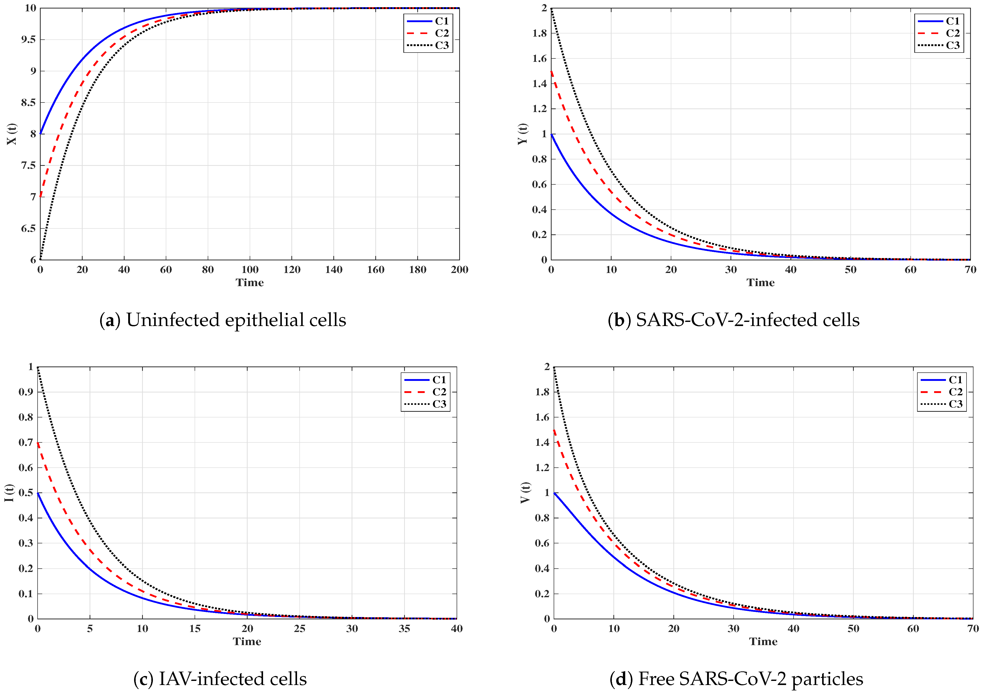
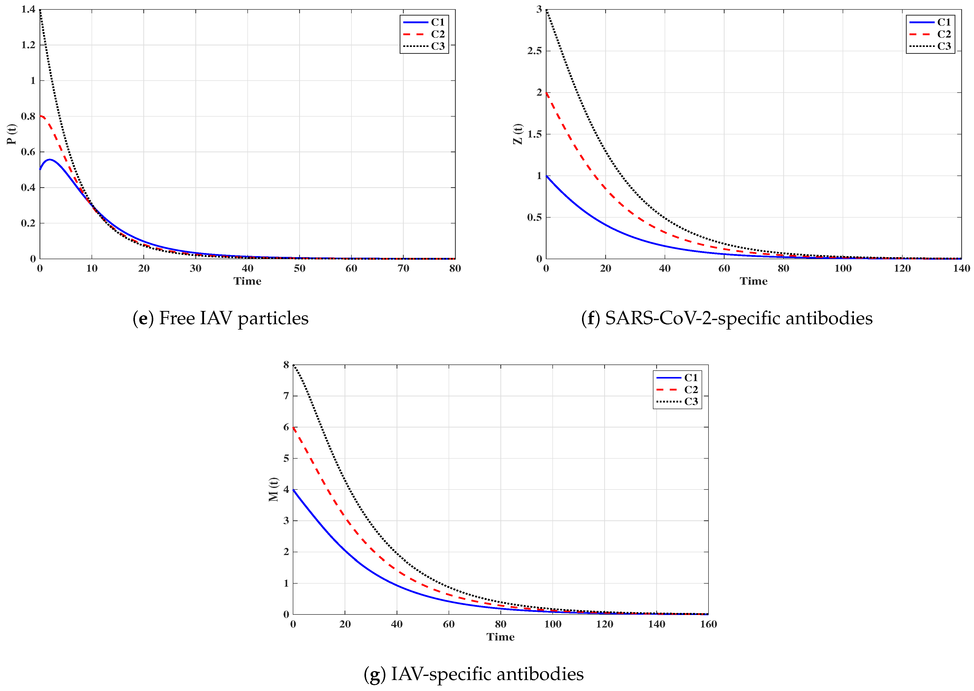
In this subsection, we support our global stability results provided in Theorems 1–8 by showing that the solutions of system (3) with any chosen initial conditions (any IAV/SARS-CoV-2 coinfection stage) will tend to one of the eight equilibria. Let us solve system (3) with three different initial conditions (states) as:

$$\begin{array}{cc}\hfill \mathrm{C}1& :\left(X\right(0),Y(0),I(0),V(0),P(0),Z(0),M(0\left)\right)=(8,1,0.5,1,0.5,1,4),\hfill \\ \hfill \mathrm{C}2& :\left(X\right(0),Y(0),I(0),V(0),P(0),Z(0),M(0\left)\right)=(7,1.5,0.7,1.5,0.8,2,6),\hfill \\ \hfill \mathrm{C}3& :\left(X\right(0),Y(0),I(0),V(0),P(0),Z(0),M(0\left)\right)=(6,2,1,2,1.4,3,8).\hfill \end{array}$$

Selecting the values of ${\beta }_V$,${\beta }_P$,${\sigma }_Z$ and ${\sigma }_M$ leads to the following situations:

Situation 1 (Stability of ${\Xi }_0$):${\beta }_V=0.001,$${\beta }_P=0.001$,${\sigma }_Z=0.01$ and ${\sigma }_M=0.02$. For these values of parameters, we have ${\Re }_1=0.0909<1$ and ${\Re }_2=0.2<1$. Figure 2 shows that the trajectories tend to the equilibrium ${\Xi }_0=(10,0,0,0,0,0,0)$ for all initials C1–C3. This demonstrates that ${\Xi }_0$ is G.A.S. based on Theorem 1. In this situation, both SARS-CoV-2 and IAV will be removed.

Situation 2 (Stability of ${\Xi }_1$):${\beta }_V=0.02,$${\beta }_P=0.001,$${\sigma }_Z=0.002$ and ${\sigma }_M=0.02$. With such selection, we obtain ${\Re }_2=0.2<1<1.8182={\Re }_1$, ${\Re }_3=0.1653<1$ and hence ${\Re }_2/{\Re }_1=0.11<1$. The equilibrium point ${\Xi }_1$ exists with ${\Xi }_1=(5.5,2.05,0,2.05,0,0,0)$. It is clear from Figure 3 that the trajectories tend to ${\Xi }_1$ for all initials. Thus, the numerical results agree with Theorem 2. This case simulates a SARS-CoV-2 single-infection without antibody immunity. In this case, viral interference phenomenon appears, where the SARS-CoV-2 may be able to block the IAV infection.

Situation 3 (Stability of ${\Xi }_2$):${\beta }_V=0.005,$${\beta }_P=0.01$,${\sigma }_Z=0.01$ and ${\sigma }_M=0.005$. This gives ${\Re }_1=0.4545<1<2={\Re }_2$, ${\Re }_4=0.7692<1$ and then ${\Re }_1/{\Re }_2=0.2273<1$. The numerical results show that ${\Xi }_2=\left(5,0,1.25,0,5,0,0\right)$ exists. We can observe from Figure 4 that the trajectories converge to ${\Xi }_2$ regardless of the initial states C1–C3. This result supports the result of Theorem 3. This situation represents an IAV single-infection without antibody immunity. As a result of competition between the two viruses, IAV may be able to block the SARS-CoV-2 infection.

Situation 4 (Stability of ${\Xi }_3$):${\beta }_V=0.02,$${\beta }_P=0.002$,${\sigma }_Z=0.05$ and ${\sigma }_M=0.05$. This yields ${\Re }_3=1.2987>1$ and ${\Re }_5=0.2857<1$. Figure 5 shows that the trajectories tend to ${\Xi }_3=(7.14,1.3,0,1,0,1.19,0)$ regardless of the initial stats C1–C3. Therefore, ${\Xi }_3$ is G.A.S, and this supports Theorem 4. Hence, a SARS-CoV-2 single-infection with stimulated SARS-CoV-2-specific antibody is attained. Despite the activity of antibodies against the SARS-CoV-2 particles, the SARS-CoV-2 may be able to suppress the growth of IAV and block it.

Situation 5 (Stability of ${\Xi }_4$):${\beta }_V=0.01,$${\beta }_P=0.05$,${\sigma }_Z=0.01$ and ${\sigma }_M=0.05$. The values of ${\Re }_4$ and ${\Re }_6$ are computed as ${\Re }_4=5.5556>1$ and ${\Re }_6=0.5051<1$. Thus, ${\Xi }_4$ exists with ${\Xi }_4=(5.56,0,1.11,0,0.8,0,11.39)$. In Figure 6, we see that the trajectories tend to ${\Xi }_4$ regardless of the initial states C1–C3. It follows that ${\Xi }_4$ is G.A.S. according to Theorem 5. Hence, an IAV single-infection with activated IAV-specific antibody is achieved. Despite the activity of antibodies against the IAV particles, the IAV may be able to block the SARS-CoV-2 infection.

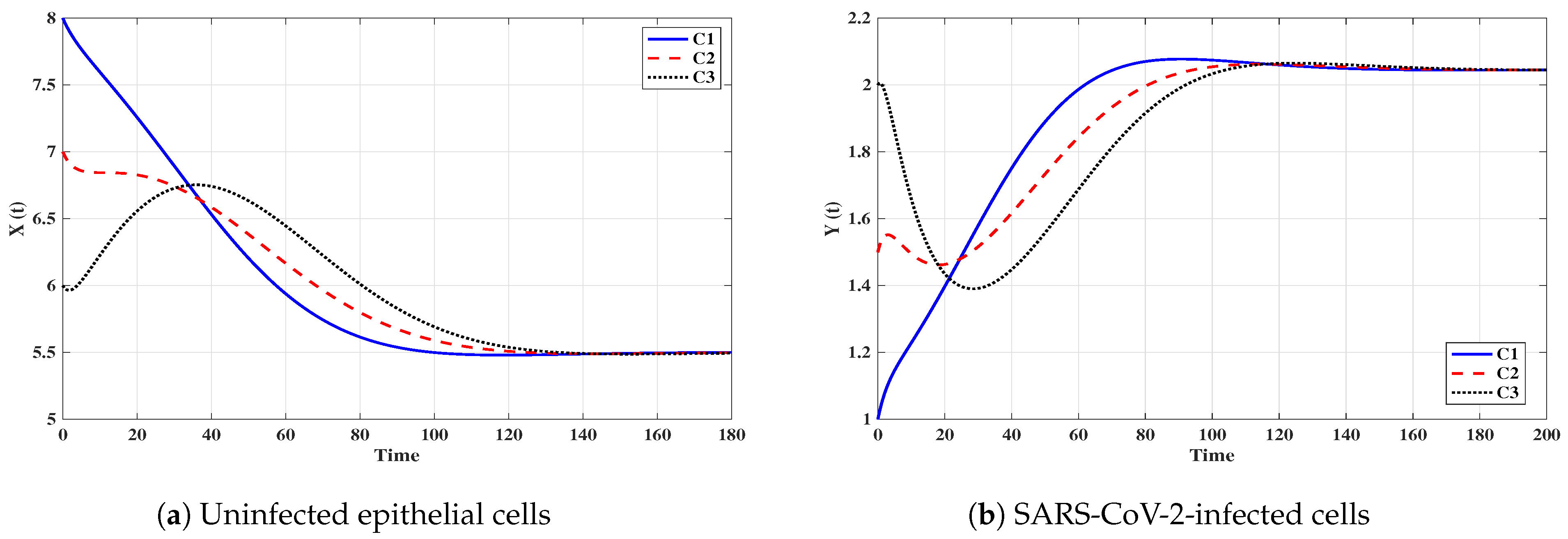
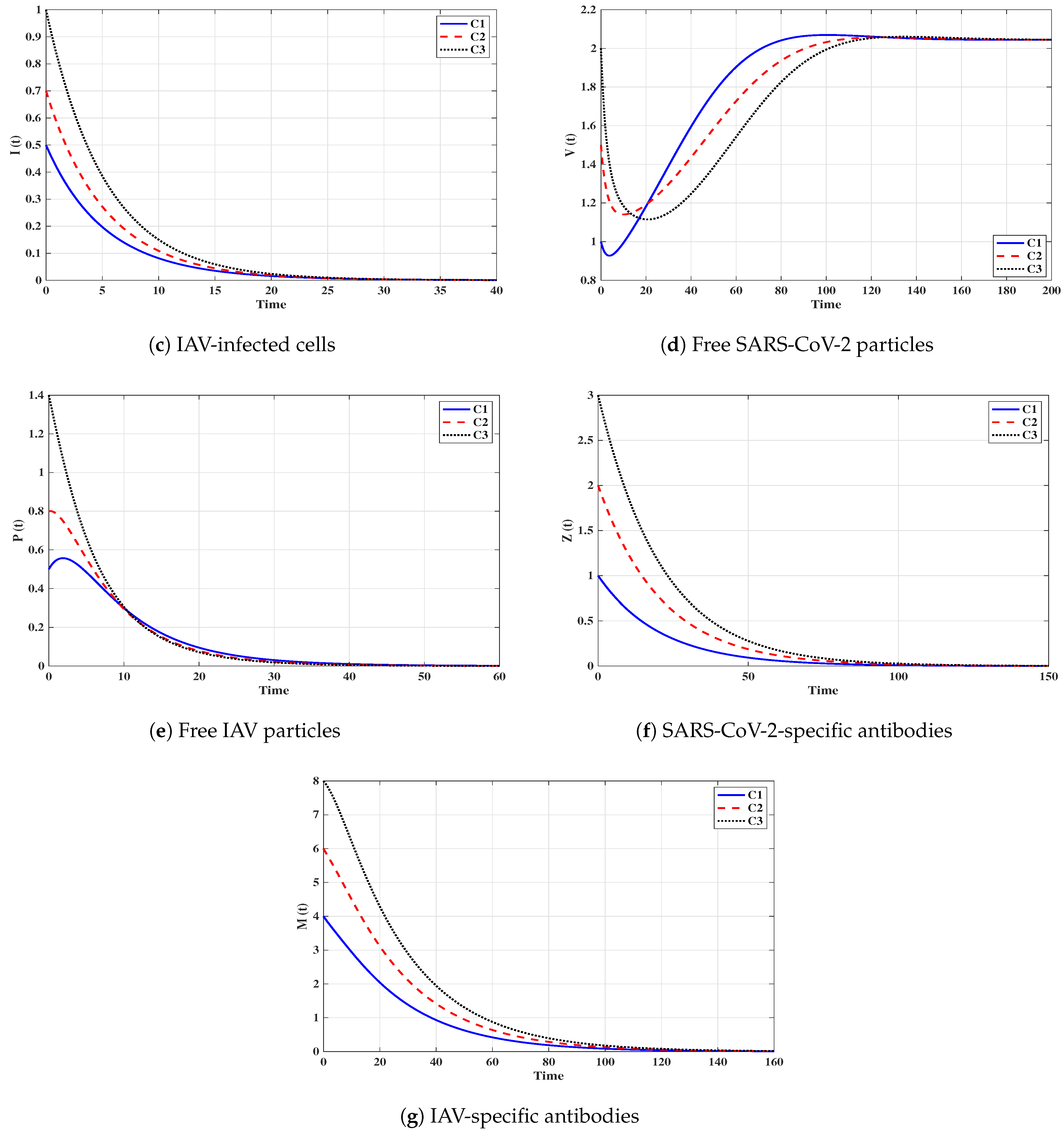
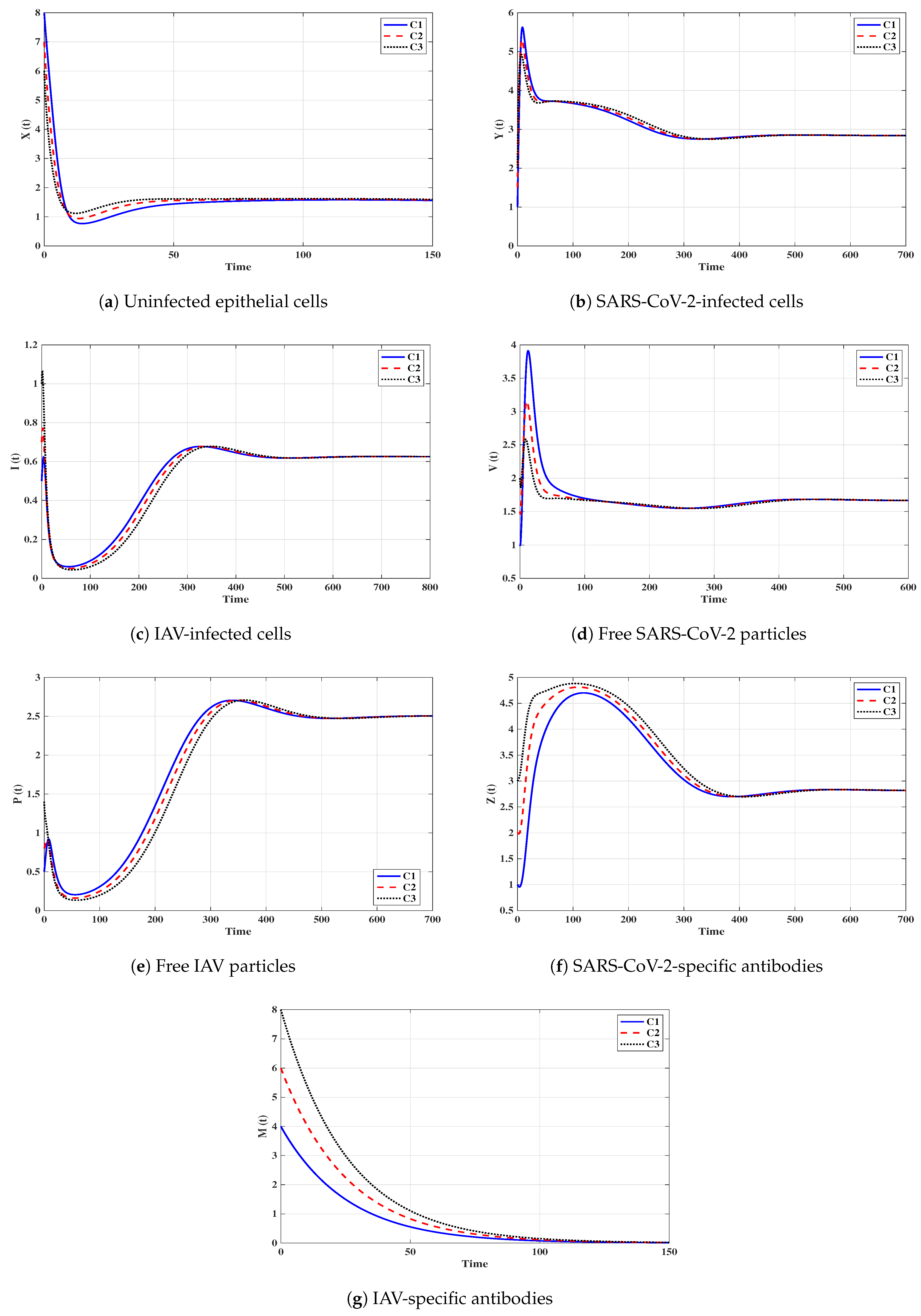
Situation 6 (Stability of ${\Xi }_5$):${\beta }_V=0.15,$${\beta }_P=0.04$,${\sigma }_Z=0.03$ and ${\sigma }_M=0.001$. Then, we calculate ${\Re }_5=1.3333>1$, ${\Re }_7=0.2105<1$ and ${\Re }_1/{\Re }_2=1.7045>1$. The numerical results drawn in Figure 7 show that ${\Xi }_5=(1.25,2.84,0.63,1.67,2.5,2.82,0)$ exists andis G.A.S., and this is consistent with Theorem 6. As a result, a coinfection with SARS-CoV-2 and IAV is attained where only SARS-CoV-2-specific antibody is stimulated. In this case, the concentration of the IAV particles tend to a value less than or equal to $\frac{{\mu }_M}{{\sigma }_M}=40$, and then the IAV-specific antibody will be deactivated. On the other hand, the activity of SARS-CoV-2-specific antibodies reduces the replication of SARS-CoV-2, and this leads to the coexistence of the two viruses.

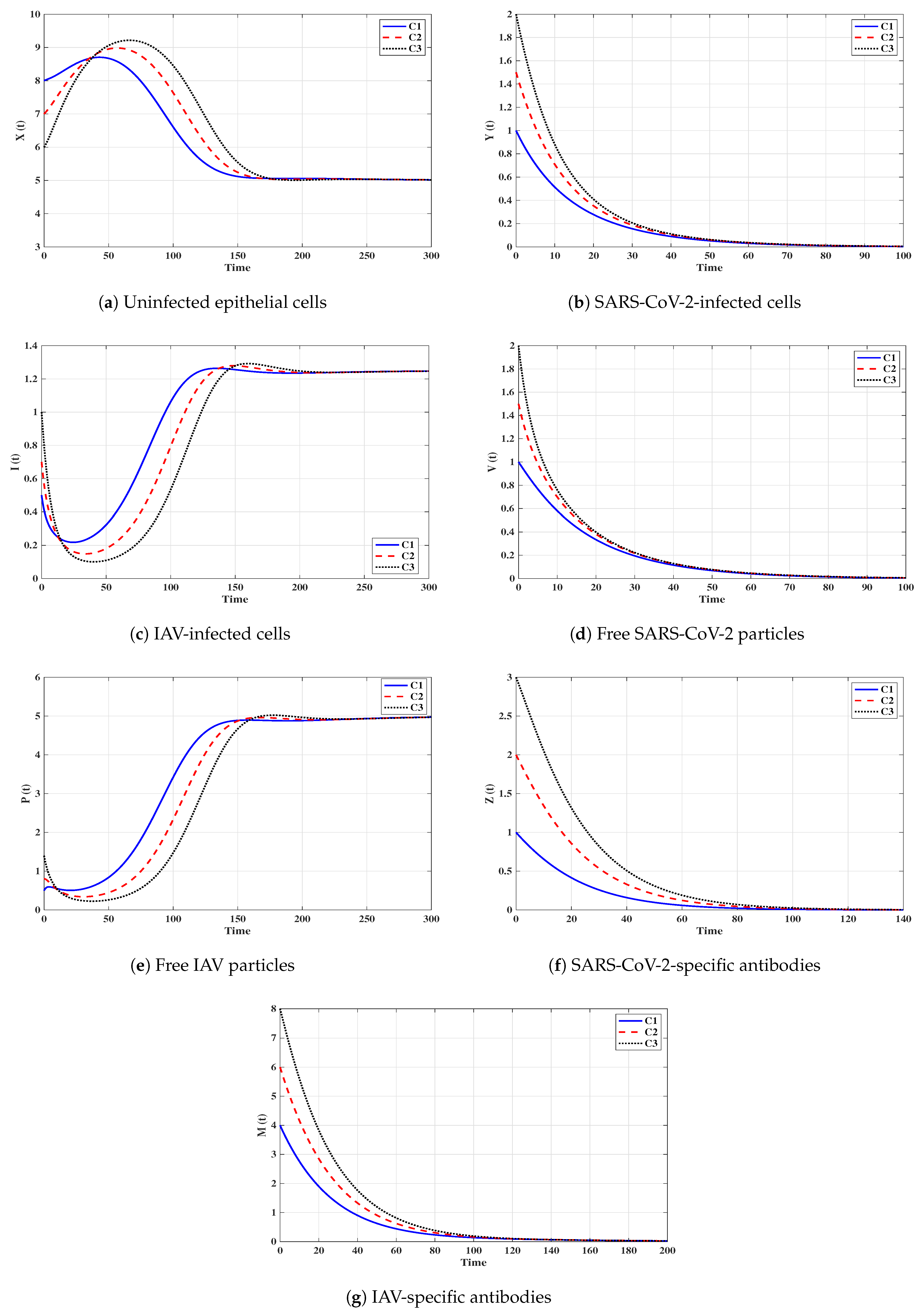
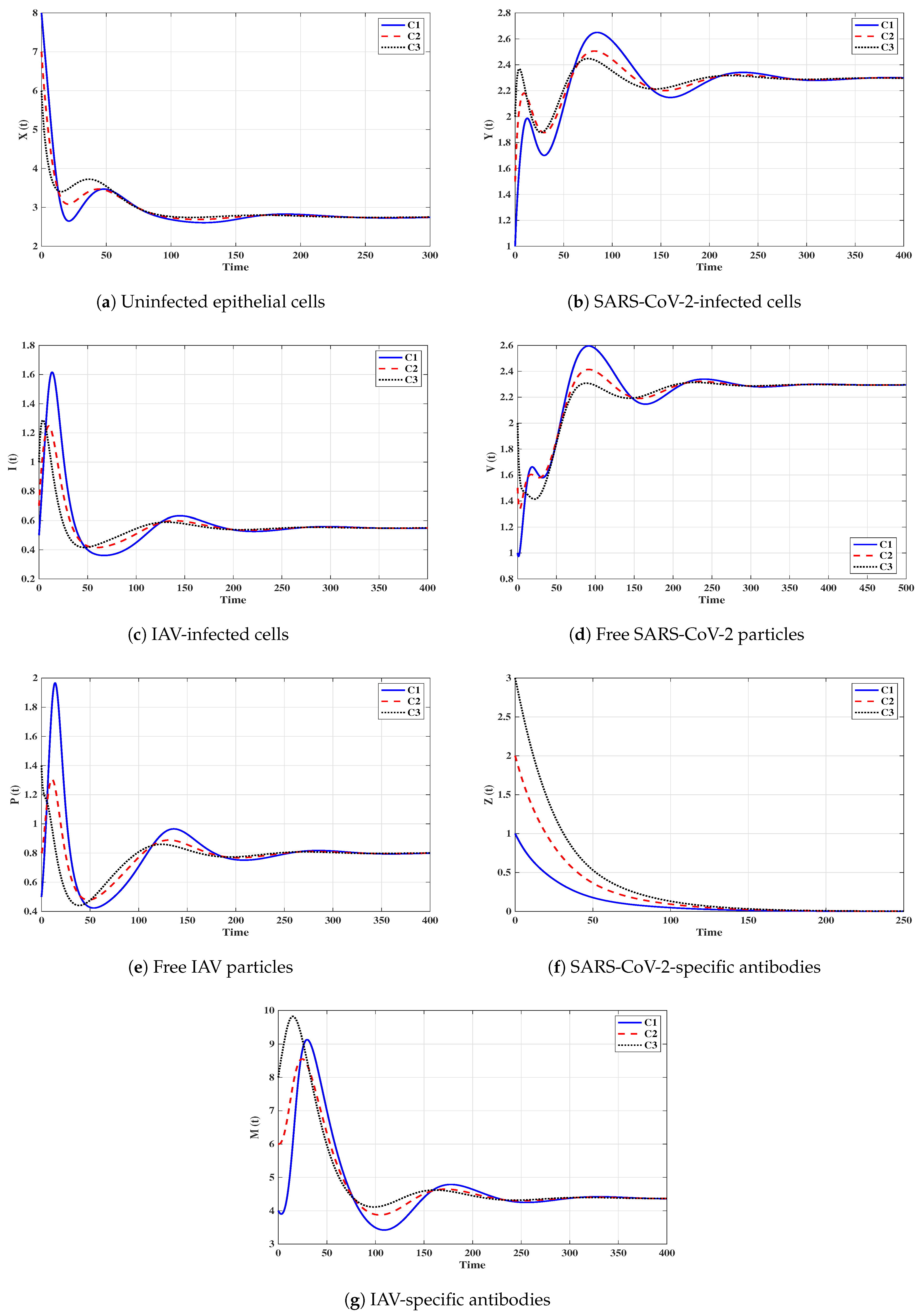
Situation 7 (Stability of ${\Xi }_6$):${\beta }_V=0.04,$${\beta }_P=0.05$,${\sigma }_Z=0.01$ and ${\sigma }_M=0.05$. We compute ${\Re }_6=2.0202>1$, ${\Re }_8=0.627<1$ and ${\Re }_2/{\Re }_1=2.75>1$. We find that the equilibrium ${\Xi }_6=\left(2.75,2.3,0.55,2.3,0.8,0,4.38\right)$ exists. Further, the numerical solutions outlined in Figure 8 show that ${\Xi }_6$ is G.A.S., and this boosts the result of Theorem 7. In this situation, a coinfection with SARS-CoV-2 and IAV is attained where only the IAV-specific antibody is activated. In this case, the concentration of the SARS-CoV-2 particles tends to a value less than or equal to $\frac{{\mu }_Z}{{\sigma }_Z}=5$, and then the SARS-CoV-2-specific antibody will be deactivated. On the other hand, the activity of IAV-specific antibodies reduces the growth of IAV, and this leads to the coexistence of the two viruses.

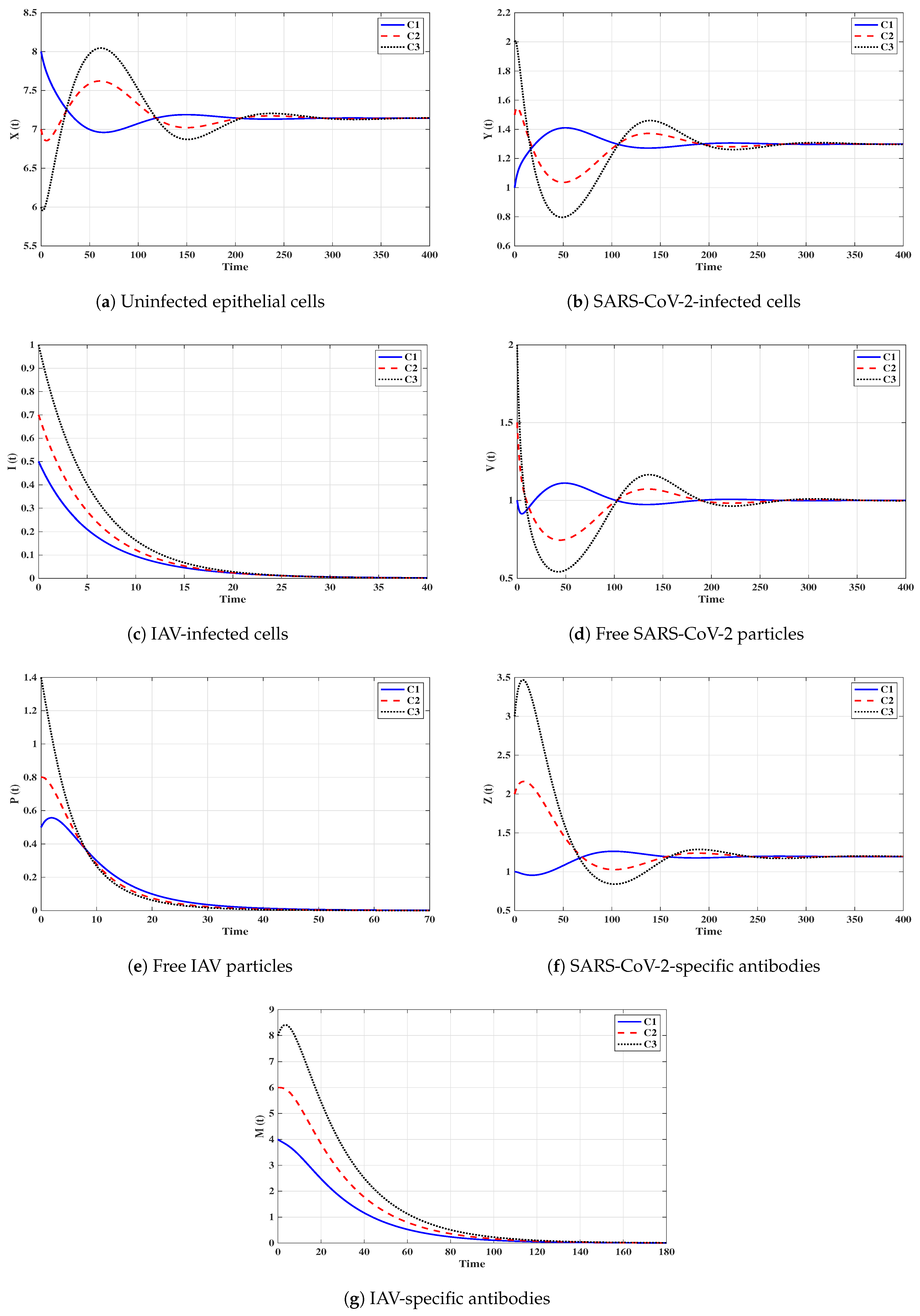
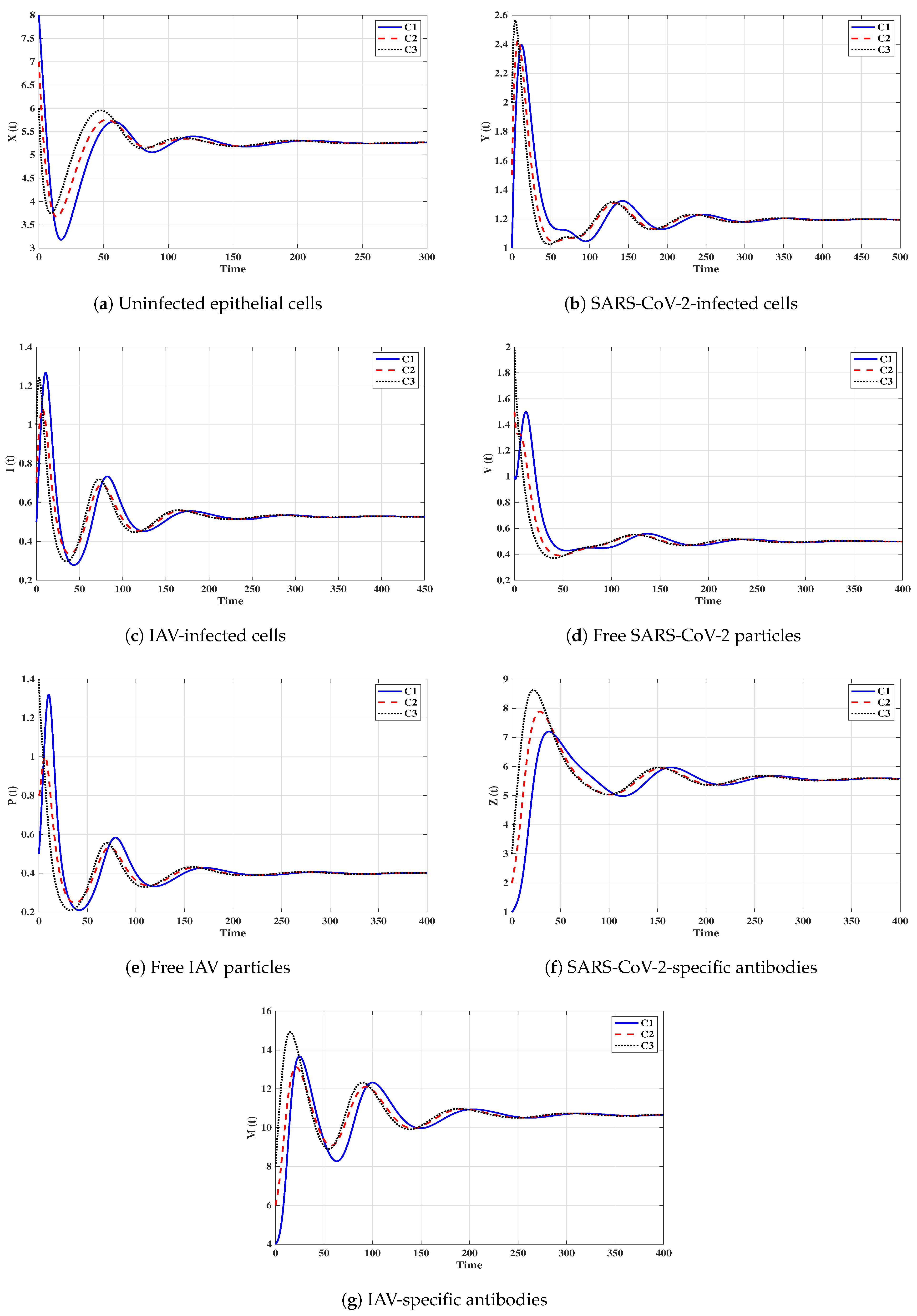
Situation 8 (Stability of ${\Xi }_7$):${\beta }_V=0.05,$${\beta }_P=0.05$,${\sigma }_Z=0.1$ and ${\sigma }_M=0.1$. This selection yields ${\Re }_7=5.2632>1$ and ${\Re }_8=2.3923>1$. Figure 9 shows that ${\Xi }_7=(5.26,1.2,0.53,0.5,0.4,5.57,10.66)$ exists, and it is G.A.S. based on Theorem 8. In this situation, a coinfection with SARS-CoV-2 and IAV is established regardless of the initial states C1–C3. In this case, both SARS-CoV-2-specific antibody and IAV-specific antibody are working against the coinfection. The activation of both SARS-CoV-2-specific and IAV-specific antibodies leads to coexistence of the two viruses.

For more confirmation, we investigate the local stability of the system’s equilibria. Calculating the Jacobian matrix $J=J(X,Y,I,V,P,Z,M)$ of system (3) as:

$$J=\left(\begin{array}{ccccccc}-\left(\alpha +{\beta }_{V}V+{\beta }_{P}P\right)& 0& 0& -{\beta }_{V}X& -{\beta }_{P}X& 0& 0\\ {\beta }_{V}V& -{\gamma }_Y& 0& {\beta }_{V}X& 0& 0& 0\\ {\beta }_{P}P& 0& -{\gamma }_I& 0& {\beta }_{P}X& 0& 0\\ 0& {\kappa }_V& 0& -\left({\pi }_V+{\varkappa }_{V}Z\right)& 0& -{\varkappa }_{V}V& 0\\ 0& 0& {\kappa }_P& 0& -\left({\pi }_P+{\varkappa }_{P}M\right)& 0& -{\varkappa }_{P}P\\ 0& 0& 0& {\sigma }_{Z}Z& 0& {\sigma }_{Z}V-{\mu }_Z& 0\\ 0& 0& 0& 0& {\sigma }_{M}M& 0& {\sigma }_{M}P-{\mu }_M\end{array}\right).$$

(23)

At each equilibrium, we compute the eigenvalues ${\lambda }_j,$$j=1,2,\dots ,7$ of J. If $Re\left({\lambda }_j\right)<0,$$j=1,2,\dots ,7$, then the equilibrium point is locally stable. We select the parameters ${\beta }_V$,${\beta }_P$,${\sigma }_Z$ and ${\sigma }_M$ as given in situations 1–8; then, we compute all nonnegative equilibria and the accompanying eigenvalues.

Table 3. Local stability of nonnegative equilibria ${\Xi }_i$, $i=0,1,\dots ,7$.

Situation	The Equilibria	$Re\left({\mathit{\lambda }}_{\mathit{j}}\right)$$\mathit{j}=1,2,\dots ,7$	Stability
1	$\begin{array}{c}{\Xi }_0=(10,0,0,0,0,0,0)\end{array}$	$\begin{array}{c}\left(-0.23,-0.22,-0.09,-0.07,-0.05,-0.05,-0.04\right)\end{array}$	$\begin{array}{c}\mathrm{stable}\hfill \end{array}$
2	$\begin{array}{c}{\Xi }_0=(10,0,0,0,0,0,0)\hfill \\ {\Xi }_1=(5.5,2.05,0,2.05,0,0,0)\hfill \end{array}$	$\begin{array}{c}\left(-0.36,-0.23,-0.07,-0.05,-0.05,0.05,-0.04\right)\hfill \\ \left(-0.32,-0.22,-0.08,-0.04,-0.04,-0.05,-0.04\right)\hfill \end{array}$	$\begin{array}{c}\mathrm{unstable}\hfill \\ \mathrm{stable}\hfill \end{array}$
3	$\begin{array}{c}{\Xi }_0=(10,0,0,0,0,0,0)\hfill \\ {\Xi }_2=\left(5,0,1.25,0,5,0,0\right)\hfill \end{array}$	$\begin{array}{c}\left(-0.36,-0.26,0.06,-0.05,-0.05,-0.05,-0.04\right)\hfill \\ \left(-0.31,-0.24,-0.07,-0.04,-0.04,-0.05,-0.02\right)\hfill \end{array}$	$\begin{array}{c}\mathrm{unstable}\\ \multicolumn{1}{c}{\mathrm{stable}}\end{array}$
4	$\begin{array}{c}{\Xi }_0=(10,0,0,0,0,0,0)\hfill \\ {\Xi }_1=\left(5.5,2.05,0,2.05,0,0,0\right)\hfill \\ {\Xi }_3=(7.14,1.3,0,1,0,1.19,0)\hfill \end{array}$	$\begin{array}{c}\left(-0.36,-0.25,-0.05,-0.05,0.05,-0.05,-0.04\right)\hfill \\ \left(-0.32,-0.23,-0.07,-0.04,-0.04,0.05,-0.04\right)\hfill \\ \left(-0.37,-0.24,-0.06,-0.04,-0.02,-0.02,-0.04\right)\hfill \end{array}$	$\begin{array}{c}\mathrm{unstable}\\ \mathrm{unstable}\\ \multicolumn{1}{c}{\mathrm{stable}}\end{array}$
5	$\begin{array}{c}{\Xi }_0=(10,0,0,0,0,0,0)\hfill \\ {\Xi }_2=\left(1,0,2.25,0,9,0,0\right)\hfill \\ {\Xi }_4=(5.56,0,1.11,0,0.8,0,11.39)\hfill \end{array}$	$\begin{array}{c}\left(-0.6,-0.3,0.3,-0.05,-0.05,-0.04,-0.007\right)\hfill \\ \left(-0.56,0.41,-0.22,-0.12,-0.12,-0.09,-0.05\right)\hfill \\ \left(-0.75,-0.27,-0.03,-0.03,-0.05,-0.04,-0.04\right)\hfill \end{array}$	$\begin{array}{c}\mathrm{unstable}\\ \mathrm{unstable}\\ \multicolumn{1}{c}{\mathrm{stable}}\end{array}$
6	$\begin{array}{c}{\Xi }_0=(10,0,0,0,0,0,0)\hfill \\ {\Xi }_1=\left(0.73,4.21,0,4.21,0,0,0\right)\hfill \\ {\Xi }_2=\left(1.25,0,2.19,0,8.75,0,0\right)\hfill \\ {\Xi }_3=\left(1.67,3.79,0,1.67,0,5.09,0\right)\hfill \\ {\Xi }_5=(1.25,2.84,0.63,1.67,2.5,2.82,0)\hfill \end{array}$	$\begin{array}{c}\left(-0.7,-0.56,0.39,0.25,-0.05,-0.05,-0.04\right)\hfill \\ \left(-0.73,-0.27,-0.14,-0.14,0.08,-0.04,-0.03\right)\hfill \\ \left(-0.48,-0.35,-0.11,-0.11,-0.05,0.04,-0.03\right)\hfill \\ \left(-0.61,-0.32,-0.11,-0.11,-0.04,-0.03,0.02\right)\hfill \\ \left(-0.56,-0.33,-0.12,-0.12,-0.03,-0.01,-0.01\right)\hfill \end{array}$	$\begin{array}{c}\mathrm{unstable}\\ \mathrm{unstable}\\ \mathrm{unstable}\\ \multicolumn{1}{c}{\mathrm{unstable}}\\ \multicolumn{1}{c}{\mathrm{stable}}\end{array}$
7	$\begin{array}{c}{\Xi }_0=(10,0,0,0,0,0,0)\hfill \\ {\Xi }_1=\left(2.75,3.3,0,3.3,0,0,0\right)\hfill \\ {\Xi }_2=\left(1,0,2.25,0,9,0,0\right)\hfill \\ {\Xi }_4=\left(5.56,0,1.11,0,0.8,0,11.39\right)\hfill \\ {\Xi }_6=\left(2.75,2.3,0.55,2.3,0.8,0,4.38\right)\hfill \end{array}$	$\begin{array}{c}\left(-0.6,-0.4,0.3,0.13,-0.05,-0.05,-0.04\right)\hfill \\ \left(-0.39,-0.36,-0.07,-0.07,0.09,-0.04,-0.02\right)\hfill \\ \left(-0.56,0.41,-0.26,-0.12,-0.12,-0.05,-0.05\right)\hfill \\ \left(-0.75,-0.37,-0.03,-0.03,0.06,-0.05,-0.04\right)\hfill \\ \left(-0.49,-0.34,-0.06,-0.06,-0.01,-0.01,-0.03\right)\hfill \end{array}$	$\begin{array}{c}\mathrm{unstable}\\ \mathrm{unstable}\\ \multicolumn{1}{c}{\mathrm{unstable}}\\ \mathrm{unstable}\\ \multicolumn{1}{c}{\mathrm{stable}}\end{array}$
8	$\begin{array}{c}{\Xi }_0=(10,0,0,0,0,0,0)\hfill \\ {\Xi }_1=\left(2.2,3.55,0,3.55,0,0,0\right)\hfill \\ {\Xi }_2=\left(1,0,2.25,0,9,0,0\right)\hfill \\ {\Xi }_3=\left(6.67,1.52,0,0.5,0,8.12,0\right)\hfill \\ {\Xi }_4=\left(7.14,0,0.71,0,0.4,0,15.36\right)\hfill \\ {\Xi }_6=\left(2.2,3.15,0.22,3.15,0.4,0,3\right)\hfill \\ {\Xi }_7=\left(5.26,1.2,0.53,0.5,0.4,5.57,10.66\right)\hfill \end{array}$	$\begin{array}{c}\left(-0.6,-0.47,0.3,0.16,-0.05,-0.05,-0.04\right)\hfill \\ \left(-0.38,-0.37,0.31,-0.08,-0.08,-0.07,-0.04\right)\hfill \\ \left(0.86,-0.56,-0.26,-0.12,-0.12,-0.05,-0.05\right)\hfill \\ \left(-0.7,-0.52,0.22,-0.02,-0.02,-0.05,-0.04\right)\hfill \\ \left(-0.9,-0.43,0.12,-0.02,-0.02,-0.05,-0.05\right)\hfill \\ \left(-0.43,-0.36,0.27,-0.08,-0.08,-0.006,-0.006\right)\hfill \\ \left(-0.71,-0.57,-0.03,-0.03,-0.02,-0.02,-0.04\right)\hfill \end{array}$	$\begin{array}{c}\mathrm{unstable}\\ \mathrm{unstable}\\ \mathrm{unstable}\\ \multicolumn{1}{c}{\mathrm{unstable}}\\ \mathrm{unstable}\\ \mathrm{unstable}\\ \multicolumn{1}{c}{\mathrm{stable}}\end{array}$

outlined the nonnegative equilibria, the real parts of the eigenvalues and whether or not the equilibrium point is stable. We found that the local stability agrees with the global one.

6.2. Comparison Results

In this subsection, we present a comparison between the single-infection and coinfection.

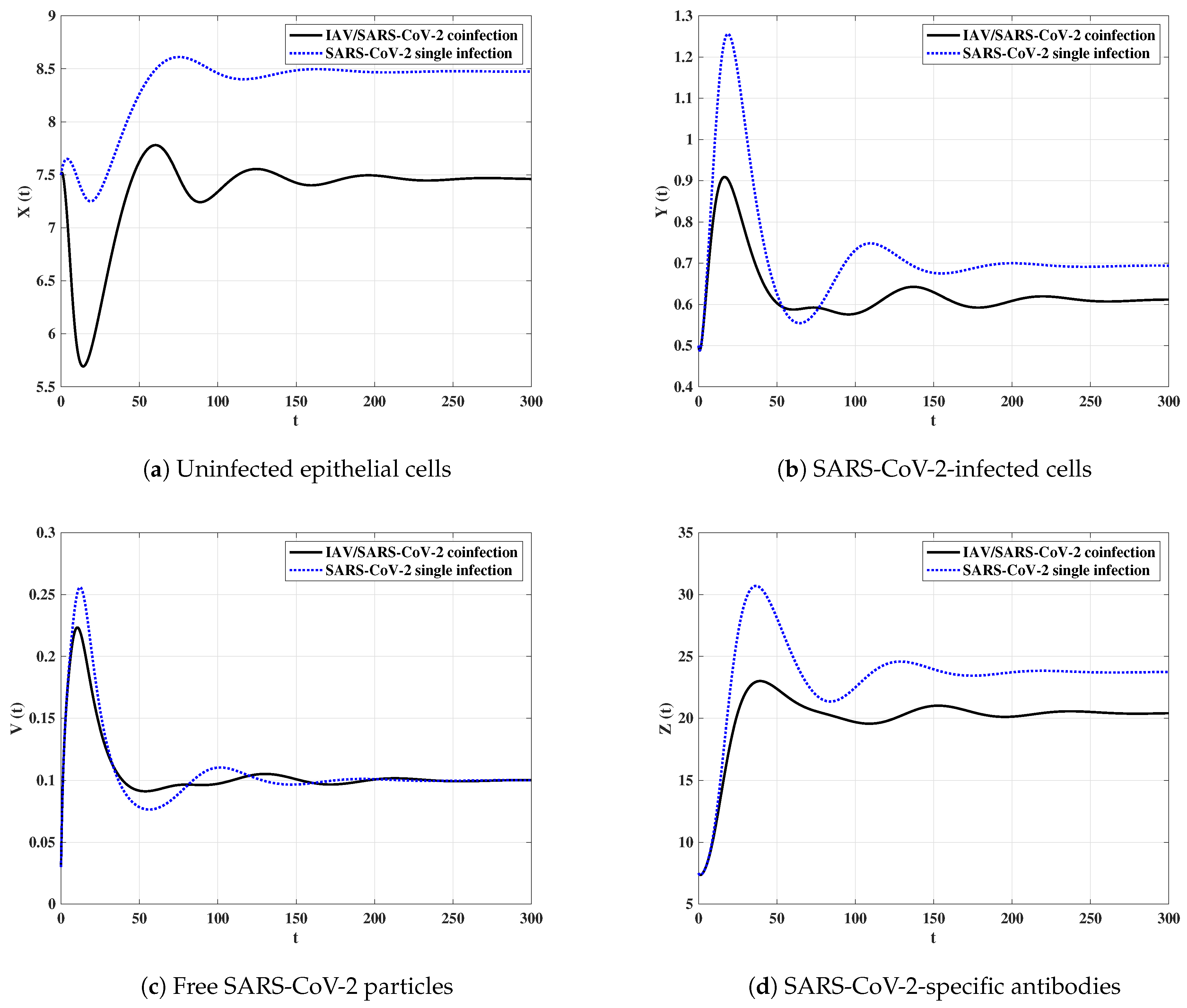
Influence of IAV infection on the dynamics of SARS-CoV-2 single-infection

Here, we compare the solutions of model (3) and the following SARS-CoV-2 single-infection model:

$$\left\{\begin{array}{c}\dot{X}=\lambda -\alpha X-{\beta }_{V}XV,\hfill \\ \dot{Y}={\beta }_{V}XV-{\gamma }_{Y}Y,\hfill \\ \dot{V}={\kappa }_{V}Y-{\pi }_{V}V-{\varkappa }_{V}VZ,\hfill \\ \dot{Z}={\sigma }_{Z}VZ-{\mu }_{Z}Z.\hfill \end{array}\right.$$

(24)

We fix parameters ${\beta }_V=0.09$, ${\beta }_P=0.05$, ${\sigma }_Z=0.5$ and ${\sigma }_M=0.9$ and select the initial state as:

$$\mathrm{C}4:(X\left(0\right),Y\left(0\right),I\left(0\right),V\left(0\right),P\left(0\right),Z\left(0\right),M\left(0\right))=\left(7.5,0.5,0.4,0.03,0.04,7.5,9.5\right)$$

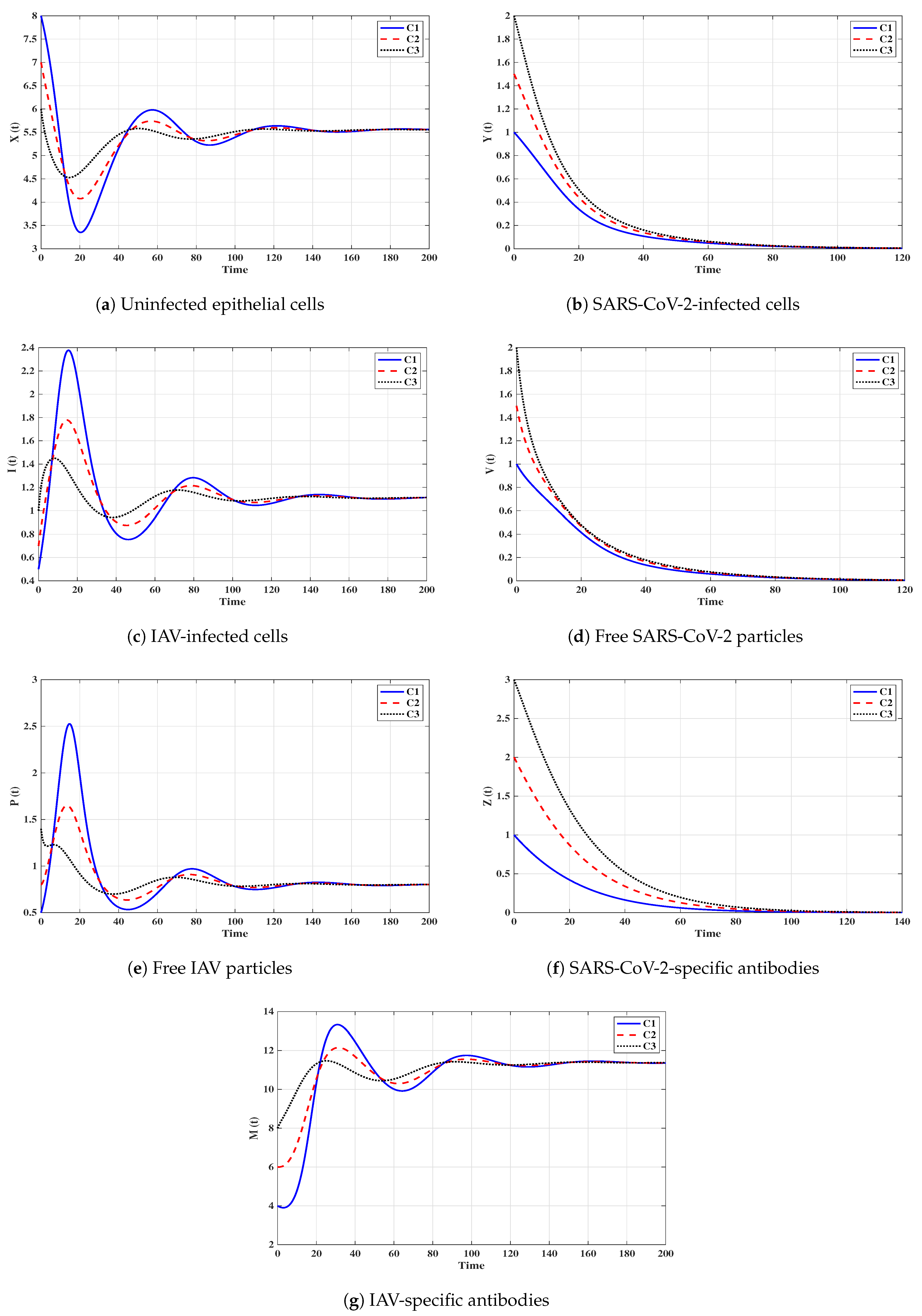
From Figure 10, we observe that when the SARS-CoV-2 single-infected individual is coinfected with IAV, then the concentrations of uninfected epithelial cells, SARS-CoV-2-infected cells and SARS-CoV-2-specific antibodies are reduced. However, the concentration of free SARS-CoV-2 particles tend to be the same value in both SARS-CoV-2 single-infection and IAV/SARS-CoV-2 coinfection. This result agrees with the observation of Ding et al. [10] which said that “IAV/SARS-CoV-2 coinfection did not result in worse clinical outcomes in comparison with SARS-CoV-2 single-infection”.

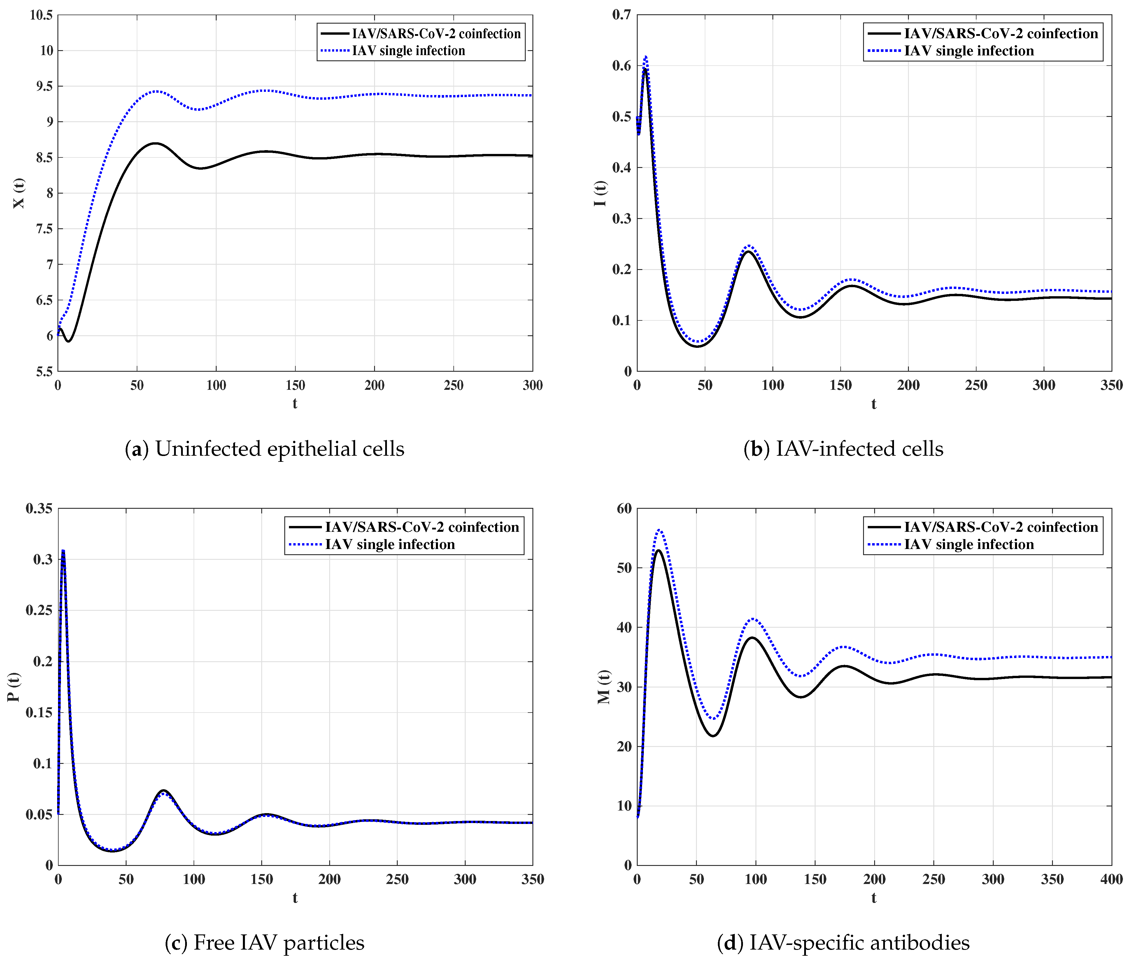
Influence of SARS-CoV-2 infection on the dynamics of IAV single-infection

To examine the impact of SARS-CoV-2 infection on IAV single-infection, we compare the solutions of model (3) and the following IAV single-infection model:

$$\left\{\begin{array}{c}\dot{X}=\lambda -\alpha X-{\beta }_{P}XP,\hfill \\ \dot{I}={\beta }_{P}XP-{\gamma }_{I}I,\hfill \\ \dot{P}={\kappa }_{P}I-{\pi }_{P}P-{\varkappa }_{P}PM,\hfill \\ \dot{M}={\sigma }_{M}PM-{\mu }_{M}M.\hfill \end{array}\right.$$

(25)

We fix parameters ${\beta }_V=$$0.095$, ${\beta }_P=0.08$, ${\sigma }_Z=0.9$ and ${\sigma }_M=0.95$ and consider the following initial condition:

$$\mathrm{C}5:(X\left(0\right),Y\left(0\right),I\left(0\right),V\left(0\right),P\left(0\right),Z\left(0\right),M\left(0\right))=\left(6,0.6,0.5,0.05,0.05,7.05,8.05\right).$$

It can be observed from Figure 11 that when the IAV single-infected individual is coinfected with SARS-CoV-2, then the concentrations of uninfected epithelial cells, IAV-infected cells and IAV-specific antibodies are decreased. However, the concentration of free IAV particles cells tends to the same value in both IAV single-infection and IAV/SARS-CoV-2 coinfection.

7. Discussion

IAV and SARS-CoV-2 coinfection cases were reported in some works (see [1,8,10,11]). Therefore, it is important to understand the within-host dynamics of this coinfection. In this paper, we develop and examine a within-host IAV/SARS-CoV-2 coinfection model. We studied the basic and global properties of the model. We find that the system has eight equilibria, and their existence and global stability are governed by eight threshold parameters (${\Re }_i$, $i=1,\dots ,8$). We proved the following:

(I) The infection-free equilibrium ${\Xi }_0$ always exists. It is G.A.S. when ${\Re }_1\le 1$ and ${\Re }_2\le 1$. In this case, the patient is recovered from both IAV and SARS-CoV-2 infections. From a control viewpoint, making ${\Re }_1\le 1$ and ${\Re }_2\le 1$ will be a good strategy. This can be achieved by reducing the parameters ${\beta }_V$ and ${\beta }_P$ (or ${\kappa }_V$ and ${\kappa }_P$). Let ${ϵ}_V\in [0,1]$ and ${ϵ}_P\in [0,1]$ be the effectiveness of the antiviral drugs for SARS-CoV-2 and IAV, respectively. Then, the parameters ${\beta }_V$ and ${\beta }_P$ will be changed to $(1-{ϵ}_V){\beta }_V$ and $(1-{ϵ}_P){\beta }_P$. Moreover, ${\Re }_1$ and ${\Re }_2$ become

$${\Re }_1\left({ϵ}_V\right)=\frac{(1-{ϵ}_V)X_0{\kappa }_V{\beta }_V}{{\pi }_V{\gamma }_Y},{\Re }_2\left({ϵ}_P\right)=\frac{(1-{ϵ}_P)X_0{\kappa }_P{\beta }_P}{{\pi }_P{\gamma }_I}.$$

To make ${\Re }_1\le 1$ and ${\Re }_2\le 1$, the effectiveness ${ϵ}_V$ and ${ϵ}_P$ have to satisfy

$$\begin{array}{cc}\hfill {ϵ}_V^{min}& \le {ϵ}_V\le 1,{ϵ}_V^{min}=max\left\{0,1-\frac{1}{{\Re }_1\left(0\right)}\right\},\hfill \\ \hfill {ϵ}_P^{min}& \le {ϵ}_P\le 1,{ϵ}_P^{min}=max\left\{0,1-\frac{1}{{\Re }_2\left(0\right)}\right\}.\hfill \end{array}$$

(II) The SARS-CoV-2 single-infection equilibrium without antibody immunity ${\Xi }_1$ exists if ${\Re }_1>1$. It is G.A.S. when ${\Re }_1>1$, ${\Re }_2/{\Re }_1\le 1$ and ${\Re }_3\le 1$. This case leads to the situation of a patient who is only infected by SARS-CoV-2 with inactive immune response. As we will see below, if both SARS-CoV-2-specific antibody and IAV-specific antibody immunities are not activated against the two viruses, then according to the competition between the two viruses, SARS-CoV-2 may be able to block the IAV infection.

(III) The IAV single-infection equilibrium without antibody immunity ${\Xi }_2$ exists if ${\Re }_2>1$. It is G.A.S. when ${\Re }_2>1$, ${\Re }_1/{\Re }_2\le 1$ and ${\Re }_4\le 1$. This case leads to the situation of a patient who is only infected by IAV with unstimulated immune response. Then, IAV may be able to block the SARS-CoV-2 infection.

(IV) The SARS-CoV-2 single-infection equilibrium with stimulated SARS-CoV-2-specific antibody immunity ${\Xi }_3$ exists if ${\Re }_3>1$. It is G.A.S. when ${\Re }_3>1$ and ${\Re }_5\le 1$. This point represents the situation of a SARS-CoV-2 single-infection patient with active SARS-CoV-2-specific antibody immunity. Despite the activity of antibodies against the SARS-CoV-2 particles, the SARS-CoV-2 may be able to block the IAV.

(V) The IAV single-infection equilibrium with stimulated IAV-specific antibody immunity ${\Xi }_4$ exists if ${\Re }_4>1$. It is G.A.S. when ${\Re }_4>1$ and ${\Re }_6\le 1$. This point represents the case of an IAV single-infection patient with active IAV-specific antibody immunity. Despite the activity of antibodies against the IAV particles, the IAV may be able to block the SARS-CoV-2.

(VI) The IAV/SARS-CoV-2 coinfection equilibrium with only stimulated SARS-CoV-2-specific antibody immunity ${\Xi }_5$ exists if ${\Re }_5>1$ and ${\Re }_1/{\Re }_2>1$. It is G.A.S. when ${\Re }_5>1$, ${\Re }_7\le 1$ and ${\Re }_1/{\Re }_2>1$. Here, the IAV/SARS-CoV-2 coinfection occurs with only stimulated SARS-CoV-2-specific antibody immunity. The activity of SARS-CoV-2-specific antibodies suppresses the growth of SARS-CoV-2 particles, and this makes IAV coexist with SARS-CoV-2.

(VII) The IAV/SARS-CoV-2 coinfection equilibrium with only stimulated IAV-specific antibody immunity ${\Xi }_6$ exists if ${\Re }_6>1$ and ${\Re }_2/{\Re }_1>1$. It is G.A.S. when ${\Re }_6>1$, ${\Re }_8\le 1$ and ${\Re }_2/{\Re }_1>1$. It means that the IAV/SARS-CoV-2 coinfection occurs with only stimulated IAV-specific antibody immunity. The activity of IAV-specific antibodies reduces the replication of IAV particles, and this makes SARS-CoV-2 coexist with IAV.

(VIII) The IAV/SARS-CoV-2 coinfection equilibrium with both stimulated SARS-CoV-2-specific antibody and IAV-specific antibody immunities ${\Xi }_7$ exists, and it is G.A.S. when ${\Re }_7>1$ and ${\Re }_8>1$. It means that the IAV/SARS-CoV-2 coinfection occurs with both SARS-CoV-2-specific antibody and IAV-specific antibody immunities activated. Since both SARS-CoV-2-specific and IAV-specific antibodies are activated, then coexistence of the two viruses appears.

We discussed the influence of IAV infection on SARS-CoV-2 single-infection dynamics and vice versa. We found that the concentration of free IAV or SARS-CoV-2 particles cells tend to be the same value in both single-infection and coinfection. This agrees with the work Ding et al. [10] which reported that IAV/SARS-CoV-2 coinfection did not result in worse clinical outcomes [10]. In addition, the spread of seasonal influenza can increase the likelihood of coinfection in patients with COVID-19 [8].

From the above, we note that the coexistence case of IAV and SARS-CoV-2 can occur if at least one type of the specific antibody immunity is active. Now, we discuss the importance of considering the antibody immune response in the IAV/SARS-CoV-2 dynamics model. If the antibody immune response is neglected, then system (3) becomes:

$$\left\{\begin{array}{c}\dot{X}=\lambda -\alpha X-{\beta }_{V}XV-{\beta }_{P}XP,\hfill \\ \dot{Y}={\beta }_{V}XV-{\gamma }_{Y}Y,\hfill \\ \dot{I}={\beta }_{P}XP-{\gamma }_{I}I,\hfill \\ \dot{V}={\kappa }_{V}Y-{\pi }_{V}V,\hfill \\ \dot{P}={\kappa }_{P}I-{\pi }_{P}P.\hfill \end{array}\right.$$

(26)

We can see that system (26) describes the competition between IAV and SARS-CoV-2 on one source of target cells, epithelial cells. The model admits only three equilibria:

(i) Infection-free equilibrium, ${\tilde{\Xi }}_0=({\tilde{X}}_0,0,0,0,0)$, where both IAV and SARS-CoV-2 are cleared,

(ii) SARS-CoV-2 single-infection equilibrium ${\tilde{\Xi }}_1=({\tilde{X}}_1,{\tilde{Y}}_1,0,{\tilde{V}}_1,0)$, where the IAV is blocked,

(iii) IAV single-infection equilibrium, ${\tilde{\Xi }}_2=({\tilde{X}}_2,0,{\tilde{I}}_2,0,{\tilde{P}}_2)$, where the SARS-CoV-2 is blocked, where ${\tilde{X}}_i=X_i$, $i=0,1,2$, ${\tilde{Y}}_1=Y_1$, ${\tilde{V}}_1=V_1$, ${\tilde{I}}_2=I_2,$ and ${\tilde{P}}_2=P_2$.

We note that the case of IAV and SARS-CoV-2 coexistence does not appear. In the recent studies presented in [1,8,10,11], it was recorded that some COVID-19 patients were coinfected with IAV. Therefore, neglecting the immune response may not describe the coinfection dynamics accurately. This supports the idea of including the immune response into the IAV/SARS-CoV-2 coinfection model, where the case of IAV and SARS-CoV-2 coexistence is observed.

8. Conclusions

Mathematical models are frequently used to understand the complex behavior of biological systems. In this paper, we formulated an IAV and SARS-CoV-2 coinfection model within a host. The model is a seven-dimensional nonlinear ODEs which describes the interaction between uninfected epithelial cells, SARS-CoV-2-infected cells, IAV-infected cells, free SARS-CoV-2 particles, free IAV particles, SARS-CoV-2-specific antibodies and IAV-specific antibodies. The regrowth and death of the uninfected epithelial cells are considered. We first examined the nonnegativity and boundedness of the solutions; then we calculated the model’s equilibria and established their existence in terms of eight threshold parameters. We proved the global stability of all equilibria by constructing Lyapunov functions and applying the Lyapunov–LaSalle asymptotic stability theorem. We performed numerical simulations and demonstrated that they are in good agreement with the theoretical results. We discussed the effect of including the antibody immunity into the coinfection dynamics model. We found that including the antibody immunity in the coinfection model plays an important role in establishing the case of IAV and SARS-CoV-2 coexistence which is practically detected in many patients. Finally, we discussed the influence of IAV infection on the dynamics of SARS-CoV-2 single-infection and vice versa.

The model proposed in this research and its analysis shows three main biological states, (i) clearance of both IAV and SARS-CoV-2 particles, (ii) appearance of interference phenomenon, where one virus may be able to suppress the growth of another virus, and (iii) coexistence of the two viruses.

The model developed in this work can be improved by (i) utilizing real data to find a good estimation of the parameters’ values, (ii) studying the effect of time delays that occur during infection or production of IAV and SARS-CoV-2 particles [45], (iii) considering viral mutations [65,66], (iv) considering the effect of treatments on the progression of both viruses, and (v) including the influence of Cytotoxic T-Lymphocytes (CTLs) in killing SARS-CoV-2-infected and IAV-infected cells [40]. These research points need further investigations so we leave them to future works.

References

- Ozaras, R. Influenza and COVID-19 coinfection: Report of six cases and review of the literature. J. Med. Virol. 2020, 92, 2657–2665. [Google Scholar] [CrossRef]
- Coronavirus Disease (COVID-19), Weekly Epidemiological Update, World Health Organization (WHO). 2022. Available online: https://www.who.int/publications/m/item/weekly-epidemiological-update-on-covid-19---24-august-2022 (accessed on 21 August 2022).
- Coronavirus Disease (COVID-19), Vaccine Tracker, World Health Organization (WHO). 2022. Available online: https://covid19.trackvaccines.org/agency/who/ (accessed on 2 October 2022).
- Enomoto, T.; Shiroyama, T.; Hirata, H.; Amiya, S.; Adachi, Y.; Niitsu, T.; Noda, Y.; Hara, R.; Fukushima, K.; Suga, Y.; et al. COVID-19 in a human T-cell lymphotropic virus type-1 carrier. Clin. Case Rep. 2022, 10, e05463. [Google Scholar] [CrossRef]
- Hernez-Vargas, E.A.; Wilk, E.; Canini, L.; Toapanta, F.R.; Binder, S.C.; Uvarovskii, A.; Meyer-Hermann, M. Effects of aging on influenza virus infection dynamics. J. Virol. 2014, 88, 4123–4131. [Google Scholar] [CrossRef] [PubMed] [Green Version]
- Smith, A.M.; Smith, A.P. A critical, nonlinear threshold dictates bacterial invasion and initial kinetics during influenza. Sci. Rep. 2016, 6, 38703. [Google Scholar] [CrossRef] [Green Version]
- Hancioglu, B.; Swigon, D.; Clermont, G. A dynamical model of human immune response to influenza A virus infection. J. Theor. Biol. 2007, 246, 70–86. [Google Scholar] [CrossRef]
- Zhu, X.; Ge, Y.; Wu, T.; Zhao, K.; Chen, Y.; Wu, B.; Cui, L. Co-infection with respiratory pathogens among COVID-2019 cases. Virus Res. 2020, 285, 198005. [Google Scholar] [CrossRef]
- Aghbash, P.S.; Eslami, N.; Shirvaliloo, M.; Baghi, H. Viral coinfections in COVID-19. J. Med Virol. 2021, 93, 5310–5322. [Google Scholar] [CrossRef]
- Ding, Q.; Lu, P.; Fan, Y.; Xia, Y.; Liu, M. The clinical characteristics of pneumonia patients coinfected with 2019 novel coronavirus and influenza virus in Wuhan, China. J. Med Virol. 2020, 92, 1549–1555. [Google Scholar] [CrossRef]
- Wang, G.; Xie, M.; Ma, J.; Guan, J.; Song, Y.; Wen, Y.; Fang, D.; Wang, M.; Tian, D.; Li, P. Is co-Infection with Influenza Virus a Protective Factor of COVID-19? 2020. Available online: https://papers.ssrn.com/sol3/papers.cfm?abstract_id=3576904 (accessed on 2 October 2022).
- Wang, M.; Wu, Q.; Xu, W.; Qiao, B.; Wang, J.; Zheng, H.; Li, Y. Clinical diagnosis of 8274 samples with 2019-novel coronavirus in Wuhan. MedRxiv 2020. [Google Scholar] [CrossRef] [Green Version]
- Lansbury, L.; Lim, B.; Baskaran, V.; Lim, W.S. Co-infections in people with COVID-19: A systematic review and meta-analysis. J. Infect. 2020, 81, 266–275. [Google Scholar] [CrossRef] [PubMed]
- Ghaznavi, H.; Shirvaliloo, M.; Sargazi, S.; Mohammadghasemipour, Z.; Shams, Z.; Hesari, Z.; Shirvalilou, S. SARS-CoV-2 and influenza viruses: Strategies to cope with coinfection and bioinformatics perspective. Cell Biol. Int. 2022, 46, 1009–1020. [Google Scholar] [CrossRef] [PubMed]
- Khorramdelazad, H.; Kazemi, M.H.; Najafi, A.; Keykhaee, M.; Emameh, R.Z.; Falak, R. Immunopathological similarities between COVID-19 and influenza: Investigating the consequences of co-infection. Microb. Pathog. 2021, 152, 104554. [Google Scholar] [CrossRef]
- Xiang, X.; Wang, Z.H.; Ye, L.L.; He, X.L.; Wei, X.S.; Ma, Y.L.; Zhou, Q. Co-infection of SARS-COV-2 and influenza A virus: A case series and fast review. Curr. Med. Sci. 2021, 41, 51–57. [Google Scholar] [CrossRef] [PubMed]
- Nowak, M.D.; Sordillo, E.M.; Gitman, M.R.; Mondolfi, A.E. Coinfection in SARS-CoV-2 infected patients: Where are influenza virus and rhinovirus/enterovirus? J. Med. Virol. 2020, 92, 1699. [Google Scholar] [CrossRef] [PubMed]
- Pinky, L.; Dobrovolny, H.M. SARS-CoV-2 coinfections: Could influenza and the common cold be beneficial? J. Med. Virol. 2020, 92, 2623–2630. [Google Scholar] [CrossRef]
- Pinky, L.; Dobrovolny, H.M. Coinfections of the respiratory tract: Viral competition for resources. PLoS ONE 2016, 11, e0155589. [Google Scholar] [CrossRef] [PubMed]
- Baccam, P.; Beauchemin, C.; Macken, C.A.; Hayden, F.G.; Perelson, A. Kinetics of influenza A virus infection in humans. J. Virol. 2006, 80, 7590–7599. [Google Scholar] [CrossRef] [PubMed] [Green Version]
- Smith, A.M.; Ribeiro, R.M. Modeling the viral dynamics of influenza A virus infection. Crit. Rev. Immunol. 2010, 30, 291–298. [Google Scholar] [CrossRef] [PubMed]
- Beauchemin, C.A.; Handel, A. A review of mathematical models of influenza A infections within a host or cell culture: Lessons learned and challenges ahead. BMC Public Health 2011, 11, 1–15. [Google Scholar] [CrossRef] [Green Version]
- Canini, L.; Perelson, A.S. Viral kinetic modeling: State of the art. J. Pharmacokinet. Pharmacodyn. 2014, 41, 431–443. [Google Scholar] [CrossRef]
- Handel, A.; Liao, L.E.; Beauchemin, C.A. Progress and trends in mathematical modelling of influenza A virus infections. Curr. Opin. Syst. Biol. 2018, 12, 30–36. [Google Scholar] [CrossRef]
- Saenz, R.A.; Quinlivan, M.; Elton, D.; MacRae, S.; Blunden, A.S.; Mumford, J.A.; Gog, J.R. Dynamics of influenza virus infection and pathology. J. Virol. 2010, 84, 3974–3983. [Google Scholar] [CrossRef] [PubMed] [Green Version]
- Lee, H.Y.; Topham, D.J.; Park, S.Y.; Hollenbaugh, J.; Treanor, J.; Mosmann, T.R.; Jin, X.; Ward, B.M.; Miao, H.; Holden-Wiltse, J.; et al. Simulation and prediction of the adaptive immune response to influenza A virus infection. J. Virol. 2009, 83, 7151–7165. [Google Scholar] [CrossRef] [Green Version]
- Tridane, A.; Kuang, Y. Modeling the interaction of cytotoxic T lymphocytes and influenza virus infected epithelial cells. Math. Biosci. Eng. 2010, 7, 171–185. [Google Scholar]
- Li, K.; McCaw, J.M.; Cao, P. Modelling within-host macrophage dynamics in influenza virus infection. J. Theor. Biol. 2021, 508, 110492. [Google Scholar] [CrossRef] [PubMed]
- Chang, D.B.; Young, C.S. Simple scaling laws for influenza A rise time, duration, and severity. J. Theor. 2007, 246, 621–635. [Google Scholar] [CrossRef]
- Handel, A.; Longini, I.M., Jr.; Antia, R. Towards a quantitative understanding of the within-host dynamics of influenza A infections. J. R. Soc. Interface 2010, 7, 35–47. [Google Scholar] [CrossRef] [PubMed] [Green Version]
- Handel, A.; Longini, I.M., Jr.; Antia, R. Neuraminidase inhibitor resistance in influenza: Assessing the danger of its generation and spread. PLoS Comput. Biol. 2007, 3, e240. [Google Scholar] [CrossRef] [PubMed]
- Hernandez-Vargas, E.A.; Velasco-Hernandez, J.X. In-host mathematical modelling of COVID-19 in humans. Annu. Rev. Control 2020, 50, 448–456. [Google Scholar] [CrossRef]
- Li, C.; Xu, J.; Liu, J.; Zhou, Y. The within-host viral kinetics of SARS-CoV-2. Math. Biosci. Eng. 2020, 17, 2853–2861. [Google Scholar] [CrossRef] [PubMed]
- Ke, R.; Zitzmann, C.; Ho, D.D.; Ribeiro, R.M.; Perelson, A.S. In vivo kinetics of SARS-CoV-2 infection and its relationship with a person’s infectiousness. Proc. Natl. Acad. Sci. USA 2021, 118, e2111477118. [Google Scholar] [CrossRef] [PubMed]
- Gonçalves, A.; Bertrand, J.; Ke, R.; Comets, E.; de Lamballerie, X.; Malvy, D.; Pizzorno, A.; Terrier, O.; Calatrava, M.R.; Mentré, F. Timing of antiviral treatment initiation is critical to reduce SARS-CoV-2 viral load. CPT Pharmacomet. Syst. Pharmacol. 2020, 9, 509–514. [Google Scholar] [CrossRef] [PubMed]
- Wang, S.; Pan, Y.; Wang, Q.; Miao, H.; Brown, A.N.; Rong, L. Modeling the viral dynamics of SARS-CoV-2 infection. Math. Biosci. 2020, 328, 108438. [Google Scholar] [CrossRef] [PubMed]
- Sadria, M.; Layton, A.T. Modeling within-host SARS-CoV-2 infection dynamics and potential treatments. Viruses 2021, 13, 1141. [Google Scholar] [CrossRef] [PubMed]
- Ghosh, I. Within host dynamics of SARS-CoV-2 in humans: Modeling immune responses and antiviral treatments. SN Comput. Sci. 2021, 2, 482. [Google Scholar] [CrossRef]
- Du, S.Q.; Yuan, W. Mathematical modeling of interaction between innate and adaptive immune responses in COVID-19 and implications for viral pathogenesis. J. Med Virol. 2020, 92, 1615–1628. [Google Scholar] [CrossRef] [PubMed]
- Hattaf, K.; Yousfi, N. Dynamics of SARS-CoV-2 infection model with two modes of transmission and immune response. Math. Biosci. Eng. 2020, 17, 5326–5340. [Google Scholar] [CrossRef] [PubMed]
- Almoceraa, A.E.S.; Quiroz, G.; Hernandez-Vargas, E.A. Stability analysis in COVID-19 within-host model with immune response. Commun. Nonlinear Sci. Numer. 2021, 95, 105584. [Google Scholar] [CrossRef]
- Mondal, J.; Samui, P.; Chatterjee, A.N. Dynamical demeanour of SARS-CoV-2 virus undergoing immune response mechanism in COVID-19 pandemic. Eur. Phys. J. Spec. Top. 2022. [Google Scholar] [CrossRef]
- Abuin, P.; Anderson, A.; Ferramosca, A.; Hernandez-Vargas, E.A.; Gonzalez, A.H. Characterization of SARS-CoV-2 dynamics in the host. Annu. Rev. Control 2020, 50, 457–468. [Google Scholar] [CrossRef]
- Chhetri, B.; Bhagat, V.M.; Vamsi, D.K.K.; Ananth, V.S.; Prakash, D.B.; Mandale, R.; Muthusamy, S.; Sanjeevi, C.B. Within-host mathematical modeling on crucial inflammatory mediators and drug interventions in COVID-19 identifies combination therapy to be most effective and optimal. Alex. Eng. J. 2021, 60, 2491–2512. [Google Scholar] [CrossRef]
- Elaiw, A.M.; Alsaedi, A.J.; Agha, A.D.A.; Hobiny, A.D. Global stability of a humoral immunity COVID-19 model with logistic growth and delays. Mathematics 2022, 10, 1857. [Google Scholar] [CrossRef]
- Ringa, N.; Diagne, M.L.; Rwezaura, H.; Omame, A.; Tchuenche, S.Y.T.J.M. HIV and COVID-19 co-infection: A mathematical model and optimal control. Inform. Med. Unlocked 2022, 31, 100978. [Google Scholar] [CrossRef]
- Rehman, A.; Singh, R.; Agarwal, P. Modeling, analysis and prediction of new variants of covid-19 and dengue co-infection on complex network. Chaos Solitons Fractals 2021, 150, 111008. [Google Scholar] [CrossRef]
- Omame, A.; Abbas, M.; Abdel-Aty, A. Assessing the impact of SARS-CoV-2 infection on the dynamics of dengue and HIV via fractional derivatives. Chaos Solitons Fractals 2022, 162, 112427. [Google Scholar] [CrossRef]
- Omame, A.; Abbas, M.; Onyenegecha, C.P. Backward bifurcation and optimal control in a co-infection model for, SARS-CoV-2 and ZIKV. Results Phys. 2022, 37, 105481. [Google Scholar] [CrossRef]
- Pérez, A.G.; Oluyori, D.A. A model for COVID-19 and bacterial pneumonia coinfection with community-and hospital-acquired infections. arXiv 2022, arXiv:2207.13265. [Google Scholar]
- Ojo, M.M.; Benson, T.O.; Peter, O.J.; Goufo, E.F.D. Nonlinear optimal control strategies for a mathematical model of COVID-19 and influenza co-infection. Phys. A Stat. Mech. Its Appl. 2022, 607, 128173. [Google Scholar] [CrossRef]
- Mekonen, K.G.; Obsu, L.L. Mathematical modeling and analysis for the co-infection of COVID-19 and tuberculosis. Heliyon 2022, 8, e11195. [Google Scholar] [CrossRef]
- Agha, A.D.A.; Elaiw, A.M.; Ramadan, S.A.A.E. Stability analysis of within-host SARS-CoV-2/HIV coinfection model. Math. Methods Appl. Sci. 2022, 1–20. [Google Scholar] [CrossRef]
- Agha, A.D.A.; Elaiw, A.M. Global dynamics of SARS-CoV-2/malaria model with antibody immune response. Math. Eng. 2022, 19, 8380–8410. [Google Scholar] [CrossRef]
- Zhou, Y.; Huang, M.; Jiang, Y.A.; Zou, X. Data-driven mathematical modeling and dynamical analysis for SARS-CoV-2 coinfection with bacteria. Int. J. Bifurc. Chaos 2021, 31, 2150163. [Google Scholar] [CrossRef]
- Barik, M.; Swarup, C.; Singh, T.; Habbi, S.; Chauhan, S. Dynamical analysis, optimal control and spatial pattern in an influenza model with adaptive immunity in two stratified population. AIMS Math. 2021, 7, 4898–4935. [Google Scholar] [CrossRef]
- Danchin, A.; Pagani-Azizi, O.; Turinici, G.; Yahiaoui, G. COVID-19 adaptive humoral immunity models: Non-neutralizing versus antibody-disease enhancement scenarios. medRxiv 2020. [Google Scholar] [CrossRef]
- Korobeinikov, A. Global properties of basic virus dynamics models. Bull. Math. Biol. 2004, 66, 879–883. [Google Scholar] [CrossRef]
- Barbashin, E.A. Introduction to the Theory of Stability; Wolters-Noordhoff: Groningen, The Netherlands, 1970. [Google Scholar]
- LaSalle, J.P. The Stability of Dynamical Systems; SIAM: Philadelphia, PA, USA, 1976. [Google Scholar]
- Lyapunov, A.M. The General Problem of the Stability of Motion; Taylor & Francis, Ltd.: London, UK, 1992. [Google Scholar]
- Hale, J.K.; Lunel, S.V. Introduction to Functional Differential Equations; Springer: New York, NY, USA, 1993. [Google Scholar]
- Odaka, M.; Inoue, K. Modeling viral dynamics in SARS-CoV-2 infection based on differential equations and numerical analysis. Heliyon 2021, 7, e08207. [Google Scholar] [CrossRef]
- Nath, B.J.; Dehingia, K.; Mishra, V.N.; Chu, Y.-M.; Sarmah, H.K. Mathematical analysis of a within-host model of SARS-CoV-2. Adv. Differ. Equations 2021, 2021, 113. [Google Scholar] [CrossRef]
- Bellomo, N.; Burini, D.; Outada, N. Multiscale models of Covid-19 with mutations and variants. Netw. Heterog. Media. 2022, 17, 293–310. [Google Scholar] [CrossRef]
- Bellomo, N.; Burini, D.; Outada, N. Pandemics of mutating virus and society: A multi-scale active particles approach. Philos. Trans. A Math. Phys. Eng. Sci. 2022, 380, 1–14. [Google Scholar] [CrossRef]
Figure 1.
The schematic diagram of the IAV/SARS-CoV-2 coinfection dynamics within-host.
Figure 2.
Solutions of system (3) with initials C1–C3 tend to when and (Situation 1).
Figure 3.
Solutions of system (3) with initials C1–C3 tend to when , and (Situation 2).
Figure 4.
Solutions of system (3) with initials C1–C3 tend to when , and (Situation 3).
Figure 5.
Solutions of system (3) with initials C1–C3 tend to when and (Situation 4).
Figure 6.
Solutions of system (3) with initials C1–C3 tend to when and (Situation 5).
Figure 7.
Solutions of system (3) with initials C1–C3 tend to when and (Situation 6).
Figure 8.
Solutions of system (3) with initials C1–C3 tend to when and (Situation 7).
Figure 9.
Solutions of system (3) with initials C1–C3 tend to when and (Situation 8).
Figure 10.
Comparison between the solutions of SARS-CoV-2-single-infection model and IAV/SARS-CoV-2 coinfection model.
Figure 11.
Comparison between the solutions of IAV-single infection model and IAV/SARS-CoV-2 coinfection model.